STUDY OF THE PROCESS $e^{+}e^{-}{\to}K^{+}K^{-}\eta$ WITH THE CMD-3 DETECTOR AT THE VEPP-2000 COLLIDER

Abstract

The process $e^{+}e^{-}{\to}K^{+}K^{-}\eta$ has been studied in the center-of-mass energy range from 1.59 to 2.007 GeV using the data sample of 59.5 pb^-1, collected with the CMD-3 detector at the VEPP-2000 $e^{+}e^{-}$ collider in 2011, 2012 and 2017. The $K^{+}K^{-}\eta$ final state is found to be dominated by the contribution of the $\phi(1020)\eta$ intermediate state. The cross section of the process $e^{+}e^{-}{\to}\phi(1020)\eta$ has been measured with a systematic uncertainty of 5.1$\%$ on the base of 3009 $\pm$ 67 selected events. The obtained cross section has been used to calculate the contribution to the anomalous magnetic moment of the muon: $a_{\mu}^{\phi\eta}(E<1.8\,{\rm GeV})=(0.321\pm 0.015_{\rm stat}\pm 0.016_{\rm syst})\times 10^{-10}$, $a_{\mu}^{\phi\eta}(E<2.0\,{\rm GeV})=(0.440\pm 0.015_{\rm stat}\pm 0.022_{\rm syst})\times 10^{-10}$. From the cross section approximation the $\phi(1680)$ meson parameters have been determined with better statistical precision, than in previous studies.

1 Introduction

A high-precision measurement of the cross section of $e^{+}e^{-}{\to}~{}hadrons$ has numerous applications including, e.g., a calculation of the hadronic contribution to the muon anomalous magnetic moment $(g-2)_{\mu}$ and running fine structure constant. To confirm or deny the observed difference between the calculated $(g-2)_{\mu}$ value [1, 2, 3, 4] and the measured one [5], more precise measurements of the exclusive channels of $e^{+}e^{-}{\to}~{}hadrons$ are necessary.

The process $e^{+}e^{-}{\to}K^{+}K^{-}\eta$ has been previously studied by the BaBar collaboration at the center-of-mass energies ($E_{\rm c.m.}$) from 1.56 to 3.48 GeV in the $\eta{\to}2\gamma$ decay mode [6] and from 1.56 to 2.64 GeV in the $\eta{\to}\pi^{+}\pi^{-}\pi^{0}$ decay mode [7] (${\sim}480$ and ${\sim}110$ signal events were selected, respectively). Another study of this process in the $E_{\rm c.m.}$ range from 1.56 to 2.0 GeV was performed by the SND collaboration [8] with ${\sim}265$ selected signal events. In the BaBar study [6] it was found that the dominant intermediate mechanism in this process is $e^{+}e^{-}{\to}\phi(1680){\to}\phi(1020)\eta$ (in what follows $\phi(1020){\equiv}\phi$, $\phi(1680){\equiv}\phi^{\prime}$ and natural units $\hbar=c=1$ are used), so the total cross section $\sigma(e^{+}e^{-}{\to}K^{+}K^{-}\eta)$ was subdivided into two parts: $\sigma(e^{+}e^{-}{\to}\phi\eta){\cdot}\mathcal{B}^{\phi}_{K^{+}K^{-}}$ (for the invariant masses of kaons $m_{\rm inv,\,2K}<1045\,{\rm MeV}$) and $\sigma_{\rm NON-\phi}(e^{+}e^{-}{\to}K^{+}K^{-}\eta)$ (for $m_{\rm inv,\,2K}>1045\,{\rm MeV}$). The latter was only 3–12% of the total cross section, and the data samples of BaBar were not sufficient to analyze the intermediate mechanisms in the $\rm NON-\phi$ part of the reaction [6]. As the $\phi^{\prime}$ meson dominates in this process, its parameters can be extracted from the approximation of the $e^{+}e^{-}{\to}\phi\eta$ cross section.

In this paper we report the results of the study of the process $e^{+}e^{-}{\to}K^{+}K^{-}\eta$, based on 59.5 pb^-1 of integrated luminosity collected by the CMD-3 detector in 2011, 2012 and 2017 in the $E_{\rm c.m.}$ range from 1.59 to 2.007 GeV. We observe the contribution of the $\phi\eta$ intermediate state only, and from the approximation of the $e^{+}e^{-}{\to}\phi\eta$ cross section determine the parameters of the $\phi^{\prime}$ meson.

2 CMD-3 detector and data set

The VEPP-2000 $e^{+}e^{-}$ collider [9, 10, 11, 12] at the Budker Institute of Nuclear Physics covers the $E_{\rm c.m.}$ range from 0.32 to 2.01 GeV and uses a technique of round beams to reach an instantaneous luminosity of 10³² cm^-2s^-1 at $E_{\rm c.m.}$=2.0 GeV. The Cryogenic Magnetic Detector (CMD-3) described in [13] is installed in one of the two interaction regions of the collider. The detector tracking system consists of the cylindrical drift chamber (DC) [14] and double-layer cylindrical multiwire proportional Z-chamber, installed inside a thin (0.085 $\rm X_{0}$) superconducting solenoid with 1.0–1.3 T magnetic field. Both subsystems are also used to provide the trigger signals. DC contains 1218 hexagonal cells in 18 layers and allows one to measure charged particle momentum with 1.5–4.5$\%$ accuracy in the 40–1000 MeV range, and the polar ($\theta$) and azimuthal ($\varphi$) angles with 20 mrad and 3.5–8.0 mrad accuracy, respectively. Amplitude information from the DC signal wires is used to measure ionization losses ($dE/dx$) of charged particles. The barrel electromagnetic calorimeters based on liquid xenon (LXe) [15] (5.4 $\rm X_{0}$) and CsI crystals (8.1 $\rm X_{0}$) are placed outside the solenoid [16]. The total amount of material in front of the barrel calorimeter is 0.13 $\rm X_{0}$ that includes the solenoid as well as the radiation shield and vacuum vessel walls. The endcap calorimeter is made of 680 BGO crystals of 13.4 $\rm X_{0}$ thickness [16]. The magnetic flux-return yoke is surrounded by scintillation counters which are used to tag cosmic events.

To study a detector response and determine a detection efficiency, we have developed a code for Monte Carlo (MC) simulation of our detector based on the GEANT4 [17] package so that all simulated events are subjected to the same reconstruction and selection procedures as the data.

The energy range $E_{\rm c.m.}$ = 1.0–2.007 GeV was scanned in the runs of 2011, 2012 and 2017. The integrated luminosity at each energy point was determined using events of the processes $e^{+}e^{-}{\to}e^{+}e^{-}$ and $e^{+}e^{-}{\to}2\gamma$ [18]. The beam energy was monitored by measuring the current in the dipole magnets of the main ring (in 2011 and 2012), and by using the Back-Scattering-Laser-Light system (in 2017) [19, 20]. In the runs of 2011 and 2012 we use the measured average momentum of electrons and positrons in events of Bhabha scattering, as well as the average momentum of proton-antiproton pairs from the process $e^{+}e^{-}{\to}p\bar{p}$ process [21] to determine the actual $E_{\rm c.m.}$ values for each nominal beam energy with about 6 and 2 MeV accuracy, respectively.

3 Study of the process $e^{+}e^{-}{\to}K^{+}K^{-}\eta$

3.1 Event selection

In order to measure the cross section of $K^{+}K^{-}\eta$ production, one needs to determine the detection efficiency for these events. The detection efficiency strongly depends on the intermediate mechanisms of the process and to reveal those mechanisms $K^{+}K^{-}\eta$ events are selected in the $\eta{\to}2\gamma$ decay mode resulting in a sample of almost background-free events.

3.1.1 Selection of “good” tracks

Candidates for $K^{+}K^{-}\eta$ events are required to have exactly two “good” tracks in the DC with the following “good” track definition: 1) a track transverse momentum $p_{\perp}$ is larger than 60 MeV; 2) a distance of the closest track approach (PCA) to the beam axis in the transversal plane ($\rho_{\rm PCA}$) is less than 0.5 cm; 3) a distance from the PCA to the center of the interaction region along the beam axis ($z_{\rm PCA}$) is less than 12 cm; 4) a polar angle $\theta$ of the track is in the range from $\theta_{\rm cut}{\equiv}0.9$ to $\pi-\theta_{\rm cut}$ radians; 5) for positively charged particles ionization losses $dE/dx$ of the track are smaller than ionization losses typical of a proton with the same momentum.

3.1.2 Selection of kaons

To select events with two oppositely charged kaons, we use the functions $f_{K/\pi}(p,dE/dx)$ representing the probability density for charged kaon/pion with the momentum $p$ to produce the energy losses $dE/dx$ in the DC. These functions were obtained at each $E_{\rm c.m.}$ in the analysis of the process $e^{+}e^{-}{\to}K^{+}K^{-}\pi^{+}\pi^{-}$ with the CMD-3 detector [22], and we use them to simulate $dE/dx$ of the kaons and pions.

Further, the log-likelihood function (LLF) for the hypothesis that for $i=1,2$ two oppositely charged particles with the momenta $p_{i}$ and energy losses $(dE/dx)_{i}$ are kaons is defined as

$$L_{\rm 2K}=\sum_{i=1}^{2}\ln\Biggl{(}\frac{f_{K}(p_{i},(dE/dx)_{i})}{f_{K}(p_{i},(dE/dx)_{i})+f_{\pi}(p_{i},(dE/dx)_{i})}\Biggr{)},$$ (1)

see its distribution in Fig. 2. We apply the cut $L_{\rm 2K}>-0.3$ to select events with kaons.

3.1.3 Kinematic fit

To select $K^{+}K^{-}\eta$ events in the $\eta{\to}2\gamma$ mode, we select events with two or more photons with energies larger than 40 MeV and polar angles $\theta_{\rm\gamma}$ in the range from 0.5 to $\pi-0.5$ radians. Then we perform a kinematic fit (assuming energy-momentum conservation) of a $K^{+}K^{-}$ pair with each pair of selected photons, searching for the combination that gives the minimal $\chi^{2}_{\rm 4C}$. We apply a requirement on the $\chi^{2}_{\rm 4C}<75$ value to select signal events, see Fig. 2 (unless otherwise stated, in what follows the simulated histograms are normalized to the expected number of events according to the cross sections measured in [6, 7, 22, 23]; the simulation of signal and background processes includes the emission of photon jets by initial electrons and positrons according to [24]).

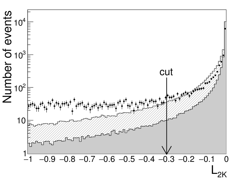
Figure 1: Distribution of $L_{\rm 2K}$ in data (points), simulation of $e^{+}e^{-}{\to}\phi\eta{\to}K^{+}K^{-}2\gamma$ (the grey histogram) and simulaion of $e^{+}e^{-}{\to}K^{+}K^{-}\eta{\to}K^{+}K^{-}2\gamma$ according to phase space (the dashed histogram). The simulated histograms are normalized to the number of events in the experimental one. Data at all energies are used.

\begin{overpic}[width=424.94574pt]{chi2_phase_space-eps-converted-to.pdf} \put(43.0,28.0){\includegraphics[width=216.81pt]{chi2_phieta-eps-converted-to.pdf}} \end{overpic}

Figure 2: Distribution of the $\chi^{2}_{\rm 4C}$ value in data (points) and simulation of $e^{+}e^{-}{\to}K^{+}K^{-}\eta{\to}K^{+}K^{-}2\gamma$ according to phase space (the dashed histogram), normalized to the $e^{+}e^{-}{\to}\phi\eta{\to}K^{+}K^{-}2\gamma$ cross section. The inset shows a similar distribution for the simulation of $e^{+}e^{-}{\to}\phi\eta{\to}K^{+}K^{-}2\gamma$ (the grey histogram). Data at all energies are used.

The resulting distributions of $dE/dx$ vs particle momentum, $m_{\rm inv,2\gamma}$ and $m_{\rm inv,2K}$ are shown in Figs. 4–6. It is seen that the $\phi\eta{\to}K^{+}K^{-}\eta$ mechanism dominates in the process. Furthermore, events with $m_{\rm inv,\,2K}>1075\,{\rm MeV}$ show no peaking structure near $m_{\rm inv,2\gamma}=m_{\eta}$, thus mainly coming from the background (the expected contribution of $\phi\eta{\to}K^{+}K^{-}2\gamma$ is about 30 events).

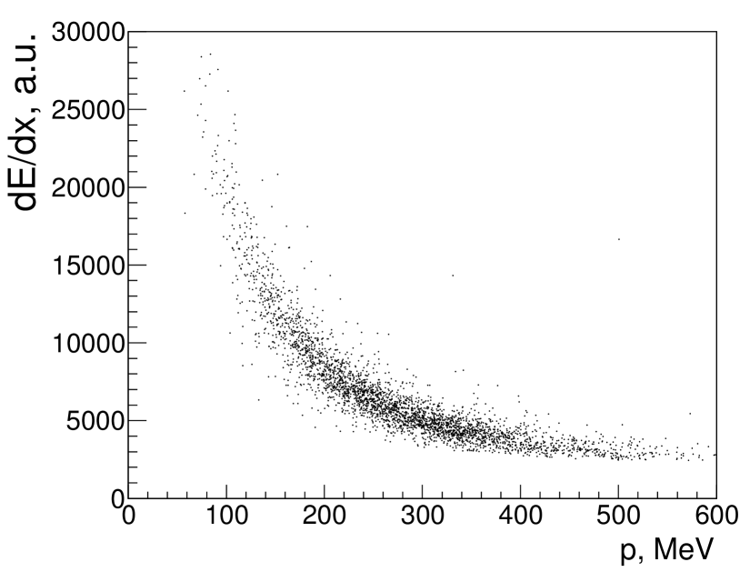
Figure 3: The distribution of $dE/dx$ vs particle momentum in data (all energies are used.)

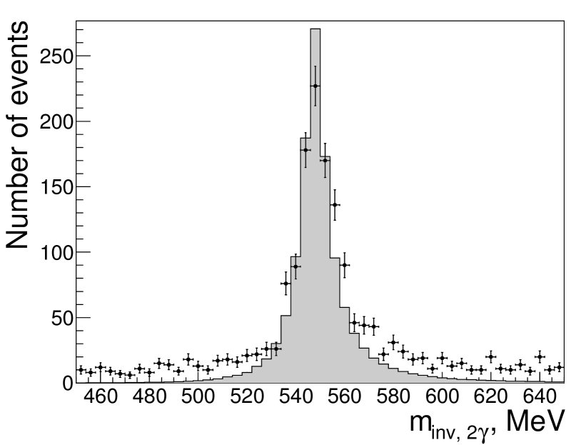
Figure 4: Distribution of $m_{\rm inv,2\gamma}$ in data (points) and simulation of $e^{+}e^{-}{\to}\phi\eta{\to}K^{+}K^{-}2\gamma$ (the grey histogram). Data at all energies are used.

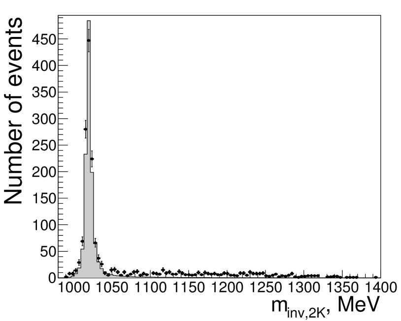
Figure 5: Distribution of $m_{\rm inv,2K}$ in data (points) and simulation of $e^{+}e^{-}{\to}\phi\eta{\to}K^{+}K^{-}2\gamma$ (the grey histogram). Data at all energies are used.

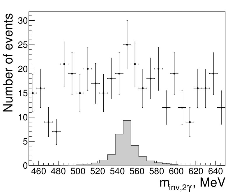
Figure 6: Distribution of the $m_{\rm inv,2\gamma}$ for events with $m_{\rm inv,2K}>1075\,\rm MeV$ in data (points) and simulation of $e^{+}e^{-}{\to}\phi\eta{\to}K^{+}K^{-}2\gamma$ (the grey histogram). Data at all energies are used.

Thus, we do not observe a contribution of any intermediate states in the process $e^{+}e^{-}{\to}K^{+}K^{-}\eta$ other than $\phi\eta$. In what follows we measure the cross section of the process $e^{+}e^{-}{\to}\phi\eta$ using the recoil to an $\eta$ meson. Such an inclusive approach allows us to avoid the loss of statistics due to selection of specific $\eta$ decay modes, but in turn it increases the amount of background.

3.2 Signal/background separation

We use the requirement $L_{\rm 2K}>-0.3$ to select events with two oppositely charged kaons and then the requirement $m_{\rm inv,\,2K}<1050\,{\rm MeV}$ to select events from the $\phi$-meson region, see Fig. 8. Simulation shows that the major background final states are $K^{+}K^{-}\pi^{0}\pi^{0}$ [22, 23] and $K^{+}K^{-}\pi^{+}\pi^{-}$ [23].

We perform the signal/background separation using the distribution of the ${\Delta}E$ parameter (Fig. 8), which is defined as

$${\Delta}E=\sqrt{\vec{p}^{2}_{K^{+}}+m^{2}_{K^{+}}}+\sqrt{\vec{p}^{2}_{K^{-}}+m^{2}_{K^{-}}}+\sqrt{(\vec{p}_{K^{+}}+\vec{p}_{K^{-}})^{2}+m^{2}_{\eta}}-E_{\rm c.m.},$$ (2)

and represents the “energy disbalance” of the event assuming the $\eta$ to be the recoil particle for the $K^{+}K^{-}$ pair.

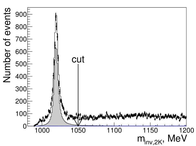
Figure 7: Distribution of the $m_{\rm inv,2K}$ in data (points), in simulation of the signal (the grey histogram) and of the signal and background processes (the open histogram). Data at all energies are used.

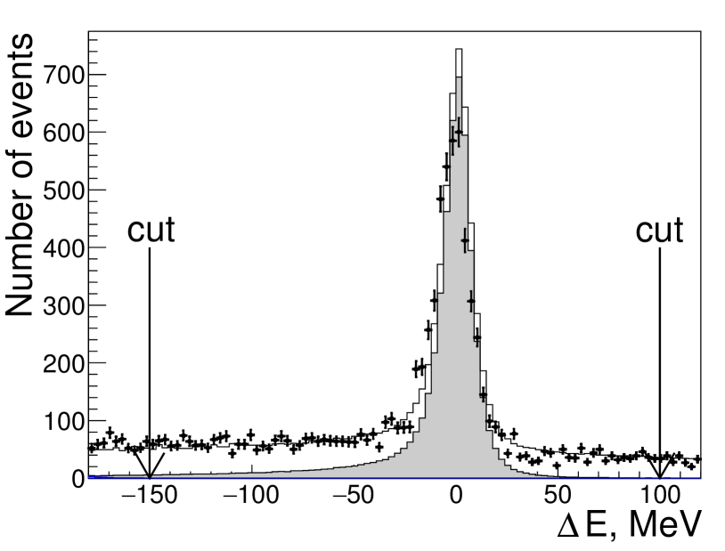
Figure 8: Distribution of ${\Delta}E$ in data (points), in simulation of the signal (the grey histogram) and of the signal and background processes (the open histogram). Data at all energies are used.

We approximate the distribution of ${\Delta}E$ in the range from –150 to 100 MeV at each $E_{\rm c.m.}$, see Fig. 10. The linear function is used to describe the background shape. The shape of the signal is determined at each $E_{\rm c.m.}$ by fitting the simulated signal ${\Delta}E$ distribution by the sum of three Gaussians:

$$f^{\rm MC}_{\rm sig}(x)=a_{0}\Bigl{(}a_{1}G(x,\mu_{1},\sigma_{1})+a_{2}G(x,\mu_{2},\sigma_{2})+(1-a_{1}-a_{2})G(x,\mu_{3},\sigma_{3})\Bigr{)},$$ (3)

$$G(x,\mu,\sigma)=\frac{1}{\sqrt{2\pi}\sigma}\exp\Biggl{(}-\frac{(x-\mu)^{2}}{2\sigma^{2}}\Biggr{)}.$$

In the fit of the experimental ${\Delta}E$ distribution we fix the parameters $a_{1,2}$, $\mu_{i}$ and $\sigma_{i}$ characterising the signal shape at the values obtained from the fit of the simulation. The signal amplitude $a_{0}$, the possible shift ${\delta}x$ and smearing $\delta\sigma$ of the signal distribution are taken as floating parameters:

$$f^{\rm exp}_{\rm sig}(x)=a_{0}\Bigl{(}a_{1}G(x,\mu_{1}+{\delta}x,\sqrt{\sigma^{2}_{1}+\delta\sigma^{2}})+a_{2}G(x,\mu_{2}+{\delta}x,\sqrt{\sigma^{2}_{2}+\delta\sigma^{2}})+$$ (4)

$$(1-a_{1}-a_{2})G(x,\mu_{3}+{\delta}x,\sqrt{\sigma^{2}_{3}+\delta\sigma^{2}})\Bigr{)}.$$

In total, 3009 $\pm$ 67 of signal events were selected.

3.3 Efficiencies

Figure 10 shows the detection efficiency for events of the signal process (including emission of photon jets by the initial electron and positron) according to simulation ($\varepsilon_{\rm MC}$) depending on $E_{\rm c.m.}$, calculated as the ratio of the number of detected events in simulation to the total number of simulated events. The nonmonotonous behaviour of $\varepsilon_{\rm MC}$ reflects the dependence of the geometrical detection efficiency of the kaon pair produced in the $\phi$-meson decay on the $\phi$-meson velocity. The “jumps” in $\varepsilon_{\rm MC}$ are related to the variation of the $dE/dx$ resolution at different energy points.

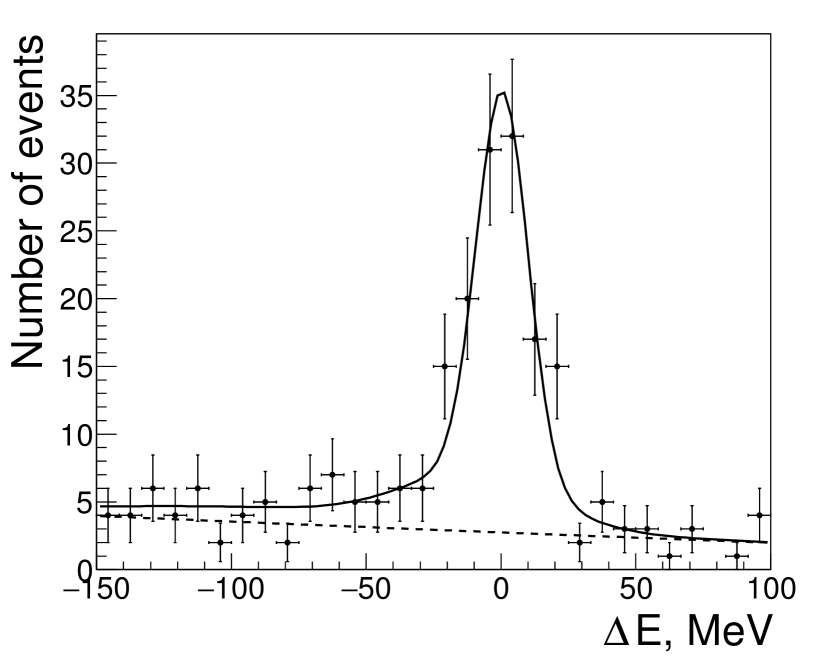
Figure 9: Signal/background separation at $E_{\rm c.m.}=1.967\,\rm GeV$ by a fit of the ${\Delta}E$ distribution in data (points). The solid line represents the fitting function, the dotted line - the part of this function related to the background.

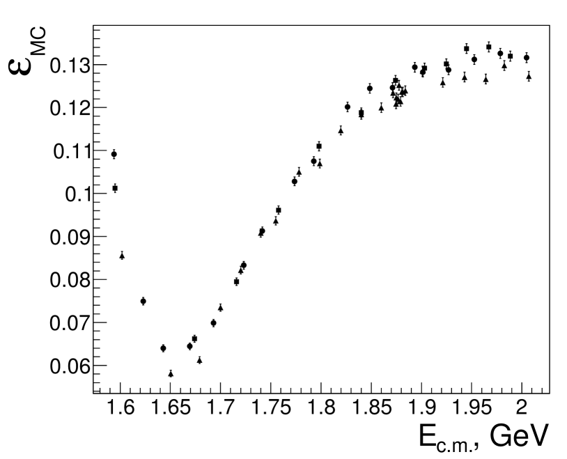
Figure 10: Detection efficiency for events of the process $e^{+}e^{-}{\to}K^{+}K^{-}\eta$ as a function of $E_{\rm c.m.}$.

In the study of the process $e^{+}e^{-}{\to}K^{+}K^{-}\pi^{+}\pi^{-}$ with the CMD-3 detector [22] it was found that the average detection efficiencies for kaons in experiment, ($\varepsilon^{K}_{\rm exp}$), and simulation, ($\varepsilon^{K}_{\rm MC}$), agree with the accuracy of 1% (the $0.85<\theta<\pi-0.85$ range was considered). Thus we estimate the systematic uncertainty of the kaon detection efficiency for the “good” polar angle range $1.0<\theta<\pi-1.0$ as less than $1\%$.

At polar angles $\theta<1.0$ and $\theta>\pi-1.0$ the kaon detection efficiency decreases in a different way in data and simulation, leading to the difference of the experimental and simulated kaon polar angle spectra. From that difference one can obtain the correction to the selection efficiency for the $K^{+}K^{-}\eta$ final state. To do this we select events from the signal peak region $-40\,{\rm MeV}<{\Delta}E<20\,{\rm MeV}$ with at least one kaon having the polar angle in the range 1.1 to $\pi-1.1$ (we assume $\varepsilon^{K}_{\rm exp}$ to be equal to $\varepsilon^{K}_{\rm MC}$ in this range). Figure 12 shows the comparison of the $|\pi/2-\theta|$ distributions for the second kaon in data and simulation. The approximation of the ratio of spectra in simulation and data by the function $1+\exp(p_{0}(p_{1}-\theta))$ provides a correction for the kaon selection efficiency $(1+\delta^{K}_{\rm eff})(\theta)$ as a function of $\theta$, see Fig. 12. The uncertainty of this function is obtained by the multifold variation of the points in the histogram, shown in Fig. 12, and it’s subsequent refitting.

The correction $(1+\delta_{\rm eff})$ for the kaons selection efficiency in $K^{+}K^{-}\eta$ final state is obtained as the convolution of $1/(1+\delta^{K}_{\rm eff})(\theta)$ with the polar angle distributions of the kaons reconstructed in simulation:

$$(1+\delta_{\rm eff})=\frac{1}{N_{\rm sim.rec.}}\sum^{i=N_{\rm sim.rec.}}_{i=1}\frac{1}{(1+\delta^{K}_{\rm eff}(\theta_{K^{-}}))\cdot(1+\delta^{K}_{\rm eff}(\theta_{K^{+}}))}.$$ (5)

The values of this correction at different energies are shown in Fig. 14. The systematic uncertainty of these values is derived from the uncertainty of $(1+\delta^{K}_{\rm eff})(\theta)$ function and is estimated to be 1.5%. To test the validity of the obtained correction, we use the value of the estimated total number of signal events $N_{\rm sig.tot}$, actually produced at the collider during the experimental runs:

$$N_{\rm sig.tot}=\sum_{i=1}^{N_{\rm en.points}}\frac{N^{i}_{\rm sig.events}}{\varepsilon^{i}},$$ (6)

where $N^{i}_{\rm sig.events}$ is the number of selected signal events at the $i$-th energy, $\varepsilon^{i}$ – the corrected detection efficiency at that energy. Application of the efficiency correction makes $N_{\rm sig.tot}$ almost independent of $\theta_{\rm cut}$, as one can see from Fig. 14.

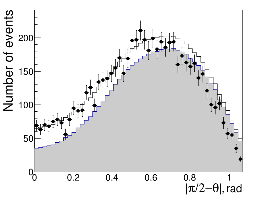
Figure 11: Distribution of $|\pi/2-\theta|$ for the second kaon in the experiment and in the simulation of the signal (the grey histogram) and of the signal and background processes (the open histogram). The histogram for the simulation of signal and background is normalized in the range $|\pi/2-\theta|<0.5$ to the experimental one in the same range.

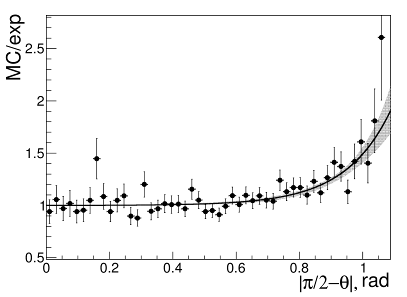
Figure 12: Approximation of the ratio of the $|\pi/2-\theta|$ distribution for the second kaon in the simulation of the signal and background processes to that in the experiment. The shaded area shows the uncertainty of the fitting function.

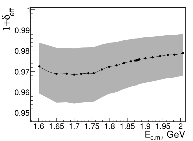
Figure 13: Correction $(1+\delta_{\rm eff})$ to the detection efficiency of events of the process $e^{+}e^{-}{\to}K^{+}K^{-}\eta$ as a function of $E_{\rm c.m.}$ for the runs of 2017. The shaded area shows the uncertainty of the correction.

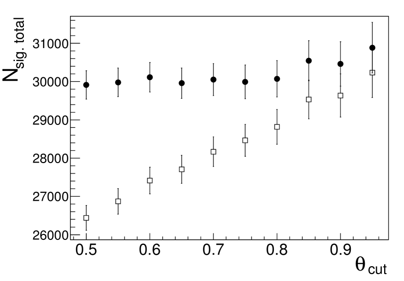
Figure 14: Dependence of $N_{\rm sig.tot}$ on $\theta_{\rm cut}$ before (open bars) and after (filled circles) application of the efficiency correction.

Next, since the $\varepsilon_{\rm MC}$ value does not include the trigger efficiency $\varepsilon_{\rm trig}$, the latter should be found separately from the experimental data. The trigger of the CMD-3 detector consists of two subsystems, so-called “neutral” trigger (NT) and “charged” trigger (CT), connected into the OR scheme, and the overall trigger efficiency equals

$$\varepsilon_{\rm trig}=1-(1-\varepsilon_{\rm NT})(1-\varepsilon_{\rm CT}),$$ (7)

where the efficiencies of NT and CT are expressed in terms of the number of events in the experiment, in which only NT ($N_{\rm NT}$), only CT ($N_{\rm CT}$) or both subsystems ($N_{\rm NT{\&}CT}$) were triggered:

$$\varepsilon_{\rm NT}=\frac{N_{\rm NT\&CT}}{N_{\rm NT\&CT}+N_{\rm CT}},\,\varepsilon_{\rm CT}=\frac{N_{\rm NT\&CT}}{N_{\rm NT\&CT}+N_{\rm NT}}.$$ (8)

Figure 16 shows the values of $\varepsilon_{\rm trig}$, $\varepsilon_{\rm NT}$ and $\varepsilon_{\rm CT}$ as the functions of $E_{\rm c.m.}$ for the runs of 2012. Finally, the corrected detection efficiency $\varepsilon$ is calculated as

$$\varepsilon=\varepsilon_{\rm MC}(1+\delta_{\rm eff})\varepsilon_{\rm trig}.$$ (9)

3.4 Cross section calculation and approximation

The Born cross section of the process $e^{+}e^{-}{\to}\phi\eta$ at each $E_{\rm c.m.}$ is calculated by dividing the visible cross section $\sigma_{\rm vis}$ by the radiative correction $(1+\delta_{\rm rad})$:

$$\sigma_{\rm Born}=\frac{\sigma_{\rm vis}}{1+\delta_{\rm rad}}=\frac{N_{\rm sig.events}}{L\varepsilon(1+\delta_{\rm rad})\mathcal{B}^{\phi}_{K^{+}K^{-}}},$$ (10)

where $N_{\rm sig.events}$ is the number of selected events of the signal process, $L$ – the integrated luminosity, $\varepsilon$ – the corrected detection efficiency. To calculate the radiative correction at each $E_{\rm c.m.}$ point we use the $F(x,E_{\rm c.m.})$ structure function [24]:

$$1+\delta_{\rm rad}=\int\limits_{0}^{1}dx\,F(x,E_{\rm c.m.})\frac{\sigma_{\rm Born}(E_{\rm c.m.}\sqrt{1-x})}{\sigma_{\rm Born}(E_{\rm c.m.})}.$$ (11)

We perform the calculation iteratively, using for the first iteration the approximation of the cross section measured by BaBar [6], in the $E_{\rm c.m.}$ range from 1.58 to 2.0 and from 2.3 to 3.5 GeV (excluding the region from 2.0 to 2.3 GeV to avoid the fitting of the $\phi(2170)$ resonance). For the cross section approximation we use the formula

$$\sigma_{\phi\eta}(s)=\frac{27\Gamma_{\phi}m^{2}_{\phi}}{\pi^{2}|\vec{p}_{K}(m_{\phi})|^{3}s}F(s){\Biggl{|}}\frac{a_{\rm n.r.}e^{i\Psi_{\rm n.r.}}}{s}+\sqrt{\frac{(\Gamma^{\phi^{\prime}}_{ee}\mathcal{B}^{\phi^{\prime}}_{\phi\eta})\Gamma_{\phi^{\prime}}m^{3}_{\phi^{\prime}}}{|\vec{p}_{\phi}(m_{\phi^{\prime}})|^{3}}}D_{\phi^{\prime}}(s){\Biggr{|}}^{2},$$ (12)

$$F(s)={\int}|\vec{p}_{K^{+}}{\times}\vec{p}_{K^{-}}|^{2}\sin^{2}(\theta_{\rm normal})|D_{\phi}(p^{2}_{\phi})|^{2}d\Phi_{K^{+}K^{-}\eta}(\sqrt{s}),$$ (13)

where $D_{\phi^{\prime}}(s)=1/(s-m^{2}_{\phi^{\prime}}+i\sqrt{s}\Gamma_{\phi^{\prime}}(s))$ and $D_{\phi}(p^{2}_{\phi})=1/(p^{2}_{\phi}-m^{2}_{\phi}+i\sqrt{p^{2}_{\phi}}\Gamma_{\phi}(p^{2}_{\phi}))$ are the $\phi^{\prime}$ and $\phi$ propagators, $|\vec{p}_{\phi}(\sqrt{s})|$ is the momentum of the $\phi$ in the $\phi^{\prime}{\to}\phi\eta$ decay in the $\phi^{\prime}$ rest frame, $|\vec{p}_{K}(\sqrt{p^{2}_{\phi}})|$ is the momentum of the kaon in the $\phi{\to}K^{+}K^{-}$ decay in the $\phi$ rest frame, $\theta_{\rm normal}$ is the polar angle of the normal to the plane formed by the $\vec{p}_{K^{+}}$ and $\vec{p}_{K^{-}}$ vectors, $d\Phi_{K^{+}K^{-}\eta}$ is the element of three-body phase space. We neglect the OZI-suppressed [25] contribution of $\omega(1650)$, but consider the possible contributiuon of the resonance below reaction threshold, describing it via the amplitude $a_{\rm n.r.}e^{i\Psi_{\rm n.r.}}/s$. The factor $F(s)$ represents the “dynamic” part of the squared matrix element averaged over the three-body $K^{+}K^{-}\eta$ phase space.

The quantity $\Gamma_{\phi^{\prime}}(s)$ is given by the following expression (see [23]):

$$\Gamma_{\phi^{\prime}}(s)=\Gamma_{\phi^{\prime}}\Biggl{[}\mathcal{B}^{\phi^{\prime}}_{K^{*}(892)K}\frac{\mathcal{P}_{K^{*}(892)K}(s)}{\mathcal{P}_{K^{*}(892)K}(m_{\phi^{\prime}}^{2})}+\mathcal{B}^{\phi^{\prime}}_{\phi\eta}\frac{\mathcal{P}_{\phi\eta}(s)}{\mathcal{P}_{\phi\eta}(m_{\phi^{\prime}}^{2})}+\mathcal{B}^{\phi^{\prime}}_{\phi\sigma}\frac{\mathcal{P}_{\phi\sigma}(s)}{\mathcal{P}_{\phi\sigma}(m_{\phi^{\prime}}^{2})}\Biggr{]},$$ (14)

where $\sigma$ designates the $f_{0}(500)$ meson, the $\mathcal{P}_{K^{*}(892)K}$ and $\mathcal{P}_{\phi\eta}$ functions represent the phase spaces of quasi-two-body final states in $\phi^{\prime}{\to}K^{*}(892)K$ and $\phi^{\prime}{\to}\phi\eta$ decays. According to [23] we take $\mathcal{B}^{\phi^{\prime}}_{K^{*}(892)K}=0.7$, $\mathcal{B}^{\phi^{\prime}}_{\phi\eta}=0.2$, $\mathcal{B}^{\phi^{\prime}}_{\phi\sigma}=0.1$. The $K^{*}K$ and $\phi\eta$ phase space factors have the form:

$$\mathcal{P}_{VP}(s)=\Biggl{[}\frac{(s+m^{2}_{V}-m^{2}_{P})^{2}-4m^{2}_{V}s}{s}\Biggl{]}^{\frac{3}{2}},$$ (15)

where $V=K^{*},\phi$, $P=K,\eta$. The $\mathcal{P}_{{\phi}\sigma}$ function in (14) represents the phase space of the quasi-two-body final state in $\phi^{\prime}{\to}{\phi}\sigma$ decay and is calculated as:

$$\mathcal{P}_{{\phi}\sigma}(s)={\int^{\sqrt{s}-m_{\phi}}_{2m_{\pi}}}dm|BW(m,m_{\sigma},\Gamma_{\sigma})|^{2}(\mathcal{P}_{{\phi}\sigma})|_{m_{\sigma}=m},$$ (16)

where

$$|BW(m,m_{\sigma},\Gamma_{\sigma})|^{2}=\frac{2m_{\sigma}\Gamma_{\sigma}m}{{\pi}((m^{2}-m_{\sigma}^{2})^{2}+m_{\sigma}^{2}\Gamma_{\sigma}^{2})}$$ (17)

is the probability density for $\sigma$ to have a mass $m$, which can be approximately estimated as a squared module of the Breit-Wigner function $BW(m,m_{\sigma},\Gamma_{\sigma})$ with the $m_{\sigma}$ central value and the $\Gamma_{\sigma}$ width (we set $m_{\sigma}=0.475\,\rm GeV$ and $\Gamma_{\sigma}=0.550\,\rm GeV$ [26]), and

$$(\mathcal{P}_{{\phi}\sigma})|_{m_{\sigma}=m}=\frac{\sqrt{(s+m^{2}_{\phi}-m^{2})^{2}-4sm^{2}_{\phi}}}{s^{3/2}}{\Biggl{(}}1+\frac{(s+m_{\phi}^{2}-m^{2})^{2}}{8sm_{\phi}^{2}}{\Biggr{)}}$$ (18)

is the quantity proportional to the width of the $\phi^{\prime}{\to}{\phi}\sigma$ decay with the $\sigma$ mass equal to $m$. Integration in the formula 16 is performed in the range available for $m=m_{\rm inv,2\pi}\in(2m_{\pi};\sqrt{s}-m_{\phi})$.

Similarly to $\Gamma_{\phi^{\prime}}(s)$ the $\Gamma_{\phi}(s)$ is calculated taking into account the $K^{+}K^{-}$, $K_{S}K_{L}$ and $\pi^{+}\pi^{-}\pi^{0}$ modes of $\phi$-meson decay.

It should be noted that in the work of BaBar [6] for the $e^{+}e^{-}{\to}\phi\eta$ cross section fit the quasi-two-body formula

$$\sigma_{\phi\eta}(s)=12\pi\frac{|\vec{p}_{\phi}(\sqrt{s})|^{3}}{s^{3/2}}{\Biggl{|}}\frac{a_{\rm n.r.}e^{i\Psi_{\rm n.r.}}}{s}+\sqrt{\frac{(\Gamma^{\phi^{\prime}}_{ee}\mathcal{B}^{\phi^{\prime}}_{\phi\eta})\Gamma_{\phi^{\prime}}m^{3}_{\phi^{\prime}}}{|\vec{p}_{\phi}(m_{\phi^{\prime}})|^{3}}}D_{\phi^{\prime}}(s){\Biggr{|}}^{2}$$ (19)

was used. The normalized difference $(\sigma^{\rm 3body}_{\phi\eta}/\sigma^{\rm 2body}_{\phi\eta}-1)$ of the three-body and quasi-two-body cross section parametrizations is shown in Fig. 16. At the current level of a systematic uncertainty (see Section 3.5) it becomes important for us to use a more precise three-body formula.

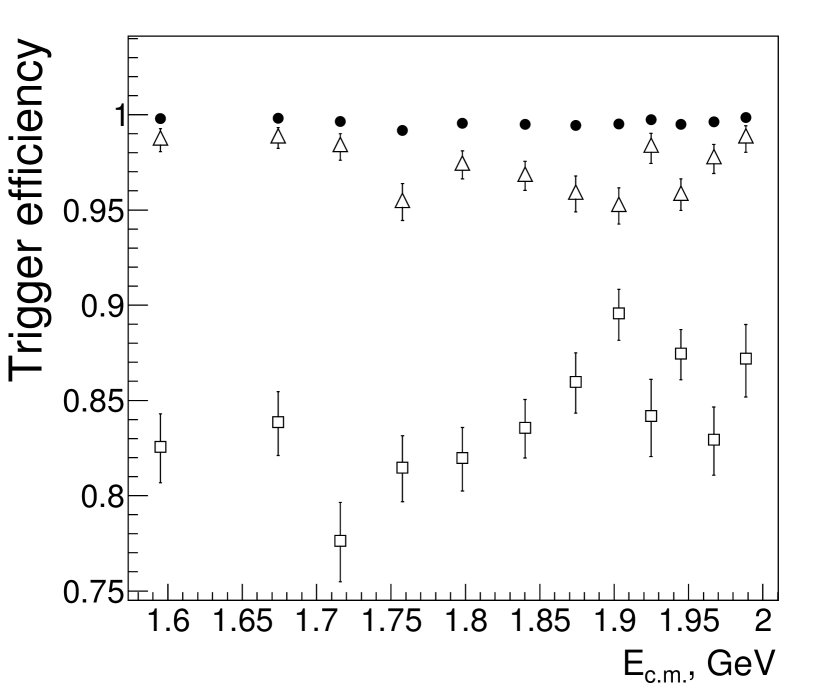
Figure 15: The $\varepsilon_{\rm trig}$ (circles), $\varepsilon_{\rm NT}$ (open bars) and $\varepsilon_{\rm CT}$ (open triangles) values as the functions of $E_{\rm c.m.}$ for the runs of 2012.

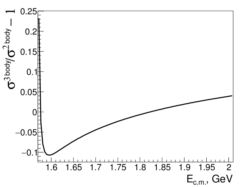
Figure 16: Normalized difference $(\sigma^{\rm 3body}_{\phi\eta}/\sigma^{\rm 2body}_{\phi\eta}-1)$ of the two cross section parametrizations.

After the first iteration we use CMD-3 data along with the BaBar data in the range from 2.3 to 3.5 GeV, which is necessary to fix the asymptotic behavior of the cross section. Four iterations are sufficient for the radiative corrections to converge with the accuracy of 0.5%. Figure 18 shows the values of the radiative correction at the last iteration. The uncertainties of the radiative corrections caused by the cross section shape are calculated by the multifold variation of the visible cross sections and subsequent recalculation of the radiative corrections and were found to be $<1.5\%$.

The obtained $e^{+}e^{-}{\to}\phi\eta$ Born cross section (see Tables 1–3) along with that of BaBar [6] and SND [8] is shown in Fig. 18. The fit of the cross section asymptotics is shown in Fig. 20. The obtained Born cross section exhibits a hint to the wavelike deviation from the fit near $E_{\rm c.m.}{\approx}1.9{\,}\rm GeV$, see Fig. 20. This may be due to the uncertainties of the branching fractions of $\phi^{\prime}$ decay modes or due to the decay modes, that were not taken into account in our cross section parameterization. Hovewer, at the current level of statistics we are not sensitive to these effects.

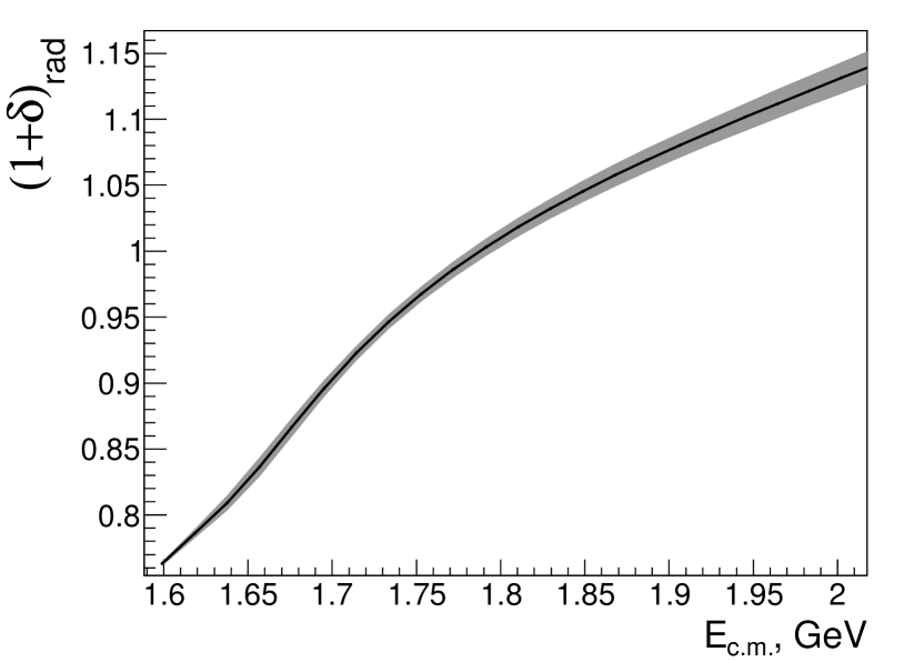
Figure 17: The radiative correction depending on $E_{\rm c.m.}$ at the last iteration (the solid curve) and its uncertainty (the shaded area).

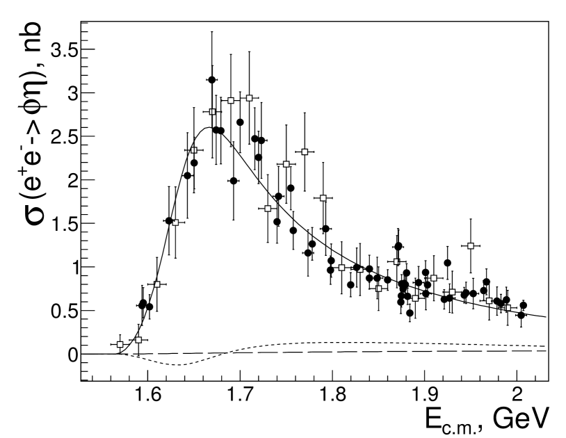
Figure 18: BaBar (open bars), SND (open triangles) and CMD-3 (filled circles) results for the measurement of the $e^{+}e^{-}{\to}\phi\eta$ cross section. The overall fit of CMD-3 data (the solid curve), nonresonant part (the dashed curve) and the interference part of the fit (the dotted curve) are shown.

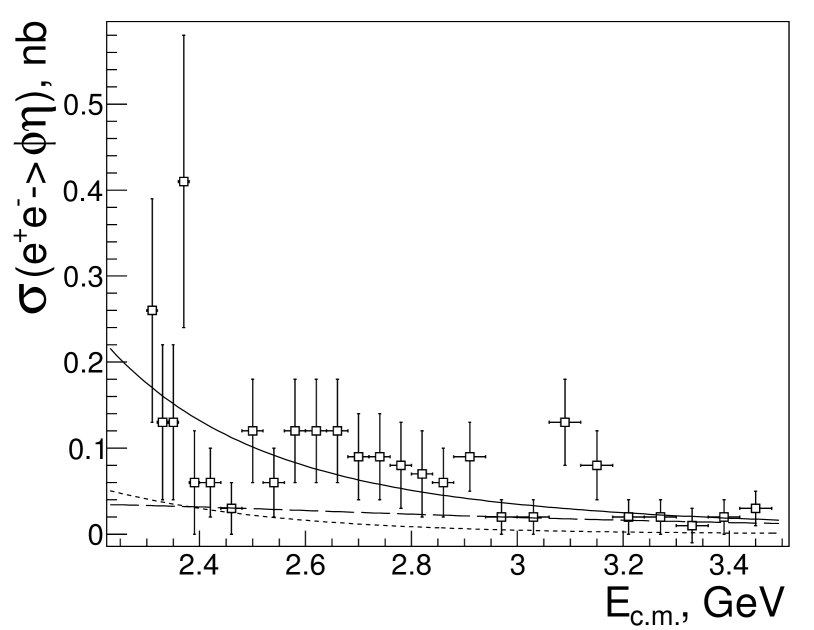
Figure 19: Approximation of the $e^{+}e^{-}{\to}\phi\eta$ process cross section measured by BaBar (open bars) in the $E_{\rm c.m.}$ range from 2.3 to 3.5 GeV (last iteration). The overall fit (the solid curve), nonresonant part (the dashed curve) and the interference part of the fit (the dotted curve) are shown.

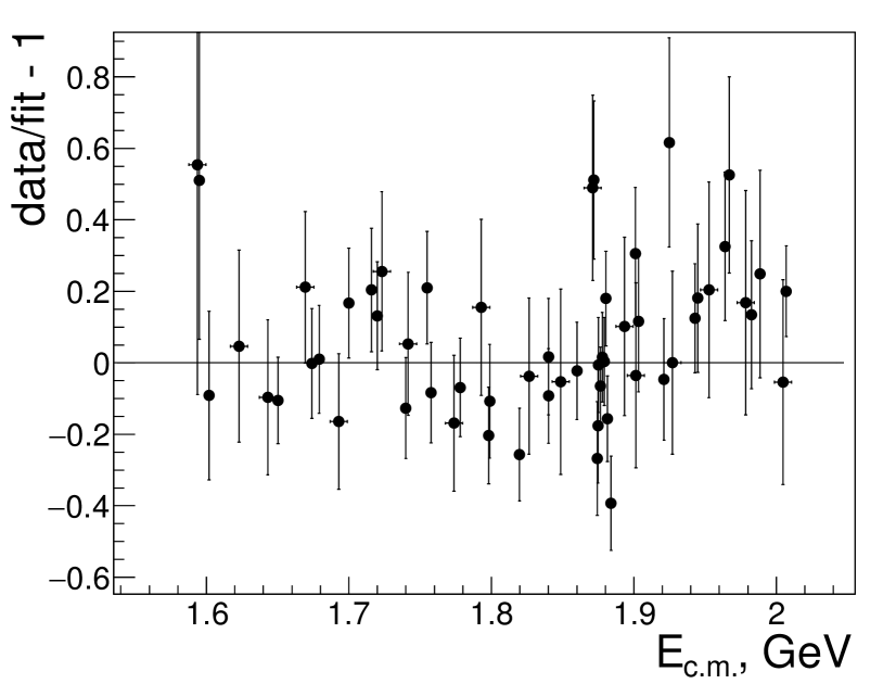
Figure 20: Normalized difference between the $e^{+}e^{-}{\to}\phi\eta$ cross section measured by CMD-3 and its approximation.

Table 1: Center-of-mass energy $E_{\rm c.m.}$, integrated luminosity $L$, number of signal events $N_{\rm sig.events}$, corrected detection efficiency $\varepsilon$, radiative correction $(1+\delta_{\rm rad})$ and Born cross section of $e^{+}e^{-}{\to}\phi\eta$ for the runs of 2011. The uncertainty of $E_{\rm c.m.}$ determination is 6 MeV. Only statistical uncertainties are shown.

$E_{\rm c.m.},\rm\,GeV$	$L$, nb-1	$N_{\rm sig.events}$	$\varepsilon$	$1+\delta_{\rm rad}$	$\sigma$, nb
1.594	450.0	6.8 $\pm$ 2.7	0.073 $\pm$ 0.006	0.76	0.56 $\pm$ 0.23
1.623	518.9	18.4 $\pm$ 4.7	0.060 $\pm$ 0.002	0.79	1.53 $\pm$ 0.39
1.643	463.3	21.3 $\pm$ 5.1	0.056 $\pm$ 0.001	0.82	2.05 $\pm$ 0.49
1.669	573.2	41.6 $\pm$ 7.2	0.055 $\pm$ 0.001	0.86	3.15 $\pm$ 0.55
1.693	494.7	27.0 $\pm$ 6.1	0.063 $\pm$ 0.001	0.89	1.99 $\pm$ 0.45
1.723	531.7	44.2 $\pm$ 7.8	0.074 $\pm$ 0.001	0.93	2.45 $\pm$ 0.44
1.742	542.5	39.0 $\pm$ 7.4	0.085 $\pm$ 0.001	0.95	1.81 $\pm$ 0.34
1.774	561.6	29.9 $\pm$ 6.8	0.095 $\pm$ 0.001	0.98	1.16 $\pm$ 0.27
1.793	455.4	32.5 $\pm$ 6.9	0.102 $\pm$ 0.001	1.00	1.44 $\pm$ 0.31
1.826	514.9	29.1 $\pm$ 6.6	0.113 $\pm$ 0.001	1.02	0.99 $\pm$ 0.23
1.849	436.0	22.5 $\pm$ 6.2	0.117 $\pm$ 0.001	1.04	0.87 $\pm$ 0.24
1.871	672.8	50.2 $\pm$ 8.7	0.118 $\pm$ 0.001	1.05	1.23 $\pm$ 0.21
1.893	528.7	28.2 $\pm$ 6.4	0.125 $\pm$ 0.001	1.06	0.82 $\pm$ 0.19
1.901	506.5	23.4 $\pm$ 6.3	0.128 $\pm$ 0.001	1.07	0.69 $\pm$ 0.19
1.927	566.8	24.3 $\pm$ 6.2	0.126 $\pm$ 0.001	1.08	0.64 $\pm$ 0.16
1.953	452.0	21.8 $\pm$ 5.5	0.130 $\pm$ 0.001	1.09	0.69 $\pm$ 0.17
1.978	522.5	22.1 $\pm$ 5.9	0.129 $\pm$ 0.001	1.11	0.61 $\pm$ 0.16
2.005	481.3	15.3 $\pm$ 4.6	0.131 $\pm$ 0.001	1.12	0.44 $\pm$ 0.13

Table 2: Center-of-mass energy $E_{\rm c.m.}$, integrated luminosity $L$, number of signal events $N_{\rm sig.events}$, corrected detection efficiency $\varepsilon$, radiative correction $(1+\delta_{\rm rad})$ and Born cross section of $e^{+}e^{-}{\to}\phi\eta$ for the runs of 2012. The uncertainty of $E_{\rm c.m.}$ determination is 2 MeV. Only statistical uncertainties are shown.

$E_{\rm c.m.},\rm\,GeV$	$L$, nb-1	$N_{\rm sig.events}$	$\varepsilon$	$1+\delta_{\rm rad}$	$\sigma$, nb
1.595	835.068	14.4 $\pm$ 4.1	0.076 $\pm$ 0.002	0.76	0.62 $\pm$ 0.18
1.674	896.135	57.1 $\pm$ 8.8	0.059 $\pm$ 0.001	0.87	2.57 $\pm$ 0.40
1.716	815.996	66.5 $\pm$ 9.5	0.073 $\pm$ 0.001	0.92	2.47 $\pm$ 0.35
1.758	972.844	60.2 $\pm$ 9.2	0.092 $\pm$ 0.001	0.97	1.42 $\pm$ 0.22
1.798	999.604	48.8 $\pm$ 8.3	0.103 $\pm$ 0.001	1.00	0.96 $\pm$ 0.16
1.840	967.496	55.3 $\pm$ 8.9	0.116 $\pm$ 0.001	1.03	0.98 $\pm$ 0.16
1.874	857.024	32.7 $\pm$ 7.1	0.124 $\pm$ 0.001	1.05	0.60 $\pm$ 0.13
1.903	901.701	47.6 $\pm$ 8.4	0.127 $\pm$ 0.001	1.07	0.79 $\pm$ 0.14
1.925	567.388	41.2 $\pm$ 7.4	0.131 $\pm$ 0.001	1.08	1.05 $\pm$ 0.19
1.945	995.035	47.3 $\pm$ 8.3	0.127 $\pm$ 0.001	1.09	0.70 $\pm$ 0.12
1.967	693.468	41.0 $\pm$ 7.4	0.132 $\pm$ 0.001	1.10	0.83 $\pm$ 0.15
1.988	601.598	26.9 $\pm$ 6.2	0.132 $\pm$ 0.001	1.11	0.62 $\pm$ 0.14

Table 3: Center-of-mass energy $E_{\rm c.m.}$, integrated luminosity $L$, number of signal events $N_{\rm sig.events}$, corrected detection efficiency $\varepsilon$, radiative correction $(1+\delta_{\rm rad})$ and Born cross section of $e^{+}e^{-}{\to}\phi\eta$ for the runs of 2017. The uncertainty of $E_{\rm c.m.}$ determination is 50 keV. Only statistical uncertainties are shown.

$E_{\rm c.m.},\rm\,GeV$	$L$, nb-1	$N_{\rm sig.events}$	$\varepsilon$	$1+\delta_{\rm rad}$	$\sigma$, nb
1.602	1275.5	18.3 $\pm$ 4.7	0.071 $\pm$ 0.001	0.77	0.54 $\pm$ 0.14
1.650	1428.8	65.6 $\pm$ 8.8	0.052 $\pm$ 0.001	0.83	2.19 $\pm$ 0.30
1.679	1009.5	60.1 $\pm$ 8.9	0.054 $\pm$ 0.001	0.87	2.56 $\pm$ 0.38
1.700	947.0	73.0 $\pm$ 9.5	0.066 $\pm$ 0.001	0.90	2.66 $\pm$ 0.35
1.720	923.6	71.7 $\pm$ 9.5	0.076 $\pm$ 0.001	0.93	2.26 $\pm$ 0.30
1.740	947.4	55.8 $\pm$ 9.0	0.083 $\pm$ 0.001	0.95	1.52 $\pm$ 0.25
1.755	1048.4	82.9 $\pm$ 10.8	0.088 $\pm$ 0.001	0.97	1.90 $\pm$ 0.25
1.778	1139.7	67.2 $\pm$ 9.9	0.097 $\pm$ 0.001	0.99	1.26 $\pm$ 0.19
1.799	880.9	48.0 $\pm$ 8.6	0.103 $\pm$ 0.001	1.00	1.07 $\pm$ 0.19
1.820	1161.7	50.2 $\pm$ 8.7	0.109 $\pm$ 0.001	1.02	0.79 $\pm$ 0.14
1.840	1378.3	68.6 $\pm$ 10.0	0.113 $\pm$ 0.001	1.03	0.87 $\pm$ 0.13
1.860	1550.5	78.9 $\pm$ 11.0	0.117 $\pm$ 0.001	1.05	0.85 $\pm$ 0.12
1.872	1055.5	80.5 $\pm$ 11.7	0.119 $\pm$ 0.001	1.05	1.24 $\pm$ 0.18
1.875	1088.3	44.6 $\pm$ 8.6	0.119 $\pm$ 0.001	1.05	0.67 $\pm$ 0.13
1.875	1900.0	94.0 $\pm$ 12.6	0.119 $\pm$ 0.001	1.05	0.80 $\pm$ 0.11
1.877	2538.6	117.1 $\pm$ 13.5	0.119 $\pm$ 0.001	1.05	0.75 $\pm$ 0.09
1.878	2063.5	103.8 $\pm$ 12.7	0.120 $\pm$ 0.001	1.06	0.81 $\pm$ 0.10
1.879	2024.8	99.3 $\pm$ 12.2	0.119 $\pm$ 0.001	1.06	0.80 $\pm$ 0.10
1.880	1907.2	110.7 $\pm$ 12.4	0.121 $\pm$ 0.001	1.06	0.93 $\pm$ 0.10
1.881	1874.3	78.7 $\pm$ 11.2	0.122 $\pm$ 0.001	1.06	0.66 $\pm$ 0.09
1.884	1341.7	39.5 $\pm$ 8.6	0.121 $\pm$ 0.001	1.06	0.47 $\pm$ 0.10
1.901	1179.9	71.5 $\pm$ 10.1	0.124 $\pm$ 0.001	1.07	0.94 $\pm$ 0.13
1.921	1354.4	55.6 $\pm$ 9.9	0.124 $\pm$ 0.001	1.08	0.63 $\pm$ 0.11
1.943	1787.7	78.8 $\pm$ 10.7	0.123 $\pm$ 0.001	1.09	0.68 $\pm$ 0.09
1.964	1326.1	65.0 $\pm$ 10.2	0.125 $\pm$ 0.001	1.10	0.73 $\pm$ 0.11
1.983	1254.5	49.5 $\pm$ 9.0	0.126 $\pm$ 0.001	1.11	0.58 $\pm$ 0.11
2.007	3809.4	143.5 $\pm$ 15.1	0.123 $\pm$ 0.001	1.12	0.56 $\pm$ 0.06

The $\phi^{\prime}$ parameters, obtained from the approximation of the CMD-3 cross section are shown in Table 4. Along with the cross section parametrization using $\Gamma^{\phi^{\prime}}_{ee}\mathcal{B}^{\phi^{\prime}}_{\phi\eta}$ we also tried the parametrization through $\mathcal{B}^{\phi^{\prime}}_{e^{+}e^{-}}\mathcal{B}^{\phi^{\prime}}_{\phi\eta}$. The results for all other fit parameters but $\Gamma^{\phi^{\prime}}_{ee}\mathcal{B}^{\phi^{\prime}}_{\phi\eta}$ and $\mathcal{B}^{\phi^{\prime}}_{e^{+}e^{-}}\mathcal{B}^{\phi^{\prime}}_{\phi\eta}$ are the same in both cases. Our results for $\phi^{\prime}$ parameters are compatible with those of BaBar [6] and other previous measurements, but have better statistical precision. The estimation of the systematic uncertainties of $\phi^{\prime}$ parameters is described in Section 3.5.

Table 4: Results of the $e^{+}e^{-}{\to}\phi\eta$ cross section approximation.

Parametrization using	$\Gamma^{\phi^{\prime}}_{ee}\mathcal{B}^{\phi^{\prime}}_{\phi\eta}$	$\mathcal{B}^{\phi^{\prime}}_{e^{+}e^{-}}\mathcal{B}^{\phi^{\prime}}_{\phi\eta}$
Parameter	Value
$\chi^{2}/{\rm n.d.f}$	$93.8/79{\approx}1.19$
$\Gamma^{\phi^{\prime}}_{ee}\mathcal{B}^{\phi^{\prime}}_{\phi\eta},\rm eV$	$94{\pm}13_{\rm stat}{\pm}15_{\rm syst}$	–
$\mathcal{B}^{\phi^{\prime}}_{e^{+}e^{-}}\mathcal{B}^{\phi^{\prime}}_{\phi\eta}$	–	$0.53{\pm}0.06_{\rm stat}{\pm}0.09_{\rm syst}$
$m_{\phi^{\prime}},\rm MeV$	$1667{\pm}5_{\rm stat}{\pm}11_{\rm syst}$
$\Gamma_{\phi^{\prime}},\rm MeV$	$176{\pm}23_{\rm stat}{\pm}38_{\rm syst}$
$a_{\rm n.r.},\rm MeV$	$1.1{\pm}0.6_{\rm stat}$
$\Psi_{\rm n.r.}$	$0.14{\pm}0.67_{\rm stat}$

3.5 Systematic uncertainties

We estimate a systematic uncertainty related to some selection criterion as a relative variation of the $N_{\rm sig.tot}$ (see Section 3.3) with the variation (or swithcing on/off) of this criterion. The limits for the variation of the cuts are chosen as wide as possible with two requirements: 1) restriction does not seriously cut the signal; 2) the background shape is reasonably described by the contribution of $K^{+}K^{-}\pi^{0}\pi^{0}$ and $K^{+}K^{-}\pi^{+}\pi^{-}$ final states. The following sources of systematic uncertainties were considered:

• The requirements on $\rho_{\rm PCA}$, $z_{\rm PCA}$, $p_{\perp}$ and $dE/dx<(dE/dx)_{\rm protons}$ for positively charged particles applied in the “good” track selection procedure, give the uncertainties of 1.0, 0.5, 0.3 and 0.4$\%$, respectively. The values are estimated by swithcing on/off these requirements.

• The cut on $L_{\rm 2K}$ used for the kaon selection was varied from -0.6 to -0.1. The corresponding uncertainty was 0.8$\%$.

• The cut on $m_{\rm inv,2K}$, used for the $\phi$-meson region selection, was varied from 1050 to 1100 MeV. The corresponding uncertainty was 0.7$\%$.

• The lower limit of the ${\Delta}E$ distribution fit was varied from $-180$ to $-100$ MeV. The corresponding uncertainty was 1$\%$.

• The upper limit of the ${\Delta}E$ distribution fit was varied from $50$ to $150$ MeV. The corresponding uncertainty was 1$\%$.

• The signal peak position can be fixed from simulation ($\delta x\equiv 0$) or released in the fit of the experimental $\Delta E$ distribution, the corresponding uncertainty is 2$\%$.

• The signal width can be fixed from the simulation ($\delta\sigma\equiv 0$) or released, the corresponding uncertainty is 2.5$\%$.

• The background shape in the fit of the experimental $\Delta E$ distribution can be taken as linear with floating parameters, or it can be fixed from the fit of the simulated background distribution. The corresponding uncertainty is 2.3$\%$.

• The uncertainty of the single kaon detection efficiency is estimated to be 1$\%$, for the pair of kaons – 1.5$\%$. The uncertainty of the correction to the $K^{+}K^{-}\eta$ selection efficiency related to the angular dependence of the kaon detection efficiency (see Section 3.3), was estimated to be 1.5$\%$.

• The systematic uncertainty of the luminosity measurement is 1$\%$ [18].

• The uncertainty of the $\mathcal{B}^{\phi}_{K^{+}K^{-}}$ is about 1$\%$.

Table 5 shows a summary of the analyzed systematic uncertainties of the cross section measurement. The overall systematic uncertainty is obtained by a quadratic summation of the individual uncertainties and is estimated to be 5.1$\%$.

The following contributions to the systematic uncertainties of the $\phi^{\prime}$ parameters were analyzed:

• The systematic uncertainty of cross section measurement induces 5.1% uncertainty of $\Gamma^{\phi^{\prime}}_{ee}\mathcal{B}^{\phi^{\prime}}_{\phi\eta}$ and $\mathcal{B}^{\phi^{\prime}}_{e^{+}e^{-}}\mathcal{B}^{\phi^{\prime}}_{\phi\eta}$.

• The uncertainty of the branching fractions of $\phi^{\prime}$-meson decay channels causes the uncertainty of $\phi^{\prime}$ shape. According to [26] the relative uncertainties of $\mathcal{B}^{\phi^{\prime}}_{K^{*}(892)K}$, $\mathcal{B}^{\phi^{\prime}}_{\phi\eta}$ and $\mathcal{B}^{\phi^{\prime}}_{\phi\sigma}$ can be estimated as $15\%$, $30\%$ and $15\%$, correspondingly. The variation of the branchings within these uncertainties with the requirement $\mathcal{B}^{\phi^{\prime}}_{K^{*}(892)K}+\mathcal{B}^{\phi^{\prime}}_{\phi\eta}+\mathcal{B}^{\phi^{\prime}}_{\phi\sigma}\equiv 1$ leads to the uncertainties of 3 eV for $\Gamma^{\phi^{\prime}}_{ee}\mathcal{B}^{\phi^{\prime}}_{\phi\eta}$, 4 MeV for $m_{\phi^{\prime}}$ and 13 MeV for $\Gamma_{\phi^{\prime}}$.

• The contribution of the uncertainty of nonresonant amplitude energy dependence was studied by performing the fit with different non-$\phi^{\prime}$ amplitudes: $0$, $a_{\rm n.r.}$, $a_{\rm n.r.}/s^{3/2}$, $a_{\rm n.r.}/s$, $a_{\rm n.r.}/\sqrt{s}$, $a_{\rm n.r.}{\cdot}\sqrt{s}$, $a_{\rm n.r.}{\cdot}s$ ($a_{\rm n.r.}$ is constant). The resulting $\phi^{\prime}$ uncertainties are 14 eV for $\Gamma^{\phi^{\prime}}_{ee}\mathcal{B}^{\phi^{\prime}}_{\phi\eta}$, 10 MeV for $m_{\phi^{\prime}}$ and 36 MeV for $\Gamma_{\phi^{\prime}}$.

The overall systematic uncertainties of the $\phi^{\prime}$ parameters, shown in Table 4, are obtained by a quadratic summation of the listed individual uncertainties.

Table 5: Systematic uncertainties of the $\sigma(e^{+}e^{-}{\to}\phi\eta)$ measurement.

Source	Value, %
Event selection	1.6
Signal/background separation	4.1
Efficiency correction	2.1
Luminosity	1
$\mathcal{B}^{\phi}_{K^{+}K^{-}}$	1
Overall	5.1

4 Contribution to $(g-2)_{\mu}$

Using the result obtained for the $e^{+}e^{-}\to\phi\eta$ cross section we calculate the corresponding leading-order hadronic contribution to the anomalous magnetic moment of muon $a_{\mu}$. According to Ref. [27] this contribution for the $E_{\rm c.m.}$ range from $E_{\rm min}\equiv 2m_{K^{+}}+m_{\eta}$ to $E_{\rm max}$ is expressed as

$$a_{\mu}^{\phi\eta}(E<E_{\rm max})=\Biggr{(}\frac{\alpha m_{\mu}}{3\pi}\Biggr{)}^{2}\int_{E^{2}_{\rm min}}^{E^{2}_{\rm max}}\frac{ds}{s^{2}}K(s)\cdot\frac{\sigma(e^{+}e^{-}\to\phi\eta)|1-\Pi(s)|^{2}}{\sigma_{0}(e^{+}e^{-}\to\mu^{+}\mu^{-})},$$ (20)

where $K(s)$ is the kernel function, the factor $|1-\Pi(s)|^{2}$ excludes the effect of leptonic and hadronic vacuum polarization (VP), and $\sigma_{0}(e^{+}e^{-}\to\mu^{+}\mu^{-})=4\pi\alpha^{2}/(3s)$. The integration is performed using the trapezoidal method and based on the experimental cross section values. The calculation of $a_{\mu}^{\phi\eta}$ for $E_{\rm max}=1.8$ and 2.0 GeV gives

$$a_{\mu}^{\phi\eta}(E<1.8\,{\rm GeV})=(0.321\pm 0.015_{\rm stat}\pm 0.016_{\rm syst})\times 10^{-10},$$

$$a_{\mu}^{\phi\eta}(E<2.0\,{\rm GeV})=(0.440\pm 0.015_{\rm stat}\pm 0.022_{\rm syst})\times 10^{-10}.$$

Here the first uncertainty is statistical, the second one corresponds to the systematic uncertainty of $\sigma(e^{+}e^{-}\to\phi\eta)$. These values should be compared to the calculations, based on BaBar data in the corresponding $E_{\rm c.m.}$ ranges (see [2, 4]):

$$a_{\mu}^{\phi\eta}(E<1.8\,{\rm GeV})=(0.36\pm 0.02_{\rm stat}\pm 0.02_{\rm syst})\times 10^{-10},$$

$$a_{\mu}^{\phi\eta}(E<2.0\,{\rm GeV})=(0.46\pm 0.03_{\rm tot})\times 10^{-10}.$$

Here for $a_{\mu}^{\phi\eta}(E<2.0\,{\rm GeV})$ the total uncertainty is shown. Note, that the work [2] uses the quadratic interpolation between data points, while in the work [4] the trapezoidal rule is used. It is seen that our values for $a_{\mu}^{\phi\eta}$ for $E_{\rm c.m.}<1.8$ GeV are about $1\sigma$ lower than previous results.

5 Conclusion

The process $e^{+}e^{-}{\to}K^{+}K^{-}\eta$ has been studied in the center-of-mass energy range from 1.59 to 2.01 GeV using the data sample of 59.5 pb^-1 collected with the CMD-3 detector. In the production of the $K^{+}K^{-}\eta$ final state we observed the contribution of the $\phi(1020)\eta$ intermediate state only. On the base of 3009 $\pm$ 67 selected signal events the cross section of $e^{+}e^{-}{\to}\phi(1020)\eta$ has been measured with the systematic uncertainty of 5.1$\%$. The obtained cross section has been used to calculate the contribution to the anomalous magnetic moment of the muon: $a_{\mu}^{\phi\eta}(E<1.8\,{\rm GeV})=(0.321\pm 0.015_{\rm stat}\pm 0.016_{\rm syst})\times 10^{-10}$, $a_{\mu}^{\phi\eta}(E<2.0\,{\rm GeV})=(0.440\pm 0.015_{\rm stat}\pm 0.022_{\rm syst})\times 10^{-10}$. From the $e^{+}e^{-}{\to}\phi(1020)\eta$ cross section approximation the $\phi(1680)$ meson parameters have been determined with precision comparable or better than in previous measurements.

6 Acknowledgment

We thank the VEPP-2000 personnel for excellent machine operation. The work is partially supported by the Russian Foundation for Basic Research grants 17-52-50064-a, 17-02-00897. Part of this work related to simulation of multihadronic production is supported by the MSHE grant 14.W03.31.0026.

References

- [1] F. Jegerlehner, Springer Tracks Mod. Phys. 274, 1 (2017).
- [2] M. Davier, A. Hoecker, B. Malaescu, and Z. Zhang, Eur. Phys. J. C 77, 827 (2017).
- [3] A. Keshavarzi, D. Nomura, T. Teubner, Phys. Rev. D 97, 114025 (2018).
- [4] K. Hagiwara et al., J. Phys. G 38, 085003 (2011).
- [5] G.W. Bennett et al. (Muon g-2 Collaboration), Phys. Rev. D 73, 072003 (2006).
- [6] B. Aubert et al. (BaBar Collaboration), Phys. Rev. D 77, 092002 (2008).
- [7] B. Aubert et al. (BaBar Collaboration), Phys. Rev. D 76, 092005 (2007).
- [8] M.N. Achasov et al. (SND Collaboration), Phys. Atom. Nuclei 81, 205 (2018).
- [9] V.V. Danilov et al., Proceedings EPAC96, Barcelona, p.1593 (1996).
- [10] I.A. Koop, Nucl. Phys. B (Proc. Suppl.) 181-182, 371 (2008).
- [11] P.Yu. Shatunov et al., Phys. Part. Nucl. Lett. 13, 995 (2016).
- [12] D. Shwartz et al., PoS ICHEP2016, 054 (2016).
- [13] B.I. Khazin et al. (CMD-3 Collaboration), Nucl. Phys. B (Proc. Suppl.) 181-182, 376 (2008).
- [14] F. Grancagnolo et al., Nucl. Instr. Meth. A623, 114 (2010).
- [15] A.V. Anisyonkov et al., Nucl. Instr. Meth. A598, 266 (2009).
- [16] D. Epifanov (CMD-3 Collaboration), J. Phys. Conf. Ser. 293, 012009 (2011).
- [17] S. Agostinelli et al. (GEANT4 Collaboration), Nucl. Instr. and Meth. A 506, 250 (2003).
- [18] A.E. Ryzhenenkov et al. (CMD-3 Collaboration), EPJ Web Conf., 212, 04011 (2019).
- [19] E.V. Abakumova et al., Phys. Rev. Lett. 110, 140402 (2013).
- [20] E.V. Abakumova et al., JINST 10, T09001 (2015).
- [21] R.R. Akhmetshin et al. (CMD-3 Collaboration), Phys. Lett. B 759, 634 (2016).
- [22] D.N. Shemyakin et al. (CMD-3 Collaboration), Phys.Lett. B 756, 153 (2016).
- [23] J.P. Lees et al. [BaBar Collaboration], Phys. Rev. D 86, 012008 (2012).
- [24] E.A. Kuraev and V.S. Fadin, Sov. J. Nucl. Phys. 41, 466 (1985).
- [25] S. Okubo, Phys. Lett, 5, 165 (1963); G. Zweig, CERN report S419/TH412 (1964), unpublished; I. Iizuka, K. Okada, and O. Shito, Prog. Theor. Phys. 35, 1061 (1966).
- [26] M. Tanabashi et al. (Particle Data Group), Phys. Rev. D 98, 030001 (2018) and 2019 update.
- [27] A. Hoefer, J. Gluza, F. Jegerlehner, Eur. Phys. J. C 24, 51 (2002).