Global Adversarial Attacks for Assessing Deep Learning Robustness

Abstract

It has been shown that deep neural networks (DNNs) may be vulnerable to adversarial attacks, raising the concern on their robustness particularly for safety-critical applications. Recognizing the local nature and limitations of existing adversarial attacks, we present a new type of global adversarial attacks for assessing global DNN robustness. More specifically, we propose a novel concept of global adversarial example pairs in which each pair of two examples are close to each other but have different class labels predicted by the DNN. We further propose two families of global attack methods and show that our methods are able to generate diverse and intriguing adversarial example pairs at locations far from the training or testing data. Moreover, we demonstrate that DNNs hardened using the strong projected gradient descent (PGD) based (local) adversarial training are vulnerable to the proposed global adversarial example pairs, suggesting that global robustness must be considered while training robust deep learning networks.

1 Introduction

Deep neural networks (DNNs) have been applied to many applications including safety-critical tasks such as autonomous driving [1] and unmanned autonomous vehicles (UAVs) [2], which demand high robustness of decision making. However, recently it has been shown that DNNs are susceptible to attacks by adversarial examples [3]. For image classification, for example, adversarial examples may be generated by adding crafted perturbations indistinguishable to human eyes to legitimate inputs to alter the decision of a trained DNN into an incorrect one. Several studies attempt to reason about the underlying causes of susceptibility of deep neural networks towards adversarial examples, for instance, ascribing vulnerability to linearity of the model [3] or flatness/curvedness of the decision boundaries [4]. A widely agreed consensus is certainly desirable, which is under ongoing research.

Target global adversarial attack problem.

The main objectives of this work are to reveal potential vulnerability of DNNs by presenting a new type of attacks, namely global adversarial attacks, propose methods for generating such global attacks, and finally demonstrate that DNNs enhanced by conventional (local) adversarial training exhibit little defense to the proposed global adversarial examples. While several adversarial attack methods were proposed [3, 5, 6, 7, 8] in recent literature, we refer to these methods as local adversarial attack methods as they all aim to solve the local adversarial attack problem defined as follows.

Definition 1.

Local adversarial attack problem. Given an input space $\Omega$, one legitimate input example $\mathbf{x}\in\Omega$ with label $y\in\mathcal{Y}$, and a trained DNN $f:\Omega\rightarrow\mathcal{Y}$, find another (adversarial) input example $\mathbf{x}^{\prime}\in\Omega$ within a radius of $\epsilon$ around $\mathbf{x}$ under a distance measure defined by a norm function $\left\|\cdot\right\|:\left\{\mathbf{x}_{a}-\mathbf{x}_{b}\left|\mathbf{x}_{a}\in\Omega,\mathbf{x}_{b}\in\Omega\right.\right\}\rightarrow\mathbb{R}_{\geq 0}$ such that $f\left(\mathbf{x}^{\prime}\right)\neq y,\left\|\mathbf{x}^{\prime}-\mathbf{x}\right\|\leq\epsilon$.

Typically, the above problem is solved via optimization governed by a loss function, $\mathcal{L}:\mathcal{Y}\times\mathcal{Y}\rightarrow\mathbb{R}$, measuring the difference between the predicted label $f\left(\mathbf{x}^{\prime}\right)$ and $y$:

$$\mathbf{x}^{\prime*}=\operatorname*{argmax}_{\left\|\mathbf{x}^{\prime}-\mathbf{x}\right\|\leq\epsilon,\mathbf{x}^{\prime}\in\Omega}\mathcal{L}\left(f\left(\mathbf{x}^{\prime}\right),y\right).$$ (1)

Importantly, the above problem formulation has two key limitations. (1) it is deemed local in the sense that it only examines model robustness inside a local region centered at each given input $\mathbf{x}$, which in practice is chosen from the training or testing dataset. As such, local adversarial attacks are not adequate since evaluating the DNN robustness around the training and testing data does not provide a complete picture of robustness globally, i.e. in the entire space $\Omega$. On the other hand, assessment of global robustness is essential, e.g. for safety-critical applications. (2) local attack methods assume that for each clean example $\mathbf{x}$ the label $y$ is known. As a result, they are inapplicable to attack the DNN around locations where no labeled data are available.

In this paper, we propose a notion of global DNN robustness and a global adversarial attack problem formulation to assess it. We evaluate global robustness of a given DNN by assessing the potential high sensitivity of its decision function with respect to small input perturbation leading to change in the predicted label, globally in the entire $\Omega$. By solving the global attack problem, we generate multiple global adversarial example pairs such that each pair of two examples are close to each other but have different labels predicted by the DNN. The detailed definitions are presented in Section 2.

Related works.

Apart from the local adversarial attacks, several other approaches for DNN robustness evaluation have been reported. The Lipschitz constant is utilized to bound DNNs’ vulnerability to adversarial attacks [9, 10]. As argued in [11, 12], however, currently there is no accurate method for estimating the Lipschitz constant, and the resulting overestimation can easily render its use unpractical. [13, 14] propose to train a generative model for generating unseen samples for which misclassification happens. However, the ground-truth labels of generated examples must be provided for final assessment and these examples do not capture model’s vulnerability due to high sensitivity to small input perturbation.

Our contributions.

We propose a new concept of global adversarial examples and several global attack methods. Specifically, we (a) propose a novel concept called global adversarial example pairs and formulate a global adversarial attack problem for assessing the model robustness over the entire input space without extra data labeling; (b) present two families of global adversarial attack methods: (1) alternating gradient adversarial attacks and (2) extreme-value-guided MCMC sampling attack, and demonstrate their effectiveness in generating global adversarial example pairs; (c) using the proposed global attack methods, demonstrate that DNNs hardened using strong projected gradient descent (PGD) based (local) adversarial training are vulnerable towards the proposed global adversarial example pairs, suggesting that global robustness must be considered while training DNNs.

2 Global adversarial attacks

We formulate a new global adversarial attack problem as follows.

Definition 2.

Global adversarial attack problem. Given an input space $\Omega$ and an DNN model $f:\Omega\rightarrow\mathcal{Y}$, find one or more global adversarial example pairs $\left(\mathbf{x}_{1},\mathbf{x}_{2}\right)\in\Omega\times\Omega$ within a radius of $\epsilon$ under a distance measure defined by a norm function $\left\|\cdot\right\|:\left\{\mathbf{x}_{a}-\mathbf{x}_{b}\left|\mathbf{x}_{a}\in\Omega,\mathbf{x}_{b}\in\Omega\right.\right\}\rightarrow\mathbb{R}_{\geq 0}$ such that $f\left(\mathbf{x}_{1}\right)\neq f\left(\mathbf{x}_{2}\right),\left\|\mathbf{x}_{1}-\mathbf{x}_{2}\right\|\leq\epsilon$.

When no confusion occurs, global adversarial example pair and global adversarial examples are used interchangeably throughout this paper. The above problem formulation can be cast into an optimization problem w.r.t. a certain loss function $\mathcal{L}:\mathcal{Y}\times\mathcal{Y}\rightarrow\mathbb{R}$ in the following form:

$$\mathbf{x}_{1}^{*},\mathbf{x}_{2}^{*}=\operatorname*{argmax}_{\left\|\mathbf{x}_{1}-\mathbf{x}_{2}\right\|\leq\epsilon,\left(\mathbf{x}_{1},\mathbf{x}_{2}\right)\in\Omega\times\Omega}\mathcal{L}\left(f\left(\mathbf{x}_{1}\right),f\left(\mathbf{x}_{2}\right)\right)$$ (2)

For convenience of notation, we use $\mathcal{L}_{f}\left(\mathbf{x}_{1},\mathbf{x}_{2}\right)$ to denote $\mathcal{L}\left(f\left(\mathbf{x}_{1}\right),f\left(\mathbf{x}_{2}\right)\right)$. The above definition and problem formulation have several favorable characteristics. A robust DNN model should be insensitive to small input perturbations. Therefore, two nearby inputs shall share the same (or similar) model output. Conversely, any large $\mathcal{L}_{f}\left(\mathbf{x}_{1},\mathbf{x}_{2}\right)$ value of two nearby inputs reveals a sharp transition over the decision boundary in a classification task or an unstable region in a regression task.

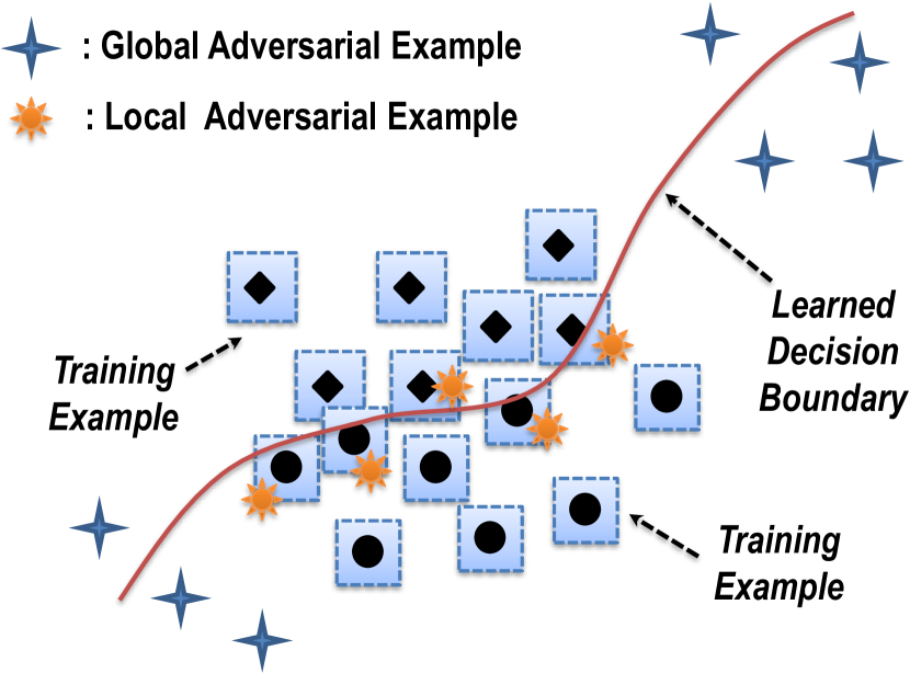
Figure 1: Global vs. local adversarial examples.

Loosely speaking, the maximum of $\mathcal{L}_{f}\left(\mathbf{x}_{1},\mathbf{x}_{2}\right)$ over the entire input space can serve as a measure of global model robustness. If it is larger than a preset threshold, the DNN may be deemed as vulnerable towards global adversarial attacks. On the other hand, (2) is a global optimization problem for which multiple near-optimal solutions may be reached by starting from different initial solutions or employing different optimization methods. Practically, any pair of two close inputs $\mathbf{x}_{1},\mathbf{x}_{2}$ with different model predictions in the case of classification or a sufficiently large value of $\mathcal{L}_{f}\left(\mathbf{x}_{1},\mathbf{x}_{2}\right)$ in the case of regression may be considered as a global adversarial example pair.

It is important to note that our problem formulation doesn’t restrict adversarial examples to be around a certain input example as in the case of the existing local adversarial attacks; it only sets an indistinguishable distance between a pair of two input examples in order to examine the entire input space, e.g. at locations far away from the training or testing dataset. Fig. 1 contrasts the conventional local adversarial examples with the proposed global adversarial examples. Importantly, our global attack formulation does not require additional labeled data; it directly measures the model’s sensitivity to input perturbation and be applied globally in the entirety of the input space.

We propose two families of attack methods to solve (2) as a way of generating global adversarial examples: 1) alternating gradient global adversarial attacks and 2) extreme-value-guided MCMC sampling global adversarial attack, as discussed in Section 3 and Section 4, respectively.

3 Alternating gradient global adversarial attacks

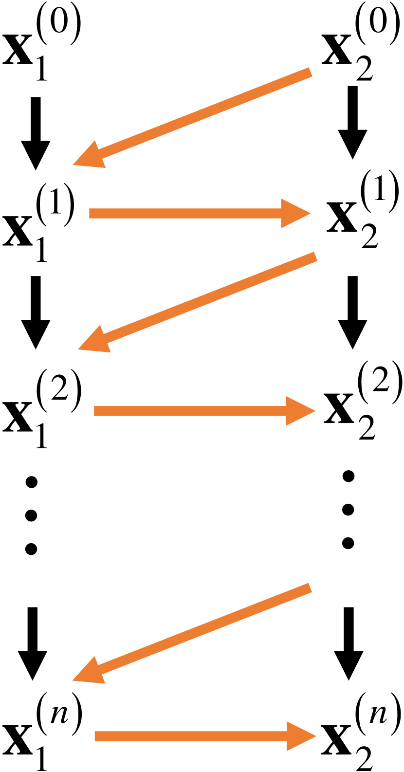
Figure 2: Alternating attack illustration.

For global adversarial example pair generation per (2), a pair of two examples $\left(\mathbf{x}_{1},\mathbf{x}_{2}\right)$ shall be be optimized to maximize the loss $\mathcal{L}_{f}\left(\mathbf{x}_{1},\mathbf{x}_{2}\right)$ under a distance constraint. We propose a family of attack methods called alternating gradient global adversarial attacks which proceed as follows: 1) start from an initial input pair; 2) fix the first example, and then attack (move) the second under the distance constraint while maximizing the loss $\mathcal{L}_{f}\left(\mathbf{x}_{1},\mathbf{x}_{2}\right)$ using a gradient-based local adversarial attack method, referred to as a sub-attack method here, 3) swap the roles of the first and (updated) second examples, i.e. fix the second example while attacking the first, 4) repeat this process for a number of iterations, as shown in Fig. 2.

Given a DNN model $f$ and a loss function $\mathcal{L}$, a sub-attack method can be characterized using a function $\mathbf{x}^{\prime}=f_{s\_attk}\left(\mathbf{x},y,\mathcal{R}_{\mathbf{x},\epsilon};f,\mathcal{L}\right)$ constructing an adversarial example $\mathbf{x}^{\prime}$ w.r.t example $\mathbf{x}$ and its corresponding label $y$, where $\mathcal{R}_{\mathbf{x},\epsilon}=\left\{\mathbf{x}+\delta|\left\|\delta\right\|\leq\epsilon\right\}$ specifies the region for adversarial sample generation. Suppose we start with an initial example pair $\left(\mathbf{x}_{1}^{\left(0\right)},\mathbf{x}_{2}^{\left(0\right)}\right)$, then we get the $\left(i+1\right)$-round example pair from the $\left(i\right)$-round sample pair by:

$$\mathbf{x}_{1}^{\left(i+1\right)} = f_{s\_attk}\left(\mathbf{x}_{1}^{\left(i\right)},f\left(\mathbf{x}_{2}^{\left(i\right)}\right),\mathcal{R}_{\mathbf{x}_{2}^{\left(i\right)},\epsilon};f,\mathcal{L}\right)$$ (3)

$$\mathbf{x}_{2}^{\left(i+1\right)} = f_{s\_attk}\left(\mathbf{x}_{2}^{\left(i\right)},f\left(\mathbf{x}_{1}^{\left(i+1\right)}\right),\mathcal{R}_{\mathbf{x}_{1}^{\left(i+1\right)},\epsilon};f,\mathcal{L}\right)$$ (4)

Here, to attack one example, we use the other example’s model prediction as the label when applying the sub-attack method $f_{s\_attk}$ so that the difference between two examples’ model predictions is maximized. In the meanwhile, the search region for attacking one example is constrained (centered) by the other example. Hence, the distance between the two examples is always less than $\epsilon$. Equations 3 and 4 are invoked to alternately attack $\mathbf{x}_{1}^{\left(i\right)}$ and $\mathbf{x}_{2}^{\left(i\right)}$ to generate an updated example pair for the next round. As the global attack continues, multiple global adversarial sample pairs may be generated along the way.

Algorithm 1 Global PGD attack algorithm for classification.

0:     Initial starting example pair $\left(\mathbf{x}_{1}^{\left(0\right)},\mathbf{x}_{2}^{\left(0\right)}\right)$; Example vector dimension $D$; distance constraint $\epsilon$; Number of total rounds $N$; Number of sub-attack steps $S$; Step size $a$ for the sub-attack.

0:     The set of generated global adversarial sample pairs $T$;

1:  $T=\left\{\right\}$

2:  for $i\leftarrow 1$ to $N$ do

3:     Sample a uniform distribution perturbation $\delta\sim\mathrm{U}\left[-\epsilon,\epsilon\right]^{D}$

4:     $\mathbf{x}_{1}^{\left(i\right)}\leftarrow Clip\left(\mathbf{x}_{1}^{\left(i-1\right)}+\delta,\mathcal{R}_{\mathbf{x}_{2}^{\left(i-1\right)},\epsilon}\right)$

5:     for $j\leftarrow 1$ to $S$ do

6:        $\mathbf{x}_{1}^{\left(i\right)}\leftarrow Clip\left(\mathbf{x}_{1}^{\left(i\right)}+a\cdot\mathrm{sign}\left(\nabla_{\mathbf{x}_{1}}\mathcal{L}_{f}\left(\mathbf{x}_{1}^{\left(i\right)},\mathbf{x}_{2}^{\left(i-1\right)}\right)\right),\mathcal{R}_{\mathbf{x}_{2}^{\left(i-1\right)},\epsilon}\right)$

7:     end for

8:     Sample a uniform distribution perturbation $\delta\sim\mathrm{U}\left[-\epsilon,\epsilon\right]^{D}$

9:     $\mathbf{x}_{2}^{\left(i\right)}\leftarrow Clip\left(\mathbf{x}_{2}^{\left(i-1\right)}+\delta,\mathcal{R}_{\mathbf{x}_{1}^{\left(i\right)},\epsilon}\right)$

10:     for $j\leftarrow 1$ to $S$ do

11:        $\mathbf{x}_{2}^{\left(i\right)}\leftarrow Clip\left(\mathbf{x}_{2}^{\left(i\right)}+a\cdot\mathrm{sign}\left(\nabla_{\mathbf{x}_{2}}\mathcal{L}_{f}\left(\mathbf{x}_{2}^{\left(i\right)},\mathbf{x}_{1}^{\left(i\right)}\right)\right),\mathcal{R}_{\mathbf{x}_{1}^{\left(i\right)},\epsilon}\right)$

12:     end for

13:     $T\leftarrow T\cup\left\{\left(\mathbf{x}_{1}^{\left(i\right)},\mathbf{x}_{2}^{\left(i\right)}\right)\right\}$

14:  end for

Choice of sub-attack methods.

We leverage the popular gradient-based local adversarial attack methods as sub-attack methods under the above family of global attacks. Particularly, the fast gradient sign method (FGSM) [3], iterative FGSM (IFGSM) [7], and projected gradient descent (PGD) [8] may be considered for sub-attack method $f_{s\_attk}$. As one example, we present the algorithm flow for the global PGD (G-PGD) attack targeting classifiers with PGD employed as the sub-attack in Algorithm 1, where the $Clip\left(\mathbf{x},mathcal{R}\right)$ function drags the input $\mathbf{x}$ outside the preset region $\mathcal{R}$ onto the boundary of $\mathcal{R}$. The global IFGSM (G-IFGSM) skips the random noise perturbations (steps 3 and 8). The global FGSM (G-FGSM) sets the number of sub-attack steps $S$ to be $1$ and the step size for sub-attack $a$ to be $\epsilon$ in addition to ignoring the random noise perturbation steps.

4 Extreme-value-guided MCMC sampling attack

While the family of alternating gradient global adversarial attacks discussed in Section 3 can work effectively in practice, such methods may get trapped at a local maximum, degrading the quality of global attack. To this end, we propose a stochastic optimization approach based on the extreme value distribution theory and Markov Chain Monte Carlo (MCMC) method, which is more advantageous from a global optimization point of view.

Extreme value distribution.

Consider sampling a set of i.i.d input example pairs $\left\{\left(\mathbf{x}_{1,1},\mathbf{x}_{2,1}\right),\cdots,\left(\mathbf{x}_{1,n},\mathbf{x}_{2,n}\right)\right\}$ in the input pair space $\Omega\times\Omega$. The greatest loss value $L^{*}=\max_{i\in\left[1,n\right]}\mathcal{L}_{f}\left(\mathbf{x}_{1,i},\mathbf{x}_{2,i}\right)$ can be regarded as a random variable following a certain distribution characterized by its density function $p_{L^{*}}\left(l\right)$. The Fisher-Tippett-Gnedenko theorem says that the distribution of the maximum value of examples, if exists, can only be one of the three families of extreme value distribution: the Gumbel class, the Fréchet and the reverse Weibull class [15]. Hence, $p_{L^{*}}\left(l\right)$ falls into one of the three families as well, whose cumulative density function (CDF) $F_{L^{*}}\left(l\right)$ can be written in a unified form, called the generalized extreme value (GEV) distribution:

$$F_{L^{*}}\left(l\right)=\left\{\begin{array}[]{ll}\exp\left(-\left(1+\xi\frac{l-\mu}{\sigma}\right)^{-1/\xi}\right)&\xi\neq 0\\ \exp\left(-\exp\left(-\frac{l-\mu}{\sigma}\right)\right)&\xi=0\end{array}\right.$$ (5)

where $\mu$, $\sigma$ and $\xi$ are the location, scale, and shape parameter for the GEV distribution and may be obtained through the maximum likelihood estimation (MLE).

Assuming that the desired generalized extreme value (GEV) distribution of the loss function is available, multiple large loss values, corresponding to potential global adversarial example pairs, may be generated by sampling the GEV distribution. The added benefit here is that the inherent randomness in this sampling process may be explored to find more globally optimal solutions. Nevertheless, since the GEV distribution may not be easily sampled directly, We adopt the Markov Chain Monte Carlo (MCMC) method to sample the GEV distribution [16]. In reality, the GEV distribution is not known a priori and shall be estimated using MLE based on a sample of data as described below.

Extreme-value-guided MCMC sampling algorithm (GEVMCMC).

The proposed GEVMCMC algorithm is shown in Algorithm 2 for the case of classification problems. There exist two essential components for MCMC sampling: the target distribution, which is in this case the desired GEV distribution, and the proposal distribution, which is a surrogate distribution easy to sample. For each MCMC round, we collect an example from the proposal distribution, and then accept this example or discard it while keeping the previous one based on an acceptance ratio $p_{A}$ in Step 6 of Algorithm 2 [16]. In order to sample the block maximum for the extreme value distribution, a block of example pairs are collected from the proposal distribution in each round as in Step 3 of the algorithm instead of a single example. As the MCMC sampling process proceeds, the actual sampling distribution implemented converges to the target (GEV) distribution.

Algorithm 2 Extreme-value-guided MCMC sampling algorithm (GEVMCMC) for global attack.

0:     Initial starting example pair $\left(\mathbf{x}_{1}^{\left(0\right)},\mathbf{x}_{2}^{\left(0\right)}\right)$; Number of total rounds $N$; Number of warm-up rounds $N_{w}$; Block size $B$; Number of example pairs $k$ used for GEV distribution update;

0:     The set of the generated global adversarial example pairs $T$;

1:  Apply G-PGD for $N_{w}$ rounds to warm-up and update T.

2:  for $i\leftarrow N_{w}+1$ to $N$ do

3:     Sample $B$ i.i.d. samples $\left\{\left(\mathbf{x}_{1}^{\left[1\right]},\mathbf{x}_{2}^{\left[1\right]}\right),\cdots,\left(\mathbf{x}_{1}^{\left[B\right]},\mathbf{x}_{2}^{\left[B\right]}\right)\right\}$ from the proposal distribution $q\left(\mathbf{x}_{1},\mathbf{x}_{2}|\mathbf{x}_{1}^{\left(i-1\right)},\mathbf{x}_{2}^{\left(i-1\right)}\right)$

4:     $\left(\mathbf{x}_{1}^{*},\mathbf{x}_{2}^{*}\right)\leftarrow\operatorname*{argmax}_{j\in\left[1,B\right]}\mathcal{L}_{f}\left(\mathbf{x}_{1}^{\left[j\right]},\mathbf{x}_{2}^{\left[j\right]}\right)$

5:     Update the GEV distribution $p_{L^{*}}\left(l\right)$ using top $k$ loss values in the history.

6:     $p_{A}\leftarrow\min\left\{1.0,\frac{p_{L^{*}}\left(\mathcal{L}_{f}\left(\mathbf{x}_{1}^{*},\mathbf{x}_{2}^{*}\right)\right)q\left(\mathbf{x}_{1}^{\left(i-1\right)},\mathbf{x}_{2}^{\left(i-1\right)}|\mathbf{x}_{1}^{*},\mathbf{x}_{2}^{*}\right)}{p_{L^{*}}\left(\mathcal{L}_{f}\left(\mathbf{x}_{1}^{\left(i-1\right)},\mathbf{x}_{2}^{\left(i-1\right)}\right)\right)q\left(\mathbf{x}_{1}^{*},\mathbf{x}_{2}^{*}|\mathbf{x}_{1}^{\left(i-1\right)},\mathbf{x}_{2}^{\left(i-1\right)}\right)}\right\}$

7:     Sample a uniform random variable $\alpha\sim\mathrm{U}\left[0,1\right]$

8:     if $\alpha\leq p_{A}$ then

9:        Accept the new example. $\left(\mathbf{x}_{1}^{\left(i\right)},\mathbf{x}_{2}^{\left(i\right)}\right)=\left(\mathbf{x}_{1}^{*},\mathbf{x}_{2}^{*}\right)$

10:     else

11:        Reject and keep the previous example. $\left(\mathbf{x}_{1}^{\left(i\right)},\mathbf{x}_{2}^{\left(i\right)}\right)=\left(\mathbf{x}_{1}^{\left(i-1\right)},\mathbf{x}_{2}^{\left(i-1\right)}\right)$

12:     end if

13:     $T\leftarrow T\cup\left\{\left(\mathbf{x}_{1}^{\left(i\right)},\mathbf{x}_{2}^{\left(i\right)}\right)\right\}$

14:  end for

Importantly, the generalized extreme value (GEV) distribution $p_{L^{*}}\left(l\right)$ of the loss function doesn’t exist at the beginning of the algorithm. Therefore, it is estimated during the sampling process. Two techniques are considered to obtain an accurate GEV distribution. A warm-up procedure (Step 1 in Algorithm 2) using a few rounds of G-PGD is performed first to collect a few global adversarial example pairs of large loss values. In each round, the top k loss values among all example pairs in the history including the ones in the current block are selected to estimate $p_{L^{*}}\left(l\right)$ based on MLE in Step 5 of Algorithm 2.

Proposal distribution design.

The convergence speed of MCMC sampling towards the target distribution critically depends on the proposal distribution [16]. To efficiently generate high-quality global adversarial example pairs, we consider the following essential aspects in designing the proposal distribution: (1) finding large loss values; (2) enabling global search; (3) constraining two examples in each pair to be within distance $\epsilon$.

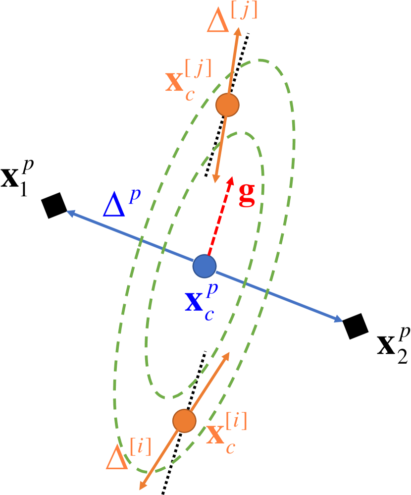
Figure 3: MCMC proposal distribution design illustration.

We decompose the sampling of an example pair into two sequential steps: sample the center location $\mathbf{x}_{c}$ and sample the difference vector $\Delta$ between the two examples. Then, we construct the example pair by $\mathbf{x}_{1}=\mathbf{x}_{c}+\Delta,\mathbf{x}_{2}=\mathbf{x}_{c}-\Delta$, as shown in Fig. 3. The two sampling steps are independent of each other, and hence, the proposal distribution conditioning on the previous example pair $\left(\mathbf{x}_{c}^{p},\Delta^{p}\right)$ is split into a product of a center proposal and difference proposal distribution:

$$q\left(\mathbf{x}_{c},\Delta|\mathbf{x}_{c}^{p},\Delta^{p}\right)=q_{x^{c}}\left(\mathbf{x}_{c}|\mathbf{x}_{c}^{p},\Delta^{p}\right)q_{\Delta}\left(\Delta|\mathbf{x}_{c}^{p},\Delta^{p}\right).$$ (6)

As such, the distance constraint for the two examples is only taken into consideration in the design of $q_{\Delta}\left(\Delta|\mathbf{x}_{c}^{p},\Delta^{p}\right)$ and no distance constraint is necessary when sampling the center.

We speed up the convergence of MCMC by incorporating the (normalized) gradient information

$$\mathbf{g}=\frac{\nabla_{\mathbf{x}_{c}}\mathcal{L}_{f}\left(\mathbf{x}_{c}^{p}+\Delta^{p},\mathbf{x}_{c}^{p}-\Delta^{p}\right)}{\left|\nabla_{\mathbf{x}_{c}}\mathcal{L}_{f}\left(\mathbf{x}_{c}^{p}+\Delta^{p},\mathbf{x}_{c}^{p}-\Delta^{p}\right)\right|}$$ (7)

into the proposal distribution design. We design the center proposal distribution to be a multi-variate Gaussian distribution centered at $\mathbf{x}_{c}^{p}$ with a covariance matrix biasing to sampling along the gradient direction $\mathbf{g}$ to increase the likelihood of finding large loss values while allowing sampling in other directions during the same time:

$$q_{x^{c}}\left(\mathbf{x}_{c}|\mathbf{x}_{c}^{p},\Delta^{p}\right)=\mathcal{N}\left(\mathbf{x}_{c}^{p},\lambda_{0}^{2}\mathbf{I}+\left(\lambda_{m}^{2}-\lambda_{0}^{2}\right)\mathbf{g}\mathbf{g}^{\mathrm{T}}\right),$$ (8)

where $\lambda_{m}^{2}$ sets the largest eigenvalue and $\lambda_{0}^{2}<\lambda_{m}^{2}$ sets all other eigenvalues of the covariance matrix. The absolute values of $\lambda_{0}$ and $\lambda_{m}$ control the size of the search region while the ratio between $\lambda_{m}$ and $\lambda_{0}$ determines to what extent we want to focus on the gradient direction.

The gradient sign information is incorporated into the difference proposal distribution considering the distance constraint $\epsilon$. Particularly, for the $l_{\infty}$ norm based distance measure, we propose a Bernoulli distribution with parameter $p_{B}>0.5$ for each element of the difference vector:

$$\Delta_{i}=\left\{\begin{array}[]{ll}\frac{\epsilon}{2}\mathrm{sign}\left(g_{i}\right)&\textrm{with probability $p_{B}$}\\ -\frac{\epsilon}{2}\mathrm{sign}\left(g_{i}\right)&\textrm{with probability $1-p_{B}$},\end{array}\right.$$ (9)

which ensures that the pair $\left(\mathbf{x}_{1},\mathbf{x}_{2}\right)$ be within distance $\epsilon$ and each difference component is more likely to be set according to the corresponding gradient sign component.

5 Experimental results

Experimental settings.

We investigate several local and global methods on two popular image classification datasets: MNIST [17] and CIFAR10 [18]. To evaluate DNN robustness globally in the input space, we create an additional class “meaningless” and append 6,000 and 5,000 random noisy images (one tenth of the original training dataset) under this “meaningless” class into the original MNIST and CIFAR10 training datasets, respectively, and refer to the expanded training datasets as the augmented training datasets. All trained DNNs perform classification across 11 classes.

For MNIST, we train a neural network with two convolutional and two fully-connected layers with an accuracy of $99.43\%$ with 40 training epochs. For CIFAR10, a VGG16 [19] network is trained for 300 epochs, reaching $94.25\%$ accuracy. Furthermore, we globally attack adversarially-trained models, which are trained using adversarial training based on local adversarial examples. In each epoch of adversarial training, the adversarial samples are generated by attacking the DNN model from the last epoch using a 30-step local white-box PGD attack, which is considered a strong first-order attack [8]. And then an updated model is trained using both the augmented training set and the generated adversarial images. Adversarial training process is performed for additional 40 epochs for the MNIST model and 30 epochs for the CIFAR10 model, respectively. The ratio of the weighting parameters between the losses of the examples in the augmented training set and adversarial examples are $1:1$.

Adversarial attack parameter settings.

The $l_{\infty}$ norm based perturbation limit (the maximum allowed difference between two close images) is set to $\epsilon_{MNIST}=0.1$ for MNIST and to $\epsilon_{CIFAR10}=0.005$ for CIFAR10. We add another 10,000 random images with the “meaningless” class label into the original testing dataset (10,000 samples) to create an augmented testing dataset. We experiment three common local adversarial attack methods: FGSM [3], IFGSM [7], and PGD [8], referred to as L-FGSM, L-IFGSM and L-PGD in this paper. Both L-IFGSM and L-PGD perform a 30-step attack with a $l_{\infty}$ step size of $\epsilon/10$. All local attacks are performed on the augmented testing set.

All four proposed global adversarial attack methods are considered: alternating gradient global adversarial attack with different sub-attack methods of FGSM (G-FGSM), IFGSM(G-IFGSM) and PGD (G-PGD); extreme-value-guided sampling global attack (GEVMCMC). For all global attack methods, we randomly pick 100 images from the original testing dataset and from the appended random testing dataset, respectively, to form the first images of the 100 starting pairs. The second image of each pair is obtained by adding small uniformly-distributed random noise bounded by perturbation size $\epsilon$ to the first image. 100 rounds of optimization are performed by all global adversarial attack methods, generating a two sets of 10,000 adversarial example pairs, one set for each of the two starting conditions: start with the 100 original testing images, start from the 100 appended random testing images. G-IFGSM and G-PGD share the same parameter settings with their local attack counterparts L-IFGSM and L-PGD, respectively. The number of GEVMCMC initial G-PGD warm-up rounds is 10 for MNIST and 30 for CIFAR10. The block size $B$ is set to be 59. Three parameters for the proposal distribution for MNIST are $\lambda_{m}=1.2\epsilon_{MNIST},\lambda_{0}=0.3\epsilon_{MNIST},p_{B}=0.95$, and for CIFAR10 they are set to be $\lambda_{m}=4.8\epsilon_{CIFAR10},\lambda_{0}=0.6\epsilon_{CIFAR10},p_{B}=0.99$.

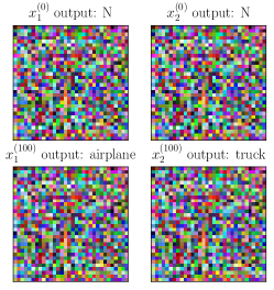
(a)

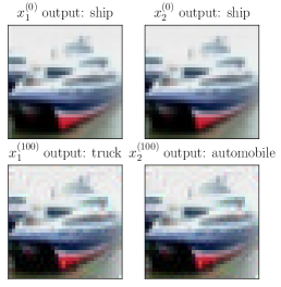
(b)

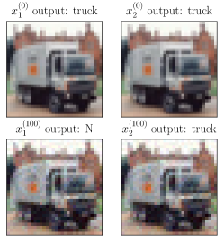
(c)

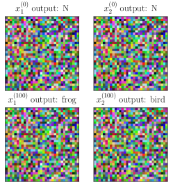
(d)

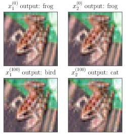
(e)

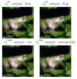
(f)

Figure 4: Global adversarial sample pairs for the CIFAR10 model generated by GEVMCMC.

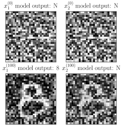
(a)

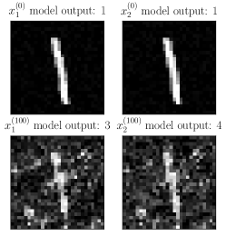
(b)

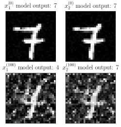
(c)

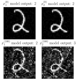
(d)

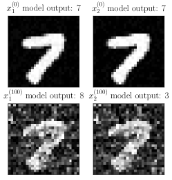
(e)

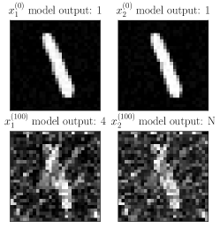
(f)

Figure 5: Global adversarial sample pairs for the MNIST model generated by GEVMCMC.

Generated global adversarial sample pairs.

The proposed global adversarial attack methods can generate diverse global adversarial pairs which are rather different from typical local attacks, representing a new type of DNN vulnerability. Fig. 4 and Fig. 5 show a set of global adversarial example pairs generated by GEVMCMC for the two datasets. In each sub-figure, the two images on the top are the starting pair of two identical starting images. The two at the bottom are the final global adversarial pair generated after 100 rounds of optimization steps. “N" indicates that the class label predicated by the model is “meaningless".

Compared to standard local adversarial attacks, the proposed global adversarial pairs are much more diverse and intriguing. For instance, it is possible to start with two identical random meaningless image but end up with some other two random images that are very similar to each other but have different legitimate class labels predicted by the model such as ones in Fig. 4a and 4d. We can also start from two identical images of a legitimate predicted class, and end up with two images with predicated labels that are different from each other and are also different from the starting label, as shown in Fig. 4b, 4e, 4f, 5b and 5e. Clearly, the existing local attacks such as FGSM, IFGSM, and PGD are not able to generate such complex global adversarial scenarios, which reveal additional hidden vulnerabilities of the model.

Importantly, the existing local adversarial attacks cannot explore the input space beyond the training or testing dataset due to the perturbation constraint. In contrast, the proposed global adversarial attacks are very appealing in the following way: they may find a path towards unseen input space and check the model robustness along the way. For instance, we may start from some random testing image (Fig. 5a) or original testing image (Fig. 5c), and end up with a completely different image pair which may be both recognized by the humans as a legitimate class, however, the model predicts different labels for them. For instance, the final pairs in the Fig. 5a and Fig. 5c may be recognized as “8" and “4", respectively, which are completely different from their starting label.

Table 1: Natural MNIST model (w/o local adversarial training) adversarial attack results.

Method	Start from Original Test Image			Start from Random Test Image
	Attack Rate	Max Loss	Avg. Loss	Attack Rate	Max Loss	Avg. Loss
L-FGSM	18.18%	20.94	0.77	5.82%	6.43	0.16
L-IFGSM	29.80%	21.76	1.17	51.96%	7.64	1.18
L-PGD	29.59%	21.73	1.16	49.44%	7.57	1.13
G-FGSM	99.14%	23.40	10.78	99.01%	20.04	9.62
G-IFGSM	99.92%	22.21	9.19	100.00%	12.05	5.94
G-PGD	99.94%	20.44	10.18	100.00%	11.94	6.58
GEVMCMC	99.93%	24.93	14.91	100.00%	19.98	12.67

Table 2: Adversarially-trained MNIST model adversarial attack results.

Method	Start from Original Test Image			Start from Random Test Image
	Attack Rate	Max Loss	Avg. Loss	Attack Rate	Max Loss	Avg. Loss
L-FGSM	3.28%	15.14	0.11	0.00%	0.00	0.00
L-IFGSM	3.89%	15.56	0.13	0.00%	0.06	0.00
L-PGD	3.88%	15.57	0.13	0.00%	0.05	0.00
G-FGSM	98.07%	17.79	8.19	97.50%	19.09	7.63
G-IFGSM	99.47%	14.25	7.84	99.56%	17.81	11.43
G-PGD	99.50%	18.08	8.61	99.58%	19.59	12.07
GEVMCMC	99.38%	18.28	9.91	99.55%	18.06	12.04

Table 3: Natural CIFAR10 model (w/o local adversarial training) adversarial attack results.

Method	Start from Original Test Image			Start from Random Test Image
	Attack Rate	Max Loss	Avg. Loss	Attack Rate	Max Loss	Avg. Loss
L-FGSM	26.77%	11.42	1.90	0.00%	0.01	0.00
L-IFGSM	44.80%	12.06	3.58	0.00%	0.02	0.00
L-PGD	43.92%	12.04	3.51	0.00%	0.02	0.00
G-FGSM	95.96%	12.75	8.72	95.15%	11.10	5.48
G-IFGSM	99.68%	12.90	11.02	98.36%	10.76	6.45
G-PGD	99.71%	13.55	11.30	98.33%	11.02	6.70
GEVMCMC	99.58%	13.18	8.94	98.37%	11.02	7.18

Table 4: Adversarially-trained CIFAR10 model adversarial attack results.

Method	Start from Original Test Image			Start from Random Test Image
	Attack Rate	Max Loss	Avg. Loss	Attack Rate	Max Loss	Avg. Loss
L-FGSM	19.29%	10.97	0.83	0.00%	0.00	0.00
L-IFGSM	21.25%	11.03	0.92	0.00%	0.00	0.00
L-PGD	21.19%	11.03	0.92	0.00%	0.00	0.00
G-FGSM	95.29%	9.62	4.11	90.47%	6.57	2.52
G-IFGSM	98.23%	9.83	4.60	95.85%	6.99	2.94
G-PGD	98.26%	10.54	4.77	95.88%	6.97	3.03
GEVMCMC	98.25%	10.89	5.47	95.89%	6.66	3.67

Local vs. global adversarial attacks

Table 1-4 show the global adversarial attack results for the MNIST and CIFAR10 models without and with local adversarial training. If the model predictions for the two examples in a generated global adversarial pair are different, we regard this pair as one successful global attack. In these tables, the attack rate is defined as the ratio between the successful number of attacks over the total number of trails which is 10,000. The Max loss and Avg. loss are the maximum loss and average loss found in the attack process.

Attacking the natural MNIST and CIFAR10 models using a local attack method can reach a reasonablly high attack rate. For instance, L-PGD has an attack rate of $29.59\%$ in the case of the natural MNIST, which drops down to $3.88\%$ for the case of the adversarially-trained MNIST model, showing that adversarial training using local adversarial examples does improve the defense to such local attacks. However, all global adversarial attack methods achieve almost 100.00% attack rate and produce much higher average loss values compared to the local attack methods, regardless whether local adversarial training is performed or not. It is evident that adversarial training based on local adversarial examples shows none or little defense to global attacks. This indicates the effectiveness of the proposed global attack methods, and equally importantly, suggests that global adversarial examples defined in this paper must be coped with when training robust DNN models.

Table 5: Comparison between GEVMCMC and other proposed global attacks when starting from the same 100 original test (“Test") or 100 random testing (“Rand") example pairs. Each entry shows the number of cases out of the total 100 cases where the final adversarial pair generated by GEVMCMC has a loss higher than the one generated by the other method.

Method	MNIST				CIFAR10
	Natural		Adv.-Trained		Natural		Adv.-Trained
	Test	Rand	Test	Rand	Test	Rand	Test	Rand
G-FGSM	86	95	69	81	33	72	76	67
G-IFGSM	98	100	92	90	69	85	84	92
G-PGD	97	100	80	67	12	73	74	90

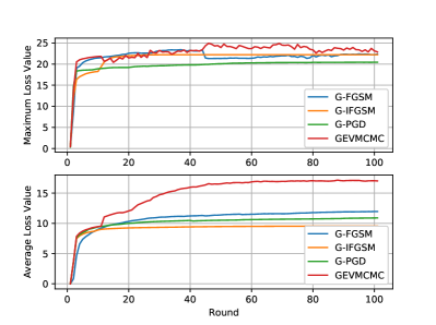
(a) Testing image starting image pair

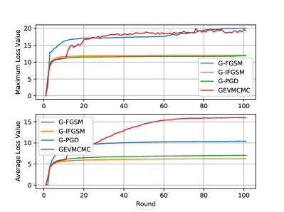
(b) Random image starting image pair

Figure 6: Loss value found by global adversarial attack in each round for the natural MNIST model.

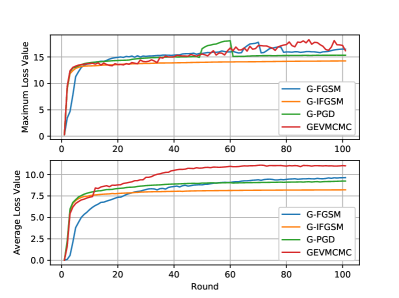
(a) Testing image starting image pair

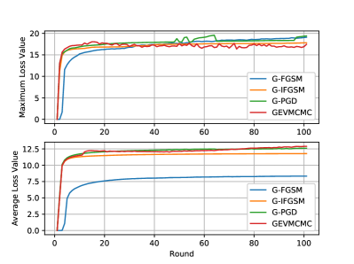
(b) Random image starting image pair

Figure 7: Loss value found by global adversarial attack in each round for the adversarially-trained MNIST model.

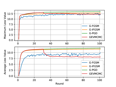
(a) Testing image starting image pair

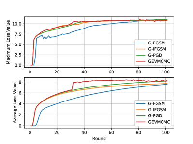
(b) Random image starting image pair

Figure 8: Loss value found by global adversarial attack in each round for the natural CIFAR10 model.

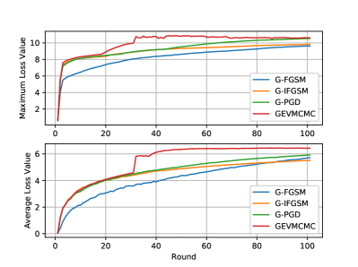
(a) Testing image starting image pair

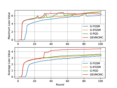
(b) Random image starting image pair

Figure 9: Loss value found by global adversarial attack in each round for the adversarially-trained CIFAR10 model.

Comparison of the proposed global adversarial attack methods

Table 5 compares the two types of the proposed global attack methods when starting from the same 100 original test (“Test") or 100 random testing (“Rand") example pairs. Each entry shows the number of cases out of the total 100 cases where the final adversarial pair generated by GEVMCMC has a loss higher than the one generated by the other method. Most entries in the table are larger than 50, implying that GEVMCMC finds worse adversarial example pairs than other global adversarial attack methods. We further show the maximum loss value and average loss value of the adversarial example pairs in each round in Fig. 6 - 9. After the initial warm-up rounds using G-PGD, the loss found by GEVMCMC increases rapidly, and ends up with a much larger value compared to that of the other global adversarial attack methods, which tend to converge at a local maximum. The only case in which GEVMCMC does not beat other global adversarial attack methods is the attacking of the natural CIFAR10 model starting with the original testing images, showing the overall better effectiveness of GEVMCMC.

6 Conclusion

We propose a new global adversarial example pair concept and formulate the corresponding global adversarial attack problem to assess the robustness of DNNs over the entire input space without human data labeling. We further propose two families of global adversarial attack methods: (1) alternating gradient global adversarial attacks and (2) extreme-value-guided MCMC sampling global attack (GEVMCMC), demonstrating that DNN models even trained with local adversarial training are vulnerable to this new type of global attacks. Our attack methods are able to generate diverse and intriguing global adversarial which are very different from typical local attacks and shall be taken into consideration when training a robust model. GEVMCMC demonstrates the overall best performance among all proposed global attack methods due to its probabilistic nature.

References

- Luckow et al. [2016] Andre Luckow, Matthew Cook, Nathan Ashcraft, Edwin Weill, Emil Djerekarov, and Bennie Vorster. Deep learning in the automotive industry: applications and tools. In IEEE International Conference on Big Data, 2016.
- Carrio et al. [2017] Adrian Carrio, Carlos Sampedro, Alejandro Rodriguez-Ramos, and Pascual Campoy. A review of deep learning methods and applications for unmanned aerial vehicles. Journal of Sensors, 2017.
- Goodfellow et al. [2015] Ian Goodfellow, Jonathon Shlens, and Christian Szegedy. Explaining and harnessing adversarial examples. In International Conference on Learning Representations, 2015.
- Moosavi-Dezfooli et al. [2017] Seyed-Mohsen Moosavi-Dezfooli, Alhussein Fawzi, Omar Fawzi, Pascal Frossard, and Stefano Soatto. Analysis of universal adversarial perturbations. arXiv preprint arXiv:1705.09554, 2017.
- Papernot et al. [2016] Nicolas Papernot, Patrick McDaniel, Somesh Jha, Matt Fredrikson, Z. Berkay Celik, and Ananthram Swami. The limitations of deep learning in adversarial settings. In IEEE European Symposium on Security and Privacy, 2016.
- Carlini and Wagner [2016] Nicholas Carlini and David Wagner. Towards evaluating the robustness of neural networks. arXiv preprint arXiv:1608.04644, 2016.
- Kurakin et al. [2016] Alexey Kurakin, Ian Goodfellow, and Samy Bengio. Adversarial machine learning at scale. arXiv preprint arXiv:1611.01236, 2016.
- Madry et al. [2018] Aleksander Madry, Aleksandar Makelov, Ludwig Schmidt, Dimitris Tsipras, and Adrian Vladu. Towards deep learning models resistant to adversarial attacks. In International Conference on Learning Representations, 2018.
- Weng et al. [2018] Tsui-Wei Weng, Huan Zhang, Pin-Yu Chen, Jinfeng Yi, Dong Su, Yupeng Gao, Cho-Jui Hsieh, and Luca Daniel. Evaluating the robustness of neural networks: An extreme value theory approach. In International Conference on Learning Representations, 2018.
- Tsuzuku et al. [2018] Yusuke Tsuzuku, Issei Sato, and Masashi Sugiyama. Lipschitz-margin training: scalable certification of perturbation invariance for deep neural networks. In International Conference on Neural Information Processing Systems, 2018.
- Goodfellow [2018] Ian J. Goodfellow. Gradient masking causes CLEVER to overestimate adversarial perturbation size. arXiv preprint arXiv:1804.07870, 2018.
- Huster et al. [2018] Todd Huster, Cho-Yu Jason Chiang, and Ritu Chadha. Limitations of the lipschitz constant as a defense against adversarial examples. arXiv preprint arXiv:1807.09705, 2018.
- Song et al. [2018] Yang Song, Rui Shu, Nate Kushman, and Stefano Ermon. Constructing unrestricted adversarial examples with generative models. In International Conference on Neural Information Processing Systems, 2018.
- Dunn et al. [2019] Isaac Dunn, Tom Melham, and Daniel Kroening. Generating realistic unrestricted adversarial inputs using dual-objective GAN training. arXiv preprint arXiv:1905.02463, 2019.
- Gomes and Guillou [2015] M. Ivette Gomes and Armelle Guillou. Extreme value theory and statistics of univariate extremes: a review. International Statistical Review, 2015.
- Andrieu et al. [2003] Christophe Andrieu, Nando de Freitas, Arnaud Doucet, and Michael I. Jordan. An introduction to mcmc for machine learning. Machine Learning, 2003.
- LeCun et al. [1998] Yann LeCun, Léon Bottou, Yoshua Bengio, and Patrick Haffner. Gradient-based learning applied to document recognition. Proceedings of the IEEE, 1998.
- Krizhevsky and Hinton [2009] Alex Krizhevsky and Geoffrey Hinton. Learning multiple layers of features from tiny images. Technical report, Citeseer, 2009.
- Simonyan and Zisserman [2014] Karen Simonyan and Andrew Zisserman. Very deep convolutional networks for large-scale image recognition. arXiv preprint arXiv:1409.1556, 2014.