QCD evolution of the orbital angular momentum of quarks and gluons:
Genuine twist-three part

Abstract

We present the numerical solution of the one-loop QCD evolution equation for the genuine twist-three part of the orbital angular momentum (OAM) distributions of quarks and gluons inside a longitudinally polarized nucleon. This is based on the observation that the evolution is identical to that of the Efremov-Teryaev-Qiu-Sterman function for transverse single spin asymmetry. Together with the known evolution of the Wandzura-Wilczek part, the one-loop evolution of OAM distributions is now practically under control. We also study, for the first time, the scale dependence of the potential angular momentum defined as the difference between the Ji and Jaffe-Manohar definitions of OAM.

I Introduction

After more than a decade of experimental programs at RHIC, HERMES, COMPASS and JLab Adare:2008aa ; Airapetian:2010ac ; Adamczyk:2012qj ; Alekseev:2010ub ; Adamczyk:2014ozi ; Prok:2014ltt , and concurrent theoretical efforts based on global QCD analysis deFlorian:2014yva ; Nocera:2014gqa ; Sato:2016tuz , we now know that the gluon helicity contribution $\Delta G$ to the Jaffe-Manohar sum rule of the nucleon spin Jaffe:1989jz

$$\frac{1}{2}=\frac{1}{2}\Delta\Sigma+\Delta G+L_{q}+L_{g}\,,$$ (1)

is nonzero and can be significant. Together with the well-known quark helicity contribution $\Delta\Sigma$, the first two terms of (1) account for $\sim 70\%$ of the total spin, leaving some room for the orbital angular momentum (OAM) $L_{q,g}$ of quarks and gluons. However, this is at best a tentative conclusion. The present estimate of $\Delta G$ is based on the RHIC 200 GeV $pp$ data which can only access a limited range of the Bjorken variable $x$. Uncertainties coming from the small $x$-region $x\lesssim 0.05$ are estimated to be huge, and might completely alter the current estimates. In such circumstances, an obvious direction to proceed for the QCD spin community is to better constrain $\Delta G(x)$ in the small-$x$ region. Indeed, new data from RHIC 510 GeV $pp$ runs have just begun to appear Adam:2019aml . Moreover, the precise determination of $\Delta G$ has been designated as one of the primary goals of the future Electron-Ion Collider (EIC) Accardi:2012qut .

An equally obvious direction is to directly constrain the OAM contributions $L_{q,g}$. Unfortunately, however, this is currently not pursued experimentally due to the lack of clean observables from which one can systematically extract $L_{q,g}$ as the moment of the corresponding $x$-distributions $L_{q,g}=\int_{0}^{1}dxL_{q,g}(x)$. In fact, it is only relatively recently that the rigorous definitions of $L_{q,g}(x)$ have been derived Hatta:2012cs (following the earlier developments Lorce:2011kd ; Hatta:2011ku ; Lorce:2011ni ), although their gauge non-invariant versions have been known for quite some time Harindranath:1998ve ; Hagler:1998kg . Such a progress has finally led theorists to identify a few experimental processes that are sensitive to $L_{q,g}(x)$ Courtoy:2013oaa ; Ji:2016jgn ; Hatta:2016aoc ; Bhattacharya:2017bvs ; Bhattacharya:2018lgm . In these works, observables have been computed to leading order, whereas a realistic global analysis requires the knowledge of the next-to-leading order (NLO) corrections together with the ‘DGLAP’ equation for $L_{q,g}(x)$ to NLO, or at least to leading order.

However, so far the evolution of $L_{q,g}(x)$ has not been fully understood even to leading order. This is because $L_{q}(x)$ and $L_{g}(x)$ are not the usual twist-two parton distribution functions (PDFs). They consist of the Wandzura-Wilczek (WW) part and the genuine twist-three part

$$L_{q,g}(x)=L_{q,g}^{WW}(x)+L_{3q,3g}(x)\,.$$ (2)

The WW part is related to the twist-two unpolarized and polarized PDFs. As such, its evolution is known to the same order as that of the corresponding twist-two distributions (namely, to three-loops). The LO evolution equation derived in the early literature Harindranath:1998ve ; Hagler:1998kg can be fully understood in this way Hoodbhoy:1998yb ; Boussarie:2019icw . More recently, the small-$x$ behavior of the WW part has received a lot of attention, mainly motivated by the aforementioned uncertainties of $\Delta G$ at small-$x$ Hatta:2018itc ; More:2017zqp ; Kovchegov:2019rrz ; Boussarie:2019icw . An analysis based on the double logarithmic resummation Boussarie:2019icw has shown that there is a significant cancellation between $\Delta G(x)$ and $L_{g}(x)$ in the small-$x$ region (see, however, Kovchegov:2019rrz ).

On the other hand, the genuine twist-three part $L_{3q,3g}(x)$ is given by the matrix elements of three-parton ($q\bar{q}g,ggg$), twist-three operators. The QCD evolution of such twist-three correlators is complicated even to one-loop, and to our knowledge, it has never been discussed in the context of OAM. Fortunately, however, it has been discussed in a different context—QCD evolution for the Efremov-Teryaev-Qiu-Sterman (ETQS) function Efremov:1984ip ; Qiu:1991wg for transverse single spin asymmetry Kang:2008ey ; Vogelsang:2009pj ; Braun:2009mi . Moreover, a C++ program to numerically solve this evolution has been developed by Pirnay Pirnay:2013fra . These results can be adapted for the present purpose with appropriate modifications. Thus, the goal of this paper is to articulate the evolution equation for $L_{3q,3g}(x)$ and demonstrate the feasibility of numerically solving this equation.

The paper is organized as follows: In Sec. II we will explain the quark and gluon OAM distributions and their evolutions. Then in Sec. III the evolution of the genuine twist-three part will be discussed. We will show numerical results on the evolution of the genuine twist-three part in Sec. IV. We will discuss the cusp anomalous dimensions for the large-$n$ moments and the scale dependence of the potential angular momentum. Finally, conclusions will be drawn in Sec. V.

II OAM distributions and their evolution equation

In this section, we first review the formula (2) derived in Hatta:2012cs and then discuss its evolution equation. We employ the following normalization for the singlet quark (and antiquark) OAM distribution $L_{q}(x)=\sum_{f}(L_{f}(x)+L_{\bar{f}}(x))$ and the gluon OAM distribution $L_{g}(x)$

$$L_{q}=\int_{0}^{1}dxL_{q}(x),\qquad L_{g}=\int_{0}^{1}dxL_{g}(x)\,.$$ (3)

Our normalization here is different from the one in Hatta:2012cs , but it is the same as in Hatta:2018itc ; Boussarie:2019icw . In the present normalization and notation, the result of Hatta:2012cs reads

$$L_{q}(x) = x\int^{1}_{x}\frac{dx^{\prime}}{x^{\prime}}(\Sigma(x^{\prime})+E_{q}(x^{\prime}))-x\int^{1}_{x}\frac{dx^{\prime}}{x^{\prime 2}}\Delta\Sigma(x^{\prime})$$ (4)

$$-x\int^{1}_{x}dx_{1}\int_{-1}^{1}dx_{2}\left(\Phi_{F}(x_{1},x_{2})-\Phi_{F}(-x_{1},-x_{2})\right){\cal P}\frac{3x_{1}-x_{2}}{x_{1}^{2}(x_{1}-x_{2})^{2}}$$

$$-x\int^{1}_{x}dx_{1}\int_{-1}^{1}dx_{2}\left(\widetilde{\Phi}_{F}(x_{1},x_{2})-\widetilde{\Phi}_{F}(-x_{1},-x_{2})\right){\cal P}\frac{1}{x_{1}^{2}(x_{1}-x_{2})}\,,$$

$$L_{g}(x) = x\int^{1}_{x}\frac{dx^{\prime}}{x^{\prime}}(G(x^{\prime})+E_{g}(x^{\prime}))-2x\int^{1}_{x}\frac{dx^{\prime}}{x^{\prime 2}}\Delta G(x^{\prime})$$ (5)

$$+2x\int^{1}_{x}\frac{dx^{\prime}}{x^{\prime 3}}\int dX(\Phi_{F}(x_{1},x_{2})-\Phi_{F}(-x_{1},-x_{2}))$$

$$+4x\int^{1}_{x}dx_{1}\int^{1}_{-1}dx_{2}\widetilde{M}_{F}(x_{1},x_{2}){\cal P}\frac{1}{x_{1}^{3}(x_{1}-x_{2})}$$

$$+4x\int^{1}_{x}dx_{1}\int^{1}_{-1}dx_{2}M_{F}(x_{1},x_{2}){\cal P}\frac{2x_{1}-x_{2}}{x_{1}^{3}(x_{1}-x_{2})^{2}}\,,$$

where $X=\frac{x_{1}+x_{2}}{2}$ and $x^{\prime}$ in the second line of (5) means $x_{1}-x_{2}$. The first line on the right hand side is the WW part $L_{q,g}^{WW}(x)$ and the rest is the genuine twist-three part $L_{3q,3g}(x)$. $\Sigma(x)=\sum_{f}(f(x)+\bar{f}(x))$ and $G(x)$ are the usual, unpolarized quark and gluon distributions. (Ref. Hatta:2012cs used the notation $H_{g}=xG$.) $E_{q}(x)=\sum_{f}(E_{f}(x)+E_{\bar{f}}(x))$ and $E_{g}(x)$ are the helicity-flip quark and gluon generalized parton distributions (GPDs) commonly called ‘GPD $E$’.

The genuine twist-three distributions $\Phi_{F}$ and $\widetilde{\Phi}_{F}$ are defined through the matrix elements of quark-gluon correlation functions along the light-cone Hatta:2012cs ; Ji:2012ba

$$\int\frac{d\lambda d\zeta}{(2\pi)^{2}}e^{i\frac{\lambda}{2}(x_{1}+x_{2})+i\zeta(x_{2}-x_{1})}\langle P^{\prime}S^{\prime}|\bar{\psi}(-\lambda n/2)\gamma^{+}gF^{+i}(\zeta n)\psi(\lambda n/2)|PS\rangle=P^{+}\epsilon^{+i\rho\sigma}S_{\rho}\Delta_{\sigma}\Phi_{F}(x_{1},x_{2})+\cdots\,,$$ (6)

$$\int\frac{d\lambda d\zeta}{(2\pi)^{2}}e^{i\frac{\lambda}{2}(x_{1}+x_{2})+i\zeta(x_{2}-x_{1})}\langle P^{\prime}S^{\prime}|\bar{\psi}(-\lambda n/2)\gamma^{+}(-i\gamma_{5})gF^{+i}(\zeta n)\psi(\lambda n/2)|PS\rangle=P^{+}S^{+}\Delta^{i}\widetilde{\Phi}_{F}(x_{1},x_{2})+\cdots\,,$$ (7)

where $S^{\mu}=\delta^{\mu}_{+}S^{+}$ is the longitudinally polarized nucleon spin vector and $n^{\mu}=\delta^{\mu}_{-}$ is a fixed light-like vector. $i,j=1,2$ denote transverse indices. The Wilson lines are omitted for simplicity. The summation over quark flavors is implied. The momentum transfer $\Delta^{\mu}=P^{\prime\mu}-P^{\mu}=\delta^{\mu}_{i}\Delta^{i}$ is assumed to be small, has only transverse components, and we have kept only the linear terms in $\Delta$. The variables $1>x_{1,2}>-1$ can be interpreted as follows: The outgoing quark ($\psi$) and gluon ($F^{+i}$) carry momentum fractions $x_{1}$ and $x_{2}-x_{1}$ of the parent nucleon, respectively, and the returning quark ($\bar{\psi}$) has momentum fraction $x_{2}$, see Fig. 1. Similarly, for the three-gluon correlators $M_{F}$ and $\widetilde{M}_{F}$, one has

$$\int\frac{d\lambda d\zeta}{(2\pi)^{2}}e^{i\frac{\lambda}{2}(x_{1}+x_{2})+i\zeta(x_{2}-x_{1})}\langle P^{\prime}S^{\prime}|F^{+\alpha}(-\lambda n/2)gF^{+i}(\zeta n)F^{+}_{\ \alpha}(\lambda n/2)|PS\rangle=(P^{+})^{2}\epsilon^{+i\rho\sigma}S_{\rho}\Delta_{\sigma}M_{F}(x_{1},x_{2})+\cdots\,,$$ (8)

$$\int\frac{d\lambda d\zeta}{(2\pi)^{2}}e^{i\frac{\lambda}{2}(x_{1}+x_{2})+i\zeta(x_{2}-x_{1})}\langle P^{\prime}S^{\prime}|\epsilon_{ik}F^{+i}(-\lambda n/2)gF^{+j}(\zeta n)F^{+k}(\lambda n/2)|PS\rangle=-(P^{+})^{2}S^{+}\Delta^{j}\widetilde{M}_{F}(x_{1},x_{2})+\cdots,$$ (9)

where $FFF$ means $F_{a}(T^{b})_{ac}F_{b}F_{c}=if_{abc}F_{a}F_{b}F_{c}$ in color space. These distributions have the following symmetry properties

$$\Phi_{F}(x_{1},x_{2})=-\Phi_{F}(x_{2},x_{1})\,,\qquad\widetilde{\Phi}_{F}(x_{1},x_{2})=\widetilde{\Phi}_{F}(x_{2},x_{1})\,,$$

$$M_{F}(x_{1},x_{2})=-M_{F}(x_{2},x_{1})\,,\qquad\widetilde{M}_{F}(x_{1},x_{2})=\widetilde{M}_{F}(x_{2},x_{1})\,.$$ (10)

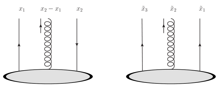
Figure 1: Notations for the momentum fractions in Ref. Hatta:2012cs (left) and in Ref. Braun:2009mi (right).

Note that the total (quark plus gluon) genuine twist-three OAM distribution integrates to zero

$$\int_{0}^{1}dx(L_{3q}(x)+L_{3g}(x))=0.$$ (11)

We can write this as

$$\int_{0}^{1}dxL_{3g}(x)\equiv L_{\mathrm{pot}}=-\int_{0}^{1}dxL_{3q}(x).$$ (12)

The quantity $L_{\mathrm{pot}}$, sometimes called the potential angular momentum Wakamatsu:2010qj , represents the difference between the kinetic (Ji) OAM Ji:1996ek and the canonical (Jaffe-Manohar) OAM Jaffe:1989jz

$$L_{\mathrm{Ji}}^{q}-L_{\mathrm{JM}}^{q}=L_{\mathrm{pot}}.$$ (13)

Roughly speaking, it arises from the difference between the covariant derivative (kinetic momentum) $\vec{x}\times\vec{D}$ and the partial derivative (canonical momentum) $\vec{x}\times\vec{\partial}$ in the definition of OAM. The value of $L_{\mathrm{pot}}$ for an electron in QED has been the subject of debate in the literature Burkardt:2008ua ; Liu:2014fxa ; Ji:2015sio . More recently, $L_{\mathrm{pot}}$ has been calculated in lattice QCD and found to be nonzero Engelhardt:2017miy ; Engelhardt:2019lyy .

Let us now consider the evolution of $L_{q,g}(x)$. Taking the $n$-th moments $L_{q,g}^{n}=\int_{0}^{1}dxx^{n-1}L_{q,g}(x)$, etc., we find

$$L_{q}^{n} = \frac{1}{n+1}(\Sigma^{n+1}+E_{q}^{n+1})-\frac{1}{n+1}\Delta\Sigma^{n}+L^{n}_{3q},$$

$$L_{g}^{n} = \frac{1}{n+1}(G^{n+1}+E_{g}^{n+1})-\frac{2}{n+1}\Delta G^{n}+L^{n}_{3g}\,,$$ (14)

where $L_{3q}$ and $L_{3g}$ are the contributions from the genuine twist three part. The evolution of $\Sigma^{n},G^{n},\Delta\Sigma^{n}$ and $\Delta G^{n}$ in the renormalization scale $\mu^{2}$ is governed by the standard DGLAP anomalous dimensions $\gamma^{n}$ and $\Delta\gamma^{n}$. Moreover, the anomalous dimensions of $E^{n}_{q},E^{n}_{g}$ are the same as those for $\Sigma^{n},G^{n}$. Therefore, if one restricts oneself to the WW part, one can immediately write down the evolution equation

$$\frac{\partial}{\partial t}\begin{pmatrix}L^{n}_{q}\\ L_{g}^{n}\end{pmatrix}^{WW} = \frac{1}{n+1}\begin{pmatrix}\gamma^{n+1}_{qq}&\gamma^{n+1}_{qg}\\ \gamma^{n+1}_{gq}&\gamma^{n+1}_{gg}\end{pmatrix}\begin{pmatrix}\Sigma^{n+1}+E_{q}^{n+1}\\ G^{n+1}+E_{g}^{n+1}\end{pmatrix}-\frac{1}{n+1}\begin{pmatrix}\Delta\gamma^{n}_{qq}&\Delta\gamma^{n}_{qg}\\ 2\Delta\gamma^{n}_{gq}&2\Delta\gamma^{n}_{gg}\end{pmatrix}\begin{pmatrix}\Delta\Sigma^{n}\\ \Delta G^{n}\end{pmatrix}$$ (15)

$$= \begin{pmatrix}\gamma^{n+1}_{qq}&\gamma^{n+1}_{qg}\\ \gamma^{n+1}_{gq}&\gamma^{n+1}_{gg}\end{pmatrix}\begin{pmatrix}L^{n}_{q}\\ L_{g}^{n}\end{pmatrix}^{WW}+\frac{1}{n+1}\begin{pmatrix}\gamma_{qq}^{n+1}-\Delta\gamma^{n}_{qq}&2\gamma_{qg}^{n+1}-\Delta\gamma^{n}_{qg}\\ \gamma_{gq}^{n+1}-2\Delta\gamma^{n}_{gq}&2\gamma_{gg}^{n+1}-2\Delta\gamma^{n}_{gg}\end{pmatrix}\begin{pmatrix}\Delta\Sigma^{n}\\ \Delta G^{n}\end{pmatrix}\,,$$

where

$$t=-\frac{2}{b_{0}}\ln\frac{\alpha_{s}(\mu^{2})}{\alpha_{s}(\mu_{0}^{2})},$$ (16)

with $\alpha_{s}(\mu^{2})=\frac{4\pi}{b_{0}\ln(\mu^{2}/\Lambda_{QCD}^{2})}$ and $b_{0}=\frac{11N_{c}}{3}-\frac{2n_{f}}{3}$. In the WW approximation, (15) holds to all orders in perturbation theory Boussarie:2019icw . To one-loop order, it agrees with the result obtained in Harindranath:1998ve ; Hagler:1998kg , see also, Hoodbhoy:1998yb .

Inclusion of the genuine twist-three parts makes things considerably more complicated. One might naively expect that the genuine twist-three part would evolve with its own anomalous dimensions

$$\frac{\partial}{\partial t}\begin{pmatrix}L^{n}_{3q}\\ L_{3g}^{n}\end{pmatrix}\stackrel{{\scriptstyle?}}{{=}}\begin{pmatrix}A_{n}&B_{n}\\ C_{n}&D_{n}\end{pmatrix}\begin{pmatrix}L_{3q}^{n}\\ L_{3g}^{n}\end{pmatrix}\,,$$ (17)

and therefore the evolution of the full OAMs would be given by

$$\frac{\partial}{\partial t}\begin{pmatrix}L^{n}_{q}\\ L_{g}^{n}\end{pmatrix} \stackrel{{\scriptstyle?}}{{=}} \begin{pmatrix}\gamma^{n+1}_{qq}&\gamma^{n+1}_{qg}\\ \gamma^{n+1}_{gq}&\gamma^{n+1}_{gg}\end{pmatrix}\begin{pmatrix}L^{n}_{q}\\ L_{g}^{n}\end{pmatrix}+\frac{1}{n+1}\begin{pmatrix}\gamma_{qq}^{n+1}-\Delta\gamma^{n}_{qq}&2\gamma_{qg}^{n+1}-\Delta\gamma^{n}_{qg}\\ \gamma_{gq}^{n+1}-2\Delta\gamma^{n}_{gq}&2\gamma_{gg}^{n+1}-2\Delta\gamma^{n}_{gg}\end{pmatrix}\begin{pmatrix}\Delta\Sigma^{n}\\ \Delta G^{n}\end{pmatrix}$$ (18)

$$+\begin{pmatrix}A_{n}-\gamma_{qq}^{n+1}&B_{n}-\gamma_{qg}^{n+1}\\ C_{n}-\gamma_{gq}^{n+1}&D_{n}-\gamma^{n+1}_{gg}\end{pmatrix}\begin{pmatrix}L_{3q}^{n}\\ L_{3g}^{n}\end{pmatrix}\,.$$

However, we shall demonstrate later that this is not the case. In general, different moments (different $n$’s) mix under evolution so that the right hand side of (17) should involve a summation over all moments. This suggests that it is more convenient to study the evolution directly in the $x$-space.

III Evolution of the genuine-twist three part

At first sight, the $\mu^{2}$-evolution of $\Phi_{F}(x_{1},x_{2})$ etc., hence that of $L_{3q,3g}(x)$ seems a challenging open question. However, it is actually known in the context of transverse single spin asymmetry (SSA). There, exactly the same set of operators as in (6)-(9) appear. The difference is that in the case of SSA, one takes the forward matrix element (i.e., $\Delta=0$) in the transversely polarized nucleon state $S^{\mu}=\delta^{\mu}_{i}S_{i}$. The resulting distribution, the Efremov-Teryaev-Qiu-Sterman (ETQS) function Efremov:1984ip ; Qiu:1991wg has been extensively discussed in the literature. Because the evolution is intrinsic to the operators involved, not to external states, and here we only consider the $\Delta\to 0$ limit of the nonforward matrix element, the same evolution equation should apply. The complete derivation of the evolution equation has been given in Braun:2009mi following earlier attempts Kang:2008ey ; Vogelsang:2009pj (see also Schafer:2012ra ; Ma:2012xn ; Yoshida:2016tfh ). The result is too lengthy to be reproduced here, but fortunately, a C++ code is publicly available Pirnay:2013fra . We shall heavily rely on this code in the following.

For this purpose, first we need to clarify the difference in notations between ours and in Braun:2009mi ; Pirnay:2013fra . There the authors introduced the following distributions with three arguments

$$T_{\bar{q}Fq}(\tilde{x}_{1},\tilde{x}_{2},\tilde{x}_{3}),\qquad\Delta T_{\bar{q}Fq}(\tilde{x}_{1},\tilde{x}_{2},\tilde{x}_{3}),\quad T_{3F}^{+}(\tilde{x}_{1},\tilde{x}_{2},\tilde{x}_{3}),\quad\Delta T_{3F}^{+}(\tilde{x}_{1},\tilde{x}_{2},\tilde{x}_{3})\,.$$ (19)

To avoid confusion, we have added a tilde on momentum fractions. Their meaning is self-explanatory from Fig. 1 (beware of the direction of arrows) with the correspondence

$$x_{1}=\tilde{x}_{3},\quad x_{2}-x_{1}=\tilde{x}_{2},\quad x_{2}=-\tilde{x}_{1},\qquad\tilde{x}_{1}+\tilde{x}_{2}+\tilde{x}_{3}=0\,.$$ (20)

The four distributions in (19) are direct analogs of (6)-(9). The plus sign on $T_{3F}$ and $\Delta T_{3F}$ means the contraction of color indices with the $f$-symbol, cf., the comment below (9). We have carefully checked the relative normalization and found the correspondence

$$\Phi_{F}(x_{1},x_{2})\leftrightarrow 2T_{\bar{q}Fq}(-x_{2},x_{2}-x_{1},x_{1}),$$ (21)

$$\widetilde{\Phi}_{F}(x_{1},x_{2})\leftrightarrow-2\Delta T_{\bar{q}Fq}(-x_{2},x_{2}-x_{1},x_{1}),$$ (22)

$$M_{F}(x_{1},x_{2})\leftrightarrow T^{+}_{3F}(-x_{2},x_{2}-x_{1},x_{1}),$$ (23)

$$\widetilde{M}_{F}(x_{1},x_{2})\leftrightarrow-\Delta T^{+}_{3F}(\tilde{x}_{1},\tilde{x}_{2},\tilde{x}_{3})\,.$$ (24)

As observed in Braun:2009mi , $\Delta T^{+}_{3F}$ is not an independent function (see Eq. (32) there). Accordingly, $\widetilde{M}_{F}$ can be eliminated via the corresponding formula

$$\widetilde{M}_{F}(x_{1},x_{2})=-M_{F}(x_{2}-x_{1},x_{2})+M_{F}(x_{1},x_{1}-x_{2}).$$ (25)

This was not noticed in Hatta:2012cs , but it can be indeed derived from the formulas in this reference.

Another complication is that in Ref. Braun:2009mi , the evolution equation has been presented in terms of

$$\mathfrak{S}^{\pm}(\tilde{x}_{1},\tilde{x}_{2},\tilde{x}_{3}),\qquad\mathfrak{F}^{\pm}(\tilde{x}_{1},\tilde{x}_{2},\tilde{x}_{3})$$ (26)

which are particular linear combinations of the distributions in (19). The signs $\pm$ refer to $C$-parity, and the point is that the evolution equation does not mix the $C$-even and $C$-odd functions. From (21)-(24), we find the correspondence

$$2\mathfrak{S}^{+}(\tilde{x}_{1},\tilde{x}_{2},\tilde{x}_{3}) \leftrightarrow \Phi_{F}(x_{1},x_{2})-\Phi_{F}(-x_{1},-x_{2})+\widetilde{\Phi}_{F}(x_{1},x_{2})-\widetilde{\Phi}_{F}(-x_{1},-x_{2})$$ (27)

$$\equiv 2S^{+}(x_{1},x_{2})\,.$$

$$\mathfrak{F}^{+}(\tilde{x}_{1},\tilde{x}_{2},\tilde{x}_{3}) \leftrightarrow M_{F}(x_{1},x_{2})+\widetilde{M}_{F}(x_{1},x_{2})$$ (28)

$$\equiv F^{+}(x_{1},x_{2})\,.$$

The distributions $\mathfrak{S}^{+}$ and $\mathfrak{F}^{+}$ have the following symmetry Braun:2009mi

$$\mathfrak{S}^{+}(-\tilde{x})=\mathfrak{S}^{+}(\tilde{x}),\qquad\mathfrak{F}^{+}(-\tilde{x})=-\mathfrak{F}^{+}(\tilde{x}).$$ (29)

In our case, we find from (10)

$$S^{+}(-x_{1},-x_{2})=-S^{+}(x_{1},x_{2}),\qquad F^{+}(-x_{1},-x_{2})=F(x_{1},x_{2}).$$ (31)

Notice the differences in sign, which is simply due to the fact that we are dealing with different matrix elements (longitudinally polarized nucleon, finite momentum transfer). This however causes no problem in practice because the evolution equation automatically preserves the symmetry property of the initial conditions.

Note also that in (27) and (28), we only showed the $C$-even distributions. This is because the OAM distributions are $C$-even ($PT$-even) Hatta:2011ku . Indeed, the twist-three part of (4) and (5) can be solely written in terms of $C$-even functions $S^{+}$ and $F^{+}$. It is not difficult to show that

$$L_{3q}(x) = -2x\int^{1}_{x}dx_{1}\int_{-1}^{1}dx_{2}S^{+}(x_{1},x_{2})\frac{1}{x_{1}^{2}(x_{1}-x_{2})}$$ (32)

$$-2x\int^{1}_{x}dx_{1}\int_{-1}^{1}dx_{2}(S^{+}(x_{1},x_{2})-S^{+}(x_{2},x_{1})){\cal P}\frac{1}{x_{1}(x_{1}-x_{2})^{2}}\,.$$

In the gluon case, let us write

$$L_{3g}(x) = L_{3g,S}(x)+L_{3g,F}(x),$$ (33)

where

$$L_{3g,S}(x) = 4x\int^{1}_{x}\frac{dx^{\prime}}{x^{\prime 3}}\int dXS^{+}(x_{1},x_{2})$$ (34)

$$L_{3g,F}(x) = 2x\int^{1}_{x}dx_{1}\int^{1}_{-1}dx_{2}(F^{+}(x_{1},x_{2})-F^{+}(x_{2},x_{1})){\cal P}\frac{1}{x_{1}^{2}(x_{1}-x_{2})^{2}}$$ (35)

$$+4x\int^{1}_{x}dx_{1}\int^{1}_{-1}dx_{2}F^{+}(x_{1},x_{2}){\cal P}\frac{1}{x_{1}^{3}(x_{1}-x_{2})}\,.$$

In terms of moments, we have

$$L_{3q}^{n}=-\frac{2}{n+1}\int_{0}^{1}dx_{1}\int_{-1}^{1}dx_{2}\Biggl{[}S^{+}(x_{1},x_{2})\frac{x_{1}^{n-1}}{x_{1}-x_{2}}+(S^{+}(x_{1},x_{2})-S^{+}(x_{2},x_{1})){\cal P}\frac{x_{1}^{n}}{(x_{1}-x_{2})^{2}}\Biggr{]}\,.$$ (36)

$$L_{3g}^{n} = \frac{4}{n+1}\int_{0}^{1}dx\int_{-1}^{1}dXx^{n-2}S^{+}\left(X+\frac{x}{2},X-\frac{x}{2}\right)$$ (37)

$$-\frac{2}{n+1}\int_{0}^{1}dx_{1}\int_{-1}^{1}dx_{2}\Biggl{[}(F^{+}(x_{1},x_{2})-F^{+}(x_{2},x_{1})){\cal P}\frac{x_{1}^{n-1}}{(x_{1}-x_{2})^{2}}+2F^{+}(x_{1},x_{2}){\cal P}\frac{x_{1}^{n-2}}{(x_{1}-x_{2})}\Biggr{]}\,.$$

Eqs. (32)-(37) are the starting point of our numerical analysis which we now turn to.

IV Numerical results

In this section, we present the one-loop scale evolution of the genuine twist-three part of the OAM distributions $L_{3q,3g}(x,\mu)$. Our numerical results are based on a C++ code developed by Pirnay Pirnay:2013fra . Although the code is intended for the ETQS function, it can be straightforwardly adapted to the present problem with almost no change. The only thing one should keep in mind is that the symmetry properties of the various distributions are different, see (29) and (30). However, this does not cause extra complications since the evolution equation preserves this symmetry, and one just needs to properly implement the relevant symmetry in the initial conditions.

We set the number of lattice sites in the interval $-1\leq x\leq 1$ to be $N_{x}=2001$ (this has to be an odd number in the code), so that the lattice size is $\Delta x=0.001$. As for the initial conditions, currently nothing is known about the functional forms of the genuine twist-three distributions $\Phi(x_{1},x_{2})$, etc., except that they must vanish at kinematic boundaries (e.g., $x_{1}=\pm 1$) and obey the symmetry properties (10). We thus introduce three different models at the initial scale $\mu_{0}^{2}$

$$\Phi_{F}(x_{1},x_{2}) = \begin{cases}0,&|x_{1}|\geq 1\parallel|x_{2}|\geq 1\parallel|x_{2}-x_{1}|\geq 1\\ 2(x_{1}-x_{2})f(x_{1},x_{2}),&\mathrm{otherwise}\end{cases}$$ (38)

$$\widetilde{\Phi}_{F}(x_{1},x_{2}) = \begin{cases}0,&|x_{1}|\geq 1\parallel|x_{2}|\geq 1\parallel|x_{2}-x_{1}|\geq 1\\ 2f(x_{1},x_{2}),&\mathrm{otherwise}\end{cases}$$ (39)

$$M_{F}(x_{1},x_{2}) = \begin{cases}0,&|x_{1}|\geq 1\parallel|x_{2}|\geq 1\parallel|x_{2}-x_{1}|\geq 1\\ (x_{1}^{2}-x_{2}^{2})f(x_{1},x_{2}),&\mathrm{otherwise}\end{cases}$$ (40)

with

1. $f(x_{1},x_{2})=\frac{1}{10}(1-x_{1}^{2})(1-x_{2}^{2})(1-(x_{1}-x_{2})^{2})$ ;

2. $f(x_{1},x_{2})=x_{1}x_{2}(1-x_{1}^{2})(1-x_{2}^{2})(1-(x_{1}-x_{2})^{2})$ ;

3. $f(x_{1},x_{2})=x^{2}_{1}x^{2}_{2}(1-x_{1}^{2})(1-x_{2}^{2})(1-(x_{1}-x_{2})^{2})$ .

The overall sign has been fixed such that the potential angular momentum (12) calculated from these initial conditions is positive $L_{\mathrm{pot}}>0$, as suggested by an intuitive argument Burkardt:2012sd as well as a recent lattice calculation Engelhardt:2017miy . We then use (27) and (28) to convert the above initial conditions into those of $S^{+}$ and $F^{+}$. They are further converted into $\mathfrak{S}^{+}(\tilde{x}_{1},\tilde{x}_{2},\tilde{x}_{3})=S^{+}(x_{1},x_{2})$ and $\mathfrak{F}^{+}(\tilde{x}_{1},\tilde{x}_{2},\tilde{x}_{3})=F^{+}(x_{1},x_{2})$ since the code requires $\mathfrak{S}^{+}$ and $\mathfrak{F}^{+}$ as the initial conditions. In the end of the numerical calculation, we convert the final results of $\mathfrak{S}^{+}$ and $\mathfrak{F}^{+}$ back into $S^{+}$ and $F^{+}$. Finally, we compute the twist-three OAM distributions $L_{3q}(x)$ and $L_{3g}(x)$, Eqs. (32)-(35), numerically by using the Simpson’s rule. The integrands of $L_{3q}(x)$ and $L_{3g}(x)$ may have singularities when $x_{1}\to 0$ or $x^{\prime}\to 0$. Such singularities may be present already in the initial conditions, or can be dynamically generated by the evolution (see below). To improve the numerical accuracy when this happens, we first fit the integrand $f(x_{1})$ (or $f(x^{\prime})$) in the small-$x$ region (in practice, $x<0.005$) by the power function $ax_{1}^{b}$ (or $ax^{\prime b}$) with $b<0$. Then we split as

$$\int_{x}^{1}dx_{1}f(x_{1})=\int_{x}^{1}dx_{1}(f(x_{1})-ax_{1}^{b})+\int_{x}^{1}dx_{1}ax_{1}^{b}.$$ (41)

The integrand of the first term has no singularities so the integral can be evaluated accurately. The second integral can be done analytically.

As a warm-up, let us first check the sum rules Hatta:2012cs :

$$\int_{0}^{1}dxL_{3g,F}(x) = 0,$$ (42)

$$\int_{0}^{1}dx(L_{3q}(x)+L_{3g,S}(x)) = 0\,.$$ (43)

This is a more detailed version of (11) (see (33)). We numerically evolve each of the initial conditions from $\mu_{0}^{2}=1$ GeV² to $\mu^{2}=10$ GeV². The numerical results of the left-handed-sides of (42) and (43) for the three different initial conditions are shown in Table 1. As a reference, we also show the value of the potential angular momentum $L_{\mathrm{pot}}$ (12) in these models. We see that the sum rules are satisfied up to numerical errors.

Table 1: Numerical results of the sum rules.

	Initial condition 1	Initial condition 2	Initial condition 3
$\int_{0}^{1}dxL_{3g,F}(x)$ at $\mu_{0}^{2}=1$ GeV2	$0.0006$	$0.0006$	$0.0002$
$\int_{0}^{1}dxL_{3g,F}(x)$ at $\mu^{2}=10$ GeV2	-0.00007	0.0004	0.00016
$\int_{0}^{1}dx(L_{3q}(x)+L_{3g,S}(x))$ at $\mu_{0}^{2}=1$ GeV2	$4\times 10^{-7}$	-0.0006	-0.0002
$\int_{0}^{1}dx(L_{3q}(x)+L_{3g,S}(x))$ at $\mu^{2}=10$ GeV2	0.00014	-0.0007	-0.0002
$L_{\mathrm{pot}}$ at $\mu_{0}^{2}=1$ GeV2	0.234	0.185	0.069
$L_{\mathrm{pot}}$ at $\mu^{2}=10$ GeV2	0.162	0.077	0.032

Next, we study whether the moments of the twist-three OAM distributions $L^{n}_{3q}$ (flavor singlet) and $L^{n}_{3g}$ satisfy the homogeneous equation (17). This can be tested by assuming (17) and considering an infinitesimal evolution

$$\begin{pmatrix}L^{n}_{3q}\\ L_{3g}^{n}\end{pmatrix}_{\mu^{2}}\approx\begin{pmatrix}L^{n}_{3q}\\ L_{3g}^{n}\end{pmatrix}_{\mu_{0}^{2}}+\frac{2}{b_{0}}\ln\frac{\alpha_{s}(\mu^{2}_{0})}{\alpha_{s}(\mu^{2})}\begin{pmatrix}A_{n}&B_{n}\\ C_{n}&D_{n}\end{pmatrix}\begin{pmatrix}L^{n}_{3q}\\ L_{3g}^{n}\end{pmatrix}_{\mu^{2}_{0}}\,.$$ (44)

In practice, we use $\mu_{0}^{2}=1$ GeV² and $\mu^{2}=1.01$ GeV². This means that $n_{f}=3$, and the code uses the value $\Lambda_{QCD}=0.204$ GeV in this case. In order to extract $A_{n},B_{n},...$, it is not enough to consider one initial condition since (44) contains two equations but there are four unknowns. But we can combine any two sets of initial conditions and form a solvable system of linear equations. We will label the results of $A_{n},B_{n},...$ obtained from the $i$-th and $j$-th initial conditions as $A_{n}(ij),B_{n}(ij)$,… and compare these with the known anomalous dimensions of the twist-two operators

$$\begin{pmatrix}\gamma^{n+1}_{qq}&\gamma^{n+1}_{qg}\\ \gamma^{n+1}_{gq}&\gamma^{n+1}_{gg}\end{pmatrix}=\begin{pmatrix}\frac{4}{3}\left[-\frac{1}{2}+\frac{1}{(n+1)(n+2)}-2\sum_{k=2}^{n+1}\frac{1}{k}\right]&n^{\prime}_{f}\frac{n^{2}+3n+4}{(n+1)(n+2)(n+3)}\\ \frac{4}{3}\frac{n^{2}+3n+4}{(n+1)n(n+2)}&6\left[-\frac{1}{12}+\frac{1}{n(n+1)}+\frac{1}{(n+2)(n+3)}-\sum_{k=2}^{n+1}\frac{1}{k}\right]-\frac{n^{\prime}_{f}}{3}\end{pmatrix}\,.$$ (45)

We make this comparison in the (naive) hope that there may be a significant cancelation in the second line of (18) so that the evolution equation for the total OAM distributions is formally the same as that in the WW approximation. Note that we set $n^{\prime}_{f}=2$ in (45) because this is the value used in the one-loop evolution kernel in the code. It is different from $n_{f}$ used in the running coupling constant. The latter depends on the scale $\mu^{2}$.

The comparison results are shown in Fig. 2. The numerically extracted $A_{n}$, $B_{n}$, $C_{n}$ and $D_{n}$ of the twist-three operators are not universal because they depend on the choice of the initial condition. This implies that (17) is not valid and the moments of different $n$’s will mix with each other during the evolution. Interestingly, however, we find that the large-$n$ behaviors of the $A_{n}$, $B_{n}$, $C_{n}$ and $D_{n}$ are given by

$$A_{n} = -\frac{N_{c}^{2}-1}{N_{c}}\ln{n}+\mathrm{const.}$$ (46)

$$B_{n} = \mathrm{const.}$$

$$C_{n} = \mathrm{const.}$$

$$D_{n} = -2N_{c}\ln{n}+\mathrm{const.}\,,$$

which agree with the $n$-dependence of $\gamma^{n+1}$’s when $n$ is large. The constant terms in the $A_{n}$, $B_{n}$, $C_{n}$ and $D_{n}$ are not universal and depend on the choice of the initial conditions. The leading, logarithmic terms are called the cusp anomalous dimensions. We have thus found that, when $n$ is large, (17) is approximately valid and the second line of (18) is small. This means that when $x\sim 1$, the total OAM distribution approximately satisfies the same evolution equation as in the WW approximation. We note that the emergence of the cusp anomalous dimension in the twist-three distributions in the large-$x$ limit was pointed out in Braun:2009mi in a different context. Incidentally, we found the correct asymptotic behavior (46) only after fixing a typo in the code mentioned in Footnote 5 (the factor of $N_{c}$).

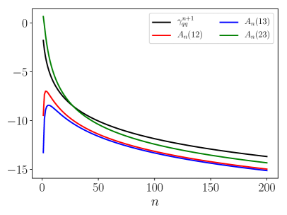
(a) $A_{n}$’s and $\gamma^{n+1}_{qq}$.

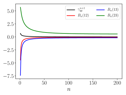
(b) $B_{n}$’s and $\gamma^{n+1}_{qg}$.

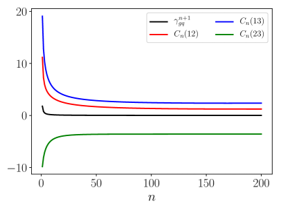
(c) $C_{n}$’s and $\gamma^{n+1}_{gq}$.

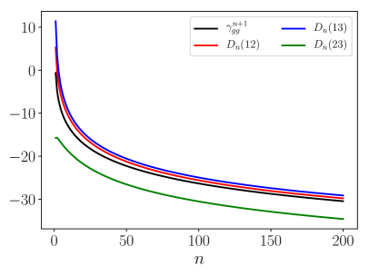
(d) $D_{n}$’s and $\gamma^{n+1}_{gg}$.

Figure 2: Comparison between the numerically extracted $A_{n}$, $B_{n}$, $C_{n}$ and $D_{n}$ and the anomalous dimensions of the twist-two operators.

We then study the evolution from $\mu_{0}^{2}=1$ GeV² to $\mu^{2}=10$ GeV². The initial and final twist-three OAM distributions are plotted in Fig. 3. We note that both $L_{3q}(x)$ (flavor singlet) and $L_{3g}(x)$ develop singular behaviors at small-$x$ during the evolution, even though their initial conditions are regular at $x=0$. We fit the singular behavior by the power function $ax^{b}$ with $b<0$ and find that $b$ depends on the choice of initial conditions. But it always satisfies $b>-1$ in our three sets of initial conditions, which guarantees that both $L_{3q}(x)$ and $L_{3g}(x)$ are integrable in the range $0\leq x\leq 1$. The situation is somewhat similar to the DGLAP evolution of the WW part Hatta:2018itc , where a singularity is developed from nonsingular initial conditions. In that case it was possible to gain some analytical insights, but in the present case a similar analytical study is difficult due to the complexity of the twist-three evolution. We also note that, curiously, the three-gluon part $L_{3g,F}(x)$ of $L_{3g}(x)$, see (33), evolves very weakly with the renormalization scale. Since this part does not contribute to the integrated OAM (42), we suspect that in general it plays a minor role in the nucleon spin decomposition. We however note that only for the initial condition 1, $L_{3g,F}(x)$ shows a sharp drop in the smallest $x$ bins that can be fitted by a power law as shown in Fig. 4. In fact, such a rapid behavior is necessary to satisfy the sum rule in this case.

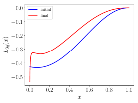
(a) $L_{3q}(x)$ from initial condition 1.

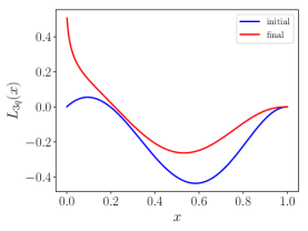
(b) $L_{3q}(x)$ from initial condition 2.

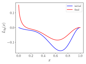
(c) $L_{3q}(x)$ from initial condition 3.

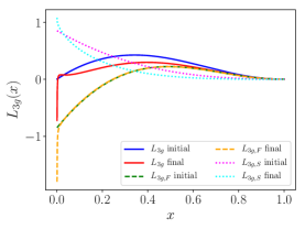
(d) $L_{3g}(x)$ from initial condition 1.

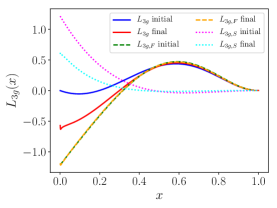
(e) $L_{3g}(x)$ from initial condition 2.

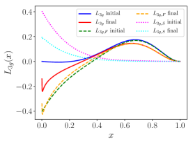
(f) $L_{3g}(x)$ from initial condition 3.

Figure 3: Evolution of $L_{3q}(x)$ and $L_{3g}(x)$ from the initial $\mu_{0}^{2}=1$ GeV² to the final $\mu^{2}=10$ GeV² scales for three different initial conditions.

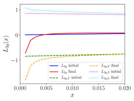
Figure 4: Fig. 3(d), zoomed in on the small-$x$ region.

Finally we study the $\mu^{2}$-dependence of the potential angular momentum (12). Here we are also interested in the flavor nonsinglet part $L_{\mathrm{pot}}^{u-d}$ because the recent lattice calculations have shown that this quantity is positive and large Engelhardt:2017miy ; Engelhardt:2019lyy . In fact, the singlet part $L^{u+d}_{\mathrm{pot}}$ is numerically much smaller due to a large cancelation between the $u$- and $d$-quark contributions. We have not mentioned the evolution in the flavor nonsinglet sector so far, but of course it is simpler than the singlet case because there is no mixing with the three-gluon part. The code can handle this as well.

We evolve the initial conditions 2 and 3 from $\mu_{0}^{2}=2$ GeV² to $\mu^{2}=12$ GeV² and compute how $L_{\mathrm{pot}}$ changes with the scale for both the flavor singlet and nonsinglet parts. The initial and final scales are chosen such that the number of dynamical quarks $n_{f}$ in the running coupling does not change in the course of evolution. The results are shown in the left panel of Fig. 5. In both cases, the evolution tends to suppress the magnitude of $L_{\mathrm{pot}}$, with a stronger suppression in the singlet case. This can be understood as arising from the mixing with the three-gluon correlator. We have fitted these results in the form

$$L_{\mathrm{pot}}(\mu^{2})=L_{\mathrm{pot}}(\mu_{0}^{2})\bigg{(}\frac{\ln{\mu_{0}^{2}/\Lambda^{2}_{QCD}}}{\ln{\mu^{2}/\Lambda^{2}_{QCD}}}\bigg{)}^{\gamma}\,,$$ (47)

which features an ‘anomalous dimension’ $\gamma$. Here $\Lambda_{QCD}=0.175$ GeV is used in the code for $n_{f}=4$. We find that $\gamma$ is $\mu$-dependent as shown in the right panel of Fig. 5. It also depends on the initial condition. This means that the evolution of $L_{\mathrm{pot}}$ cannot be characterized by a single anomalous dimension even in the nonsinglet sector due to the mixing between different moments. From the obtained behavior of $\gamma$, we deduce that $L_{\mathrm{pot}}\to 0$ as $\mu\to\infty$ (though this has to be checked more carefully). Therefore, the asymptotic result for the integrated OAM

$$L_{q}(\mu\to\infty)\approx-\frac{1}{2}\Delta\Sigma+\frac{1}{2}\frac{3n_{f}}{16+3n_{f}},\qquad L_{g}(\mu\to\infty)\approx-\Delta G(\mu)+\frac{1}{2}\frac{16}{16+3n_{f}},$$ (48)

obtained in the WW approximation Ji:1995cu will not be affected. The subleading corrections to (48) have the $\mu$-dependence of the form (47) with $\gamma=\frac{2(16+3n_{f})}{9b_{0}}\approx 0.75$ (for $n_{f}=4$) Ji:1995cu . Since this is smaller than the value shown in Fig. 5, it seems that $L_{\mathrm{pot}}$ can be neglected in the large-$\mu$ region.

In Ji:2015sio , it has been shown that $L_{\mathrm{pot}}$ vanishes for a single electron state to one-loop order in QED. This is not necessarily in contradiction to the present result. The operator $\vec{x}\times\bar{\psi}\gamma^{+}\vec{A}\psi$ (in the light-cone gauge) relevant to $L_{\mathrm{pot}}$ mixes with a tower of operators $\vec{x}\times\bar{\psi}\gamma^{+}D^{\mu}D^{\nu}\cdots\vec{A}\psi$ and if these higher moments have nonvanishing initial values (as in our initial conditions), they will affect the renormalization of $L_{\mathrm{pot}}$.

(a) Scale dependence of $L_{\mathrm{pot}}$.

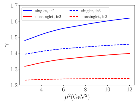
(b) Scale dependence of $\gamma$ in (47).

Figure 5: Evolution of $L_{\mathrm{pot}}$ for initial conditions 2 and 3.

V Conclusions

In this paper, we have studied, for the first time, the one-loop QCD evolution of the genuine twist-three part of the OAM distributions. In particular, the scale variation of the potential angular momentum has been demonstrated. As anticipated by the complicated relations between $L_{3q,3g}(x)$ and the underlying distributions $S^{+}$ and $F^{+}$ (see, e.g., (32)), different moments of $L_{3q,3g}(x)$ mix under evolution except in the large-$n$ limit. This suggests that it is more convenient to look at the evolution directly in the $x$-space. Together with the known evolution of the WW part, the one-loop evolution of the total OAM distributions $L_{q,g}(x)$ is now fully under control and ready for phenomenological applications.

In the present C++ code, the grid in $x$ is uniform and the smallest value of $x$ that we achieved is 0.001. It is not realistic to go to much lower values of $x$ because it is computationally too expensive. In view of the recent controversy regarding the small-$x$ asymptotic behavior of the OAM distributions Hatta:2018itc ; Kovchegov:2019rrz ; Boussarie:2019icw , it would be interesting to modify the code (e.g., set up a grid in $\ln 1/x$ instead of $x$) to zoom in on to the small-$x$ region as was done for the WW part Hatta:2018itc . We leave this to future work.

References

- (1) A. Adare et al. [PHENIX Collaboration], Phys. Rev. Lett. 103, 012003 (2009) [arXiv:0810.0694 [hep-ex]].
- (2) A. Airapetian et al. [HERMES Collaboration], JHEP 1008, 130 (2010) [arXiv:1002.3921 [hep-ex]].
- (3) L. Adamczyk et al. [STAR Collaboration], Phys. Rev. D 86, 032006 (2012) [arXiv:1205.2735 [nucl-ex]].
- (4) M. G. Alekseev et al. [COMPASS Collaboration], Phys. Lett. B 693, 227 (2010) [arXiv:1007.4061 [hep-ex]].
- (5) L. Adamczyk et al. [STAR Collaboration], Phys. Rev. Lett. 115, no. 9, 092002 (2015) [arXiv:1405.5134 [hep-ex]].
- (6) Y. Prok et al. [CLAS Collaboration], Phys. Rev. C 90, no. 2, 025212 (2014) [arXiv:1404.6231 [nucl-ex]].
- (7) D. de Florian, R. Sassot, M. Stratmann and W. Vogelsang, Phys. Rev. Lett. 113, no. 1, 012001 (2014) [arXiv:1404.4293 [hep-ph]].
- (8) E. R. Nocera et al. [NNPDF Collaboration], Nucl. Phys. B 887, 276 (2014) [arXiv:1406.5539 [hep-ph]].
- (9) N. Sato et al. [Jefferson Lab Angular Momentum Collaboration], Phys. Rev. D 93, no. 7, 074005 (2016) [arXiv:1601.07782 [hep-ph]].
- (10) R. L. Jaffe and A. Manohar, Nucl. Phys. B 337, 509 (1990).
- (11) J. Adam et al. [STAR Collaboration], arXiv:1906.02740 [hep-ex].
- (12) A. Accardi et al., Eur. Phys. J. A 52, no. 9, 268 (2016) [arXiv:1212.1701 [nucl-ex]].
- (13) Y. Hatta and S. Yoshida, JHEP 1210, 080 (2012) [arXiv:1207.5332 [hep-ph]].
- (14) C. Lorce and B. Pasquini, Phys. Rev. D 84, 014015 (2011) [arXiv:1106.0139 [hep-ph]].
- (15) Y. Hatta, Phys. Lett. B 708, 186 (2012) [arXiv:1111.3547 [hep-ph]].
- (16) C. Lorce, B. Pasquini, X. Xiong and F. Yuan, Phys. Rev. D 85, 114006 (2012) [arXiv:1111.4827 [hep-ph]].
- (17) A. Harindranath and R. Kundu, Phys. Rev. D 59, 116013 (1999) [hep-ph/9802406].
- (18) P. Hagler and A. Schafer, Phys. Lett. B 430, 179 (1998) [hep-ph/9802362].
- (19) A. Courtoy, G. R. Goldstein, J. O. Gonzalez Hernandez, S. Liuti and A. Rajan, Phys. Lett. B 731, 141 (2014) [arXiv:1310.5157 [hep-ph]].
- (20) X. Ji, F. Yuan and Y. Zhao, Phys. Rev. Lett. 118, no. 19, 192004 (2017) [arXiv:1612.02438 [hep-ph]].
- (21) Y. Hatta, Y. Nakagawa, F. Yuan, Y. Zhao and B. Xiao, Phys. Rev. D 95, no. 11, 114032 (2017) [arXiv:1612.02445 [hep-ph]].
- (22) S. Bhattacharya, A. Metz and J. Zhou, Phys. Lett. B 771, 396 (2017) [arXiv:1702.04387 [hep-ph]].
- (23) S. Bhattacharya, A. Metz, V. K. Ojha, J. Y. Tsai and J. Zhou, arXiv:1802.10550 [hep-ph].
- (24) P. Hoodbhoy, X. D. Ji and W. Lu, Phys. Rev. D 59, 014013 (1999) [hep-ph/9804337].
- (25) R. Boussarie, Y. Hatta and F. Yuan, arXiv:1904.02693 [hep-ph].
- (26) Y. Hatta and D. J. Yang, Phys. Lett. B 781, 213 (2018) [arXiv:1802.02716 [hep-ph]].
- (27) J. More, A. Mukherjee and S. Nair, Eur. Phys. J. C 78, no. 5, 389 (2018) [arXiv:1709.00943 [hep-ph]].
- (28) Y. V. Kovchegov, JHEP 1903, 174 (2019) [arXiv:1901.07453 [hep-ph]].
- (29) A. V. Efremov and O. V. Teryaev, Phys. Lett. 150B, 383 (1985).
- (30) J. w. Qiu and G. F. Sterman, Nucl. Phys. B 378, 52 (1992).
- (31) V. M. Braun, A. N. Manashov and B. Pirnay, Phys. Rev. D 80, 114002 (2009) Erratum: [Phys. Rev. D 86, 119902 (2012)] [arXiv:0909.3410 [hep-ph]].
- (32) Z. B. Kang and J. W. Qiu, Phys. Rev. D 79, 016003 (2009) [arXiv:0811.3101 [hep-ph]].
- (33) W. Vogelsang and F. Yuan, Phys. Rev. D 79, 094010 (2009) [arXiv:0904.0410 [hep-ph]].
- (34) B. M. Pirnay, arXiv:1307.1272 [hep-ph].
- (35) X. Ji, X. Xiong and F. Yuan, Phys. Rev. D 88, no. 1, 014041 (2013) [arXiv:1207.5221 [hep-ph]].
- (36) M. Wakamatsu, Phys. Rev. D 81, 114010 (2010) [arXiv:1004.0268 [hep-ph]].
- (37) X. D. Ji, Phys. Rev. Lett. 78, 610 (1997) [hep-ph/9603249].
- (38) M. Burkardt and H. BC, Phys. Rev. D 79, 071501 (2009) [arXiv:0812.1605 [hep-ph]].
- (39) T. Liu and B. Q. Ma, Phys. Rev. D 91, 017501 (2015) [arXiv:1412.7775 [hep-ph]].
- (40) X. Ji, A. Schäfer, F. Yuan, J. H. Zhang and Y. Zhao, Phys. Rev. D 93, no. 5, 054013 (2016) [arXiv:1511.08817 [hep-ph]].
- (41) M. Engelhardt, Phys. Rev. D 95, no. 9, 094505 (2017) [arXiv:1701.01536 [hep-lat]].
- (42) M. Engelhardt, J. Green, N. Hasan, S. Krieg, S. Meinel, J. Negele, A. Pochinsky and S. Syritsyn, PoS SPIN 2018, 047 (2019) [arXiv:1901.00843 [hep-lat]].
- (43) A. Schafer and J. Zhou, Phys. Rev. D 85, 117501 (2012) [arXiv:1203.5293 [hep-ph]].
- (44) J. P. Ma and Q. Wang, Phys. Lett. B 715, 157 (2012) [arXiv:1205.0611 [hep-ph]].
- (45) S. Yoshida, Phys. Rev. D 93, no. 5, 054048 (2016) [arXiv:1601.07737 [hep-ph]].
- (46) M. Burkardt, Phys. Rev. D 88, no. 1, 014014 (2013) [arXiv:1205.2916 [hep-ph]].
- (47) X. D. Ji, J. Tang and P. Hoodbhoy, Phys. Rev. Lett. 76, 740 (1996) [hep-ph/9510304].