Learning with Average Precision: Training
Image Retrieval with a Listwise Loss

Abstract

Image retrieval can be formulated as a ranking problem where the goal is to order database images by decreasing similarity to the query. Recent deep models for image retrieval have outperformed traditional methods by leveraging ranking-tailored loss functions, but important theoretical and practical problems remain. First, rather than directly optimizing the global ranking, they minimize an upper-bound on the essential loss, which does not necessarily result in an optimal mean average precision (mAP). Second, these methods require significant engineering efforts to work well, e.g., special pre-training and hard-negative mining. In this paper we propose instead to directly optimize the global mAP by leveraging recent advances in listwise loss formulations. Using a histogram binning approximation, the AP can be differentiated and thus employed to end-to-end learning. Compared to existing losses, the proposed method considers thousands of images simultaneously at each iteration and eliminates the need for ad hoc tricks. It also establishes a new state of the art on many standard retrieval benchmarks. Models and evaluation scripts have been made available at: https://europe.naverlabs.com/Deep-Image-Retrieval/.

1 Introduction

Figure 1: Illustration of the differences between a local ranking loss (here triplet-based) and our listwise loss. The triplet loss (left) performs gradient updates based on a small number of examples, which is not guarranteed to be aligned with a ranking metric. In contrast, the listwise loss (right) considers a large number of images simultaneously and directly optimizes the Average-Precision computed from these images.

Image retrieval consists in finding, given a query, all images containing relevant content within a large database. Relevance here is defined at the instance level and retrieval typically consists in ranking in top positions database images with the same object instance as the one in the query. This important technology serves as a building block for popular applications such as image-based item identification (e.g., fashion items [12, 35, 60] or products [53]) and automatic organization of personal photos [19].

Most instance retrieval approaches rely on computing image signatures that are robust to viewpoint variations and other types of noise. Interestingly, signatures extracted by deep learned models have recently outperformed keypoint-based traditional methods [16, 17, 46]. This good performance was enabled by the ability of deep models to leverage a family of loss functions well-suited to the ranking problem. Compared to classification losses previously used for retrieval with less success [3, 4, 47], ranking-based loss functions directly optimize for the end task, enforcing intra-class discrimination and more fine-grained instance-level image representations [17]. Ranking losses used to date consider either image pairs [45], triplets [17], quadruplets [10], or $n$-tuples [52]. Their common principle is to subsample a small set of images, verify that they locally comply with the ranking objective, perform a small model update if they do not, and repeat these steps until convergence.

Despite their effectiveness, important theoretical and practical problems remain. In particular, it has been shown that these ranking losses are upper bounds on a quantity known as the essential loss [34], which in turn is an upper bound on standard retrieval metrics such as mean average precision (mAP) [33]. Thus, optimizing these ranking losses is not guaranteed to give results that also optimize mAP. Hence there is no theoretical guarantee that these approaches yield good performance in a practical system. Perhaps for this reason, many tricks are required to obtain good results, such as pre-training for classification [1, 17], combining multiple losses [9, 11], and using complex hard-negative mining strategies [14, 20, 37, 38]. These engineering heuristics involve additional hyper-parameters and are notoriously complicated to implement and tune [24, 58].

In this paper, we investigate a new type of ranking loss that remedy these issues altogether by directly optimizing mAP (see Fig. 1). Instead of considering a couple of images at a time, it optimizes the global ranking of thousands of images simultaneously. This practically renders the aforementioned tricks unnecessary while improving the performance at the same time. Specifically, we leverage recent advances in listwise loss functions that allow to reformulate AP using histogram binning [23, 24, 58]. AP is normally non-smooth and not differentiable, and cannot be directly optimized in gradient-based frameworks. Nevertheless, histogram binning (or soft-binning) is differentiable and can be used to replace the non-differentiable sorting operation in the AP, making it amenable to deep learning. He et al. [24] recently presented outstanding results in the context of patch verification, patch retrieval and image matching based on this technique.

In this work, we follow the same path and present an image retrieval approach directly optimized for mAP. To that aim, we train with large batches of high-resolution images that would normally considerably exceed the memory of a GPU. We therefore introduce an optimization scheme that renders training feasible for arbitrary batch sizes, image resolutions and network depths. In summary, we make three main contributions:

• We present, for the first time, an approach to image retrieval leveraging a listwise ranking loss directly optimizing the mAP. It hinges upon a dedicated optimization scheme that handles extremely large batch sizes with arbitrary image resolutions and network depths.

• We demonstrate the many benefits of using our listwise loss in terms of coding effort, training budget and final performance via a ceteris paribus analysis on the loss.

• We outperform the state-of-the-art results for comparable training sets and networks.

The paper is organized as follows: Section 2 discusses related work, Section 3 describes the proposed method, Section 4 present an experimental study, and Section 5 presents our conclusions.

2 Related work

Early works on instance retrieval relied on local patch descriptors (e.g., SIFT [36]), aggregated using bag-of-words representations [13] or more elaborate schemes [15, 18, 55, 29], to obtain image-level signatures that could then be compared to one another in order to find their closest matches. Recently, image signatures extracted with CNNs have emerged as an alternative. While initial work used neuron activations extracted from off-the-shelf networks pre-trained for classification [3, 4, 45, 47, 56], it was later shown that networks could be trained specifically for the task of instance retrieval in an end-to-end manner using a siamese network [17, 46]. The key was to leverage a loss function that optimizes ranking instead of classification. This class of approaches represents the current state of the art in image retrieval with global representations [17, 46].

Image retrieval can indeed be seen as a learning to rank problem [6, 8, 34, 57]. In this framework, the task is to determine in which (partial) order elements from the training set should appear. It is solved using metric learning combined with an appropriate ranking loss. Most works in image retrieval have considered pairwise (e.g., contrastive [45]) or tuplewise (e.g., triplet-based [16, 50], $n$-tuple-based [52]) loss functions, which we call local loss functions because they act on a fixed and limited number of examples before computing the gradient. For such losses, training consists in repeatedly sampling random and difficult pairs or triplets of images, computing the loss, and backpropagating its gradient. However, several works [14, 24, 27, 40, 48] pointed out that properly optimizing a local loss can be a challenging task, for several reasons. First, it requires a number of ad hoc heuristics such as pre-training for classification [1, 17], combining several losses [9, 11] and biasing the sampling of image pairs by mining hard or semi-hard negative examples [14, 20, 37, 38]. Besides being non trivial [21, 51, 59], mining hard examples is often time consuming. Another major problem that has been overlooked so far is the fact that local loss functions only optimize an upper bound on the true ranking loss [34, 58]. As such, there is no theoretical guarantee that the minimum of the loss actually corresponds to the minimum of the true ranking loss.

In this paper, we take a different approach and directly optimize the mean average precision (mAP) metric. While the AP is a non-smooth and non-differentiable function, He et al. [23, 24] have recently shown that it can be approximated based on the differentiable approximation to histogram binning proposed in [58] (and also used in [7]). This approach radically differs from those based on local losses. The use of histogram approximations to mAP is called listwise in [34], as the loss function takes a variable (possibly large) number of examples at the same time and optimizes their ranking jointly. The AP loss introduced by He et al.  [23] is specially tailored to deal with score ties naturally occurring with hamming distances in the context of image hashing. Interestingly, the same formulation is also proved successful for patch matching and retrieval [24]. Yet their tie-aware formulation poses important convergence problems and requires several approximations to be usable in practice. In contrast, we propose a straightforward formulation of the AP loss that is stable and performs better. We apply it to image retrieval, which is a rather different task, as it involves high-resolution images with significant clutter, large viewpoint changes and deeper networks.

Apart from [23, 24], several relaxations or alternative formulations have been proposed in the literature to allow for the direct optimization of AP [5, 22, 24, 26, 39, 54, 61]. Yue et al. [61] proposed to optimize the AP through a loss-augmented inference problem [22] under a structured learning framework using linear SVMs. Song et al. [54] then expanded this framework to work with non-linear models. However, both works assume that the inference problem in the loss-augmented inference in the structured SVM formulation can be solved efficiently [26]. Moreover, their technique requires using a dynamic-programming approach which requires changes to the optimization algorithm itself, complicating its general use. The AP loss had not been implemented for the general case of deep neural networks trained with arbitrary learning algorithms until very recently [24, 26]. Henderson and Ferrari [26] directly optimize the AP for object detection, while He et al.  [24] optimize for patch verification, retrieval, and image matching.

In the context of image retrieval, additional hurdles must be cleared. Optimizing directly for mAP indeed poses memory issues, as high-resolution images and very deep networks are typically used at training and test time [16, 45]. To address this, smart multi-stage backpropagation methods have been developed for the case of image triplets [17], and we show that in our setting slightly more elaborate algorithms can be exploited for the same goal.

3 Method

This section introduces the mathematical framework of the AP-based training loss and the adapted training procedure we adopt for the case of high-resolution images.

3.1 Definitions

We first introduce mathematical notations. Let $\mathcal{I}$ denote the space of images and $\mathcal{S}$ denote the unit hypersphere in $C$-dimensional space, i.e. $\mathcal{S}=\left\{x\in\mathbb{R}^{C}|\left\|x\right\|=1\right\}$. We extract image embeddings using a deep feedforward network $f_{\Theta}:\mathcal{I}\rightarrow\mathcal{S}$, where $\Theta$ represents learnable parameters of the network. We assume that $f_{\Theta}(\cdot)$ is equipped with an $\text{L}_{2}$-normalization output module so that the embedding $d_{i}=f_{\Theta}(I_{i})$ has unit norm. The similarity between two images can then be naturally evaluated in the embedding space using the cosine similarity:

$$sim(I_{i},I_{j})=d_{i}^{\top}d_{j}\in\left[-1,1\right].$$ (1)

Our goal is to train the parameters $\Theta$ to rank, for each given query image $I_{q}$, its similarity to every image from a database $\{I_{i}\}_{1\leq i\leq N}$ of size $N$. After computing the embeddings associated with all images by a forward pass of our network, the similarity $sim(I_{q},I_{i})=S_{i}^{q}$ of each database item to the query is efficiently measured in the embedding space using Eq. (1), for all $i$ in $\mathcal{N}=\{1,2,\dots,N\}$. Database images are then sorted according to their similarities in decreasing order. Let $R:\mathbb{R}^{N}\times\mathcal{N}\rightarrow\mathcal{N}$ denote the ranking function, where $R(S^{q},i)$ is the index of the $i$-th highest value of $S^{q}$. By extension, $R(S^{q})$ denotes the ranked list of indexes for the database. The quality of the ranking $R(S^{q})$ can then be evaluated with respect to the ground-truth image relevance, denoted by $Y^{q}$ in $\{0,1\}^{N}$, where $Y^{q}_{i}$ is $1$ if $I_{i}$ is relevant to $I_{q}$ and $0$ otherwise.

Ranking evaluation is performed with one of the information retrieval (IR) metrics, such as mAP, F-score, and discounted cumulative gain. In practice (and despite some shortcomings [32]), AP has become the de facto standard metric for IR when the groundtruth labels are binary. In contrast to other ranking metrics such as recall or F-score, AP does not depend on a threshold, rank position or number of relevant images, and is thus simpler to employ and better at generalizing for different queries. We can write the $AP$ as a function of $S^{q}$ and $Y^{q}$:

$$\text{AP}(S^{q},Y^{q})=\sum_{k=1}^{N}P_{k}(S^{q},Y^{q})\ \Delta r_{k}(S^{q},Y^{q}),$$ (2)

where $P_{k}$ is the precision at rank $k$, i.e. the proportion of relevant items in the $k$ first indexes, which is given by:

$$P_{k}(S^{q},Y^{q})=\frac{1}{k}\sum_{i=1}^{k}\sum_{j=1}^{N}Y_{j}^{q}1\!\!1[R(S^{q},i)=j],$$ (3)

$\Delta r_{k}$ is the incremental recall from ranks $k-1$ to $k$, i.e. the proportion of the total $N^{q}=\sum_{i=1}^{N}Y^{q}_{i}$ relevant items found at rank $k$, which is given by:

$$\Delta r_{k}(S^{q},Y^{q})=\frac{1}{N^{q}}\sum_{j=1}^{N}Y_{j}^{q}1\!\!1[R(S^{q},k)=j],$$ (4)

and $1\!\!1[\cdot]$ is the indicator function.

3.2 Learning with average precision

Ideally, the parameters of $f_{\Theta}$ should be trained using stochastic optimization such that they maximize AP on the training set. This is not feasible for the original AP formulation, because of the presence of the indicator function $1\!\!1[\cdot]$. Specifically, the function $R\mapsto 1\!\!1[R=j]$ has derivative w.r.t. $R$ equal to zero for all $R\neq 0$ and its derivative is undefined at $R=0$. This derivative thus provides no information for optimization.

Inspired by listwise losses developed for histograms [58], an alternative way of computing the AP has recently been proposed and applied for the task of descriptor hashing [23] and patch matching [24]. The key is to train with a relaxation of the AP, obtained by replacing the hard assignment $1\!\!1$ by a function $\delta$, whose derivative can be backpropagated, that soft-assigns similarity values into a fixed number of bins. Throughout this section, for simplicity, we will refer to functions differentiable almost everywhere as differentiable.

Quantization function.

For a given positive integer $M$, we partition the interval $\left[-1,1\right]$ into $M-1$ equal-sized intervals, each of measure $\Delta=\frac{2}{M-1}$ and limited (from right to left) by bin centers $\{b_{m}\}_{1\leq m\leq M}$, where ${b_{m}=1-(m-1)\Delta}$. In Eq. (2) we calculate precision and incremental recall at every rank $k$ in $\{1,\dots,N\}$. The first step of our relaxation is to, instead, compute these values at each bin:

$$P^{bin}_{m}(S^{q},Y^{q}) =\dfrac{\sum_{m^{\prime}=1}^{m}\sum_{i=1}^{N}Y^{q}_{i}1\!\!1[S^{q}_{i}\in\bar{b}_{m^{\prime}}]}{\sum_{m^{\prime}=1}^{m}\sum_{i=1}^{N}1\!\!1[S^{q}_{i}\in\bar{b}_{m^{\prime}}]},$$ (5)

$$\Delta r^{bin}_{m}(S^{q},Y^{q}) =\dfrac{\sum_{i=1}^{N}Y^{q}_{i}1\!\!1[S^{q}_{i}\in\bar{b}_{m}]}{N^{q}},$$ (6)

where the interval $\bar{b}_{m}=[\text{max}(b_{m}-\Delta,-1),\text{min}(b_{m}+\Delta,1))$ denotes the $m$-th bin.

The second step is to use a soft assignment as replacement of the indicator. Similarly to [23], we define the function $\delta:\mathbb{R}\times\{1,2,\dots,M\}\rightarrow[0,1]$ such that each $\delta(\cdot,m)$ is a triangular kernel centered around $b_{m}$ and width $2\Delta$, i.e.

$$\delta(x,m)=\max\left(1-\frac{|x-b_{m}|}{\Delta},0\right).$$ (7)

$\delta(x,m)$ is a soft binning of $x$ that approaches the indicator function $1\!\!1[x\in\bar{b}_{m}]$ when $M\rightarrow\infty$ while being differentiable w.r.t. $x$:

$$\frac{\partial\delta(x,m)}{\partial x}=-\dfrac{\text{sign}(x-b_{m})}{\Delta}1\!\!1\left[|x-b_{m}|\leq\Delta\right].$$ (8)

By expanding the notation, $\delta(S^{q},m)$ is a vector in $[0,1]^{N}$ that indicates the soft assignment of $S^{q}$ to the bin $\bar{b}_{m}$.

Hence, the quantization $\{\delta(S^{q},m)\}_{i=1}^{N}$ of $S^{q}$ is a smooth replacement of the indicator function. This allows us to recompute approximations of precision and incremental recall as function of the quantization, as presented previously in Eq. (3) and Eq. (4). Thus, for each bin $m$, the quantized precision $\hat{P}_{m}$ and incremental recall $\Delta\hat{r}_{m}$ are computed as:

$$\hat{P}_{m}(S^{q},Y^{q}) =\dfrac{\sum_{m^{\prime}=1}^{m}\delta(S^{q},m^{\prime})^{\top}Y^{q}}{\sum_{m^{\prime}=1}^{m}\delta(S^{q},m^{\prime})^{\top}\text{{1}}},$$ (9)

$$\Delta\hat{r}_{m}(S^{q},Y^{q}) =\dfrac{\delta(S^{q},m)^{\top}Y^{q}}{N^{q}},$$ (10)

and the resulting quantized average precision, denoted by $\text{AP}_{Q}$, is a smooth function w.r.t. $S^{q}$, given by:

$$\text{AP}_{\text{Q}}(S^{q},Y^{q})=\sum_{m=1}^{M}\hat{P}_{m}(S^{q},Y^{q})\ \Delta\hat{r}_{m}(S^{q},Y^{q}).$$ (11)

Figure 2: Illustration of the multistaged network optimization. During the first stage, we compute the descriptors of all batch images, discarding the intermediary tensors in the memory. In the second stage, we compute the score matrix $S$ (Eq. 1) and the $\text{mAP}_{\text{Q}}$ loss $\ell=L(D,Y)$, and we compute the gradient of the loss w.r.t. the descriptors. During the last stage, given an image in the batch, we recompute its descriptor, this time storing the intermediate tensors, and use the computed gradient for this descriptor to continue the backpropagation through the network. Gradients are accumulated, one image at a time, before finally updating the network weights.

Training procedure.

The training procedure and loss are defined as follows. Let $\mathcal{B}=\{I_{1},\ldots,I_{B}\}$ denote a batch of images with labels $[y_{1},\ldots,y_{B}]\in\mathbb{N}^{B}$, and $D=[d_{1},\ldots,d_{B}]\in\mathcal{S}^{B}$ their corresponding descriptors. During each training iteration, we compute the mean $\text{AP}_{Q}$ over the batch. To that goal we consider each of the batch images as a potential query and compare it to all other batch images. The similarity scores for query $I_{i}$ are denoted by $S_{i}\in[-1,1]^{B}$, where $S_{ij}=d_{i}^{\top}d_{j}$ is the similarity with image $I_{j}$. Meanwhile, let $Y_{i}$ denote the associated binary ground-truth, with $Y_{ij}=1\!\!1[y_{i}=y_{j}]$. We compute the quantized mAP, denoted by $\text{mAP}_{\text{Q}}$, for this batch as:

$$\text{mAP}_{\text{Q}}(D,Y)=\frac{1}{B}\sum_{i=1}^{B}\text{AP}_{\text{Q}}\left(d_{i}^{\top}D,Y_{i}\right)$$ (12)

Since we want to maximize the mAP on the training set, the loss is naturally defined as $L(D,Y)=1-\text{mAP}_{\text{Q}}(D,Y)$.

3.3 Training for high-resolution images

He et al. [24] have shown that, in the context of patch retrieval, top performance is reached for large batch sizes. In the context of image retrieval, the same approach cannot be applied directly. Indeed, the memory occupied by a batch is several orders of magnitude larger then that occupied by a patch, making the backpropagation intractable on any number of GPUs. This is because ($i$) high-resolution images are typically used to train the network, and ($ii$) the network used in practice is much larger (ResNet-101 has around 44M parameters, whereas the L2-Net used in [24] has around 26K). Training with high-resolution images is known to be crucial to achieve good performance, both at training and test time [17]. Training images fed to the network typically have a resolution of about 1Mpix (compared to $51\times 51$ patches in [24]).

By exploiting the chain rule, we design a multistaged backpropagation that solves this memory issue and allows the training of a network of arbitrary depth, and with arbitrary image resolution and batch size without approximating the loss. The algorithm is illustrated in Fig. 2, and consists of three stages.

During the first stage, we compute the descriptors of all batch images, discarding the intermediary tensors in the memory (i.e. in evaluation mode). In the second stage, we compute the score matrix $S$ (Eq. 1) and the loss $\ell=L(D,Y)$, and we compute the gradient of the loss w.r.t. the descriptors $\frac{\partial\ell}{\partial d_{i}}$. In other words, we stop the backpropagation before entering the network. Since all tensors considered are compact (descriptors, score matrix), this operation consumes little memory. During the last stage, we recompute the image descriptors, this time storing the intermediary tensors. Since this operation occupies a lot of memory, we perform this operation image by image. Given the descriptor $d_{i}$ for the image $I_{i}$ and the gradient for this descriptor $\frac{\partial\ell}{\partial d_{i}}$, we can continue the backpropagation through the network. We thus accumulate gradients, one image at a time, before finally updating the network weights. Pseudo-code for multistaged backpropagation can be found in the supplementary material.

4 Experimental results

We first discuss the different datasets used in our experiments. We then report experimental results on these datasets, studying key parameters of the proposed method and comparing with the state of the art.

4.1 Datasets

Landmarks.

The original Landmarks dataset [4] contains 213,678 images divided into 672 classes. However, since this dataset has been created semi-automatically by querying a search engine, it contains a large number of mislabeled images. In [16], Gordo et al. proposed an automatic cleaning process to clean this dataset to use with their retrieval model, and made the cleaned dataset public. This Landmarks-clean dataset contains 42,410 images and 586 landmarks, and it is the version we use to train our model in all our experiments.

Oxford and Paris Revisited.

Radenović et al.  have recently revised the Oxford [42] and Paris [43] buildings datasets correcting annotation errors, increasing their sizes, and providing new protocols for their evaluation [44]. The Revisited Oxford ($\mathcal{R}$Oxford) and Revisited Paris ($\mathcal{R}$Paris) datasets contain 4,993 and 6,322 images respectively, with 70 additional images for each that are used as queries (see Fig. 3 for example queries). These images are further labeled according to the difficulty in identifying which landmark they depict. These labels are then used to determine three evaluation protocols for those datasets: Easy, Medium, and Hard. Optionally, a set of 1 million distractor images ($\mathcal{R}$1M) can be added to each dataset to make the task more realistic. Since these new datasets are essentially updated versions of the original Oxford and Paris datasets, with the same characteristics but more reliable ground-truth, we use these revisited versions in our experiments.

4.2 Implementation details and parameter study

We train our network using stochastic gradient with Adam [31] on the public Landmarks-clean dataset of [16]. In all experiments we use ResNet-101 [25] pre-trained on ImageNet [49] as a backbone. We append a generalized-mean pooling (GeM) layer [46] which was recently shown to be more effective than R-MAC pooling [17, 56]. The GeM power is trained using backpropagation along the other weights. Unless stated otherwise, we use the following parameters: we set weight decay to $10^{-6}$, and apply standard data augmentation (e.g., color jittering, random scaling, rotation and cropping). Training images are cropped to a fixed size of $800\times 800$, but during test, we feed the original images (unscaled and undistorted) to the network. We tried using multiple scales at test time, but did not observe any significant improvement. Since we operate at a single scale, this essentially makes our descriptor extraction about 3 times faster than state-of-the-art methods [17, 44] for a comparable network backbone. We now discuss the choice of other parameters based on different experimental studies.

Figure 3: Example queries for $\mathcal{R}$Oxford and illustration for the evolution of the listwise loss during training. As training progresses, images get sorted by descriptor distance to the query image, decreasing the value for the loss.

Learning rate.

We find that the highest learning rate that does not result in divergence gives best results. We use a linearly decaying rate starting from $10^{-4}$ that decreases to $0$ after 200 iterations.

Batch size.

As pointed by [24], we find that larger batch sizes lead to better results (see Fig. 6). The performance saturates beyond 4096, and training significantly slows down as well. We use $B=4096$ in all subsequent experiments.

Class sampling.

We construct each batch by sampling random images from each dataset class (all classes are hence represented in a single batch). We also tried sampling classes but did not observe any difference (see Fig. 6). Due to the dataset imbalance, certain classes are constantly over-represented at the batch level. To counter-balance this situation, we introduce a weight in Eq. (12) to weight equally all classes inside a batch. We train two models with and without this option and present the results in Fig. 7. The improvement in mAP with class weighting is around +2% and shows the importance of this balancing.

Tie-aware AP.

In [23], a tie-aware version of the $\text{mAP}_{\text{Q}}$ loss is developed for the specific case of ranking integer-valued Hamming distances. [24] uses the same version of AP for real-valued Euclidean distances. We trained models using simplified tie-aware AP loss (see Appendix F.1 of [23]), denoted by $\text{mAP}_{\text{T}}$ in addition to the original $\text{mAP}_{\text{Q}}$ loss. We write the $\text{mAP}_{\text{T}}$ similarly to Eq. (11), but replacing the precision by a more accurate approximation:

$$\small\hat{P}_{m}(S^{q},Y^{q})=\dfrac{1+\delta(S^{q},m)^{\top}Y^{q}+2\sum_{m^{\prime}=1}^{m-1}\delta(S^{q},m^{\prime})^{\top}Y^{q}}{1+\delta(S^{q}_{i},m)^{T}\text{{1}}+2\sum_{m^{\prime}=1}^{m-1}\delta(S^{q}_{i},m^{\prime})^{\top}\text{{1}}}$$ (13)

The absolute difference in mAP is presented in Fig. 8. We find that $\text{mAP}_{\text{Q}}$ loss, straightforwardly derived from the definition of AP, consistently outperforms the tie-aware formulation by a small but significant margin. This may be due to the fact that the tie-aware formulation used in practical implementations is in fact an approximation of the theoretical tie-aware AP (see appendix in [23]). We use the $\text{mAP}_{\text{Q}}$ loss in all subsequent experiments.

Figure 4: mAP for the medium benchmarks of $\mathcal{R}$Paris and $\mathcal{R}$Oxford for different numbers of quantization bins $M$ (Eq. 7), showing this parameter has little impact on performance.

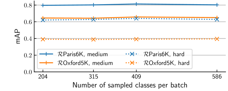
Figure 5: mAP for different batch sizes $B$. Best results are obtained with large batch sizes.

Figure 6: Assuming that it could be beneficial for the model to see images from different classes at each iteration, we construct each batch by sampling images from a limited random set of classes. This has little to no effect on the final performance.

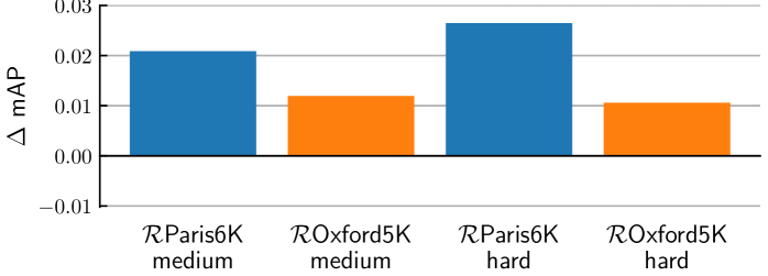
Figure 7: Balancing AP weights when computing the AP loss, such that all classes are weighted equally within a batch, brings a performance improvement of 1 to 3%.

Table 1: Ceteris paribus analysis on the loss.

	Medium			Hard			Number of Backwards	Number of Forwards	Number of Updates	Number of hyper-param.‡	Extra lines of code	Training time
Method	$\mathcal{R}$Oxf	$\mathcal{R}$Par		$\mathcal{R}$Oxf	$\mathcal{R}$Par
GeM (AP) [ours]	67.4	80.4		42.8	61.0		819K	1638K	200	2	15	1 day
GeM (TL-64) [ours]	64.9	78.4		41.7	58.7		1572K	2213K	8192	6	175 (HNM)	3 days
GeM (TL-512) [ours]	65.8	77.6		41.3	57.1		2359K	3319K	1536	6	175 (HNM)	3 days
GeM (TL-1024) [ours]	65.5	78.6		41.1	59.1		3146K	4426K	1024	6	175 (HNM)	3 days
R-MAC (TL)† [17]	60.9	78.9		32.4	59.4		1536K	3185K	8000	6	100+ (HNM)	4 days
GeM (CL)† [46]	64.7	77.2		38.5	56.3		1260K	3240K	36000	7	46 (HNM)	2.5 days

• ^†For the sake of completeness, we include metrics from [17] and [46] in the last two rows of the table even though they are not exactly comparable due the usage of different training sets or whitening and pooling mechanisms. ^‡See supplementary material for a listing of those parameters.

Score quantization.

Our $\text{mAP}_{\text{Q}}$ loss depends on the number of quantization bins $M$ in Eq. (7). We plot the performance achieved for different values of $M$ in Fig. 6. In agreement to previous findings [24, 58], this parameter has little impact on the performance. We use $M=20$ quantization bins in all other experiments.

Descriptor whitening.

As it is common practice [28, 44], we whiten our descriptors before evaluation. First, we learn a PCA from descriptors extracted from the Landmarks dataset. Then, we use it to normalize the descriptors for each benchmark dataset. As in [28], we use a square-rooted PCA. We use whitening in all subsequent experiments.

4.3 Ceteris paribus analysis

In this section, we study in more details the benefits of using the proposed listwise loss with respect to a state-of-the-art loss. For this purpose, we replace in our approach the proposed $\text{mAP}_{\text{Q}}$ loss by the triplet loss (TL) accompanied by hard negative mining (HNM) as described in [17] (i.e. using batches of 64 triplets). We then re-train the model, keeping the pipeline identical and separately re-tuning all hyper-parameters, such as the learning rate and the weight decay. Performance after convergence is presented in the first two lines of Table 1. Our implementation of the triplet loss, denoted as “GeM (TL-64)”, is on par or better than [17], which is likely due to switching from R-MAC to GeM pooling [46]. More importantly, we observe a significant improvement when using the proposed $\text{mAP}_{\text{Q}}$ loss (up to 3% mAP) even though no hard-negative mining scheme is employed. We stress that training with the triplet loss using larger batches (i.e. seeing more triplets before updating the model), denoted as GeM (TL-512) and GeM (TL-1024), does not lead to increased performance as shown in Table 1. Note that TL-1024 corresponds to seeing $1024\times 3=3072$ images per model update, which roughly corresponds to a batch size $B=4096$ with our $m\text{AP}_{\text{Q}}$ loss. This shows that the good performance of the $\text{mAP}_{\text{Q}}$ loss is not solely due to using larger training batches.

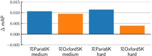
Figure 8: Improvement in mAP from mean $\text{mAP}_{\text{T}}$ loss to mean $\text{mAP}_{\text{Q}}$ loss. Our AP formulation results in a small but constant improvement with respect to the tie-aware AP formulation from [23].

We also indicate in Table 1 the training effort for each method (number of backward and forward passes, number of updates, total training time) as well as the number of hyper-parameters and extra lines of code they require with respect to a base implementation (see supplementary material for more details). As it can be observed, our approach leads to considerably fewer weight updates than when using a local loss. It also leads to a significant reduction in forward and backward passes. This supports our claim that considering all images at once with a listwise loss is much more effective. Overall, our model is trained 3 times faster than with a triplet loss.

The methods can also be compared regarding the amount of engineering involved. For instance, hard negative mining can easily require hundreds of additional lines, and comes with many extra hyper-parameters. In contrast, the PyTorch code for the proposed backprop is only 5 lines longer than a normal backprop, the AP loss itself can be implemented in 10 lines, and our approach requires only 2 hyper-parameters (the number of bins $M$ and batch size $B$), that have safe defaults and are not very sensitive to changes.

4.4 Comparison with the state of the art

Table 2: Performance evaluation (mean average precision) for $\mathcal{R}$Oxford and $\mathcal{R}$Paris.

	Medium					Hard
	$\mathcal{R}$Oxf	$\mathcal{R}$Oxf+1M	$\mathcal{R}$Par	$\mathcal{R}$Par+1M		$\mathcal{R}$Oxf	$\mathcal{R}$Oxf+1M	$\mathcal{R}$Par	$\mathcal{R}$Par+1M
Local descriptors
HesAff-rSIFT-ASMK∗ + SP [44]	60.6	46.8	61.4	42.3		36.7	26.9	35.0	16.8
DELF-ASMK∗ + SP [41]	67.8	53.8	76.9	57.3		43.1	31.2	55.4	26.4
Global representations
MAC (O) [56]	41.7	24.2	66.2	40.8		18.0	5.7	44.1	18.2
SPoC (O) [3]	39.8	21.5	69.2	41.6		12.4	2.8	44.7	15.3
CroW (O) [30]	42.4	21.2	70.4	42.7		13.3	3.3	47.2	16.3
R-MAC (O) [56]	49.8	29.2	74.0	49.3		18.5	4.5	52.1	21.3
R-MAC (TL) [17]	60.9	39.3	78.9	54.8		32.4	12.5	59.4	28.0
GeM (O) [46]	45.0	25.6	70.7	46.2		17.7	4.7	48.7	20.3
GeM (CL) [46]	64.7	45.2	77.2	52.3		38.5	19.9	56.3	24.7
GeM (AP) [ours]	67.5	47.5	80.1	52.5		42.8	23.2	60.5	25.1
Query expansion
R-MAC (TL) + $\alpha$QE [17]	64.8	45.7	82.7	61.0		36.8	19.5	65.7	35.0
GeM (CL) + $\alpha$QE [46]	67.2	49.0	80.7	58.0		40.8	24.2	61.8	31.0
GeM (AP) + $\alpha$QE [ours]	71.4	53.1	84.0	60.3		45.9	26.2	67.3	32.3

• All global representations are learned from a ResNet-101 backbone, with varying pooling layers and fine-tuning losses. Abbreviations: (O) off-the-shelf features; (CL) fine-tuned with contrastive loss; (TL) fine-tuned with triplet loss; (AP) fine-tuned with mAP loss (ours); (SP) spatial verification with RANSAC; ($\alpha$QE) weighted query expansion [46].

We now compare the results obtained by our model with the state of the art. The top part of Table 2 summarizes the performance of the best-performing methods on the datasets listed in section 4.1 without query expansion. We use the notation of [44] as this helps us to clarify important aspects about each method. Namely, generalized-mean pooling [46] is denoted by GeM and the R-MAC pooling [56] is denoted by R-MAC. The type of loss function used to train the model is denoted by (CL) for the contrastive loss, (TL) for the triplet loss, (AP) for our $\text{mAP}_{\text{Q}}$ loss, and (O) if no loss is used (i.e. off-the-shelf features).

Overall, our model outperforms the state of the art by 1% to 5% on most of the datasets and protocols. For instance, our model is more than 4 points ahead of the best reported results [46] on the hard protocol of $\mathcal{R}$Oxford and $\mathcal{R}$Paris. This is remarkable since our model uses a single scale at test time (i.e. the original test images), whereas other methods boost their performance by pooling image descriptors computed at several scales. In addition, our network does not undergo any special pre-training step (we initialize our networks with ImageNet-trained weights), again unlike most competitors from the state of the art. Empirically we observe that the $\text{mAP}_{\text{Q}}$ loss renders such pre-training stages obsolete. Finally, the training time is also considerably reduced: training our model from scratch takes a few hours on a single P40 GPU. Our models will be made publicly available to download upon acceptance.

We also report results with query expansion (QE) at the bottom of Table 2, as is common practice in the literature [2, 17, 44, 46]. We use the $\alpha$-weighted versions [46] with $\alpha=2$ and $k=10$ nearest neighbors. Our model with QE outperforms other methods also using QE in 6 protocols out of 8. We note that our results are on par with those of the method proposed by Noh et al.  [41], which is based on local descriptors. Even though our method relies on global descriptors, hence lacking any geometric verification, it still outperforms it on the $\mathcal{R}$Oxford and $\mathcal{R}$Paris datasets without added distractors.

5 Conclusion

In this paper, we proposed the application of a listwise ranking loss to the task of image retrieval. We do so by directly optimizing a differentiable relaxation of the mAP, that we call $\text{mAP}_{\text{Q}}$. In contrast to the standard loss functions used for this task, $\text{mAP}_{\text{Q}}$ does not require expensive mining of image samples or careful pre-training. Moreover, we train our models efficiently using a multistaged optimization scheme that allows us to learn models on high-resolution images with arbitrary batch sizes, and achieve state-of-the-art results in multiple benchmarks. We believe our findings can guide the development of better models for image retrieval by showing the benefits of optimizing for the target metric. Our work also encourages the exploration of image retrieval beyond the instance level, by leveraging a metric that can learn from a ranked list of arbitrary size at the same time, instead of relying on local rankings.

References

- [1] R. Arandjelović, P. Gronat, A. Torii, T. Pajdla, and J. Sivic. NetVLAD: CNN architecture for weakly supervised place recognition. CoRR, abs/1511.07247, 2015.
- [2] R. Arandjelovic and A. Zisserman. Three things everyone should know to improve object retrieval. In CVPR, 2012.
- [3] A. Babenko and V. Lempitsky. Aggregating local deep features for image retrieval. In ICCV, 2015.
- [4] A. Babenko, A. Slesarev, A. Chigorin, and V. Lempitsky. Neural codes for image retrieval. In ECCV, 2014.
- [5] A. Behl, P. Mohapatra, C. V. Jawahar, and M. P. Kumar. Optimizing average precision using weakly supervised data. IEEE TPAMI, 2015.
- [6] C. Burges, T. Shaked, E. Renshaw, A. Lazier, M. Deeds, N. Hamilton, and G. Hullender. Learning to rank using gradient descent. In ICML, 2005.
- [7] F. Cakir, K. He, S. A. Bargal, and S. Sclaroff. MIHash: Online hashing with mutual information. In ICCV, 2017.
- [8] Z. Cao, T. Qin, T.-Y. Liu, M.-F. Tsai, and H. Li. Learning to rank: from pairwise approach to listwise approach. In ICML, 2007.
- [9] H. Chen, Y. Wang, Y. Shi, K. Yan, M. Geng, Y. Tian, and T. Xiang. Deep transfer learning for person re-identification. In International Conference on Multimedia Big Data, 2018.
- [10] W. Chen, X. Chen, J. Zhang, and K. Huang. Beyond triplet loss: a deep quadruplet network for person re-identification. In CVPR, 2017.
- [11] W. Chen, X. Chen, J. Zhang, and K. Huang. A multi-task deep network for person re-identification. In AAAI, 2017.
- [12] C. Corbiere, H. Ben-Younes, A. Ramé, and C. Ollion. Leveraging weakly annotated data for fashion image retrieval and label prediction. In ICCVW, 2017.
- [13] G. Csurka, C. Dance, L. Fan, J. Williamowski, and C. Bray. Visual categorization with bags of keypoints. In ECCVW, 2004.
- [14] F. Faghri, D. J. Fleet, J. R. Kiros, and S. Fidler. VSE++: Improving visual-semantic embeddings with hard negatives. In BMVC, 2018.
- [15] Y. Gong, S. Lazebnik, A. Gordo, and F. Perronnin. Iterative quantization: A procrustean approach to learning binary codes for large-scale image retrieval. IEEE TPAMI, 2013.
- [16] A. Gordo, J. Almazán, J. Revaud, and D. Larlus. Deep image retrieval: Learning global representations for image search. In ECCV, 2016.
- [17] A. Gordo, J. Almazán, J. Revaud, and D. Larlus. End-to-end learning of deep visual representations for image retrieval. IJCV, 2017.
- [18] A. Gordo, J. A. Rodriguez-Serrano, F. Perronnin, and E. Valveny. Leveraging category-level labels for instance-level image retrieval. In CVPR, 2012.
- [19] I. Guy, A. Nus, D. Pelleg, and I. Szpektor. Care to share?: Learning to rank personal photos for public sharing. In International Conference on Web Search and Data Mining, 2018.
- [20] B. Hardwood, V. Kumar B G, G. Carneiro, I. Reid, and T. Drummond. Smart mining for deep metric learning. In ICCV, 2017.
- [21] B. Harwood, G. Carneiro, I. Reid, and T. Drummond. Smart mining for deep metric learning. In ICCV, 2017.
- [22] T. Hazan, J. Keshet, and D. A. McAllester. Direct loss minimization for structured prediction. In NIPS, 2010.
- [23] K. He, F. Cakir, S. A. Bargal, and S. Sclaroff. Hashing as tie-aware learning to rank. In CVPR, 2018.
- [24] K. He, Y. Lu, and S. Sclaroff. Local descriptors optimized for average precision. In CVPR, 2018.
- [25] K. He, X. Zhang, S. Ren, and J. Sun. Deep residual learning for image recognition. In CVPR, 2016.
- [26] P. Henderson and V. Ferrari. End-to-end training of object class detectors for mean average precision. In ACCV, 2016.
- [27] A. Hermans, L. Beyer, and B. Leibe. In defense of the triplet loss for person re-identification. arXiv preprint, 2017.
- [28] H. Jégou and O. Chum. Negative evidences and co-occurences in image retrieval: The benefit of PCA and whitening. In ECCV. 2012.
- [29] H. Jégou and A. Zisserman. Triangulation embedding and democratic aggregation for image search. In CVPR, 2014.
- [30] Y. Kalantidis, C. Mellina, and S. Osindero. Cross-dimensional weighting for aggregated deep convolutional features. In ECCVW, 2016.
- [31] D. P. Kingma and J. Ba. Adam: A method for stochastic optimization. arXiv preprint, 2014.
- [32] K. Kishida. Property of average precision and its generalization: An examination of evaluation indicator for information retrieval experiments. NII Technical Reports, 2005.
- [33] T. Liu. Learning to Rank for Information Retrieval. Springer, 2011.
- [34] T.-Y. Liu et al. Learning to rank for information retrieval. Foundations and Trends in Information Retrieval, 2009.
- [35] Z. Liu, P. Luo, S. Qiu, X. Wang, and X. Tang. DeepFashion: Powering robust clothes recognition and retrieval with rich annotations. In CVPR, 2016.
- [36] D. G. Lowe. Distinctive image features from scale-invariant keypoints. IJCV, 2004.
- [37] R. Manmatha, C.-Y. Wu, A. J. Smola, and P. Krähenbühl. Sampling matters in deep embedding learning. In ICCV, 2017.
- [38] A. Mishchuk, D. Mishkin, F. Radenović, and J. Matas. Working hard to know your neighbor’s margins: Local descriptor learning loss. In NIPS, 2017.
- [39] P. Mohapatra, C. Jawahar, and M. P. Kumar. Efficient optimization for average precision SVM. In NIPS, 2014.
- [40] Y. Movshovitz-Attias, A. Toshev, T. K. Leung, S. Ioffe, and S. Singh. No fuss distance metric learning using proxies. In ICCV, 2017.
- [41] H. Noh, A. Araujo, J. Sim, T. Weyand, and B. Han. Large-scale image retrieval with attentive deep local features. In ICCV, 2017.
- [42] J. Philbin, O. Chum, M. Isard, J. Sivic, and A. Zisserman. Object retrieval with large vocabularies and fast spatial matching. In CVPR, 2007.
- [43] J. Philbin, O. Chum, M. Isard, J. Sivic, and A. Zisserman. Lost in quantization: Improving particular object retrieval in large scale image databases. In CVPR, 2008.
- [44] F. Radenović, A. Iscen, G. Tolias, Y. Avrithis, and O. Chum. Revisiting Oxford and Paris: Large-scale image retrieval benchmarking. In CVPR, 2018.
- [45] F. Radenović, G. Tolias, and O. Chum. CNN image retrieval learns from BoW: Unsupervised fine-tuning with hard examples. In ECCV, 2016.
- [46] F. Radenović, G. Tolias, and O. Chum. Fine-tuning CNN image retrieval with no human annotation. TPAMI, 2018.
- [47] A. S. Razavian, H. Azizpour, J. Sullivan, and S. Carlsson. CNN features off-the-shelf: An astounding baseline for recognition. In CVPRW, 2014.
- [48] O. Rippel, M. Paluri, P. Dollar, and L. Bourdev. Metric learning with adaptive density discrimination. In ICLR, 2016.
- [49] O. Russakovsky, J. Deng, H. Su, J. Krause, S. Satheesh, S. Ma, Z. Huang, A. Karpathy, A. Khosla, M. Bernstein, A. C. Berg, and L. Fei-Fei. ImageNet large scale visual recognition challenge. IJCV, 2015.
- [50] F. Schroff, D. Kalenichenko, and J. Philbin. FaceNet: A unified embedding for face recognition and clustering. In CVPR, 2015.
- [51] H. Shi, Y. Yang, X. Zhu, S. Liao, Z. Lei, W. Zheng, and S. Z. Li. Embedding deep metric for person re-identification: A study against large variations. In ECCV, 2016.
- [52] K. Sohn. Improved deep metric learning with multi-class -pair loss objective. In NIPS, 2016.
- [53] H. O. Song, Y. Xiang, S. Jegelka, and S. Savarese. Deep metric learning via lifted structured feature embedding. In CVPR, 2016.
- [54] Y. Song, A. Schwing, Richard, and R. Urtasun. Training deep neural networks via direct loss minimization. In ICML, 2016.
- [55] E. Spyromitros-Xioufis, S. Papadopoulos, I. Y. Kompatsiaris, G. Tsoumakas, and I. Vlahavas. A comprehensive study over VLAD and product quantization in large-scale image retrieval. IEEE Transactions on Multimedia, 2014.
- [56] G. Tolias, R. Sicre, and H. Jégou. Particular object retrieval with integral max-pooling of CNN activations. In ICLR, 2016.
- [57] A. Trotman. Learning to rank. Information Retrieval, 2005.
- [58] E. Ustinova and V. Lempitsky. Learning deep embeddings with histogram loss. In NIPS. 2016.
- [59] C. Wang, X. Lan, and X. Zhang. How to train triplet networks with 100k identities? In ICCVW, 2017.
- [60] W. Wang, Y. Xu, J. Shen, and S.-C. Zhu. Attentive fashion grammar network for fashion landmark detection and clothing category classification. In CVPR, 2018.
- [61] Y. Yue, T. Finley, F. Radlinski, and T. Joachims. A support vector method for optimizing average precision. In SIGIR, 2007.