11email: {ripanaquec,rvelezmorol,rurbinag}@unp.edu.pe
Bspline solids manipulation with Mathematica
Abstract
Bspline solids are used for solid objects modeling in . Mathematica incorporates a several commands to manipulate symbolic and graphically Bspline basis functions and to graphically manipulate Bsplines curves and surfaces; however, it does not incorporate any command to the graphical manipulation of Bspline solids. In this paper, we describe a new Mathematica program to compute and plotting the Bspline solids. The output obtained is consistent with Mathematica’s notation. The performance of the commands are discussed by using some illustrative examples.
Keywords:
Make mesh, Make polyhedrons, Solids, BSpline solids.1 Introduction
Currently, Bspline solids are extensively used for solid objects modeling in [3, 5, 6, 7]. The most popular and widely used symbolic computation program, Mathematica [8], incorporates a several commands to manipulate symbolic and graphically Bspline basis functions and to graphically manipulate Bspline curves and surfaces [1, 2]; however, it does not incorporate any command to the graphical manipulation of Bspline solids.
In this paper, we describe a new Mathematica command: BSplineSolid (which defines a graphics object), to plotting the Bspline solids. Both commands are coded based on the code that displays R. Maeder [4] and commands that incorporates Mathematica [1], for that reason its options supported come to be the same as those commands in which them are based. The commands have been implemented in Mathematica v.11.0 although later releases are also supported. The output obtained is consistent with Mathematica’s notation.
The structure of this paper is as follows: Section 2 provides some mathematical background on Bspline basis, Bspline curves, Bspline surfaces and Bspline solids. Then, Section 3 describes the main standard Mathematica tools for Bsplines manipulation. Finally, Section 4 introduces the new Mathematica commands for manipulating them. The performance of the commands are discussed by using some illustrative examples.
2 Mathematical Preliminaries
An order Bspline is formed by joining several pieces of polynomials of degree with at most continuity at the breakpoints. A set of nondescending breaking points defines a knot vector
which determines the parametrization of the basis functions.
Given a knot vector , the associated Bspline basis functions, , are defined as:
for , and
for and .
The Bspline curve is defined by a set of control points , and a knot vector associated with the parameter . The corresponding Bspline curve is given by
A NURBS curve can be represented as
where is a weighting factor. If all , the Bspline curve is recovered.
The Bspline surface is a tensor product surface defined by a topologically rectangular set of control points , , and two knot vectors and associated with each parameter . The corresponding Bspline surface is given by
A NURBS surface can be represented as
where is a weighting factor. If all , the Bspline surface is recovered.
The Bspline solid is a tensor product solid defined by a topologically paralelepepidal set of control points , , , and three knot vectors , and associated with each parameter . The corresponding Bspline solid is given by
A NURBS solid can be represented as
where is a weighting factor. If all , the Bspline solid is recovered.
3 Standard Mathematica tools for Bspline manipulation
The command
BSplineBasis[]
gives the non-uniform B-spline basis function of degree with knots at positions .
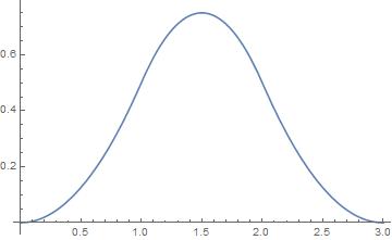
Below are two examples of base functions, in and , generated with the BsplineBasis command.
In[1]:=U={0,0,0,1,2,3,3,3};
       Plot[BSplineBasis[{2,U},2,u],{u,0,3}]
See Figure 1.
In[3]:=U=V={0,0,0,1,2,3,3,3};
       Plot3D[BSplineBasis[{2,U},2,u] BSplineBasis[{2,V},2,v],
        {u,0,3},{v,0,3},PlotRange->All]
See Figure 1.
The command
BSplineCurve[]
is a graphics primitive that represents a nonuniform rational B-spline curve with control points . This command incorporates the options
SplineKnots, SplineWeights, SplineDegree and SplineClosed
The first three options allow to control the knot vector, the weights and the degree (respectively) that define the Bspline curve. The last option allows defining a closed Bspline curve.
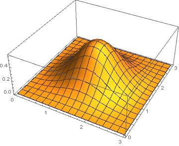
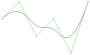
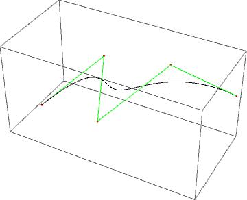
The two examples shown below correspond to a Bspline curve in and another Bspline curve in .
In[5]:=pts={{0,0},{1,1},{2,-1},{3,0},{4,-2},{5,1}};
       Graphics[{BSplineCurve[pts],Green,Line[pts],Red,Point[pts]}]
See Figure 2.
In[7]:=pts={{0,0,0},{1,1,1},{2,-1,1},{3,0,2},{4,1,1}};
       Graphics3D[{BSplineCurve[pts],Green,Line[pts],Red,Point[pts]}]
See Figure 2.
The command
BSplineSurface[]
is a graphics primitive that represents a nonuniform rational B-spline surface defined by an array of control points. This command incorporates the same options as the BsplineCurve command.
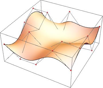
The following example shows a Bspline surface for an random array of control points.
In[9]:=cpts=Table[{i,j,RandomReal[{-1,1}]},{i,5},{j,5}];
       Graphics3D[{BSplineSurface[cpts],
        PointSize[Medium], Red, Map[Point, cpts], Gray, Line[cpts],
        Line[Transpose[cpts]]}]
See Figure 3.
4 Bspline solids manipulation
We will start this section by defining the MakeMesh [4] and MakePolyhedrons (new) commands to build a flat Bspline surface (entirely contained in a 2D space) and a spatial Bspline solid (entirely contained in a 3D space), respectively.
In[10]:=MakeMesh[vl_List]:=
         Block[{l=vl,l1=Map[RotateLeft,vl],mesh},
           mesh={l,l1,RotateLeft[l1],RotateLeft[l]};
           mesh=Map[Drop[#,-1]&,mesh,{1}];
           mesh=Map[Drop[#,-1]&,mesh,{2}];
           Transpose[Map[Flatten[#,1]&,mesh]]
           ]
In[12]:=MakePolyhedrons[vl_List]:=
         Block[{ mesh3d,newfaces,
             faces = {{1,2,3,4},{5,6,7,8},{1,2,6,5},
             {8,7,3,4},{2,3,7,6},{1,5,8,4}} },
           mesh3d=Map[MakeMesh,vl];
           mesh3d=
            Map[Flatten[#,1]&,Map[Thread,Partition[mesh3d,2,1]],{2}];
           mesh3d=Flatten[mesh3d,2];
           newfaces=Table[faces+8(i-1),{i,Length[mesh3d]/8}];
           GraphicsComplex[mesh3d,GraphicsGroup[Polygon/@newfaces]]
           ]
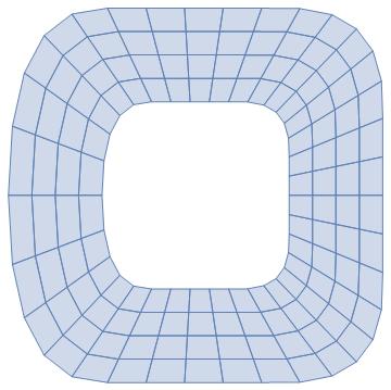
Next, the control points, the node vectors and the weights defining a flat Bspline surface are provided. Additionally, such a surface is plotted (Fig. 4). All this is done using the built-in Mathematica commands and the MakeMesh command.
In[13]:=points=
         {{{-2,0},{-3/2,0},{-1,0}},{{-2,-2},{-3/2,-3/2},{-1,-1}},
         {{0,-2},{0,-3/2},{0,-1}},{{2,-2},{3/2,-3/2},{1,-1}},
         {{2,0},{3/2,0},{1,0}},{{2,2},{3/2,3/2},{1,1}},
         {{0,2},{0,3/2},{0,1}},{{-2,2},{-3/2,3/2},{-1,1}},
         {{-2,0},{-3/2,0},{-1,0}}};
In[14]:={pp1,pp2}={35,5};
        {d1,d2}={2,2};
        {knots1,knots2}={{0,0,0,1,2,3,4,5,6,7,7,7},{0,0,0,1,1,1}};
        sw=Table[1,{i,n1},{j,n2}];
In[18]:=bssurf=Sum[sw[[i+1,j+1]]points[[i+1,j+1]]
         BSplineBasis[{d1,knots1},i,u]BSplineBasis[{d2,knots2},j,v],
         {i,0,n1-1},{j,0,n2-1}]/
         Sum[sw[[i+1,j+1]]
         BSplineBasis[{d1,knots1},i,u]BSplineBasis[{d2, knots2},j,v],
         {i,0,n1-1},{j,0,n2-1}];
In[19]:={u0,u1,v0,v1}={knots1[[d1+1]],knots1[[n1+d1 -1]],
          knots2[[d2+1]],knots2[[n2+d2-1]]};
        {du,dv}={(u1-u0)/(pp1-1.),(v1-v0)/(pp2-1.)};
        aux=Table[N[bssurf],{u,u0,u1,du},{v,v0,v1,dv}];
In[22]:=Graphics[{EdgeForm[RGBColor[0.36841,0.50677,0.70979]],
         Directive[RGBColor[0.36841,0.50677,0.70979],Opacity[0.3]],
         Polygon/@MakeMesh[aux]}]
See Figure 4 (left).
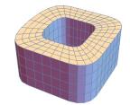
Then, control points, node vectors and weights that define a spatial Bspline solid are provided. In addition, such a solid is plotted (Fig. 4). All this is done using the built-in Mathematica commands and the MakePolyhedrons command.
In[23]:=points={{{{-2,0,0},{-3/2,0,0},{-1,0,0}},{{-2,-2,0},
            {-3/2,-3/2,0},{-1,-1,0}},{{0,-2,0},{0,-3/2,0},
            {0,-1,0}},{{2,-2,0},{3/2,-3/2,0},{1,-1,0}},
           {{2,0,0},{3/2,0,0},{1,0,0}},{{2,2,0},{3/2,3/2,0},
            {1,1,0}},{{0,2,0},{0,3/2,0},{0,1,0}},{{-2,2,0},
            {-3/2,3/2,0},{-1,1,0}},{{-2,0,0},{-3/2,0,0},{-1,0,0}}},
         {{{-2,0,1},{-3/2,0,1},{-1,0,1}},{{-2,-2,1},{-3/2,-3/2,1},
            {-1,-1,1}},{{0,-2,1},{0,-3/2,1},{0,-1,1}},{{2,-2,1},
            {3/2,-3/2,1},{1,-1,1}},{{2,0,1},{3/2,0,1},{1,0,1}},
           {{2,2,1},{3/2,3/2,1},{1,1,1}},{{0,2,1},{0,3/2,1},
            {0,1,1}},{{-2,2,1},{-3/2,3/2,1},{-1,1,1}},{{-2,0,1},
            {-3/2,0,1},{-1,0,1}}},{{{-2,0,2},{-3/2,0,2},{-1,0,2}},
           {{-2,-2,2},{-3/2,-3/2,2},{-1,-1,2}},{{0,-2,2},{0,-3/2,2},
            {0,-1,2}},{{2,-2,2},{3/2,-3/2,2},{1,-1,2}},{{2,0,2},
            {3/2,0,2},{1,0,2}},{{2,2,2},{3/2,3/2,2},{1,1,2}},
           {{0,2,2},{0,3/2,2},{0,1,2}},{{-2,2,2},{-3/2,3/2,2},
            {-1,1,2}},{{-2,0,2},{-3/2,0,2},{-1,0,2}}}};
In[24]:={n1,n2,n3,d}=Dimensions[points];
        {pp1,pp2,pp3}={5,35,5};
        {d1,d2,d3}={2,2,2};
        {knots1,knots2,knots3}={{0,0,0,1,1,1},
          {0,0,0,1,2,3,4,5,6,7,7,7},{0,0,0,1,1,1}};
        sw = Table[1,{i,n1},{j,n2},{k,n3}];
In[29]:=bssol=Sum[sw[[i+1,j+1,k+1]]points[[i+1,j+1,k+1]]
          BSplineBasis[{d1,knots1},i,u]BSplineBasis[{d2,knots2},j,v]
          BSplineBasis[{d3,knots3},k,w],
           {i,0,n1-1},{j,0,n2-1},{k,0,n3-1}]/
         Sum[sw[[i+1,j+1,k+1]]BSplineBasis[{d1,knots1},i,u]
          BSplineBasis[{d2,knots2},j,v]BSplineBasis[{d3,knots3},k, w],
          {i,0,n1-1},{j,0,n2-1},{k,0,n3-1}];
In[30]:={u0,u1,v0,v1,w0,w1}={knots1[[d1+1]],knots1[[n1+d1-1]],
         knots2[[d2+1]],knots2[[n2+d2-1]],knots3[[d3+1]],
         knots3[[n3+d3-1]]};
        {du,dv,dw}={(u1-u0)/(pp1-1.),(v1-v0)/(pp2-1.),
         (w1-w0)/(pp3-1.)};
        aux=Table[N[bssol],{u,u0,u1,du},{v,v0,v1,dv},{w,w0,w1,dw}];
In[33]:=Graphics3D[{EdgeForm[RGBColor[0.36841,0.50677,0.70979]],
         MakePolyhedrons[aux]},Boxed->False]
See Figure 4 (right).
By comparing the two previous processes it is possible to form an idea of the algorithm used to implement the main command, BSplineSolid.
Finally, we describe the Mathematica program we developed to compute the Bspline solids. For the sake of clarity, the program will be explained through some illustrative examples.
The BSplineSolid command is a graphics primitive that represents a nonuniform rational Bspline solid defined by an array of control points. The syntax of this command is:
The options supported by this command are: PlotPoints, SplineDegree, SplineKnots and SplineWeights.
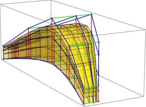
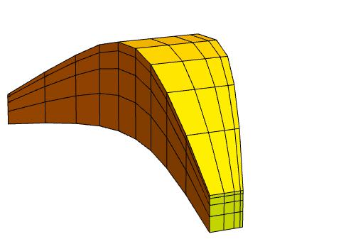
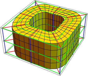
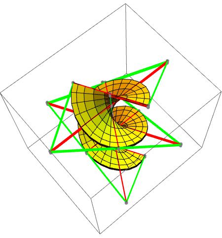
As a first example we compute the Bspline solid of order 2 for a set of points as follows:
In[34]:=pts=Table[{u,1/(1+u^2+v^2),1/(1+u^2+w^2)},
         {u,-1,1,1/2},{v,-1,1,1/2},{w,-1,1,1/2}];
In[35]:=Graphics3D[{Meshing[pts],Yellow,Opacity[0.2],BSplineSolid[pts]},
         ViewPoint->{3.,-1.6,0.8}]
See Figure 5 (left).
The Meshing command is defined as follows:
In[36]:=Meshing[pts_?ArrayQ]:={AbsolutePointSize[7],Gray,
         Map[Point,pts,{2}],Thick,Red,Map[Line[#] &,pts,{2}],
         Green,Map[Line[#]&,Transpose/@pts,{2}],
         Blue,Map[Line[#]&,Transpose/@Transpose[Transpose/@pts],{2}]}
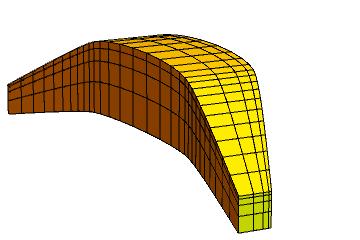
In[37]:=Graphics3D[{Yellow,BSplineSolid[pts]},
         ViewPoint->{3.,-1.6,0.8},Boxed->False]
See Figure 5 (right).
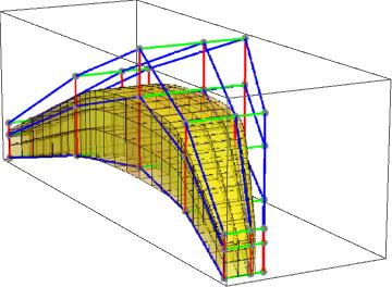
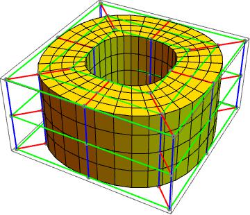
As a second example we compute the NURBS solid of order 2 for a set of points as follows:
In[38]:=w1={1,1,0.25,1,1};
        w3=w2=w1;
        w = Table[w1[[i]]w2[[j]]w3[[k]],{i,1,5},{j,1,5},{k,1,5}];
In[41]:=Graphics3D[{Meshing[pts],Yellow,Opacity[0.2],
         BSplineSolid[pts,SplineWeights->w,PlotPoints->{30,10,10}]},
         ViewPoint->{3.,-1.6,0.8}]
See Figure 6 (left).
In[42]:=Graphics3D[{Yellow,BSplineSolid[pts,SplineWeights->w,
          PlotPoints->{30,10,10}]},ViewPoint->{3.,-1.6,0.8},
         Boxed->False]
See Figure 6 (right).
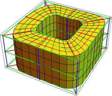
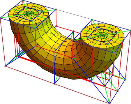
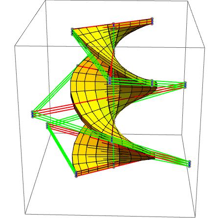
Moreover, figure 7 shows the adjustment process, by varying the node vectors and weights, modeling a solid hollow cylinder with NURBS solid. In practice this is achieved by changing the default values of options SplineWeights and SplineKnots. Similarly, seen in figure 8 the modeling a solid torus and in figure 9 the modeling a solid helix.


5 Conclusions
In this paper, we describe a new Mathematica program to compute and plotting the Bspline solids. The output obtained is consistent with Mathematica’s notation. The performance of the commands are discussed by using some illustrative examples.
6 Acknowledgements
The authors would like to thank to the authorities of the Universidad Nacional de Piura for the acquisition of the Mathematica 11.0 license and the reviewers for their valuable comments and suggestions.
References
- [1] Graphics Objects, https://reference.wolfram.com/language/howto/WorkWithSplineFunctions.html. Last accessed 17 Jan 2016
- [2] How to Work with Spline Functions, https://reference.wolfram.com/language/howto/WorkWithSplineFunctions.html. Last accessed 17 Jan 2016
- [3] Kim, J. H. and Lee, Y. J.: Trivariate B-spline approximation of spherical solid objects. Journal of information processing systems. 10(1), 23–35 (2014)
- [4] Maeder, R.: Programming in Mathematica (Second Edition). Addison-Wesley Longman Publishing Co., Inc., Boston, MA, USA (1991)
- [5] Ng-Thow-Hing, V. et al: Shape reconstruction and subsequent deformation of soleus muscle models using B-spline solid primitives. BiOS’98 International Biomedical Optics Symposium, Laval, France, 423–434 (1998)
- [6] Martin, T. et al: Volumetric parameterization and trivariate B-spline fitting using harmonic functions. Computer Aided Geometric Design. 26(6), 648–664 (2009)
- [7] Schmitt, B. et al: Constructive sculpting of heterogeneous volumetric objects using trivariate b-splines. The Visual Computer. 20(2-3), 130–148 (2016)
- [8] Wolfram, S.: The Mathematica Book (Fifth Edition). Wolfram Media (2003)