A Communication-less Protection Strategy to Ensure Protection Coordination of Distribution Networks with Embedded DG

Abstract

Distributed Generation (DG) has emerged as best alternative to conventional energy sources in recent times. Decentralization of power generation, improvement in voltage profile and reduction of system losses are some of key benefits of DG integration into the grid. However, introduction of DG changes the radial nature of a distribution network (DN) and may affect both magnitude and direction of fault currents. This phenomenon may have severe repercussions for the reliability and safety of a DN including protection coordination failure. This paper investigates the impact of DG on protection coordination of a typical DN and proposes a scheme to restore the protection coordination in presence of DG. Moreover, impact of different DG sizes and locations on DN’s voltage profile and losses has also been analyzed. The sample DN with embedded DG is modelled in ETAP environment and the simulation results presented show the effectiveness of the proposed protection strategy in restoring relay coordination of the network in both isolated and DG connected modes of operation.

I Introduction

The rapid increase in electrical energy demand combined with scarcity of fossil fuels and their high prices has made Distributed Generation (DG) based on renewable energy resources (RER) installed near to load centers as an attractive alternative. Recent advancement in renewable energy technologies is also one of the reasons for wide spread use of DG for electricity replacing generation from large centralized plants. Many studies focus on the selection of proper size and location of DG units as it may affect the voltage profile, total power loss and protective relay coordination, etc., of a distribution network (DN) [1, 2].

The objective of power system protection is to isolate the faulty part of the network from healthy part in case of fault. A good protection scheme should selective, fast, reliable, and sensitive [3]. Directional overcurrent relays (DOCRs) are widely described in literature for protection of distribution networks (DNs) with integrated DG due to their effectiveness and low price. There is an extensive literature that describes impact of DG on protection coordination of a DN and suggests various solutions based on both conventional as well as optimal techniques [4, 5, 6]. A protection coordination scheme is proposed in this paper that utilizes different time current characteristics (TCC) of microprocessor based relays to ensure protection coordination of a DN with embedded DG. TCCs that are selected for different relays hold good no matter whether DN is working with or without DG connection.

The remaining paper is arranged as under. Section II describes system modelling whereas section III contains protection design scheme for the original system without DG. The criteria for selection of size and location of DG is presented in Section IV. Section V contains impact of DG on protection coordination of the test system whereas section VI describes the proposed protection scheme for restoration of protection coordination in presence of DG. Section VII concludes the paper.

II System Modelling

Fig. 1 represents the Single Line Diagram(SLD) of Distribution Network modelled in ETAP which is modified version of Eastern Libyan Distribution Network [7]. The network comprises of three transformers and eleven buses. The grid is shown as an equivalent source with a short circuit capacity of 200 MVA connected at Bus 1. Table I enlists all system components along with their specifications. All the relays are directional except those connected with the grid and loads. The grid parameters are as shown in Fig 2.

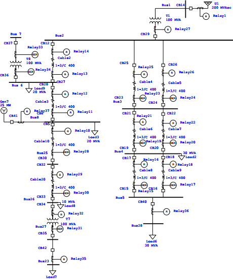
Figure 1: Single Line Diagram of Distribution Network

TABLE I: System Parameters

System Parameter	Specification
Transformer T1	100MVA, 220KV-30KV, Typical Z & X/R
Transformer T7	100MVA, 30KV-11KV Typical Z & X/R
Transformer T8	100MVA, 11.5KV-30KV, X/R=2.47 R/X=0.40, Z%=7, X%=6.48, R%=2.67,
Load 2	30MVA
Load 3	30MVA
Load 6	30MVA
Load 7	15MVA
Load 8	10MVA
Load 9	20MVA
Cable 2=8 KM, Cable 3=4KM, Cable 4=2.3KM= Cable 5, Cable 6=1.5KM= Cable7 Cable 8=3KM=Cable 9, Cable 10=5KM, Cable 20=8KM	Heesung XLPE 60 Hz, 30KV 400mm2, impedance calculated ohm/Km.
Relays (Overcurrent)	REF 542 plus
Breaker	High Voltage breaker

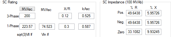
Figure 2: ETAP Parameter Settings for External Grid

Over-current protection scheme for the sample network is designed and tested in ETAP software with DG connected at bus 8. The DG size and location are selected on the basis of power loss reduction and improvement in voltage profile of the network. After DG integration, short circuit currents in the network increase and the existing protection scheme maloperates. To minimize the effect of DG on protection coordination, two potential solutions are investigated and simulated here. First solution is to redesign the protection scheme in the presence of DG by adaptively changing the relay settings [7, 8, 9]. In this case, relays will have two sets of settings; one setting for DG connected mode of operation and other for without DG connection. For implementation of this scheme, a communication link between DG and protective relays is necessary. Second solution is to change the characteristic curves of the relays that malfunction due to DG presence to ensure proper coordination between primary and back-up relays in both DG and without DG connection scenarios. Flowchart of methodology used is shown in Fig 3.

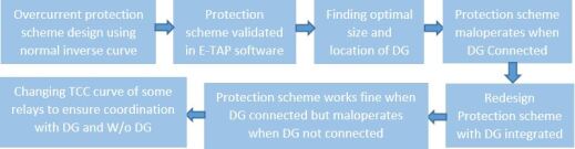
Figure 3: Methodology Flowchart

III Protection scheme design and coordination without DG in DN

A three phase bolted fault is simulated at different buses to determine the maximum fault currents for setting of DOCRs. Pick-up settings of the relays are calculated by allowing 25% overloading. The settings of DOCRs are based on standard inverse time characteristics [10].

$$Pickup=NormalLoadCurrent\times 1.25$$ (1)

$$PS=\frac{Pickup}{CTR}$$ (2)

Characteristic Equation For Standard Inverse Relay is;

$$T_{0}=\frac{0.14\times TMS}{(\frac{I_{f}}{CTR\times PS})^{0.02}-1}$$ (3)

where;
$T_{0}$ = Operating Time of Relay
CTR = Current Transformer Ratio
$I_{f}$ = Three Phase Fault Current through that Relay
PS = Plug Setting of Relay
TMS = Time Multiplier Setting
CTI = 200ms = Coordination Time Interval

III-A Calculation for Relay Setting At Bus 23

Upon careful observation of the simulated network, it can be noticed that for fault at Bus 23 $Relay_{35}$ is the primary relay and $Relay_{32}$ is its backup. TMS of $Relay_{35}$ is 0.05. From Equation 3 ;

$$T_{35}=\frac{0.14\times 0.05}{(\frac{6110}{1200\times 0.598})^{0.02}-1}=0.16sec$$ (4)

$$T_{35}=0.16sec$$

Also,

$$T_{32}=T_{35}+CTI=0.36sec$$

Time Multiplier Setting of $Relay_{32}$ is determined from Equation 3 as under;

$$TMS=\frac{T_{0}\times(\frac{I_{f}}{CTR\times PS})^{0.02}-1)}{0.14}$$ (5)

$$TMS_{32}=\frac{0.36\times(\frac{6110}{1200\times 0.275})^{0.02}-1)}{0.14}$$

$$TMS_{32}=0.15sec$$

III-B Protection Coordination Settings

The method described above has been used to determine the settings of DOCRs installed in the DN. Table II shows the setting of protection devices without DG. All the current transformers has a ratio of 1200:1.

TABLE II: Protection settings without DG

Bus	If (A)	Rp	Rb	Relay No	Type	PS	TMS
23	6110	35	32	35	Dir	0.598	0.05
27	2210	32	29	32	Dir	0.275	0.14
26	2330	29	10	29	Dir	0.848	0.126
25	2660	10	12	10	Dir	0.466	0.17
8	2910	12	14	12	Dir	0.831	0.18
6	3140	14	1	14	Dir	1.21	0.115
2	501	1	Nil	1	ND	0.324	0.19
28	3430	36	16,18	36	Dir	0.583	0.05
5	1720	16,18	21,22	16,18	Dir	0.291	0.135
4	1760	21,22	25,26	21,22	Dir	0.584	0.102
3	1790	25,26	1	25,26	Dir	0.585	0.128

III-C Relay Curves

Relay curves can be seen for faults at Bus 26 and Bus 27 in Fig. 4 and Fig. 5 respectively. For fault at Bus 26 $Relay_{29}$ is primary relay and $Relay_{10}$ is secondary relay. Similarly for Bus 27 $Relay_{32}$ is primary and $Relay_{29}$ is secondary relay. It can be seen that in both the cases, protection coordination is ensured as the value of CTI is close to required value of 200 ms as given in Equation 6 and Equation 7. Table III shows timing of various primary and backup relays of the network without DG connection. Abbreviations used in the Table are;

$$T_{relay10}-T_{relay29}=CTI=879ms-689ms=190ms$$

$$T_{relay29}-T_{relay32}=CTI=719ms-506ms=213ms$$

Figure 4: Relay TCC curves for fault at bus 26 without DG

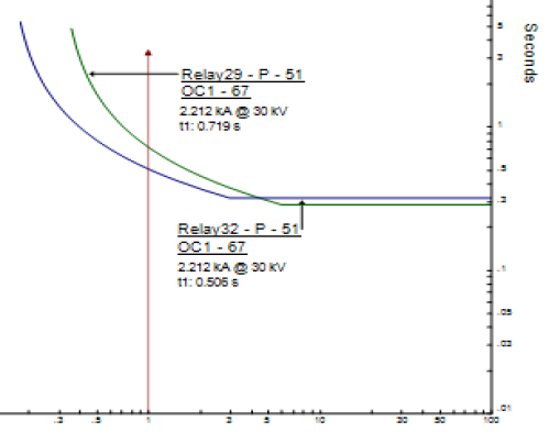
Figure 5: Relay TCC Curves for faut at bus 27 without DG

TABLE III: OPERATING TIMES WITHOUT DG CONNECTION

Fault at Bus	Rp	Rb	Tp	Tb	CTI(ms)	MC
23	35	32	161	506	345	Nil
27	32	29	506	719	213	Nil
26	29	10	689	889	200	Nil
25	10	12	751	951	200	Nil
8	12	14	889	1099	210	Nil
6	14	1	991	1500	509	Nil
2	1	36	1026	nil	Nil	Nil
28	36	16,18	218	585	367	Nil
5	16,18	21,22	583	934	351	Nil
4	21,22	25,26	904	1100	196	Nil
3	25,26	1	1165	1376	211	Nil

$R_{p}$=Primary Relay number $R_{b}$=Backup Relay number $T_{p}$=Primary Relay time $T_{b}$=Backup Relay time $CTI$=Coordination time interval $MC$=Miscoordination

IV Selection of DG Size and Location

From Table IV it can been seen that losses are reduced to 1109.7 KW from original 3849 KW after DG connection which shows an improvement of 68%. However, due to certain constraints, Bus 27 is not a feasible location for DG connection. So, Bus 8 which is next to Bus 27 in terms of loss reduction is selected for DG connection.

TABLE IV: Network Losses of the DN with DG at different locations

Bus No	DG Size	Losses (KW)	Bus No	DG Size	Losses (KW)
2	25	3560.1	5	25	3584.97
2	50	3560.1	5	50	3584.97
3	25	3477	25	25	1851.93
3	50	3477	25	50	1851.93
8	25	1683	26	25	1741.41
8	50	1683	26	50	1741
23	25	2037	27	25	1506
23	50	2037	27	50	1109.7
1	25	3849	28	25	2887
1	50	3849	28	50	2887
4	25	3366
4	50	3366

V Protection Coordination after Connection of DG

Major protection issues associated with integration of DG into a DN are change in direction and magnitude of fault current, blinding of protection and false tripping of relays etc. [11]. It can be seen in Fig. 6 and Fig. 7 that after DG integration, CTI is not ensured for faults at Bus 26 and Bus 27.

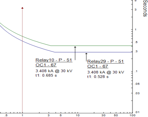
Figure 6: Relay TCC curves for fault at bus 26 with DG

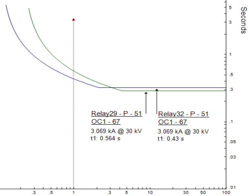
Figure 7: Relay TCC curves for fault at bus 27 with DG

For Bus 26:

$$T_{10}-T_{29}=CTI=685ms-528ms=157ms$$

As 157 ms is considerably smaller than 200 ms, so in this case CTI is not ensured.

Similarly, for Bus 27:

$$T_{29}-T_{32}=CTI=564ms-439ms=125ms$$

As 125 ms is considerably smaller than 200 ms, so CTI is not ensured in this case, too.

TABLE V: Primary and backup relay time with DG

Bus	If (A)	Rp	Rb	Tp	Tb	CTI(ms)	MC
23	8370	35	32	139	430	291	Nil
27	3070	32	29	430	560	130	Yes
26	3410	29	10	528	640	112	Yes
25	4300	10	12	572	1022	450	Nil
8	2910	12	14	889	1099	210	Nil
6	3140	14	1	991	1540	549	Nil
2	501	1	36	1350	Nil	Nil	Nil
28	4580	36	16,18	184	493	309	Nil
5	2290	16,18	21,22	493	704	211	Nil
4	2420	21,22	25,26	675	875	200	Nil
3	2470	25,26	1	863	1397	534	Nil
6	2750	11	37	1356	1601	245	Nil
2	2370	13	11	1490	1680	190	Nil
8	2970	37	Nil	2586	Nil	Nil	Nil
1	2110	27	13	214	1600	1386	Nil

From Table V, it can be seen that miscoordination of relays occur when fault is introduced at Bus 26 and Bus 27 which needs to be corrected.

VI Methods to solve Protection Coordination problems after DG integration

VI-A Protection Redesign in the Presence of DG

In order to regain protection coordination between primary and backup relays, we redesigned the protection settings in the presence of DG. DG integration in to system have increased the short circuit current levels that is the source of miscoordination between primary and backup relays. New TMS and PS of the relays are calculated in exactly the same manner as was used for the protection settings of DN without DG. Redesigned protection settings works fine in the presence of DG but at the time when DG is removed, some relays maloperate. So the coordination problem remains still unresolved. New protection settings are shown in Table VI

TABLE VI: Redesign protection settings of DN with DG of 25MW at Bus 8

Fault at Bus No	If (A)	PS	TMS
23	8370	0.599	0.05
27	3070	0.276	0.117
26	3410	0.549	0.129
26	4300	0.466	0.199
8	2910	0.831	0.159
23	3140	1.21	0.127
2	501	0.116	0.04
28	4580	0.588	0.05
5	2290	0.291	0.135
4	2420	0.584	0.121
3	2470	0.585	0.157
11	2750	0.744	0.089
13	2370	0.358	0.096
37	2970	1.63	0.042
27	2110	0.351	0.05

VI-B Changing Characteristic Curves of Relays

The second solution that is, changing characteristic curve of the relays that malfuntion, is adopted here to restore protection irrespective of DG connection status. Available Curves for relay REF542plus are

VI-B1 Normal Inverse

VI-B2 Extremely inverse

VI-B3 Very inverse

VI-B4 Long inverse

$$T_{0}=\frac{a\times TMS}{(\frac{I_{f}}{CTR\times PS})^{b}-1}$$ (6)

Table VII shows parameters ’a’ and ’b’ for different types of curves. There are also some special type of curves like RI type and RXIDG type which are used where high selectivity is required. Relays time are calculated using extremly inverse and very inverse in Table VIII and IX respectively.

TABLE VII: Relay Characteristic Curves formulas

Degree of inversity of the Relay	a	b
Normal Inverse	0.02	0.14
Very Inverse	1	13.5
Extremely inverse	2	80

TABLE VIII: Extremely Inverse Case

Fault at Bus No	Tp	Ts	CTI	MS
23	60	112	62	Yes
27	112	386	274	nil
26	310	443	133	Yes
25	300	1300	1000	nil
8	2126	1000	1126	nil
6	473	4000	3527	nil
2	6000			nil
28	97.2	405	307.2	nil
5	405	818	413	nil
4	743	1467	724	T13=313
3	1384	6400	5016	T13=296,T11=729

TABLE IX: Very Inverse Case

Fault at Bus No	Tp	Ts	CTI	MS
23	63.4	179	115.6	Yes
27	179	379	200	Nil
26	323	530	207	Nil
25	404	1874	1470	Nil
8	1406	1343	-63	Yes
6	1162	2700	1538	Nil
2	300	2700	2400	Nil
28	123	503	380	Nl
5	504	600	96	Yes
4	550	1102	552	T13=325
3	1072	2700	1628	T13=315,T11=437

It can be seen from Table VIII and IX that when the characteristic curves of all relays are changed from normal inverse to extremely and very inverse even then miscoordination occurs. Not a single characteristic curve could fix the mis-coordination problem. So, a strategy to change curves of only those relays that maloperate, from normal inverse to extreme and very inverse has been used to ensure coordination.

In table X and XI , it is shown that by changing the characteristic curve of some relays have solved the problem of mis-coordination between primary and backup relays for both cases, without and with DG connection, as CTI is now higher than 200ms. Table XI shows Characteristic curve of different relays, which ensures coordination with DG and without DG case.

TABLE X: Changing Characteristic curve in without dg case

Bus	Rp	Rb	Tp	Tb	CTI	MC
23	35	32	57.6	333	275.4	Nil
27	32	29	333	722	389	Nil
26	29	10	670	918	248	Nil
25	10	12	839	1057	218	Nil
8	12	14	988	1199	211	Nil
6	14	1	1061	1540	479	Nil
2	1	36	1350	Nil	Nil	Nil
28	36	16,18	218	585	367	Nil
5	16,18	21,22	585	934	349	Nil
4	21,22	25,26	904	1175	271	Nil
3	25,26	1	1156	1376	220	Nil

TABLE XI: Changing Characteristic curve in with dg case

Bus	Rp	Rb	Tp	Tb	CTI	MC
23	35	32	29.7	229	199.3	Nil
27	32	29	229	465	236	Nil
26	29	10	408	723	315	Nil
25	10	12	639	1100	461	Nil
8	12	14	988	1199	211	Nil
6	14	1	1081	1600	519	Nil
2	1	36	1350	Nil	Nil	Nil
28	36	16,18	184	493	309	Nil
5	16,18	21,22	493	704	211	Nil
4	21,22	25,26	675	876	201	Nil
3	25,26	1	858	1937	1079	Nil

TABLE XII: Characteristic Curves of Relays

Relay No	Characteristic Curve	Relay No	Characteristic Curve
35	Extremely Inverse	36	Normal inverse
32	Very Inverse	16,18	Normal inverse
29	Very Inverse	21,22	Normal inverse
10	Normal inverse	25,26	Normal inverse
12	Normal inverse	11	Normal inverse
14	Normal inverse	13	Normal inverse
1	Normal inverse	37,27	Normal inverse

Figure 8: Relay Curves without DG when fault at bus 27

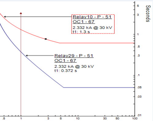
Figure 9: Relay Curves without DG when fault at bus 26

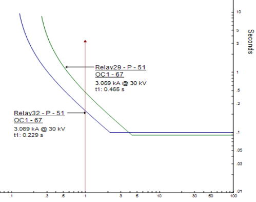
Figure 10: Relay Curves with DG when fault at bus 27

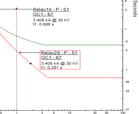
Figure 11: Relay Curves with DG when fault at bus 26

In Fig 8 and 9 relay TCC curves are shown in case of without DG for bus fault 27 and 26 respectively. Similarly Fig 10 and 11 shows TCC curves in with DG case. In both cases CTI is insured between primary and backup relays.

VII Conclusion

The study shows that in some circumstances, it may not be possible to keep and restore coordination of DOCRs in presence of DG. A solution is proposed based on selection of different time current characteristics curves for the DOCRs installed in the network. A sample network is modeled in ETAP environment and through simulation results it is shown that it is possible to retain the original protection coordination through intelligent selection of characteristics curves for the system relays.

References

[1]
A.K. Singh, S.K. Parida, ‘A review on distributed generation allocation and planning in deregulated electricity market’, Pages 1969-4344 (February 2018), Renewable and sustainable Energy Reviews.
[2]
P.S. Georgilakis, N.D. Hatziargyriou, ‘Optimal Distributed Generation Placement in Power Distribution Networks: Models, Methods, and Future Research’, IEEE Transactions on Power Systems, 28 (3) (2013), pp. 3420-3428.
[3]
P. M. Anderson, Power System Protection. New York: IEEE, 1998.
[4]
P. P. Barer, R. W. De Mello, ”Determining the impact of distributed generation on power system: par 1 - radial distribution systems”, IEEE Power Engineering Society vol. 3, pp. 1645-1656, (2000).
[5]
Martin Geidl, ”Protection of Power Systems withDistributed Generation: State of the Art”, Power Systems Laboratory, ETH Zurich, (2005).
[6]
Ehrenberger, J.; Švec, J., Anang Tjahjono , Dimas O. Anggriawan, et. al ‘Adaptive modified firefly algorithm for optimal coordination of overcurrent relays’, IET Gener. Transm. Distrib., 2017, Vol. 11 Iss. 10, pp. 2575-2585.
[7]
S. M. Saad, N. El Naily, A. Elhaffar, K. El-Arroudi, and F. A. Mohamed, “Applying adaptive protection scheme to mitigate the impact of distributed generator on existing distribution network,” IREC, 2017, pp. 1–6.
[8]
S. Acharya, S. K. Jha, R. Shrestha, A. Pokhrel, and B. Bohara, “An analysis of time current characteristics of adaptive inverse definite minimum time (IDMT) overcurrent relay for symmetrical and un-symmetrical faults,” ICSPACE, 2017, pp. 332–337.
[9]
S. C. Ilik and A. B. Arsoy, “Effects of Distributed Generation on
Overcurrent Relay Coordination and an Adaptive Protection Scheme,” IOP Conf. Series: Earth and Environ. Science, vol. 73, p. 012026, 2017.
[10]
IEEE, “IEEE Standard Inverse-Time Characteristic Equations for Overcurrent Relays,” IEEE Standard C37.112-1996, Jul. 1999.
[11]
M. H. J. Bollen, “Integration of distributed generation in the power system. Hoboken,” N.J: Wiley-IEEE Press, 2011.
[12]
Y. G. Paithankar and S. R. Bhide, “Fundamentals of power system protection,” New Delhi: Prentice-Hall of India, 2007.