Comparative terrestrial atmospheric circulation regimes in simplified global circulation models: I. from cyclostrophic super-rotation to geostrophic turbulence

Abstract

The regimes of possible global atmospheric circulation patterns in an Earth-like atmosphere are explored using a simplified GCM based on the University of Hamburg’s Portable University Model for the Atmosphere (PUMA) — with simplified (linear) boundary layer friction, a Newtonian cooling scheme and dry convective adjustment (designated here as PUMA-S). A series of controlled experiments are conducted by varying planetary rotation rate and imposed equator-to-pole temperature difference. These defining parameters are further combined with each other into dimensionless forms to establish a parameter space, in which the occurrences of different circulation regimes are mapped and classified. Clear, coherent trends are found when varying planetary rotation rate (thermal Rossby number) and frictional and thermal relaxation timescales. The sequence of circulation regimes as a function of parameters, such as the planetary rotation rate, strongly resembles that obtained in laboratory experiments on rotating, stratified flows, especially if a topographic $\beta$-effect is included in those experiments to emulate the planetary vorticity gradients in an atmosphere induced by the spherical curvature of the planet. A regular baroclinic wave regime is also obtained at intermediate values of thermal Rossby number and its characteristics and dominant zonal wavenumber depend strongly on the strength of radiative and frictional damping. These regular waves exhibit some strong similarities to baroclinic storms observed on Mars under some conditions. Multiple jets are found at the highest rotation rates, when the Rossby deformation radius and other eddy-related length scales are much smaller than the radius of the planet. These exhibit some similarity to the multiple zonal jets observed on gas giant planets. Jets form on a scale comparable to the most energetic eddies and the Rhines scale poleward of the supercritical latitude. The balance of heat transport varies strongly with $\Omega^{\ast}$ between eddies and zonally symmetric flows, becoming weak with fast rotation.

1 Introduction

An understanding of the dominant factors and mechanisms controlling the general circulation of a planetary atmosphere is a prerequisite to our understanding of the climate variability of the Earth, both in the past and in the future. This goal has stimulated an immense body of research during the past century, focussing particularly on the details of the Earth’s atmosphere, surface and planetary environment and the parameters which define them. From one viewpoint this is entirely understandable, since many aspects of the changing climate of the present day are manifested in relatively subtle ways through small but systematic changes in the statistical moments of key climate variables (temperature, wind, precipitation etc.) in amongst the highly chaotic fluctuations associated with normal weather and seasonal changes. Too much focus on such details, however, can sometimes obscure much more fundamental principles that may be made more readily apparent by exploring a much broader parameter space, one that might embrace not only the Earth but also the atmospheres of other planetary bodies.

Within our solar system, substantial atmospheres are found on a series of planetary bodies: Venus, Mars, the gas/ice giants (Jupiter, Saturn, Uranus and Neptune), and Titan—the largest moon of Saturn (see e.g. Sánchez-Lavega (2011); Mackwell et al. (2013)). Even beyond the Sun, more than 3600 extrasolar planets (a.k.a. exoplanets) have now been detected using various astronomical observation techniques, and many of them are believed to host substantial atmospheres (e.g. see reviews by Seager and Deming (2010), Showman et al. (2010) and Showman et al. (2014)). Many differences in their climate and styles of circulation amongst these planetary atmospheres are clearly seen and demand to be understood.

From a physicist’s viewpoint, all of these planetary atmospheres can be abstracted as rotating, stratified fluids moving under mechanical/electromagnetic and other forcings from the host star and the underlying planet. It is thus natural to ask the question as to what characteristic factors most fundamentally determine the various circulation patterns that we observe in those exotic worlds, and also our own.

The general methodology commonly employed for this sort of problem is to establish a model atmosphere founded upon various reasonable idealisations, and then to gain insights by studying the behaviour of this model atmosphere under different conditions. In most cases, simple models incorporating only the most significant dynamical constraints and key physical processes are used rather than the highly complex and “realistic” models which seek to simulate the climate and atmospheric circulation of a given planet in great quantitative detail. This is, of course, partly due to the convenience of handling a simpler model, but more importantly, because it tells us more about fundamental physical processes and causal relationships, which are usually not explicitly expressed or straightforward to extract in the results of complex models.

Laboratory analogues of the circulation of planetary atmosphere have been explored for many years, and usually take the form of viscous stratified fluids confined in a rotating annulus (or tank) heated from the boundaries (e.g. see von Larcher and Williams (2014)). Although such physical models do not typically take into account full spherical geometry or radiative processes, they are able to capture many aspects of the essential physics of the atmospheric circulation, treating it as a fluid in rotation under the forcing of differential stellar heating. Since the pioneering work of Hide (1953) and Fultz et al. (1959), much knowledge of the atmospheric general circulation as well as other aspects of atmospheric dynamics has been gained by studying these flow patterns (see Hide and Mason (1975), Lorenz (1967)). Flow behaviours under various conditions have been thoroughly measured and classified, and their dependence on non-dimensional parameters can be shown by mapping the flow patterns within a parameter space (the resulting map is known as a regime diagram; e.g. see Read et al. (1998), Read (2001), Wordsworth et al. (2008), von Larcher and Williams (2014) and references therein).

Another approach, adopted here, is to make use of simplified numerical models of planetary atmospheres to investigate the behaviour of the circulation. There has been a series of work taking a parametric approach to studying atmospheric circulation since the 1970s (Hunt and James, 1979; Williams and Holloway, 1982; Geisler et al., 1983; Williams, 1988a, b; Del Genio and Suozzo, 1987; Jenkins, 1996), with motivations ranging from paleoclimate simulations to GCM parameter optimisation. This has continued into the 21st century with a view to improving our understanding of aspects of the circulation and climate of planets not too different from Earth (e.g. Navarra and Boccaletti, 2002; Barry et al., 2002; Schneider and Walker, 2006; Mitchell and Vallis, 2010), with the ultimate approach to parameter ensembles adopted by the climateprediction.net and weather@home groups (e.g. Stainforth et al., 2005; Massey et al., 2015). The imperative to explore widely different regions of parameter space in planetary climate and circulation has also prompted the extrasolar planet community to make use of three-dimensional atmospheric circulation models (e.g. Joshi et al., 1997; Joshi, 2003; Merlis and Schneider, 2010; Heng and Vogt, 2011; Selsis et al., 2011; Wordsworth et al., 2011; Yang et al., 2013, 2014; Hu and Yang, 2014; Forget and Leconte, 2014; Kaspi and Showman, 2015). Depending upon the purpose of the study, the parameters to vary within a simple GCM have included planetary rotation rate, planetary radius, gravity, obliquity etc., although many exoplanet studies have tended to focus on planets whose rotation is tidally-locked to their orbit so they permanently present the same face to their parent star.

Perhaps the closest previous work to what is presented here is found in the studies of Geisler et al. (1983), Mitchell and Vallis (2010) and Kaspi and Showman (2015). Geisler et al. (1983) used a simplified GCM with no hydrological cycle, Newtonian relaxation towards a prescribed thermal field in place of a radiation scheme and a parameterization of Ekman friction, but only considered rotation rates equal to or slower than that of the Earth and employed relatively crude spatial resolution (R15). Mitchell and Vallis (2010) also used a simplified GCM with Newtonian relaxation but at higher spatial resolution (T42), and also focussed on exploring mechanisms for super-rotation in slowly rotating, Earth-like planets. Kaspi and Showman (2015) explored a wider range of parameter space, including not only changes in planetary rotation but also variations in stellar radiative flux, atmospheric mass (or surface pressure) and planetary density (governing surface gravity) in a model that included a gray radiation scheme and simple hydrological cycle (including moist convection). The spatial resolution and range of rotation rate was similar to what is considered in the present study (T42 - T170). However, only one parameter was varied at time in their study, and the distribution of absorbers was carefully tailored to emulate that of water vapour in the Earth’s atmosphere (with enhanced concentrations at low levels near the equator) so as to produce a specifically Earth-like distribution of zonal mean temperature. Their main focus was also on the zonal mean component of the simulated circulation and associated meridional transports of heat, momentum and moisture. In our study, however, we have chosen to use a more generic temperature distribution for relaxation forcing which is more typical of planets without an intense hydrological cycle, though the thermal distribution is still sufficiently Earth-like for the results to be comparable with the Earth itself.

In the present work, we use the simplified Global Circulation Model—PUMA (the Portable University Model of Atmospheres) developed by the Meteorological Institute, University of Hamburg, to conduct controlled experiments and sensitivity tests on factors including planetary rotation rate, radiative and frictional timescales. Corresponding non–dimensional parameters are suitably defined to construct a dimensionless parameter space in which circulation regimes are mapped. This paper is the first in a series of papers reporting studies based on the results of diagnostics of systematically controlled experiments with various versions of the PUMA model, of which the present work focuses on the baseline version of PUMA using linear Newtonian relaxation forcing of the temperature field (hereafter designated PUMA-S). Future work will report on parallel studies using a more physically consistent gray radiation scheme.

Section 2 describes the experiment setup and definitions of the dimensionless parameters of the regime diagram. This is followed by a brief overview and classification of the major circulation regimes observed in our experiments in Section 3. Sections 4.1 and 4.2 then discuss the trends observed in the zonal mean and eddy/wave diagnostics. The regular baroclinic waves regime are discussed in detail in Section 5 and the overall results are discussed in Section 6.

2 Experiment design and regime diagram

The model used is the Portable University Model of the Atmosphere (PUMA; e.g. see Fraedrich et al. (1998); Frisius et al. (1998); von Hardenberg et al. (2000)). PUMA represents the dynamical core of a spectral atmospheric general circulation model (AGCM), based on the work of Hoskins and Simmons (1975). The dry primitive equations on a sphere are integrated using the spectral transform method (Orszag, 1970). Linear terms are evaluated in the spectral domain while nonlinear products are calculated in grid point space. Temperature, divergence, vorticity, and the logarithm of the surface pressure are the prognostic variables. The vertical is divided into a number of equally spaced $\sigma$ levels (where $\sigma=p/p_{s}$, where $p$ and $p_{s}$ denote the pressure and the surface pressure, respectively). The integration in time is carried out with a filtered leap-frog semi-implicit scheme (Robert, 1966).

2.1 Parameterisation of physical processes

While the representation of atmospheric dynamics is similar to a full state-of-the-art AGCM, the representation of diabatic and subscale processes in PUMA is very simple and linear.

2.1.1 Friction and (hyper-)diffusion

Dissipation terms in the vorticity and divergence equations are parameterised as a Rayleigh friction:

$$P_{\zeta}=\frac{\zeta}{\tau_{F}(\sigma)}+H_{\zeta}$$ (1)

$$P_{D}=\frac{D}{\tau_{F}(\sigma)}+H_{D},$$ (2)

where $\tau_{F}(\sigma)$ is the characteristic timescale of momentum dissipation, $H_{\zeta}$ and $H_{D}$ are the hyperdiffusion terms. In our experiments, $\tau_{F}(\sigma)$ is set to about $1$ Earth day in the lowest layers (where $\sigma>0.8$, where $0.8$ is taken to correspond roughly to the level of the top of planetary boundary layer) and $\rightarrow\infty$ in the free atmosphere (defined to be where $\sigma\leq 0.8$).

A horizontal hyperdiffusion ($\propto\nabla^{8}$), applied to temperature, divergence, and vorticity, represents the effect of subgridscale horizontal mixing and local energy dissipation due to eddies. This is applied to both vorticity/divergence and to temperature, with a hyper-diffusion timescale $\tau_{H}\sim\delta^{8}/K=0.25$ Earth days (where $\delta$ is the gridscale and $K$ the hyper-diffusion coefficient).

2.1.2 Diabatic Heating

Diabatic heating and cooling of the atmosphere is parameterised by a simple linear Newtonian relaxation formulation:

$$\frac{J}{c_{p}}=\frac{T_{R}-T}{\tau_{R}(\sigma)}+H_{T},$$ (3)

where $\tau_{R}$ is the characteristic timescale for the temperature field to relax towards the prescribed restoration temperature field, and $H_{T}$ is a hyperdiffusion term. The restoration temperature field is prescribed as a function of latitude and height:

$$T_{R}(\phi,\sigma)=T_{Rz}(\sigma)+f(\sigma)T_{Rl}(\phi),$$ (4)

in which

$$T_{Rz}(\sigma) = (T_{Rz})_{tp}+\sqrt{\Bigl{[}\frac{L}{2}(z_{tp}-z(\sigma))\Bigr{]}^{2}+S^{2}}$$

$$+\frac{L}{2}\Bigl{(}z_{tp}-z(\sigma)\Bigr{)},$$

where $(T_{Rz})_{tp}=(T_{Rz})_{grd}-Lz_{tp}$ is the restoration temperature at the tropopause, $L$ the vertical lapse rate, $z_{tp}$ the global constant height of the tropopause, $(T_{Rz})_{grd}$ the restoration temperature at the ground. The constant $S$ acts as a smoothing term at the tropopause. In the vertical direction, the restoration temperature field essentially consists of a troposphere with constant (moist) adiabatic lapse rate and an isothermal stratosphere. If $S$ is set to zero, then there will be an abrupt discontinuous change of temperature at the transition between troposphere and stratosphere. In our experiments, $L=6.5\text{K km}^{-1}$, $z_{tp}=12000\ \text{m}$ and $S=2\ \text{K}$.

The meridional variation of the restoration temperature field is of the form

$$T_{R}(\phi)=(\Delta T_{R})_{NS}\frac{\sin{\phi}}{2}-(\Delta T_{R})_{EP}\Bigl{(}\sin^{2}{\phi}-\frac{1}{3}\Bigr{)},$$ (6)

where $(\Delta T_{R})_{EP}$ is the prescribed constant restoration temperature difference between the equator and the poles, $(\Delta T_{R})_{NS}$ is the variable part of the meridional temperature gradients which can be made to change with time to simulate an annual cycle.

The meridional variation is modulated in altitude by the function $f(\sigma)$ so that the variation vanishes at the isothermal tropopause, that is assumed to be:

$$f(\sigma)=\begin{cases}\sin{\Bigl{(}\frac{\pi}{2}\bigl{(}\frac{\sigma-\sigma_{tp}}{1-\sigma_{tp}}\bigr{)}\Bigr{)}}&\text{if $\sigma\geq\sigma_{tp}$}\\ 0&\text{if $\sigma<\sigma_{tp}$}\end{cases}$$ (7)

The complete restoration temperature field with equator-to-pole temperature difference of $60\ \text{K}$ is shown in Fig 1.

Figure 1: Restoration temperature (colour) and potential temperature (contour) field with equator-to-pole temperature difference of $60\ \text{K}$.

2.2 Simulation experiment design and parameters

PUMA-S is used here to study the behaviour of a prototype planetary atmosphere (albeit for which the atmospheric composition, gravitational acceleration and planetary radius are still set to terrestrial values). The model is set up with no topographical effects (e.g. normal drag, gravity waves excited by terrain, thermal contrast between continents and oceans…). Seasonal and diurnal cycles are suppressed and a fixed annual mean thermal forcing is applied through Newtonian relaxation.

Controlled simulation experiments were conducted by varying rotation speed $\Omega$ and the equator-to-pole temperature difference $\Delta T_{h}$. We tested three values of $\Delta T_{h}=$60 K, 10 K, and 5 K. For each value of $\Delta T_{h}$, eight values of $\Omega$ were investigated ($\Omega^{\ast}=\Omega/\Omega_{E}=8,4,2,1,1/2,1/4,1/8,1/16$, where $\Omega_{E}$ is the rotation rate of the Earth). This led to the series of simulations shown as a function of position in parameter space in Fig. 2. Horizontal resolution was set to T42 for slowly rotating simulations ($\Omega^{\ast}\leq 1$), T127 for faster rotating simulations with $\Omega^{\ast}=2,4$, and T170 reserved for simulations with $\Omega^{\ast}=8$. For all the simulations, there were 10 vertical levels ($\sigma=0.1,0.2,0.3,...,1.0$). Frictional timescale, $\tau_{f}$, was set to $0.6$ Earth days at $\sigma=1.0$ and $1.6$ Earth days at $\sigma=0.9$, with zero value at all other levels above, producing an Ekman-like planetary boundary layer. The radiative timescale, $\tau_{R}$, was set to 30 Earth days in the free atmosphere, decreasing to $2.5$ Earth days at $\sigma=1.0$. The initial condition in each case was an isothermal atmosphere at rest. Each simulation experiment was run for 10 model years (with 360 days per model year) to ensure that a statistically steady state was reached. All of the following diagnostics were based on data from the tenth model year unless otherwise stated.

2.3 Mapping circulation regimes in parameter space

The set of simulations outlined above were designed to explore a wide range of planetary rotation rate and frictional and thermal relaxation timescales. The relevant circulation regime could then be identified, as discussed in Section 3 below, and each experiment was then located with reference to a suitable (dimensionless) parameter space. The results from this exercise are shown as a map of identified circulation regimes in Fig. 2. Following precedents by Geisler et al. (1983), Read (2011) and others, by analogy with studies of flow regimes in laboratory experiments, this was constructed with reference to the thermal Rossby number $\mathcal{R}o_{T}$ (see Mitchell and Vallis (2010), Read (2011))

$$\mathcal{R}o_{T}=\frac{R\Delta\theta_{h}}{\Omega^{2}a^{2}}\\$$ (8)

where $\Delta\theta_{h}$ is the equator-to-pole potential temperature difference, $a$ the planetary radius and $R$ the specific gas constant. In the laboratory, frictional effects are typically represented with reference to a Taylor number, which can be represented (to within a factor O(1)) as

$$\mathcal{T}a=4(\Omega\tau_{E})^{4},$$ (9)

where $\tau_{E}$ is the Ekman spindown timescale $\tau_{E}\sim H/\sqrt{\nu\Omega}$, $H$ is the vertical scale of the domain and $\nu$ the kinematic viscosity. In the present models, which use a simpler linear Rayleigh friction in the boundary layer, we can define a similar spindown timescale $\tau_{ft}$ (Valdes and Hoskins, 1988) by $\tau_{ft}\simeq\overline{\tau_{f}}H/d$, where $H$ is taken to be the pressure scale height, $d$ the height of the boundary layer and $\overline{\tau_{f}}$ the mean value of $\tau_{f}$ in the boundary layer. Accordingly we can define a frictional Taylor number for our model as

$$\mathcal{T}a_{f}=4(\Omega\tau_{ft})^{4}.$$ (10)

Our experiments are configured with values of $H$ and $d$ such that $H/d\sim 5$, leading to a frictional Taylor number $\mathcal{T}a_{f}\sim 10^{4}\Omega^{4}\tau_{f}^{4}$, where $\tau_{f}$ is approximately 1 Earth day given the profile of $\tau_{f}$ as stated above. An equivalent thermal or radiative Taylor number can also be defined as

$$\mathcal{T}a_{R}=4(\Omega\overline{\tau_{R}})^{4},$$ (11)

where $\overline{\tau_{R}}$ is the mean value of $\tau_{R}$ throughout the atmosphere.

3 Classification of circulation regimes

As stated above, the regime diagram shown in Fig. 2 was obtained by mapping the occurrences of the observed circulation regimes within a parameter space spanned by thermal Rossby number $\mathcal{R}o_{T}$ and frictional Taylor number $\mathcal{T}a_{f}$. Five different types of global circulation can be identified in this regime diagram.

Figure 2: Regime diagram showing the various circulation regimes with respect to characteristic dimensionless parameters ($\mathcal{R}o_{T}$ and $\mathcal{T}a_{f}$). Stars refer to experiments in which wavy flows are discovered, whereas open diamonds indicate experiments in which axisymmetric flows were found. The approximate location in parameter space of some Solar System planets (Earth, Mars, Titan, Jupiter, Saturn, Uranus and Neptune) are labeled by their initial letters. The solid line delineates the boundary between axisymmetric circulations and circulations with wavy/turbulent flows. The dashed lines indicate the boundaries between different circulation regimes within the wavy/turbulent region.

3.1 Steady, axisymmetric flow

In our experiments, axisymmetric flows are found in the lower left region of the regime diagram, with sufficiently small equator-to-pole temperature contrast or strong enough diffusion or frictional damping. Axisymmetric circulations are characterised by smooth, steady, laminar flows encircling the axis of planetary rotation, with no wave/eddy disturbances. A similar regime was identified by Geisler et al. (1983) in their simplified GCM and corresponds closely to the “Lower symmetric” regime in the laboratory (e.g. Hide and Mason, 1975).

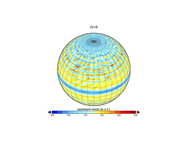
(a)

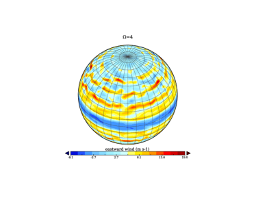
(b)

(d)

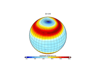
(f)

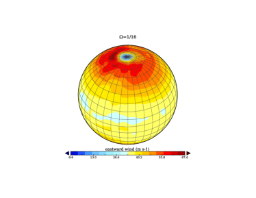
(h)

Figure 3: Snapshots of upper level (200 hPa) zonal wind, projected onto a spherical surface at $\Omega^{\ast}=8$ [(a)], 4 [(b)], 2 [(c)], 1 [(d)], 1/2 [(e)], 1/4 [(f)], 1/8 [(g)] and 1/16 [(h)], illustrating the basic organization of winds across the planet.

(a)                                                                          (b)

(c)                                                                          (d)

(e)                                                                          (f)

(g)                                                                          (h)

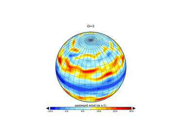
(c)

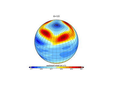
(e)

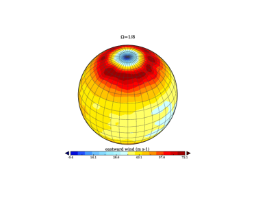
(g)

3.2 Cyclostrophic, super-rotating flow

This regime is found under conditions in which the planet rotates much more slowly than the Earth. Due to the weakness of the Coriolis force on these slow rotators, the major force balance accounting for the large-scale atmospheric motion is between the pressure gradient and the centrifugal “force”, known as cyclostrophic balance (see Holton (1992)). Another distinctive feature of this kind of circulation is that there is typically a very strong prograde zonal wind over the equatorial regions, in contrast to the retrograde wind more typically seen in Earth’s tropical atmosphere, a phenomenon known as equatorial super-rotation (e.g. see Read (1986); Read and Lebonnois (2018)). These features are apparent in the snapshots of zonal wind illustrated in Fig. 3b(f)-(h). A cross-section of the zonal mean zonal wind averaged over the last 360 model days for slowly rotating planets can be seen in Figure 4(n)-(p), which show substantial eastward (prograde) wind in the upper atmosphere over the equator. The extratropical jet streams, which are usually located in mid-latitude or subtropics in Earth’s atmosphere, are pushed further polewards due to the expanded Hadley cells under weak rotational constraints (see Section 4.1 below).

3.3 Regular baroclinic wave flow

For planets with an intermediate thermal Rossby number (larger than Earth’s, but smaller than those of Venus and Titan), planetary scale baroclinic waves are found to occur at mid-latitudes but tend to be very regular and coherent in both their spatial structure and in their time dependence. A perspective view of the upper level $\overline{u}$ field is shown in Fig. 3b(e). This simulation has a roughly similar thermal Rossby number to that of Mars, and a regular baroclinic wave with a dominant mode of either wavenumber-4 or wavenumber-3 is found at the 500 hPa level (see Section 5 for further discussion).

3.4 Irregular baroclinic wave flow

This is the circulation regime that resembles the Earth’s atmospheric circulation more closely than other regimes reported here. It is characterised by spatially and temporally irregular baroclinic waves with mixed wavenumbers and aperiodic (probably chaotic) time-dependence. This regime typically exhibits a single, meandering jet stream in each hemisphere, in which the shape of the wavy structure changes irregularly with time in terms of both phase and amplitude. The flow in Fig. 3b(d) is not dominated by a single zonal wavenumber mode but by a range of wavenumbers from $\sim 5-8$ which fluctuates continuously (see also Fig. 6 below).

3.5 Multiple zonal jet flow

For planets with much smaller thermal Rossby number than the Earth ($\mathcal{R}o_{T}<10^{-2}$), the development of geostrophic turbulence in the presence of a strong $\beta$-effect and weak friction leads to the formation and maintenance of a flow pattern dominated by multiple eddy-driven zonal jets. Characterised by multiple eddy-driven jets over the extratropical regions, flows in this region of parameter space develop strongly zonal structures at planetary scale, as shown in Fig. 3b(a)-(c), in contrast to the rather more obviously meandering wavy structures of other non-axisymmetric regimes. It is notable that gas giant planets in the Solar System (Jupiter, Saturn, Uranus and Neptune) all exhibit a set of strong, parallel, nearly rectilinear zonal jets (Showman et al. (2010)), as reflected in their banded appearances. The experiment with $\Omega^{\ast}=8$ has a somewhat similar value of $\mathcal{R}o_{T}$ to Jupiter and Saturn (as can be appreciated from Fig. 2). Recent studies suggest that such banded zonal jets can also be found in the Earth’s oceans (for example, as found in the eddy-resolving ocean model simulations of the North Pacific Ocean, e.g. see Galperin et al. (2004)), but the resulting jets are much weaker and more strongly meandering.

The diversity of circulation regimes identified in this regime diagram suggests a number of fundamental questions regarding the general circulation of planetary atmospheres: What determines the preferred eddy scales in a planetary atmosphere? How does the planetary rotation rate affect the meridional heat transport? What causes and maintains the equatorial superrotation when rotation rate is low? What determines the selection of wavenumbers in steady baroclinic waves? Why do eddies organise themselves into jets and what insights can be obtained on the jet formation mechanism from modern theories of geostrophic turbulence? With these questions in mind we will investigate the structures and trends of the circulation regimes in the following sections.

4 Phenomenology

4.1 Zonal mean circulation

Since the incoming solar radiation, which serves as the ultimate energy source of the atmospheric circulation, generally varies most in the meridional direction, the large-scale motion of the atmosphere has greater variations in the meridional direction than in the zonal direction, especially when averaging over a long time period compared to other dynamical timescales. Thus, analysis of zonal averages of the meteorological variables takes a particularly significant role in the study of atmospheric general circulation. The zonal mean absolute and potential temperature ($T$ and $\theta$ - left column) and zonal wind ($\overline{u}$) contours (right column) for different $\Omega$ and $\Delta T_{h}=60\ \text{K}$ are shown in Fig. 4, with the meridional mass streamfunction superimposed on $\overline{u}$ using colour shading.

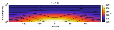
(a)

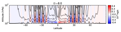
(b)

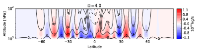
(d)

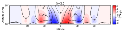
(f)

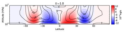
(h)

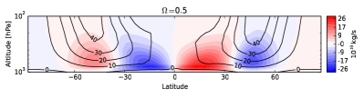
(j)

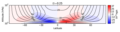
(l)

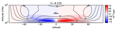
(n)

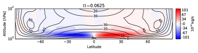
(p)

(a)                                                                          (i)

(b)                                                                          (j)

(c)                                                                          (k)

(d)                                                                          (l)

(e)                                                                          (m)

(f)                                                                          (n)

(g)                                                                          (o)

(h)                                                                          (p)

(c)

(e)

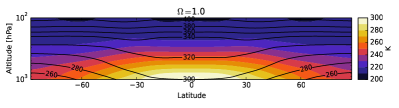
(g)

(i)

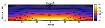
(k)

(m)

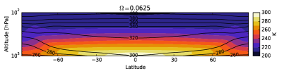
(o)

Figure 4: Zonal mean fields of temperature (absolute, $T$, and potential, $\theta$) [(a) - (h)] and zonal wind and meridional streamfunction [(i) - (p)] for $\Omega^{\ast}=8$ [(a) & (i)], 4 [(b) & (j)], 2 [(c) & (k)], 1 [(d) & (l)], 1/2 [(e) & (m)], 1/4 [((f) & (n)], 1/8 [(g) & (o)] and 1/16 [(h) & (p)]. Shading indicates absolute temperature in (a) - (h) and meridional streamfunction in (i) - (p), while contours indicate potential temperature [(a) - (h)] and zonal velocity [(i) - (p)].

The fastest rotating experiments ($\Omega^{\ast}>1$) are characterised by multiple parallel extratropical jet streams. The generation and maintenance of these jets through upscale energy transfers, which are characteristic of highly anisotropic geostrophic turbulence, will be discussed in a further companion paper (Read et al., 2017). At this stage we focus on describing the change of global structures—the increase of the number of jets with $\Omega$ — and identifying the key lengthscales that determine the global structure in the zonal mean. The characteristic latitudinal range of anisotropy associated with the latitudinal variation of Coriolis parameter $f$ can be estimated by the Rhines scale (Rhines, 1975):

$$L_{R}=\Big{(}\dfrac{2U}{\beta}\Big{)}^{1/2},$$ (12)

in which $U$ is a characteristic horizontal wind speed. The original argument in Rhines (1975) used $U_{\text{rms}}$, which is the root mean square velocity (often taken to be the rms eddy velocity). Other work, however, has suggested that the rms zonal mean velocity, $\overline{U}$, is more appropriate in defining $L_{R}$ (e.g. Dunkerton and Scott, 2008). Here, we apply the thermal wind relationship to the zonal mean temperature field to estimate $\overline{U}$ (e.g. see Read (2011)) which leads to:

$$L_{R1}\simeq\Big{(}\dfrac{R\Delta\theta_{h}}{\Omega^{2}}\Big{)}^{1/2}=a(\mathcal{R}o_{T})^{1/2}.$$ (13)

The number of eddy-driven jets expected on a planet can then be estimated as

$$N_{J}\simeq\dfrac{\pi a}{2}\dfrac{1}{2\pi L_{R}}=\dfrac{a}{4L_{R}},$$ (14)

which leads to an estimate based on the zonal mean thermal wind of

$$N_{J1}\simeq\dfrac{1}{4\mathcal{R}o_{T}^{1/2}}.$$ (15)

This leads to an estimate that is somewhat similar to the formulation suggested by Lee (2005) ($N_{J}\propto(a/\Delta\theta_{h})^{1/2}$) though with a different dependence on $a$.

Table 1 shows the values of various key dimensionless parameters for the main series of runs discussed here, including the number of jets on a planet surface predicted by Eq. (14) and (15). For experiments with very slow rotation rates ($\Omega^{\ast}<1/4$), $N_{J1}$ is smaller than $1$. This means that the picture of an eddy-driven jet emerging through an inverse energy cascade in the framework of geostrophic turbulence is no longer valid since the Rhines wavelength, $2\pi L_{R1}$ in this case, exceeds the size of the planetary domain. The jets observed in these slowly rotating simulation experiments are primarily due to the quasi-conservation of angular momentum within the upper branch of the extended thermally-direct Hadley cell. At $\Omega^{\ast}=1$, the predicted number of jets is $1.16$, which approximately corresponds to the regime of two prograde jet per hemisphere. For experiments with faster rotation rates ($\Omega^{\ast}>1$), Eq. (15) predicts up to $14$ jets for $\Omega^{\ast}=8$. This is broadly consistent with the zonal wind map shown in Fig. 4 where at least 8 distinct eastward jets can be located in each hemisphere. The multiple jets for $\Omega^{\ast}=2$ and 4, however, were seen to drift slowly polewards, much as found by Chemke and Kaspi (2015b), although this was less evident for the $\Omega^{\ast}=8$ case for which the spatial resolution may have been insufficient to reveal this behaviour clearly.

$\Omega^{\ast}$	$\mathcal{R}o_{T}$	$\mathcal{T}a_{f}$	$\mathcal{T}a_{R}$	$N_{J1}$	$N_{J2}$
$1/16$	20.5	238	1.71 $\times 10^{5}$	0.08	0.49
$1/8$	5.14	3.80 $\times 10^{3}$	2.73 $\times 10^{6}$	0.14	0.77
$1/4$	1.28	6.09 $\times 10^{4}$	4.67 $\times 10^{7}$	0.29	0.96
$1/2$	0.32	9.74 $\times 10^{5}$	6.98 $\times 10^{8}$	0.58	1.06
$1$	0.08	1.56 $\times 10^{7}$	1.12 $\times 10^{10}$	1.1	1.25
$2$	0.02	2.49 $\times 10^{8}$	1.79 $\times 10^{11}$	2.2	3.1
$4$	0.005	3.99 $\times 10^{9}$	2.86 $\times 10^{12}$	3.9	6.1
$8$	0.0013	6.38 $\times 10^{10}$	4.58 $\times 10^{13}$	7.1	13.9

Table 1: Key dimensionless parameters for the baseline set of numerical simulations with $\Delta\theta_{h}=60\text{K}$, $\tau_{ft}=5$ Earth days and $\tau_{R}=25.9$ Earth days, as defined by Equations (8), (10), (14), (15) and (21).

As we can see from Figs. 4, the subtropical jet stream moves to higher latitude as the rotation rate decreases, which is consistent with the prediction from the quasi-inviscid axisymmetric Hadley cell theory (see Held and Hou (1980); Caballero et al. (2008)). The intensity of the jet stream grows stronger as the rotation rate decreases until $\Omega^{\ast}=1/8$. For the $\Omega^{\ast}=1/16$ run, the extratropical jet ($\sim 60\ \text{m s}^{-1}$) is actually weaker than that in the $\Omega^{\ast}=1/8$ run ($\sim 70\ \text{m s}^{-1}$). In principle, there are two competing factors determining the intensity of the extratropical jet stream as the rotation rate decreases. The jet stream reaches a higher latitude, thus gaining more angular velocity for a given angular momentum than at lower latitudes. On the other hand, the reduction in rotation rate actually decreases the angular momentum of the whole planet, thus reducing the angular momentum obtained by the poleward moving jet stream. For the runs from $\Omega^{\ast}=1$ to $\Omega^{\ast}=1/8$, the first factor dominates and the jet intensity gets stronger for smaller rotation rates. But for the $\Omega^{\ast}=1/16$ run, the latter factor begins to dominate and the angular momentum of the background planetary rotation reduces sufficiently to offset the angular momentum gain caused by the poleward motion of the jet stream (similar results were found by Navarra and Boccaletti (2002)).

This poleward movement of the subtropical jet stream is a clear indication of the expansion of the Hadley cell in each hemisphere as the rotation rate decreases. This can be evaluated by the zonal mean meridional mass streamfunction, defined in the pressure coordinate system as (see Peixoto and Oort (1992)):

$$\Psi=\frac{2\pi a}{g}\cos{\phi}\int_{0}^{P}dp^{\prime}[\overline{v}],$$

where $a$ is the planetary radius, $[\overline{v}]$ the zonal and temporal mean meridional velocity, $\phi$ the latitude and $P$ the surface atmospheric pressure.

As anticipated (see Fig. 4(right column)), there are basically three cells in each hemisphere for the terrestrial rotation rate ($\Omega^{\ast}=1$). The positive values of $\Psi$ represent clockwise flow and the negative values represent counter-clockwise flow, while the magnitude reflects the strength of the overturning. The poleward edge of the overturning Hadley circulation can be estimated by the latitude of the boundary between the tropical cell and the adjacent mid-latitude cell. In the $\Omega^{\ast}=1$ case, the extent of the Hadley cell in each hemisphere is roughly $30^{\circ}$, which is consistent with the observed value for the Earth. As the rotation rate decreases, the overturning Hadley cell expands and intensifies, much as predicted in the previously cited Held and Hou (1980) and Caballero et al. (2008) models. In fact, at the lowest rotation rate, $\Omega^{\ast}=1/16$, only one strong hemispherically-dominating Hadley cell is found in each hemisphere while the other two cells at mid- and high-latitudes disappear. Within the Hadley cell, baroclinicity (associated with the meridional slope of isentropic surfaces, and hence the horizontal temperature difference in the meridional direction) is considerably weaker compared to that in the extratropical baroclinic eddy zones. This feature is reflected in the zonal mean temperature cross-sections in Fig. 4(left column).

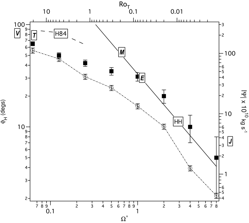
Figure 5: Variations of (a) the strength of the main Hadley streamfunction (shown as open circles) and (b) the width of the main Hadley circulation as a function of $\Omega^{\ast}$ and $\mathcal{R}o_{T}$ (shown as solid squares), estimated from the latitudinal width of the mass streamfunction contour at 10% of the peak value in mid-troposphere in each case. The solid line shows the expected variation predicted by the simple model of Held and Hou (1980), scaled by $\pi/2a$, while the dashed line shows the expected variation in the slowly rotating limit by Hou (1984). The observed or modelled widths of the Hadley cells on Earth, Mars, Venus, Titan and Jupiter are indicated by their initial letters (see text).

Figure 5 shows the variation of the actual width of the thermally-direct Hadley cell at each value of $\Omega^{\ast}$ and $\mathcal{R}o_{T}$, estimated by the angular width of the mass streamfunction contour at 10% of the peak value (shown as filled squares). This may be compared with the latitudinal width

$$Y_{HH}\simeq a\left(\dfrac{5}{3}\mathcal{R}o_{T}\right)^{1/2},$$ (16)

predicted by the simple models of Held and Hou (1980) and Caballero et al. (2008) (which differs from Held and Hou (1980) only by a factor O(1) that depends on radiative-convective factors). The length scale $\pi Y_{HH}/2a$ is shown for reference as a solid line in Fig. 5. The Hadley cell width in the GCM simulations is seen to scale quite closely with the Held-Hou model for $\Omega^{\ast}\geq 1$, but then increases much more slowly with increasing $\mathcal{R}o_{T}$ as it approaches the radius of the planet itself. At the lowest values of $\Omega^{\ast}$, the width tends towards 80-90^∘, much as predicted in the extension of the Held-Hou model by Hou (1984).

Estimates of the Hadley cell widths for Earth, Mars, Titan, Venus and Jupiter are also shown for comparison, indicated by their initial letters. The widths for Earth and Mars were estimated following Read (2011) from the ERA40 reanalysis (Uppala et al., 2005) and the annual zonal mean results of Read and Lewis (2004) respectively. Widths for Venus and Titan were estimated respectively from the GCM results of Lebonnois et al. (2010) and Lebonnois et al. (2012), while for Jupiter we show the approximate width of the equatorial zone. These are largely consistent with the simple GCM and Held-Hou results except for Mars, whose annual mean Hadley circulation is rather broader than the Held-Hou results would suggest. However, for much of the Martian year the meridional circulation is dominated by a single large, cross-equatorial cell which extends over a wider range of latitude than at equinoxes.

The strength of the meridional Hadley circulation in the simulations is also shown in Fig. 5 as a function of $\Omega^{\ast}$ and $\mathcal{R}o_{T}$. This indicates a reduction in the strength of the circulation by a factor of $\sim 250$ between $\Omega^{\ast}=1/16$ and 8. $|\Psi|$ follows a scaling close to $\mathcal{R}o_{T}^{2/5}$ for $\Omega^{\ast}\leq 2$ which steepens to a scaling closer to $\mathcal{R}o_{T}^{3/5}$ for $\Omega^{\ast}\geq 2$. This absolute magnitude of the mass streamfunction is of the same order as that found by Kaspi and Showman (2015), although the strength of their Hadley circulations decreased somewhat less rapidly with $\Omega^{\ast}$. Both models show a much less steep decline in $|\Psi|$ with $\mathcal{R}o_{T}$ than the $\phi_{H}^{3}\sim\mathcal{R}o_{T}^{3/2}$ indicated by Caballero et al. (2008).

At higher rotation rates, the three-cell meridional circulation shrinks towards the equator and additional cells appear at high latitudes. These additional cells are essentially eddy-driven and are aligned with the positions of the multiple eddy-driven zonal jets that appear at middle and high latitudes, though retaining a thermally-direct circulation close to the equator itself in each hemisphere.

4.2 Non-axisymmetric features — eddies/waves

For rapidly rotating planets like the Earth and Mars, the maintenance of the general circulation and the transport of heat and momentum depend significantly on the interactions between transient eddies and the mean flow. In the absence of eddies, the atmosphere of the mid- and high-latitudes would reach a state of radiative equilibrium, which is characterised by larger meridional temperature contrasts than we observe here. Thermal winds induced by such strong temperature gradients would then lead to wind shears in the vertical direction which are baroclinically unstable. The baroclinic eddy transport of heat considerably reduces the equator-to-pole temperature difference from that predicted by radiative equilibrium. In this section, we will investigate the general trends of eddy activity with planetary rotation rate.

Fig. 6 shows the zonal wavenumber amplitude spectra of geopotential height at the 500 hPa level as a function of latitude from experiments with various rotation rates. As the rotation rate decreases, the eddies become more and more confined to smaller wavenumbers, eventually converging towards $m=1$ at the lowest values of $\Omega^{\ast}$. This is consistent with the trend with rotation of the energy-containing scales, as represented by the Rossby deformation radius and the Rhines scale. At high rotation rates (e.g. $\Omega^{\ast}=4$ and $8$), noticeable parallel banded structures can be seen in the extratropical latitudes, indicating the existence of multiple baroclinic zones, as would be expected if the characteristic eddy length scale is significantly smaller than the planetary domain. The zonal wavenumber spectra themselves at these high rotation rates also peak at much higher wavenumbers. The Fourier amplitude is smaller for high rotation rate spectra as a result of the decreased eddy length scale, which leads to a smaller intensity of perturbations. The maximum strength of eddy activity is found at higher latitudes for experiments with lower rotation rates, which is again consistent with the trend that Hadley cells tend to expand as $\Omega^{\ast}$ reduces, pushing extratropical jets (along with associated eddies) polewards as the rotation rate decreases.

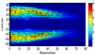
(a)

(b)

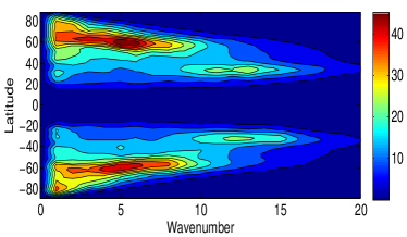
(c)

(d)

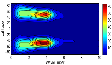
(e)

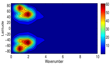
(f)

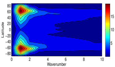
(g)

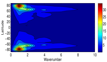
(h)

Figure 6: Fourier amplitude maps of the zonal wavenumber spectra of geopotential height at 500 hPa from experiments at various rotation rates.: (a) $\Omega^{\ast}=8$, (b) $\Omega^{\ast}=4$, (c) $\Omega^{\ast}=2$, (d) $\Omega^{\ast}=1$, (e) $\Omega^{\ast}=1/2$, (f) $\Omega^{\ast}=1/4$, (g) $\Omega^{\ast}=1/8$, $\Omega^{\ast}=1/16$. Spectra are averaged over one model year. Unit: geopotential metres.

4.3 Characteristic scales of eddies

The preferred scale of non-axisymmetric eddies can be defined as the energy containing wavenumber $n_{e}$, based on the global barotropic eddy kinetic energy spectrum of the atmosphere (Schneider and Walker (2006)):

$$n_{e}(n_{e}+1)=\displaystyle\frac{\sum\limits_{n}E_{n}}{\sum\limits_{n}\big{[}n(n+1)\big{]}^{-1}E_{n}},$$ (17)

in which $E_{n}$ is the barotropic eddy kinetic energy density at spherical harmonic wavenumber $n$, computed following Koshyk et al. (1999) as a vertical, mass-weighted average for the components with non-zero zonal wavenumber.

Linear theories of baroclinic instability (Eady (1949), Charney (1947)) predict the characteristic eddy length scale to be the wavelength of the fastest growing unstable mode, which can be estimated by the first baroclinic Rossby deformation radius. But if nonlinear eddy-eddy interactions and the consequential inverse energy cascade are taken into account, the characteristic eddy length scale will be the scale at which the inverse energy cascade is inhibited. This is shown to be characterised by the so-called Rhines scale (Rhines (1975)), or the size of the whole domain if the Rhines scale exceeds the bound of the domain. It is therefore interesting to see how Rossby deformation and Rhines scales vary with the rotation rate in our experiments and whether there is a scale separation due to the potential cascade of kinetic energy.

Following Schneider and Walker (2006), the Rossby deformation radius is calculated as:

$$L_{D}=c_{D}\frac{NH}{f_{0}}=c_{D}\frac{N_{p}\Delta p}{f_{0}},$$ (18)

where $N_{p}^{2}=-(\overline{\rho}_{s}\overline{\theta}_{s})^{-1}\overline{\partial_{p}\theta}^{s}$ is the static stability measure, $\Delta p$ the pressure difference between tropopause and ground level, and $\rho_{s}$ is the atmospheric density at the surface. Since it is the extratropical (baroclinic) Rossby deformation radius that is interesting to compare with, this deformation radius is averaged within the baroclinic zone whose boundaries are defined as the outermost latitudes at which the meridional heat flux $\overline{v^{\prime}\theta^{\prime}}\cos{\phi}$ at the near surface level ($800\ \text{mb}$) exceeds $30\%$ of its maximum value. The empirical constant $c_{D}$ is chosen to be $1.35$ following Schneider and Walker (2006).

The Rhines scale is calculated as:

$$L_{R2}=\sqrt{2U/\beta}=\frac{\text{EKE}_{\text{bt}}^{1/4}}{\beta^{1/2}},$$ (19)

where $U$ is now the rms flow speed, and $\text{EKE}_{\text{bt}}$ is the barotropic eddy kinetic energy density (see Section 4.3 above). The corresponding Rossby and Rhines wavenumbers can be defined respectively as:

$$n_{D}(n_{D}+1)=a^{2}/L_{D}^{2},\ n_{R}(n_{R}+1)=a^{2}/L_{R}^{2}.$$ (20)

This also leads to an alternative estimate of the number of jets, based on Eq (14) using $L_{R2}$ as defined in Eq (19), which equates to

$$N_{J2}=\dfrac{a}{4L_{R2}}=\dfrac{n_{R}}{4}.$$ (21)

This estimate is also shown in Table 1 and is seen to differ from $N_{J1}$ by a factor $\sim 2$. $N_{J2}$ is generally larger than $N_{J1}$ and becomes greater than unity around $\Omega^{\ast}=1/2$, but otherwise follows a similar trend to $N_{J1}$, at least for this set of simulations. $N_{J1}$ appears to provide a more realistic estimate of the number of jets in each hemisphere for $\Omega^{\ast}\geq 1$, however, similar to Lee (2005) although the latter is based on somewhat different physical assumptions.

Fig. 7 show the comparison of Rossby wavenumber $n_{D}$, Rhines wavenumber $n_{R}$ and the energy-containing wavenumber $n_{e}$, as $\Omega^{\ast}$ is varied. It can be seen that these three wavenumbers are generally quite similar to each other in this set of simulations, though with $L_{R}>L_{D}$. This agrees with the results of Schneider and Walker (2006) in which they found that their simulated atmospheric macroturbulence tended to self-organise into a state of weak nonlinear eddy-eddy interactions with supercriticality $S_{c}\sim 1$, where supercriticality, $S_{c}$, is defined as

$$S_{c}=\frac{f}{\beta H}\frac{\partial_{y}\overline{\theta}}{\partial_{z}\overline{\theta}},$$ (22)

a nondimensional measure of either the slope of the isentropes near the ground (see Schneider and Walker, 2006) or the (squared) ratio between the Rossby deformation scale and the Rhines scale (e.g. see Held and Larichev, 1996). As the Rhines wavenumber is close to the baroclinic Rossby wavenumber, this suggests that the inertial range for an inverse energy cascade via eddy-eddy interactions is likely to be largely inhibited, which is consistent with the fact that no well-defined $-5/3$ slope in the barotropic eddy kinetic energy spectrum is observed in our experiments (see Read et al. (2017) for more discussion) although this may be an oversimplification given the different dependence of the Rhines and Rossby lengthscales on latitude (see below). According to Schneider (2004) and Schneider and Walker (2006), such self-organisation is achieved through the adjustment of the extratropical thermal stratification by baroclinic eddies. This mode of equilibration is not allowed in the traditional quasi-geostrophic theories where the thermal stratification is taken to be fixed. This is consistent with the historical success of linear or weakly nonlinear theories of dynamical meteorology for extratropical regions. It should be mentioned, however, that some recent studies find that, under some circumstances, an Earth-like atmosphere or ocean can adjust into states with a supercriticality very different from 1 if the external forcings and planetary parameters are varied sufficiently (e.g. see Zurita-Gotor (2008), Jansen and Ferrari (2012)). Thus, the results presented here and in Schneider and Walker (2006) are valid probably only within a subset of the parameter space.

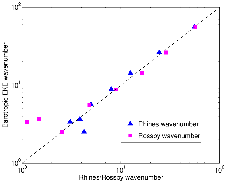
Figure 7: Energy-containing wavenumber of barotropic eddy kinetic energy ($n_{e}$) vs Rossby wavenumber ($n_{D}$) and Rhines wavenumber ($n_{R}$) for experiments with $\Omega^{\ast}=1/16,1/8,1/4,1/2,1,2,4,8$. $n_{e}=n_{D}$ or $n_{R}$ along the dashed line.

Because of the different dependences of $L_{D}$ and $L_{R}$ on latitude, the local supercriticality, $S_{c}(\phi)$, is also a strong function of latitude. This was explored recently by Chemke and Kaspi (2015a), who noted that inverse energy cascades could be found over certain latitude ranges, depending upon planetary size and rotation rate. Figure 8 shows the variation with latitude of the supercritical latitude, $\phi_{S}$, defined as the latitude at which the (latitude-dependent) Rhines and Rossby deformation length scales (determined according to Eqs (19) and (18)) become equal in magnitude. This clearly shows a transition around $\Omega^{\ast}=1$ between the slowly rotating regime, where $\phi_{S}\rightarrow 90^{\circ}$, and more rapidly rotating regimes where $\phi_{S}$ takes an intermediate value between $\sim 40^{\circ}$ and 20^∘. Polewards of $\phi_{S}$, we find that $L_{R}>L_{D}$, allowing for the possibility of an inverse cascade of kinetic energy from a baroclinic injection scale around $L_{D}$ towards $L_{R}$. Equatorwards of $\phi_{S}$, however, $L_{R}<L_{D}$, suggesting that only forward transfers of KE are likely to occur.

Figure 8: Variation with $|\Omega|^{\ast}$ and $\mathcal{R}o_{T}$ of the supercritical latitude, $\phi_{S}$, defined as the latitude where the Rhines and Rossby deformation lengthscales are equal.

This suggestion is further confirmed, at least for cases for which $\Omega^{\ast}\geq 1$, from a comparison between the Rhines and Rossby lengthscales (computed in the same way as by Chemke and Kaspi (2015a)) on the one hand and the zonal jet wavelength and kinetic energy weighted lengthscales on the other. Two examples of such a comparison for $\Omega^{\ast}=4$ and 8 are shown in Figure 9. The jet wavelength, $L_{Z}$, is shown as individual dots, representing the computed distance between successive eastward or westward extrema in $\overline{u}$, while the most energetic eddy lengthscale, $L_{e}$, is computed in a similar way to Eq (17) for $n_{e}$ but for zonal wavenumber $m$ only at each latitude point, thus,

$$L_{e}(\phi)=2\pi\cos\phi\left(\dfrac{\sum\limits_{m}E_{K}^{m}(\phi)/m^{2}}{\sum\limits_{m}E_{K}^{m}(\phi)}\right)^{1/2},$$ (23)

where $E_{K}^{m}(\phi)$ is the eddy kinetic energy spectral density at zonal wavenumber $m$ and latitude $\phi$.

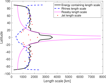
(a)

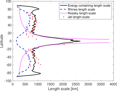
(b)

(a)                                                                          (b)

Figure 9: Profiles showing the latitudinal variation of Rossby deformation and Rhines lengthscales, $L_{D}(\phi)$ and $L_{R}(phi)$, compared with the meridional wavelength of the multiple, eddy-driven zonal jets, $L_{Z}$, and the kinetic energy containing lengthscale, for (a) $\Omega^{\ast}=4$ and (b) $\Omega^{\ast}=8$. $L_{e}$. $L_{D}$ is shown as a dotted line while $L_{R}$ is shown as a dashed line. $L_{e}$ is denoted by the solid line and the zonal jet wavelength, $L_{Z}$, is indicated by individual dots.

Fig. 9(a) clearly shows both $L_{Z}$ and $L_{e}$ aligning closely with $L_{R}$ for $\phi>\phi_{S}$ (where $\phi_{S}\simeq 25^{\circ}$) for $\Omega^{\ast}=4$, but with both $L_{Z}$ and $L_{e}$ diverging from $L_{R}$ for $\phi<\phi_{S}$ and following a trend that appears to parallel the behaviour of $L_{D}$. This behaviour is similar to what e.g. Chai and Vallis (2014) and Chemke and Kaspi (2015a) found in their models, using different methods of radiative forcing, and suggests an important role for eddy-eddy interactions in cascading EKE to larger scales than $L_{D}$. A broadly similar trend is also found for $\Omega^{\ast}=1$ and 2 (not shown), and for $\Omega^{\ast}=8$ (see Fig. 9(b)), although in this case $L_{Z}\simeq L_{e}>L_{R}$. This may result from the limited spatial resolution in the $\Omega^{\ast}=8$ case although this should be investigated more closely in future work. At much lower rotation rates, $L_{Z}$ becomes ill defined (since there are no longer multiple eddy-driven jets) and $L_{e}$ roughly follows the trend of $L_{R}$, though this apparent correlation may be coincidental. Thus, the detailed links between $L_{e}$, $L_{R}$ and $L_{D}$ are more subtle and dependent on latitude and other parameters than the global behaviour shown in Fig. 7 might suggest.

4.4 Heat transfer

The efficiency by which heat is transferred from the warm tropical regions of an Earth-like planetary atmosphere to the cooler mid- and high-latitudes is an important characteristic of the global atmospheric circulation. It largely determines how the climate varies from place to place, and in particular sets the mean temperature contrast between the tropics and polar regions. For the Earth, how this efficiency depends upon key parameters relating to the thermodynamic driving of the atmospheric circulation is important for understanding and quantifying the response of the climate system e.g. to changing amounts of greenhouse gases in the atmosphere. For other planets, heat transfer efficiency may affect their potential habitability and long term evolution, while also strongly influencing the strength of the meridional and zonal winds. The way in which horizontal heat transfer is partitioned between meridional overturning and eddies in the Earth’s atmosphere has been well documented in both observations and numerical simulations for many years (e.g. Peixóto and Oort, 1974; James, 1995). But for other planets in the Solar System, for which detailed observations are much sparser than for Earth, this remains a challenging question. Although latent heat plays an important role in the Earth’s atmosphere, for a dry atmosphere (such as that of Mars or Venus) the primary form of heat energy is as sensible heat or dry static energy. The intensity by which heat energy is transferred within such a dry atmosphere depends strongly on the dynamical regime.

From a cursory examination of the zonal mean temperature fields (see Fig. 4), the equator-pole temperature gradient becomes much smaller as the rotation rate decreases. This is especially prominent at the middle and high levels of the atmosphere, where the isotherms become almost horizontal at low rotation rates. As also discussed e.g. by (Kaspi and Showman, 2015), this tendency at low rotation rates is due to the strong and extensive overturning Hadley cell in each hemisphere, which is highly efficient in smoothing out the horizontal temperature inhomogeneity. At higher rotation rates, however, baroclinic eddies likely play a more important role and the meridional temperature gradient is found to steepen. For $\Omega^{\ast}>1$ the meridional temperature variation is seen to show staircase-like features, indicating the existence of multiple, zonally-parallel baroclinic zones and belts, at least superficially resembling the banded structure of the Jovian atmosphere. This is particularly apparent in the PUMA-S simulations for $\Omega^{\ast}=2$ and 4, though with some hints of such effects even at Earth-like rotation rates.

The time-averaged meridional eddy sensible heat flux, which can be formulated as $[\overline{v^{\ast}T^{\ast}}]$, provides a measure of the intensity of meridional heat transfer by eddies. All of the PUMA-S simulations show that the atmosphere (especially at the lower levels) is dominated by poleward eddy heat transport. The strength of eddy heat flux reaches its maximum in the extratropical baroclinic regions, with multiple local maxima in latitude for experiments at the higher rotation rate (e.g. $\Omega^{\ast}=2,4,8$), which is consistent with the existence of multiple baroclinic zones obtained in these experiments.

$\overline{[v^{\ast}T^{\ast}]}$ is significant only in the extratropical regions (where the atmosphere is dominated by eddies and waves rather than quasi-axisymmetric circulation cells), and so the simple areal and mass-weighted average of $[v^{\ast}T^{\ast}]$ over the whole globe is not particularly informative. A clearer measure is provided by the peak value of the time-averaged heat transport, integrated (and mass-weighted) over the entire meridional plane (cf Kaspi and Showman, 2015, for example). The sensitivity of the peak, vertically integrated meridional eddy heat flux $\int\rho c_{p}\overline{[v^{\ast}T^{\ast}]}dp/g$ to changes of rotation rates is shown in Fig. 10(a) (crosses and dashed lines), based on experiments with $\Delta T_{EP}=60K$ at various rotation rates, together with corresponding values of the peak zonal mean contribution $\int\rho c_{p}\overline{[v][T^{\prime}]}dp/g$ (triangles and dotted lines) and the sum of these representing the total (squares and solid lines). From these variations, it can be seen that, as rotation rate decreases from $\Omega^{\ast}=8$, the strength of the meridional eddy heat flux increases monotonically until it reaches its maximum at $\Omega^{\ast}\simeq 1/2$, indicating the prominence of baroclinic eddies at this rotation rate. As the rotation rate decreases further below $\Omega^{\ast}=1/2$, the meridional eddy heat flux is seen to become less intense as the global circulation becomes more and more dominated by direct meridional overturning Hadley cells, which extend far into the high-latitudes at the slowest rotation rates. The strength of the Hadley heat transport is reflected in $\int\rho c_{p}\overline{[v][T^{\prime}]}dp/g$, which shows a monotonic decrease with $\Omega^{\ast}$ but evidently dominates the total heat transport at low rotation rates for which $\mathcal{R}o_{T}\gtrsim 1$.

Variations in total heat transport (both meridional and vertical) lead to changes in both the equator-pole temperature contrast and the static stability, which also impacts upon the mean slope of the isotherms and isentropes within the simulated circulation. This suggests that the mean slope of the potential temperature isotherms actually reflects a measure of the total efficiency of heat transport (both horizontal and vertical) within the atmosphere. However, the slope angle by itself is not enough to quantify this efficiency since, even in pure radiative equilibrium, the isotherms would exhibit a non-zero slope because of the differential radiative heating with latitude. A more meaningful nondimensional measure of the atmospheric heat transport efficiency can therefore be defined with respect to the radiative-convective equilibrium state towards which the atmosphere tries to relax as the following:

$$\eta_{h}=\frac{\langle\partial_{y}\theta_{e}/\partial_{z}\theta_{e}\rangle}{\langle\overline{\partial_{y}\theta/\partial_{z}\theta}\rangle},$$ (24)

where $\theta$ is the potential temperature observed in the GCM results, $\theta_{e}$ the prescribed (equilibrium) potential temperature used by the Newtonian relaxation scheme and $\partial_{z},\ \partial_{y}$ the vertical and meridional derivatives respectively. $\eta_{h}$ thus represents the mean ratio of the meridional slope of the isotherms relative to that of the restoration state (i.e. representing the ultimate baroclinicity of the atmosphere). The more efficient the dynamic heat transfer, the lower the realised isentrope slope. Higher values of $\eta_{h}$ therefore correspond to more efficient atmospheric heat transfer. This diagnostic thus provides a nondimensional measure of the efficiency of total dynamic heat transport, which redistributes heat, not only meridionally but also vertically. It should also be noted, however, that $\eta_{h}$ measures the total heat transport, by both the meridional mean circulation (e.g. Hadley cell) and the eddies.

Fig. 10(b) shows the comparison of $\eta_{h}$, based on the same simulations as in Fig. 10(a). It can be seen that, at the faster rotation rates, the redistribution of heat by dynamical processes tends to be inhibited, which includes both direct meridional overturning circulations (Hadley cells) as well as non-axisymmetric waves and eddies. Note that the downward trend is almost arrested around $\Omega^{\ast}\simeq 1/4-1$, which corresponds to where $\mathcal{R}o_{T}\simeq 1$. This indicates that in this parameter regime the eddy heat transport tends to compensate significantly for the decreasing efficiency of Hadley cell heat transport, thus preventing the total heat transport from collapsing as rotation rate increases. This is similar in many respects to the findings of laboratory and numerical annulus experiments, where non-axisymmetric flows are found to sustain stronger levels of total heat transport well into the baroclinically unstable regime than would be sustained by pure axisymmetric flows as the rotation rate increases (Hide and Mason (1975); Read (2003)). This compensating effect persists until the system enters the multiple eddy-driven jet regime, where meridional eddies are no longer able to propagate and transport heat energy uniformly from the tropics to the poles.

(a)

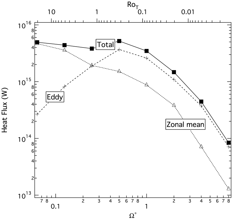
(b)

Figure 10: (a) Variations of peak values of meridional heat transport (in W), shown as total poleward transport (blue squares), zonal mean transport ($\int[\rho c_{p}\overline{v}\overline{T}]dp/g$) and eddy transport ($\int[\rho c_{p}\overline{v^{\ast}T^{\ast}}]dp/g$); (b) ratio of globally mass-weighted average isentropic slope in radiative-convective equilibrium (towards which the model atmosphere relaxes) to the slope obtained in fully active circulations in the latitude-height plane for experiments with different $\Omega^{*}$ (shown as filled triangles connected by solid lines), plotted alongside the variation of mean equator-pole thermal contrast in the mid-troposphere, $\Delta T_{EP}$ (shown as open squares connected by a dotted line).

A related trend is also apparent in the emergent thermal contrast between equator and poles, $\Delta T_{EP}$. This is also illustrated in Fig. 10(b), indicated by the open squares connected by a dotted line, where $\Delta T_{EP}$ is defined as the temperature difference between equatorial and polar latitudes over the pressure range 600 hPa $\geq p\geq$ 400 hPa. This shows a nearly monotonically increasing trend with $\Omega^{\ast}$, though with an apparent pause between $\Omega^{\ast}=0.2$ and 1. Such a pause is also consistent with a degree of baroclinic adjustment close to the onset of dominance of baroclinic instability over barotropic instabilties.

5 The regular baroclinic wave regime

A regular baroclinic wave regime lies in the range $0.1<\mathcal{R}o_{T}<1.5$ within the non-axisymmetric region. Being favoured by intermediate rotation rates and moderate imposed meridional/radial temperature contrasts, it also resembles one of the major flow regimes observed in laboratory rotating annulus experiments (see e.g. Hide and Mason (1975)). Featuring baroclinic waves with one or two dominating wavenumbers and their harmonics, this regime is distinguished from irregular/chaotic baroclinic wave regimes by its highly symmetrical regularity/predictability due to the presence of steady or (quasi-)periodic vacillating waves.

Flows within the regular wave regime with intermediate strengths of frictional and thermal damping are typically characterised by one dominant wavenumber component and its harmonics.Two representative cases with dominant wavenumber 3 or 4 respectively are illustrated in Fig. 11, which shows polar view snapshots of the geopotential height field in two experiments with a rotation rate of $\Omega_{E}/2$ and different values of the frictional and radiative damping parameters.

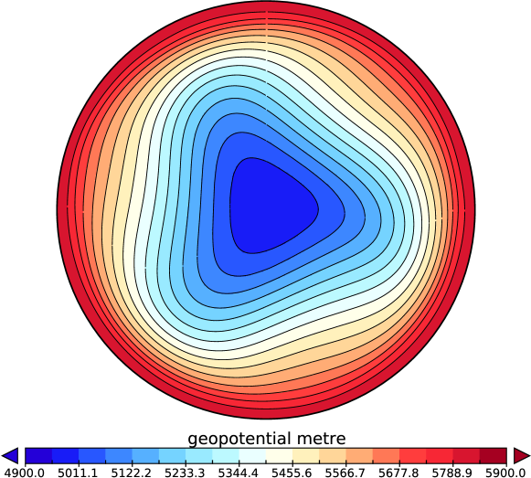
(a)

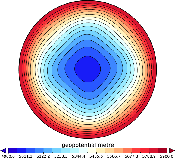
(b)

Figure 11: Snapshots of the geopotential height at the 500 hPa level viewed from the North Pole, showing (a) a wavenumber-3 regime with $\tau_{f}=1.0$ day and $\tau_{R}=7.5$ days, and (b) a wavenumber-4 regime with $\tau_{f}=2.0$ days and $\tau_{R}=1.625$ days, for for experiments with a rotation rate of $1/2\Omega_{E}$.

In the early study by Collins and James (1995), a similar set of experiments were performed across parameter space by varying the thermal and frictional damping timescales in a simplified GCM. The main difference between our work and Collins and James (1995) is that parameters here were varied over a larger range in our experiments, and regimes dominated by either $m=2$ or $4$ were found in our experiments in addition to the $m=3$ regime noted by Collins and James (1995).

These circulations, with a single dominant zonal wavenumber and its harmonics, have a latitudinally coherent structure as well over a characteristic range of latitudes corresponding to a mid-latitude ‘wave-guide’. Examples of this can be seen in Fig. 6(e) and (f).

The regular waves observed in most of our experiments are not actually perfectly steady waves that drift around the globe with a constant amplitude. Instead, their amplitudes undergo temporal modulations, making the waves more akin to the (regular or modulated) amplitude vacillation regime(s) that have been found in laboratory annulus experiments (Hide and Mason, 1975; Read et al., 1992; Früh and Read, 1997; Young and Read, 2008; Read et al., 2015). A Fourier spectral analysis on the timeseries of the amplitude of $m=3$ in a simulation at $\Omega^{\ast}=1/2$ revealed the time variation as a quasi-periodic modulation or modulated amplitude vacillation, with a well defined, dominant amplitude vacillation period of about 108 days, together with some weaker (and broader) frequency components on longer timescales.

The trend of these regimes with respect to the strength of frictional and thermal damping is intuitive if we consider the growth and life cycle of baroclinic eddies. Baroclinic eddy growth tends to be suppressed under strong damping. In contrast, under weak damping the eddies can grow to larger amplitude, often leading to wave regimes with smaller dominant wavenumbers. With weak enough damping, more than one wavenumber component can grow to large amplitude and compete for dominance through wave-zonal flow interactions (see e.g. Hart (1981), Appleby (1988)), leading to a mixed wavenumber (or wavenumber vacillation) regime with quasi-periodic or chaotic switching of the dominant wavenumbers among 2 or 3 different wavenumber components.

6 Discussion

In this paper we have explored the range of different styles of circulation exhibited by a prototypical Earth-like planetary atmosphere over a wide range of parameters. In common with several other recent studies (e.g. Geisler et al., 1983; Williams, 1988a, b; Mitchell and Vallis, 2010; Read, 2011; Kaspi and Showman, 2015), the organisation of the circulation was shown to depend strongly on factors such as the planetary rotation rate, radius and strength of the latitudinal thermal contrast, ranging from planet-encompassing Hadley-like meridional overturning circulations with strongly super-rotating zonal winds to patterns of multiple, parallel zonal jet streams with multi-cellular meridional overturning. At intermediate parameter values, the circulation exhibits just one or two baroclinically unstable zonal jets in each hemisphere with patterns of zonally travelling waves, with a global circulation that resembles that of the Earth or Mars.

6.1 Dynamical similarity

Although some of these broad trends in circulation pattern with factors such as planetary size or rotation rate have been noted previously, rather few authors have investigated the possible dependence of the observed type of circulation regime on a small number of dimensionless combinations of planetary parameters, notably the so-called thermal Rossby number, $\mathcal{R}o_{T}$, and various measures of mechanical and radiative damping (here characterized by various forms of Taylor number).

An early study of such forms of dynamical similarity in the context of simple GCMs was carried out by Geisler et al. (1983) in a numerical model with Newtonian relaxation thermal forcing and a simple viscous representation of mechanical friction. This study identified the existence of both the regular and irregular baroclinic wave regimes also found in the present work, as well as the existence of an axisymmetric regime when viscous dissipation was sufficiently strong to damp out baroclinic instability. (Geisler et al., 1983) also attempted to compile a rudimentary regime diagram, similar to the form presented here though for a much more restricted range of parameters. This was further explored more recently by Mitchell and Vallis (2010) and Pinto and Mitchell (2014) for slowly rotating planets, and more generally in the synthesis/review by Read (2011), based on the earlier model simulations by Williams (1988a, b). But the more complete regime diagram we have presented here in Fig. 2 gives a much more comprehensive picture as to how the form and style of the circulation regime depends upon key dimensionless parameters across the full range of possibilities. At least over the range of parameters we have been able to explore in the present study, it seems clear that the dominant dimensionless parameter determining the gross properties of the circulation regime is $\mathcal{R}o_{T}$, with other parameters playing a more subsidiary role, although the damping rate as measured by the radiative and frictional Taylor numbers can evidently overwhelm the effect of rotation and buoyancy forcing if it is large enough.

The dependence of circulation regime on these dimensionless groups suggests the possibility of real dynamical similarity between the circulations on very different sizes of planet provided the rotation rate and other factors are adjusted to obtain similar values of $\mathcal{R}o_{T}$ and other parameters. Although not explored in detail here, this was shown graphically for slowly rotating regimes in the simple GCM study by (Pinto and Mitchell, 2014) (cf their Figs 4(e) and 7(a)), in which a similar circulation and wind pattern was obtained for both an Earth-sized planet rotating at $\Omega^{\ast}=1/20$ and a planet rotating at $\Omega^{\ast}=1$ with radius $a^{\ast}=1/20$. However, this close similarity was only obtained if not only $\mathcal{R}o_{T}$ was matched but also the radiative and friction parameters too. Such similarity over much wider ranges of parameters, and for different circulation regimes, is also implicit in a comparison between the results of our simulations and those obtained in other parameter sweeping studies, such as those of Williams (1988a, b) and Kaspi and Showman (2015), who used rather different parameterizations of thermal forcing and dissipation. Despite these differences between models, a very similar sequence of circulation regime with varying rotation rate was obtained in each case, indicating a fundamental dynamical similarity which is at least semi-quantitative.

6.2 Heat transport

The efficiency of heat transport across the planet is a key property that is well known to have an important influence on planetary climate. In common with other studies, we find that the planetary rotation rate plays an important role in determining how effectively heat can be transferred from the tropics, which experience net heating from the Sun, to higher latitudes, where net cooling is dominant. In Section 4.4 we confirmed that, at low rotation rates where the direct overturning Hadley circulation extends to high latitudes, horizontal advective heat transfer is very efficient, allowing potential temperature to be redistributed evenly across the planet, markedly reducing the equator-pole thermal contrast and almost eliminating the atmospheric baroclinicity by flattening isentropes across the planet. At higher rotation rates, however, Coriolis effects inhibit such direct overturning circulations and prevent such efficient transport reaching much beyond the tropics themselves. As a result, the atmosphere equilibrates to a more baroclinic state with an equator-pole thermal contrast that approaches the radiative-convective equilibrium at the highest values of $\Omega^{\ast}$.

Quantification of this trend in dimensionless terms is not straightforward, however. It is conventional in dynamical studies of convection to quantify efficiency of heat transfer by the Nusselt or Péclet numbers, which compare the total or advective heat flow to that obtained purely by molecular conduction. But such a comparison is not appropriate or meaningful in the context of an atmosphere since, in the absence of any motion of the air, heat energy is principally transferred by radiative transfer. Since such an energy flux by radiation is set by the irradiance received from the Sun, its effectiveness is manifest in the horizontal temperature contrast obtained in radiative-convective equilibrium. In Section 4.4, therefore, we quantify the effectiveness of advective heat transfer by computing the ratio between the actual slope of zonally-averaged potential temperature surfaces and the slope in radiative-convective equilibrium. This dimensionless measure clearly showed the extent to which advection reduces the slope of the isentropes and the equator-pole thermal constrast, especially at low rotation, but becomes much less effective at reducing this slope and $\Delta T_{EP}$ as $\Omega^{\ast}\rightarrow\infty$ or $\mathcal{R}o_{T}\rightarrow 0$. At intermediate values of $\Omega^{\ast}$ around $\mathcal{R}o_{T}\sim 1$, near the onset of deep baroclinic instabilities, the monotonic increase of isotherm slope became inhibited. This suggests that baroclinic instability was able to maintain a higher overall efficiency of heat transport (in combination with direct meridional overturning) than would be obtained if this instability did not occur.

Such an effect is well established in laboratory experiments on rotating, stratified flows (e.g. Hide and Mason, 1975; Read, 2003; Pérez et al., 2010), where the Nusselt number is found to remain nearly constant over a wide range of $\Omega$ until the equivalent of $\mathcal{R}o_{T}$ is $<<1$. This would appear to be a form of “baroclinic adjustment” (e.g. Stone, 1978) that reflects the tendency of baroclinic instability to alter its intensity as the zonally symmetric overturning circulation reduces in strength with increasing $\Omega$. The result is to maintain the total heat transport in the system to a more or less constant value until conditions are reached (at high values of $\Omega$) where baroclinic instability itself becomes more latitudinally intermittent and less efficient at transporting heat, which typically occurs in the laboratory when baroclinic waves become irregular and more turbulent. The effect is therefore largely confined to conditions not too far from the first onset of strong baroclinic instability.

In atmospheric models, “baroclinic adjustment” has been discussed in a number of contexts relating (a) to the possibility of self-organized criticality by which baroclinic instability equilibrates to adjust the structure of the atmosphere to remain close to a state of marginal instability (Stone, 1978) or (b) to the tendency of baroclinic instability to modify the stratification and height of the tropopause as it equilibrates and thereby hold the atmosphere close to a state for which the supercriticality parameter, $S_{c}$ (cf Eq (22)), remains close to a value O(1) (e.g. Schneider and Walker, 2006; Zurita-Gotor and Lindzen, 2007). The former is commonly considered an oversimplification, because there is no critical point with decreasing $\Omega^{\ast}$ at which baroclinic instability in an atmosphere is completely suppressed. But the latter interpretation presumes that the slope of the isotherm slope tends to adopt a particular value, which the present work might suggest is only applicable to planets under conditions not too far from the present Earth. More rapidly or slowly rotating planets may be in quite a different regime, for which such a concept of “baroclinic adjustment” may be much less appropriate.

6.3 Laboratory analogues

The sequence of circulation regimes found in our study as a function of $\mathcal{R}o_{T}$ and frictional Taylor number bears a strong resemblance to regime diagrams obtained in laboratory experiments on rotating, stratified flows in rotating annulus experiments (e.g. Hide and Mason, 1975; Read et al., 2015), at least for the transition between the regular, coherent baroclinic wave regime and the more irregular, chaotic Earth-like circulation regime. The parallels extend also to the existence of a lower axisymmetric regime at small Taylor number in both systems, at least for laboratory experiments using fluids with a large Prandtl number (e.g. Hide and Mason, 1975). Significant differences between the “classical” rotating annulus experiments (with strictly horizontal endwall boundaries) and the GCM simulations obtained here and elsewhere are found both at very low rotation rates (high values of $\mathcal{R}o_{T}$) and at very high rotation rates (low values of $\mathcal{R}o_{T}$). At very small values of $\mathcal{R}o_{T}$, planetary vorticity gradients in a spherical atmosphere dominate in setting the most energetic length scales and lead to the break-up of the flow into multiple parallel baroclinic zones and zonal jets which grow in strength to dominate over the small-scale eddies. In the laboratory, however, the decreasing Rossby deformation radius leads to increasingly turbulent eddy-dominated flows unless strongly sloping topography is present along the upper and/or lower boundary. But laboratory experiments with conically sloping upper and/or lower endwall boundaries do show a similar tendency to the GCM simulations in producing zonally dominated flows and multiple baroclinic zones and eddy-driven zonal jets (e.g. Mason, 1975; Bastin and Read, 1998; Wordsworth et al., 2008). At low rotation rates, however, laboratory experiments exhibit an upper axisymmetric limit to baroclinically unstable flows for $\mathcal{R}o_{T}>$ some limiting value O(1), in contrast to the GCM simulations that develop ever smaller and more intense circumpolar vortices that become barotropically unstable. One might speculate that this difference is due to the presence of the inner cylinder in the rotating annulus experiments, that limits how small the “circumpolar vortex” in such experiments can become, thereby suppressing the barotropically unstable super-rotating regime at large values of $\mathcal{R}o_{T}$. However, it would be of interest to explore other configurations in the laboratory without a solid inner cylinder to determine whether a barotropically unstable vortex develops close to the rotation axis.

The trends in zonally symmetric and eddy heat transport, discussed in Section 4.4, also show some similarities with what has been found in the laboratory (e.g. see Hide and Mason, 1975; Read, 2003; Read et al., 2015, and references therein). For such laboratory systems, the heat transport due to the axisymmetric overturning circulation is found to decrease as $\Omega$ increases, with Nusselt number scaling as $\Omega^{-3/2}$ associated with the combined effects of $\Omega$ on thermal wind velocity scales and the thickness of the Ekman layers. Meanwhile, eddy heat transfer increases with $\Omega$ following the onset of baroclinic instability but saturates at a maximum value, such that the overall combined heat transfer decreases in a similar way to the axisymmetric contribution as $\sim\Omega^{-3/2}$ (Read, 2003). A similar trend with $\Omega^{\ast}$ is apparent for our GCM simulations in Fig. 10(a), with overall heat transport being held nearly constant until $\Omega^{\ast}\sim 1$, beyond which it decreases at a rate that appears to tend towards $\sim\Omega^{-3/2}$.

6.4 The regular wave regime

The existence of a regular wave regime, dominated by a temporally coherent, spatially almost monochromatic travelling baroclinic wave, as confirmed in the present series of GCM simulations, is a remarkable and in some ways somewhat surprising occurrence, given our experience with the atmosphere of the Earth. But such a regime has an important analogue in the laboratory, where it has been observed and studied for many years (Hide and Mason, 1975). The apparent absence of such a regime in early laboratory experiments with an open cylinder or “dishpan” (Fultz et al., 1959) led to a suggestion among some theoreticians (e.g. Davies, 1959) that a rigid inner cylinder was necessary to observe such regular waves. More recent work, however, showed that regular waves could be observed in open cylinder experiments (e.g. Hide and Mason, 1970; Spence and Fultz, 1977) but required precise and stable experimental control of the external parameters. But some scepticism persisted for a while that such a regime would not be found on the scale of a planetary atmosphere until features such as the comparatively coherent baroclinic waves on Mars or Saturn’s north polar hexagon wave were discovered (Ryan et al., 1978; Barnes, 1981; Godfrey, 1988).

Linear theories of baroclinic instability and eddy growth have been successful in delineating the initial development of unstable disturbances on the background axisymmetric flow and predicting the location of the transition boundary between axisymmetric and non-axisymmetric flow regimes within the regime diagram (Hide and Mason (1975)). But for the regular baroclinic wave regime, as the eddies/disturbances grow to amplitudes that are non-negligible compared to the background flow, linear theories begin to fail and nonlinear eddy-eddy and eddy-mean flow interactions need to be taken into account. As an analytical first attempt, weakly nonlinear theories have been proposed since the 1960s (e.g. Pedlosky, 1970, 1971; Lovegrove et al., 2001, 2002) which assumes the flow to be just weakly supercritical to baroclinic instability so that only a small range of wavenumbers is unstable and grows relatively slowly compared to the wave phase propagation. Although these idealised models are able to predict the existence of vacillating or steady waves under appropriate conditions of viscous dissipation, there have been frequent debates as to whether these weakly nonlinear models are applicable to the fully developed baroclinic instability (e.g. see Boville (1981), Esler and Willcocks (2012)). The challenge of the nonlinearity hinders the development of a complete analytical understanding of the equilibration process of these regular finite-amplitude baroclinic waves. But insights can be obtained from numerical modelling studies, such as the present one based on the fully nonlinear primitive equations.

The regular baroclinic wave regime found in our study also compare reasonably favourably to the planetary scale baroclinic waves that have been observed in the Martian atmosphere. Quasi-periodic surface pressure variations (especially in the northern winter hemisphere) have been observed by in-situ measurement (Viking landers) which can be attributed to large scale baroclinic wave activity (Ryan et al. (1978), Barnes (1981)). A highly regular regime dominated by zonal wavenumber 3-4 could be inferred from these observations, indicating that they are quite akin to what we have observed in our idealised GCM experiments. Compared with Earth’s irregular and chaotic atmosphere, therefore, the Martian atmosphere may be be classifiable as lying within a regular baroclinic wave regime. The relatively large value of $\mathcal{R}o_{T}$ compared with the Earth (due to smaller planetary size) and the much stronger radiative and frictional damping of the Martian atmosphere than on Earth (e.g. Nayvelt et al., 1997) are therefore likely to be the principal factors responsible for the occurrence of these regular baroclinic waves.

PLR, FT-V and RMBY acknowledge support from the UK Science and Technology Research Council during the course of this research under grants ST/K502236/1, ST/K00106X/1 and ST/I001948/1. We are also grateful to an anonymous referee for his/her constructive comments on an earlier version of this paper.

References

- Appleby (1988) Appleby JC. 1988. Selection of baroclinic waves. Quart. J. R. Meteor. Soc. 114: 1173–1179.
- Barnes (1981) Barnes JR. 1981. Midlatitude disturbances in the Martian atmosphere: A second Mars year. J. Atmos. Sci. 38: 225–234.
- Barry et al. (2002) Barry L, Craig GC, Thuburn J. 2002. Poleward heat transport by the atmospheric heat engine. Nature 415: 774–777.
- Bastin and Read (1998) Bastin ME, Read PL. 1998. Experiments on the structure of baroclinic waves and zonal jets in an internally heated, rotating, cylinder of fluid. Phys. Fluids 10: 374–389.
- Boville (1981) Boville BA. 1981. Amplitude vacillation on a -plane. J. Atmos. Sci. 38: 609–618.
- Caballero et al. (2008) Caballero R, Pierrehumbert RT, Mitchell JL. 2008. Axisymmetric, nearly inviscid circulations in non-condensing radiative–convective atmospheres. Quart. J. R. Meteor. Soc. 134: 1269–1285.
- Chai and Vallis (2014) Chai J, Vallis GK. 2014. The role of criticality on the horizontal and vertical scales of extratropical eddies in a dry GCM. J. Atmos. Sci. 71: 2300–2318.
- Charney (1947) Charney JG. 1947. The dynamics of long waves in a baroclinic westerly current. J. Meteor. 4: 135–162.
- Chemke and Kaspi (2015a) Chemke R, Kaspi Y. 2015a. The latitudinal dependence of atmospheric jet scales and macroturbulent energy cascades. J. Atmos. Sci. 72: 3891–3907, 10.1175/JAS-D-15-0007.1.
- Chemke and Kaspi (2015b) Chemke R, Kaspi Y. 2015b. Poleward migration of eddy-driven jets. J. Adv. Mod. Earth Sys. 7: 1457–1471, 10.1002/2015MS000481.
- Collins and James (1995) Collins M, James IN. 1995. Regular baroclinic transient waves in a simplified global circulation model of the Martian atmosphere. J. Geophys. Res. 100(E7): 14 421–14 432.
- Davies (1959) Davies TV. 1959. On the forced motion due to heating of a deep rotating liquid in an annulus. J. Fluid Mech. 5: 593–621.
- Del Genio and Suozzo (1987) Del Genio A, Suozzo R. 1987. A comparative study of rapidly and slowly rotating dynamical regimes in a terrestrial general circulation model. J. Atmos. Sci. 44: 973–986, 10.1175/1520-0469(1987)044.
- Dunkerton and Scott (2008) Dunkerton TJ, Scott RK. 2008. A barotropic model of the angular momentum–conserving potential vorticity staircase in spherical geometry. J. Atmos. Sci. 65: 1105–1136.
- Eady (1949) Eady ET. 1949. Long waves and cyclone waves. Tellus 1: 33–52.
- Esler and Willcocks (2012) Esler JG, Willcocks BT. 2012. Nonlinear baroclinic equilibration at finite supercriticality,. Geophys. Astrophys. Fluid Dyn. 106: 320–350.
- Forget and Leconte (2014) Forget F, Leconte J. 2014. Possible climates on terrestrial exoplanets. Phil. Trans. R. Soc. Lond. A372: 20130 084.
- Fraedrich et al. (1998) Fraedrich K, Kirk E, Lunkeit F. 1998. Puma: Portable University Model of the Atmosphere. Deutsches Klimarechenzentrum Technical Report 16.
- Frisius et al. (1998) Frisius T, Lunkeit F, Fraedrich K, James IN. 1998. Storm-track organization and variability in a simplified global circulation model. Quart. J. R. Meteor. Soc. 124: 1019–1043.
- Früh and Read (1997) Früh WG, Read PL. 1997. Wave interactions and the transition to chaos of baroclinic waves in a thermally driven rotating annulus. Phil. Trans. Roy. Soc. London A355: 101–153.
- Fultz et al. (1959) Fultz D, Long RR, Owens GV, Weil J. 1959. Studies of thermal convection in a rotating cylinder with some implications for large-scale atmospheric motions. American Meteorological Society.
- Galperin et al. (2004) Galperin B, Nakano H, Huang HP, Sukoriansky S. 2004. The ubiquitous zonal jets in the atmospheres of giant planets and Earth’s oceans. Geophys. Res. Lett. 31(13): 1545–1548.
- Geisler et al. (1983) Geisler J, Pitcher E, Malone R. 1983. Rotating-Fluid experiments with an atmospheric general circulation model. J. Geophys. Res. 88: 9706–9716, 10.1029/JC088iC14p09706.
- Godfrey (1988) Godfrey DA. 1988. A hexagonal feature around Saturn’s north pole. Icarus 76: 335–356.
- Hart (1981) Hart JE. 1981. Wavenumber selection in nonlinear baroclinic instability. J. Atmos. Sci. 38: 400–408.
- Held and Hou (1980) Held I, Hou A. 1980. Nonlinear Axially Symmetric Circulations in a Nearly Inviscid Atmosphere. J. Atmos. Sci. 37: 515–533, 10.1175/1520-0469(1980)037¡0515:NASCIA¿2.0.CO;2.
- Held and Larichev (1996) Held I, Larichev V. 1996. A Scaling Theory for Horizontally Homogeneous, Baroclincally Unstable Flow on a Beta Plane. J. Atmos. Sci. 53(7): 946–952.
- Heng and Vogt (2011) Heng K, Vogt SS. 2011. Gliese 581g as a scaled-up version of Earth: atmospheric circulation simulations. Mon. Not. R. Astron. Soc. 415: 2145–2157.
- Hide (1953) Hide R. 1953. Some experiments on thermal convection in a rotating liquid. Quart. J. R. Meteorol. Soc. 79: 161.
- Hide and Mason (1970) Hide R, Mason PJ. 1970. Baroclinic waves in a rotating fluid subject to internal heating. Phil. Trans. R. Soc. Lond. A268: 201–232.
- Hide and Mason (1975) Hide R, Mason PJ. 1975. Sloping convection in a rotating fluid. Adv. Phys. 24: 47–100.
- Holton (1992) Holton JR. 1992. An introduction to dynamic meteorology. Academic Press: New York.
- Hoskins and Simmons (1975) Hoskins BJ, Simmons AJ. 1975. A multi-layer spectral model and the semi-implicit method. Quart. J. R. Meteor. Soc. 101: 637–655.
- Hou (1984) Hou AY. 1984. Axisymmetric circulations forced by heat and momentum sources: a simple model applicable to the Venus atmosphere. J. Atmos. Sci. 41: 3437–3455.
- Hu and Yang (2014) Hu Y, Yang J. 2014. Role of ocean heat transport in climates of tidally locked exoplanets around M dwarf stars. PNAS 111: 629–634.
- Hunt and James (1979) Hunt GE, James PB. 1979. Martian extratropical cyclones. Nature 278: 531–532.
- James (1995) James I. 1995. Introduction to circulating atmospheres. Cambridge Univ Press.
- Jansen and Ferrari (2012) Jansen M, Ferrari R. 2012. Macroturbulent equilibration in a thermally forced primitive equation system. J. Phys. Oceanog. 69: 695–713.
- Jenkins (1996) Jenkins GS. 1996. A sensitivity study of changes in Earth ’ s rotation rate with an atmospheric general circulation model. Global and Planetary Change 11: 141–154.
- Joshi (2003) Joshi MM. 2003. Climate model studies of synchronously rotating planets. Astrobiology 3: 415–427.
- Joshi et al. (1997) Joshi MM, Haberle RM, Reynolds RT. 1997. Simulations of the atmospheres of synchronously rotating terrestrial planets orbiting M dwarfs: Conditions for atmospheric collapse and the implications for habitability. Icarus 129: 450–465.
- Kaspi and Showman (2015) Kaspi Y, Showman AP. 2015. Atmospheric dynamics of terrestrial exoplanets over a wide range of orbital and atmospheric parameters. Astrophys. J. 804: 60.
- Koshyk et al. (1999) Koshyk J, Boville B, Hamilton K. 1999. Kinetic energy spectrum of horizontal motions in middle-atmosphere models. J. Geophys. Res. 104: 27 177–27 190.
- Lebonnois et al. (2012) Lebonnois S, Burgalat J, Rannou P, Charnay B. 2012. Titan global climate model: A new 3-dimensional version of the IPSL Titan GCM. Icarus 218(1): 707–722.
- Lebonnois et al. (2010) Lebonnois S, Hourdin F, Eymet V, Crespin A, Fournier R, Forget F. 2010. Superrotation of Venus’ atmosphere analyzed with a full general circulation model. J. Geophys. Res. 115(E6): E06 006, 10.1029/2009JE003458.
- Lee (2005) Lee S. 2005. Baroclinic multiple zonal jets on the sphere. J. Atmos. Sci. 62: 2484–2498.
- Lorenz (1967) Lorenz EN. 1967. The nature and theory of the general circulation of the atmosphere. WMO, No. 218, T. P. 115: Geneva, Switzerland.
- Lovegrove et al. (2001) Lovegrove AFL, Moroz IM, Read PL. 2001. Bifurcations and instabilities in rotating, two-layer fluids: I. f-plane. Nonlin. Proc. Geophys. 8: 21–36.
- Lovegrove et al. (2002) Lovegrove AFL, Moroz IM, Read PL. 2002. Bifurcations and instabilities in rotating, two-layer fluids: Ii. -plane. Nonlin. Proc. Geophys. 9: 289–309.
- Mackwell et al. (2013) Mackwell SJ, Simon-Miller AA, Harder JW, (eds) MAB. 2013. Comparative climatology of terrestrial planets. University of Arizona Press: Tucson, Az, USA.
- Mason (1975) Mason PJ. 1975. Baroclinic waves in a container with sloping endwalls. Phil. Trans. Roy. Soc. London 278: 397–445.
- Massey et al. (2015) Massey N, Jones R, Otto FEL, Aina T, Wilson S, Murphy JM, Hassell D, Yamazaki YH, Allen MR. 2015. weather@home – development and validation of a very large ensemble modelling system for probabilistic event attribution. Quart. J. R. Meteor. Soc. 141: 1528–1545.
- Merlis and Schneider (2010) Merlis TM, Schneider T. 2010. Atmospheric dynamics of Earth-like tidally locked aquaplanets. J. Adv. Model. Earth Syst. 2: 13.
- Mitchell and Vallis (2010) Mitchell JL, Vallis GK. 2010. The transition to superrotation in terrestrial atmospheres. J. Geophys. Res. 115: E12 008.
- Navarra and Boccaletti (2002) Navarra A, Boccaletti G. 2002. Numerical general circulation experiments of sensitivity to Earth rotation rate. Climate Dynamics 19(5-6): 467–483, 10.1007/s00382-002-0238-8.
- Nayvelt et al. (1997) Nayvelt L, Gierasch PJ, Cook KH. 1997. Modeling and observations of Martian stationary waves. J. Atmos. Sci. 54: 986–1013.
- Orszag (1970) Orszag SA. 1970. Transform method for calculation of vector coupled sums: Application to the spectral form of the vorticity equation. J. Atmos. Sci. 27: 890–895.
- Pedlosky (1970) Pedlosky J. 1970. Finite-amplitude baroclinic waves. J. Atmos. Sci. 27: 15–30.
- Pedlosky (1971) Pedlosky J. 1971. Finite-amplitude baroclinic waves with small dissipation. J. Atmos. Sci. 28: 587–597.
- Peixóto and Oort (1974) Peixóto JP, Oort AH. 1974. The annual distribution of atmospheric energy on a planetary scale. J. Geophys. Res. 79: 2149–2159.
- Peixoto and Oort (1992) Peixoto JP, Oort AH. 1992. Physics of climate. Am. Inst. Phys.: New York.
- Pérez et al. (2010) Pérez EP, Read PL, Moroz IM. 2010. Assessing eddy parameterization schemes in a differentially heated rotating annulus experiment. Ocean Modelling 32: 118–131.
- Pinto and Mitchell (2014) Pinto JRD, Mitchell JL. 2014. Atmospheric superrotation in an idealized GCM: parameter dependence of the eddy response. Icarus 238: 93–109.
- Read (1986) Read P. 1986. Super‐rotation and diffusion of axial angular momentum: I.’Speed limits’ for axisymmetric flow in a rotating cylindrical fluid annulus. Quart. J. R. Meteorol. Soc. : 231–251.
- Read (2001) Read PL. 2001. Transition to geostrophic turbulence in the laboratory, and as a paradigm in atmospheres and oceans. Surveys in Geophys. 22: 265–317.
- Read (2003) Read PL. 2003. A combined laboratory and numerical study of heat transport by baroclinic eddies and axisymmetric flows. J. Fluid Mech. 489: 301–323.
- Read (2011) Read PL. 2011. Dynamics and circulation regimes of terrestrial planets. Plan. Space Sci. 59: 900–914.
- Read et al. (1992) Read PL, Bell MJ, Johnson DW, Small RM. 1992. Quasi-periodic and chaotic flow regimes in a thermally driven, rotating fluid annulus. J. Fluid Mech. 238: 599–632.
- Read et al. (1998) Read PL, Collins M, Früh WG, Lewis SR, Lovegrove AF. 1998. Wave interactions and baroclinic chaos: a paradigm for long timescale variability in planetary atmospheres. Chaos, Solitons & Fractals 9: 231–249.
- Read and Lebonnois (2018) Read PL, Lebonnois S. 2018. Superrotation on Venus, on Titan, and elsewhere. Ann. Rev. Earth Plan. Sci. 46: null, 10.1146/annurev-earth-082517-010137.
- Read and Lewis (2004) Read PL, Lewis SR. 2004. The martian climate revisited. Springer-Praxis, Berlin & Heidelberg.
- Read et al. (2015) Read PL, Pérez EP, Moroz IM, Young RMB. 2015. General circulation of planetary atmospheres: Insights from rotating annulus and related experiments. In: Modelling Atmospheric and Oceanic Flows: Insights from Laboratory Experiments and Numerical Simulations, von Larcher T, Williams PD (eds). American Geophysical Union and Wiley: Hoboken, NJ, USA, pp. 9–44.
- Read et al. (2017) Read PL, Tabataba-Vakili F, Valeanu A, Wang Y, Young RMB. 2017. Comparative terrestrial atmospheric circulation regimes in simplified global circulation models: Ii. energy budgets and spectral transfers. Quart. J. R. Meteor. Soc. : submitted.
- Rhines (1975) Rhines PB. 1975. Waves and turbulence on a beta-plane. Journal of Fluid Mechanics 69(03): 417–443, 10.1017/S0022112075001504.
- Robert (1966) Robert A. 1966. The integration of a low order spectral form of the primitive meteorological equations. J. Meteorol. Soc. Jpn. 44: 237–245.
- Ryan et al. (1978) Ryan JA, Henry RM, Hess SL, Leovy CB, Tillman JE, Walcek C. 1978. Mars meteorology: Three seasons at the surface. Geophys. Res. Lett. 5: 715–718.
- Sánchez-Lavega (2011) Sánchez-Lavega A. 2011. An introduction to planetary atmospheres. CRC Press: Boca Raton, Fl.
- Schneider (2004) Schneider T. 2004. The Tropopause and the Thermal Stratification in the Extratropics of a Dry Atmosphere. J. Atmos. Sci. 61(12): 1317–1340, 10.1175/1520-0469(2004)061¡1317:TTATTS¿2.0.CO;2.
- Schneider and Walker (2006) Schneider T, Walker CC. 2006. Self-organization of atmospheric macroturbulence into critical states of weak nonlinear eddy-eddy interactions. J. Atmos. Sci. 63: 1569–1586.
- Seager and Deming (2010) Seager S, Deming D. 2010. Exoplanet Atmospheres. Annual Review of Astronomy and Astrophysics 48(1): 631–672, 10.1146/annurev-astro-081309-130837.
- Selsis et al. (2011) Selsis F, Wordsworth RD, Forget F. 2011. Thermal phase curves of nontransiting terrestrial exoplanets i. characterizing atmospheres. Astron. Astrophys. 532: A1.
- Showman et al. (2010) Showman AP, Cho J, Menou K. 2010. Atmospheric circulation of extrasolar planets. In: Exoplanets, Seager S (ed), University of Arizona Press: Arizona, USA, pp. 471–516.
- Showman et al. (2014) Showman AP, Wordsworth RD, Merlis TM, Kaspi Y. 2014. Atmospheric circulation of terrestrial exoplanets. In: Comparative Climatology of Terrestrial Planets, Mackwell SJ, Simon-Miller AA, Harder JW, Bullock MA (eds), University of Arizona Press: Arizona, USA, pp. 1–56.
- Spence and Fultz (1977) Spence TW, Fultz D. 1977. Experiments on wave-transition spectra and vacillation in an open rotating cylinder. J. Atmos. Sci. 34: 1261–1285.
- Stainforth et al. (2005) Stainforth DA, Aina T, Christensen C, Collins M, Faull N, Frame DJ, Kettleborough JA, Knight S, Martin A, Murphy JM, Piani C, Sexton D, Smith LA, Spicer RA, Thorpe AJ, Allen MR. 2005. Uncertainty in predictions of the climate response to rising levels of greenhouse gases. Nature 433: 403–406.
- Stone (1978) Stone P. 1978. Baroclinic Adjustment. J. Atmos. Sci. 35: 561–571, 10.1175/1520-0469(1978)035¡0561:BA¿2.0.CO;2.
- Sukoriansky et al. (2007) Sukoriansky S, Dikovskaya N, Galperin B. 2007. On the Arrest of Inverse Energy Cascade and the Rhines Scale. J. Atmos. Sci. 64(9): 3312–3327.
- Uppala et al. (2005) Uppala SM, Kållberg PW, Simmons AJ, Andrae U, Bechtold VDC, Fiorino M, Gibson JK, Haseler J, Hernandez A, Kelly GA, Li X, Onogi K, Saarinen S, Sokka N, Allan RP, Andersson E, Arpe K, Balmaseda MA, Beljaars ACM, Berg LVD, Bidlot J, Bormann N, Caires S, Chevallier F, Dethof A, Dragosavac M, Fisher M, Fuentes M, Hagemann S, Hólm E, Hoskins BJ, Isaksen L, Janssen PAEM, Jenne R, Mcnally AP, Mahfouf JF, Morcrette JJ, Rayner NA, Saunders RW, Simon P, Sterl A, Trenberth KE, Untch A, Vasiljevic D, Viterbo P, Woollen J. 2005. The ERA-40 re-analysis. Quart. J. R. Meteor. Soc. 131: 2961–3012.
- Valdes and Hoskins (1988) Valdes PJ, Hoskins BJ. 1988. Baroclinic instability of the zonally averaged flow with boundary layer damping. J. Atmos. Sci. 45: 1584–1593.
- von Hardenberg et al. (2000) von Hardenberg J, Fraedrich K, Lunkeit F, Provenzale A. 2000. Transient chaotic mixing during a baroclinic life cycle. Chaos 10: 122–134.
- von Larcher and Williams (2014) von Larcher T, Williams PD. 2014. Modelling atmospheric and oceanic flows: Insights from laboratory experiments and numerical simulations. American Geophysical Union and Wiley: Hoboken, NJ, USA.
- Williams (1988a) Williams G. 1988a. The dynamical range of global circulations - I. Climate dynamics 2: 205–260.
- Williams (1988b) Williams G. 1988b. The dynamical range of global circulations - II. Climate dynamics 3(2): 45–84.
- Williams and Holloway (1982) Williams G, Holloway J. 1982. The range and unity of planetary circulations. Nature .
- Wordsworth et al. (2011) Wordsworth RD, Forget F, Selsis F, Millour E, Charnay B, Madeleine JB. 2011. Gliese 581d is the first discovered terrestrial-mass exoplanet in the habitable zone. Astrophys. J. Lett. 733: L48.
- Wordsworth et al. (2008) Wordsworth RD, Read PL, Yamazaki YH. 2008. Turbulence, waves, and jets in a differentially heated rotating annulus experiment. Phys. Fluids 20: 126 602.
- Yang et al. (2014) Yang J, Boué G, Fabrycky DC, Abbot DS. 2014. Strong dependence of the inner edge of the habitable zone on planetary rotation rate. Astrophys. J. Lett. 787: L2.
- Yang et al. (2013) Yang J, Cowan NB, Abbot DS. 2013. Stabilizing cloud feedback dramatically expands the habitable zone of tidally-locked planets. Astrophys. J. Lett. 771: L45.
- Young and Read (2008) Young RMB, Read PL. 2008. Flow transitions resembling bifurcations of the logistic map in simulations of the baroclinic rotating annulus. Physica D 237: 2251–2262.
- Zurita-Gotor (2008) Zurita-Gotor P. 2008. The Sensitivity of the Isentropic Slope in a Primitive Equation Dry Model. J. Atmos. Sci. 65(1): 43–65, 10.1175/2007JAS2284.1.
- Zurita-Gotor and Lindzen (2007) Zurita-Gotor P, Lindzen RS. 2007. Theories of baroclinic adjustment and eddy equilibration. In: The Global Circulation of the Atmosphere, Schneider T, Sobel AH (eds), Princeton University Press: Princeton, USA and Oxford, UK, pp. 22–46.