Flocking: phase transition and asymptotic behaviour

Abstract

This paper is devoted to a continuous Cucker-Smale model with noise, which has isotropic and polarized stationary solutions depending on the intensity of the noise. The first result establishes the threshold value of the noise parameter which drives the phase transition. This threshold value is used to classify all stationary solutions and their linear stability properties. Using an entropy, these stability properties are extended to the non-linear regime. The second result is concerned with the asymptotic behaviour of the solutions of the evolution problem. In several cases, we prove that stable solutions attract the other solutions with an optimal exponential rate of convergence determined by the spectral gap of the linearized problem around the stable solutions. The spectral gap has to be computed in a norm adapted to the non-local term.

35B40; 35P15; 35Q92.

1 Introduction

In many fields such as biology, ecology or economic studies, emerging collective behaviours and self-organization in multiagent interactions have attracted the attention of many researchers. In this paper we consider the Cucker-Smale model in order to describe flocking. The original model of [8] describes a population of $N$ birds moving in ${\mathbb{R}}^{3}$ by the equations

$$v_{i}(t_{n}+\Delta t)-v_{i}(t_{n})=\frac{\lambda\,\Delta t}{N}\sum_{i=1}^{N}a_{ij}\big{(}v_{j}(t_{n})-v_{i}(t_{n})\big{)}\,,\quad i=1\,,\;2\ldots\;N$$

at discrete times $t_{n}=n\Delta t$ with $n\in\mathbb{N}$ and $\Delta t>0$. Here $v_{i}$ is the velocity of the $i$th bird, the model is homogeneous in the sense that there is no position variable, and the coefficients $a_{ij}$ model the interaction between pairs of birds as a function of their relative velocities, while $\lambda$ is an overall coupling parameter. The authors proved that under certain conditions on the parameters, the solution converges to a state in which all birds fly with the same velocity. Another model is the Vicsek model [13] which was derived earlier to study the evolution of a population in which individuals have a given speed but the direction of their velocity evolves according to a diffusion equation with a local alignment term. This model exhibits phase transitions. In [9, 10, 11, 12], phase transition has been shown in a continuous version of the model: with high noise, the system is disordered and the average velocity is zero, while for low noise a direction is selected.

Here we consider a model on ${\mathbb{R}}^{d}$, $d\geq 1$ with noise as in [7, 3]. The population is described by a distribution function $f(v,t)$ in which the interaction occurs through a mean-field nonlinearity known as local velocity consensus and we also equip the individuals with a so-called self-propulsion mechanism which privileges a speed (without a privileged direction) but does not impose a single value to the speed as in the Vicsek model. The distribution function solves

$$\frac{\partial f}{\partial t}=D\,\Delta f+\nabla\cdot\Big{(}(v-{\mathbf{u}}_{f})\,f+\alpha\,v\left(|v|^{2}-1\right)f\Big{)}\,,\quad f(.,0)=f_{\rm{in}}>0$$ (1.1)

where $t\geq 0$ denotes the time variable and $v\in{\mathbb{R}}^{d}$ is the velocity variable. Here $\nabla$ and $\Delta$ are the gradient and the Laplacian with respect to $v$ respectively. The parameter $D>0$ measures the intensity of the noise, $\alpha>0$ is the parameter of self-propulsion which tends to force the distribution to be centered on velocities $|v|$ of the order of $1$ when $\alpha$ becomes large, and

$${\mathbf{u}}_{f}(t)=\frac{\int_{{\mathbb{R}}^{d}}{v\,f(t,v)}\,dv}{\int_{{\mathbb{R}}^{d}}{f(t,v)}\,dv}$$

is the mean velocity. We refer to [2] for more details. Notice that (1.1) is one-homogeneous: from now on, we will assume that the mass satisfies $\int_{{\mathbb{R}}^{d}}{f(t,v)}\,dv=1$ for any $t\geq 0$, without loss of generality. In (1.1), the velocity consensus term $v-{\mathbf{u}}_{f}$ can be interpreted as a friction force which tends to align $v$ and ${\mathbf{u}}_{f}$. Altogether, individuals are driven to a velocity corresponding to a speed of order $1$ and a direction given by ${\mathbf{u}}_{f}$, but this mechanism is balanced by the noise which pushes the system towards an isotropic distribution with zero average velocity. The Vicsek model can be obtained as a limit case in which we let $\alpha\to+\infty$: see [4]. The competition between the two mechanisms, relaxation towards a non-zero average velocity and noise, is responsible for a phase transition between an ordered state for small values of $D$, with a distribution function $f$ centered around ${\mathbf{u}}$ with ${\mathbf{u}}\neq{\mathbf{0}}$, and a disordered, symmetric state with ${\mathbf{u}}={\mathbf{0}}$. This phase transition can also be interpreted as a symmetry breaking mechanism from the isotropic distribution to an ordered, asymmetric or polarized distribution, with the remarkable feature that nothing but the initial datum determines the direction of ${\mathbf{u}}_{f}$ for large values of $t$ and any stationary solution generates a continuum of stationary solutions by rotation. We refer to [12] for more detailed comments and additional references on related models.

So far, a phase transition has been established in [12] when $d=1$ and it has been proved in [1] by A. Barbaro, J. Canizo, J. Carrillo and P. Degond that stationary solutions are isotropic for large values of $D$ while symmetry breaking occurs as $D\to 0$. The bifurcation diagram showing the phase transition has also been studied numerically in [1] and the phase diagram can be found in [12, Theorem 2.1]. The first purpose of this paper is to classify all stable and unstable stationary solutions and establish a complete description of the phase transition.

Theorem 1.

Let $d\geq 1$ and $\alpha>0$. There exists a critical intensity of the noise $D_{*}>0$ such that

1. if $D>D_{*}$ there exists one and only one non-negative stationary distribution which is isotropic and stable,

2. if $D<D_{*}$ there exist one and only one non-negative isotropic stationary distribution which is instable, and a continuum of stable non-negative non-symmetric stationary distributions, but this non-symmetric stationary solution is unique up to a rotation.

Under the assumption of mass normalization to $1$, it is straightforward to observe that any stationary solution can be written as

$$f_{\mathbf{u}}(v)=\frac{e^{-\frac{1}{D}\,\left(\frac{1}{2}\,|v-{\mathbf{u}}|^{2}+\tfrac{\alpha}{4}\,|v|^{4}-\tfrac{\alpha}{2}\,|v|^{2}\right)}}{\int_{{\mathbb{R}}^{d}}{e^{-\frac{1}{D}\,\left(\frac{1}{2}\,|v-{\mathbf{u}}|^{2}+\tfrac{\alpha}{4}\,|v|^{4}-\tfrac{\alpha}{2}\,|v|^{2}\right)}}\,dv}$$

where ${\mathbf{u}}=(u_{1},..u_{d})\in{\mathbb{R}}^{d}$ solves $\int_{{\mathbb{R}}^{d}}{({\mathbf{u}}-v)\,f_{\mathbf{u}}(v)}\,dv=0$. Up to a rotation, we can assume that ${\mathbf{u}}=(u,0,...0)=u\,e_{1}$ and the question of finding stationary solutions to (1.1) is reduced to solve $u\in{\mathbb{R}}$ such that

$$\mathcal{H}(u)=0$$ (1.2)

where

$$\mathcal{H}(u):=\int_{{\mathbb{R}}^{d}}{(v_{1}-u)\,e^{-\frac{1}{D}(\phi_{\alpha}(v)-u\,v_{1})}}\,dv\quad\mbox{and}\quad\phi_{\alpha}(v):=\tfrac{\alpha}{4}\,|v|^{4}+\tfrac{1-\alpha}{2}\,|v|^{2}\,.$$

Obviously $u=0$ is always a solution. Moreover, if $u$ is a solution of $\eqref{con1}$, then $-\,u$ is also a solution. As a consequence, from now on, we always suppose that $u\geq 0$. Theorem 1 is proved in Section 2 by analyzing (1.2).

The second purpose of this paper is to study the stability of the stationary states and the rates of convergence of the solutions of the evolution problem. A key tool is the free energy

$$\mathcal{F}[f]:=D\int_{{\mathbb{R}}^{d}}{f\,\log f}\,dv+\int_{{\mathbb{R}}^{d}}{f\,\phi_{\alpha}}\,dv-\frac{1}{2}\,|{\mathbf{u}}_{f}|^{2}$$ (1.3)

and we shall also consider the relative entropy with respect to $f_{\mathbf{u}}$ defined as

$$\mathcal{F}[f]-\mathcal{F}[f_{\mathbf{u}}]=D\int_{{\mathbb{R}}^{d}}{f\,\log\left(\frac{f}{f_{\mathbf{u}}}\right)}\,dv-\frac{1}{2}\,|{\mathbf{u}}_{f}-{\mathbf{u}}|^{2}$$

where $f_{\mathbf{u}}$ is a stationary solution to be determined. Notice that $f_{\mathbf{u}}$ is a critical point of  $\mathcal{F}$ under the mass constraint. Since there is only one stationary solution $f_{\mathbf{u}}$ corresponding to ${\mathbf{u}}={\mathbf{0}}$ if $D>D_{*}$ and since $\mathcal{F}$ is strictly convex, in that case we know that $f_{\mathbf{0}}$ is the unique minimizer of $\mathcal{F}$, it is non-linearly stable and in particular we have that $\mathcal{F}[f]-\mathcal{F}[f_{\mathbf{u}}]\geq 0$. See Section 4 for more details.

To a distribution function $f$, we associate the non-equilibrium Gibbs state

$$G_{f}(v):=\frac{e^{-\frac{1}{D}\,\left(\frac{1}{2}\,|v-{\mathbf{u}}_{f}|^{2}+\tfrac{\alpha}{4}\,|v|^{4}-\tfrac{\alpha}{2}\,|v|^{2}\right)}}{\int_{{\mathbb{R}}^{d}}{e^{-\frac{1}{D}\,\left(\frac{1}{2}\,|v-{\mathbf{u}}_{f}|^{2}+\tfrac{\alpha}{4}\,|v|^{4}-\tfrac{\alpha}{2}\,|v|^{2}\right)}}\,dv}\,.$$ (1.4)

Unless $f$ is a stationary solution of (1.1), let us notice that $G_{f}$ does not solve (1.1). A crucial observation is that

$$\mathcal{F}[f]=D\int_{{\mathbb{R}}^{d}}{f\,\log f}\,dv+\frac{1}{2}\int_{{\mathbb{R}}^{d}}{|v-{\mathbf{u}}_{f}|^{2}\,f}\,dv+\int_{{\mathbb{R}}^{d}}{\left(\frac{\alpha}{4}\,|v|^{4}+\frac{\alpha}{2}\,|v|^{2}\right)f}\,dv$$

is a Lyapunov function in the sense that

$$\frac{d}{dt}\mathcal{F}[f(t,\cdot)]=-\,\mathcal{I}[f(t,\cdot)]$$

if $f$ solves (1.1), where $\mathcal{I}[f]$ is the relative Fisher information of $f$ defined as

$$\mathcal{I}[f]:=\int_{{\mathbb{R}}^{d}}{\left|D\,\frac{\nabla f}{f}+\alpha\,v\,|v|^{2}+(1-\alpha)\,v-{\mathbf{u}}_{f}\,\right|^{2}f}\,dv=D^{2}\int_{{\mathbb{R}}^{d}}{\left|\nabla\log\left(\frac{f}{G_{f}}\right)\right|^{2}f}\,dv\,.$$ (1.5)

It is indeed clear that $\mathcal{F}[f(t,\cdot)]$ is monotone non-increasing and $\frac{d}{dt}\mathcal{F}[f(t,\cdot)]=0$ if and only if $f=G_{f}$ is a stationary solution of (1.1). This is consistant with our first stability result.

Proposition 2.

For any $d\geq 1$ and any $\alpha>0$, $f_{\mathbf{0}}$ is a linearly stable critical point if and only if $D>D_{*}$.

Actually, from the dynamical point of view, we have a better, global result.

Theorem 3.

For any $d\geq 1$ and any $\alpha>0$, if $D>D_{*}$, then for any solution $f$ of (1.1) with nonnegative initial datum $f_{\rm{in}}$ of mass $1$ such that $\mathcal{F}[f_{\rm{in}}]<\infty$, there are two positive constants $C$ and $\lambda$ such that, for any time $t>0$,

$$0\leq\mathcal{F}[f(t,\cdot)]-\mathcal{F}[f_{\mathbf{0}}]\leq C\,e^{-\lambda\,t}\,.$$ (1.6)

We shall also prove that

$$\int_{{\mathbb{R}}^{d}}{|f(t,\cdot)-f_{\mathbf{0}}|^{2}\,f_{\mathbf{0}}^{-1}}\,dv\leq C\,e^{-\lambda\,t}$$

with same $\lambda>0$ as in Theorem 3, but eventually for a different value of $C$, and characterize $\lambda$ as the spectral gap of the linearized evolution operator in an appropriate norm. A characterization of the optimal rate $\lambda$ is given in Theorem 19.

For $D<D_{*}$, the situation is more subtle. The solution of (1.1) can in principle converge either to the isotropic stationary solution $f_{\mathbf{0}}$ or to a polarized, non-symmetric stationary solution $f_{\mathbf{u}}$ with ${\mathbf{u}}\neq{\mathbf{0}}$. We will prove that $\mathcal{F}[f]-\mathcal{F}[f_{\mathbf{u}}]$ decays with an exponential rate which is also characterized by a spectral gap in Section 6.

This article is organized as follows. In Section 2, we classify all stationary solutions, prove Theorem 1 and deduce that a phase transition occurs at $D=D_{*}$. Section 3 is devoted to the linearization. The relative entropy and the relative Fisher information provide us with two quadratic forms which are related by the linearized evolution operator. The main result here is to prove a spectral gap property for this operator in the appropriate norm, which is inspired by a similar method used in [5] to study the sub-critical Keller-Segel model: see Proposition 12. It is crucial to take into account all terms in the linearization, including the term arising from the non-local mean velocity. The proof of Theorem 3 follows using a Grönwall type estimate, in Section 5 (isotropic case). In Section 6, we also give some results in the polarized case.

2 Stationary solutions and phase transition

The aim of this section is to classify all stationary solutions of (1.1) as a first step of the proof of the phase transition result of Theorem 1. Our proofs are based on elementary although somewhat painful computations.

2.1 A technical observation

Let us start by the simple observation that

$$-\,D\,\frac{\partial}{\partial v_{1}}\left(e^{-\frac{1}{D}(\phi_{\alpha}(v)-u\,v_{1})}\right)=\left(v_{1}-u+\alpha\left(|v|^{2}-1\right)v_{1}\right)e^{-\frac{1}{D}(\phi_{\alpha}(v)-u\,v_{1})}$$

can be integrated on ${\mathbb{R}}^{d}$ to rewrite $\mathcal{H}$ as

$$\mathcal{H}(u)=\alpha\int_{{\mathbb{R}}^{d}}{\left(1-|v|^{2}\right)v_{1}\,e^{-\frac{1}{D}(\phi_{\alpha}(v)-u\,v_{1})}}\,dv$$

and compute

$$\mathcal{H}^{\prime}(u)=\frac{\alpha}{D}\int_{{\mathbb{R}}^{d}}{\left(1-|v|^{2}\right)v_{1}^{2}\,e^{-\frac{1}{D}(\phi_{\alpha}(v)-u\,v_{1})}}\,dv\,.$$

We observe that $\mathcal{H}^{\prime}(0)=\frac{\alpha}{D}\,|\mathbb{S}^{d-1}|\,h_{d}(D)$ where

$$h_{d}(D):=\int_{0}^{\infty}{(s^{d+1}-s^{d+3})\,e^{-\frac{\varphi_{\alpha}(s)}{D}}\,ds}\quad\mbox{and}\quad\phi_{\alpha}(s):=\tfrac{\alpha}{4}\,s^{4}+\tfrac{1-\alpha}{2}\,s^{2}\,.$$

With these notations, we are now in a position to state a key ingredient of the proof.

Proposition 4.

For any $d\geq 1$ and any $\alpha>0$, $h_{d}(D)$ has a unique positive root $D_{*}$. Moreover $h_{d}$ is positive on $(0,D_{*})$ and negative on $(D_{*},+\infty)$.

Proof 2.1.

Our goal is to prove that $h_{d}=j_{d+1}-j_{d+3}$ is positive on $(0,D_{*})$ and negative on $(D_{*},+\infty)$ for some $D_{*}>0$, where

$$j_{d}(D):=\int_{0}^{\infty}{s^{d}\,e^{-\frac{1}{D}\,\varphi_{\alpha}(s)}\,ds}\,.$$ (2.7)

Let us start with two useful identities. A completion of the square shows that

$$j_{n+5}-2\,j_{n+3}+j_{n+1}=\int_{0}^{\infty}{s^{n+1}\left(s^{2}-1\right)^{2}e^{-\frac{\phi_{\alpha}}{D}}\,ds}>0\,.$$ (2.8)

With an integration by parts, we obtain that

$$\alpha\,j_{n+5}+(1-\alpha)\,j_{n+3}=\int_{0}^{\infty}{s^{n+2}\,\varphi_{\alpha}^{\prime}\,e^{-\frac{1}{D}\,\varphi_{\alpha}}\,ds}=(n+2)\,D\,j_{n+1}\,.$$ (2.9)

Next, we split the proof in a series of claims.

$\bullet$ The function $h_{d}$ is positive on $(0,1/(d+2)]$ and negative on $[1/d,+\infty)$. Let us prove this claim. With $n=d$ and $n=d-2$, we deduce from (2.8) and (2.9) that

$$h_{d}>\frac{1-(d+2)\,D}{1+\alpha}\,j_{d+1}\quad\mbox{and}\quad h_{d}<\frac{1-d\,D}{1+\alpha}\,j_{d-1}\,.$$

As a consequence, if $h_{d}(D)=0$, then $D\in(1/(d+2),1/d)$.

$\bullet$ If $\alpha\leq 1$, then $h_{d}(D)=0$ has a unique solution. By a direct computation, we observe that

$$4\,D^{2}\,h_{d}^{\prime}=\alpha\,h_{d+4}+2\,(1-\alpha)\,h_{d+2}$$

using (2.9) with $n=d+2$. If $\alpha\in(0,1)$, it follows that $h_{d}^{\prime}<0$ on $[1/(d+2),+\infty)$, which proves the claim.

$\bullet$ If $\alpha>1$ and $h_{d}^{\prime}(D_{\circ})=0$ for some $D_{\circ}\in(1/(d+2),1/d)$, then $h_{d}(D_{\circ})>0$. Indeed, using

$$4\,D^{2}\,h_{d}^{\prime}=-\,\alpha\,j_{d+7}+(3\,\alpha-2)\,j_{d+5}+\,2\,(1-\alpha)\,j_{d+3}=0\,,$$

combined with (2.9) for $n=d+2$ and $n=d$, we find that, at $D=D_{\circ}$,

$$h_{d}(D_{\circ})=\frac{(d+2)\,D-1+\alpha\,(1-d\,D)}{\alpha-1+(d+4)\,D\,\alpha}\,j_{d+1}\,.$$

Collecting our observations concludes the proof. See Fig. 1 for an illustration.

2.2 The one-dimensional case

Lemma 5.

Let us consider a continuous positive function $\psi$ on ${\mathbb{R}}^{+}$ such that the function $s\mapsto\psi(s)\,e^{s^{2}}$ is integrable and define

$$H(u):=\int_{0}^{+\infty}\left(1-s^{2}\right)\,\psi(s)\,\sinh(s\,u)\,ds\quad\forall\,u\geq 0\,.$$

For any $u>0$, $H^{\prime\prime}(u)<0$ if $H(u)\leq 0$. As a consequence, $H$ changes sign at most once on $(0,+\infty)$.

Proof 2.2.

We first observe that

$$H^{\prime\prime}(u)-H(u)=\int_{0}^{+\infty}\left(1-s^{2}\right)\left(s^{2}-1\right)\psi(s)\,\sinh(s\,u)\,ds<0\quad\forall\,u>0\,.$$ (2.10)

Let $u_{*}>0$ be such that $H(u_{*})=0$. If $H^{\prime}(u_{*})<0$, there is a neighborhood of $(u_{*})_{+}$ such that both $H$ and $H^{\prime}$ are negative. As a consequence, by continuation, $H^{\prime}(u)<H^{\prime}(u_{*})<0$ for any $u>u_{*}$. We also get that $H^{\prime}(u)<0$ for any $u>u_{*}$ if $H^{\prime}(u_{*})=0$ because we know that $H^{\prime\prime}(u_{*})<0$. We conclude by observing that $H^{\prime}(u_{*})>0$ would imply $H^{\prime}(u)>H^{\prime}(u_{*})$ for any $u\in(0,u_{*})$, a contradiction with $H(0)=0$.

Proposition 6.

Assume that $d=1$ and $\alpha>0$. With the notations of Proposition 4, Equation (1.2), i.e., $\mathcal{H}(u)=0$, has as a solution $u=u(D)>0$ if and only if $D<D_{*}$ and $\lim_{D\to(D_{*})_{-}}u(D)=0$.

In other words, there exists a solution to (1.2) if and only if $\mathcal{H}^{\prime}(0)>0$.

Proof 2.3.

Since $\mathcal{H}(0)=0$, for any $D\neq D_{*}$, $h_{d}(D)$ and $\mathcal{H}(u)$ have the same sign in a neighborhood of $u=0_{+}$. Next we notice that

$$-\,\frac{1}{\alpha}\,\mathcal{H}(u)=\int_{0}^{\infty}{\left(v^{2}-1\right)v\,e^{-\frac{\phi_{\alpha}(v)}{D}}\,e^{\frac{u\,v}{D}}\,dv}-\int_{0}^{\infty}{\left(v^{2}-1\right)v\,e^{-\frac{\phi_{\alpha}(v)}{D}}\,e^{-\frac{u\,v}{D}}\,dv}\,.$$

The second term of the right-hand side converges to $0$ as $u\to\infty$ by the dominated convergence theorem. Concerning the first term, let us notice that $|(v^{2}-1)\,v|\,e^{-\phi_{\alpha}(v)/D}$ is bounded on $(0,3)$, so that

$$\int_{0}^{\infty}{\left(v^{2}-1\right)v\,e^{-\frac{\phi_{\alpha}(v)}{D}}\,e^{\frac{u\,v}{D}}\,dv}\\ \geq\int_{0}^{1}{\left(v^{2}-1\right)v\,e^{-\frac{\phi_{\alpha}(v)}{D}}\,e^{\frac{u\,v}{D}}\,dv}+\int_{2}^{3}{\left(v^{2}-1\right)v\,e^{-\frac{\phi_{\alpha}(v)}{D}}\,e^{\frac{u\,v}{D}}\,dv}\\ \geq-\,C_{1}\,e^{u/D}+C_{2}\,e^{2\,u/D}\to+\infty\quad\mbox{as}\quad u\to+\infty$$

for some positive constants $C_{1}$ and $C_{2}$. This proves that $\lim_{u\to+\infty}\mathcal{H}(u)=-\infty$ and shows the existence of at least one positive solution of (1.2) if $h_{d}(D)>0$.

The fact that (1.2) has at most one solution on $(0,+\infty)$ follows from Lemma 5 applied with $H(u)=\mathcal{H}(D\,u)$ and $\psi(v)=2\,\alpha\,v\,e^{-\frac{\phi_{\alpha}(v)}{D}}$. Finally, as consequence of the regularity of $H$ and of (2.10), the solution $u=u(D)$ of (1.2) is such that $\lim_{D\to(D_{*})_{-}}u(D)=0$.

2.3 The case of a dimension $d\geq 2$

We extend the result of Proposition 6 to higher dimensions.

Proposition 7.

Assume that $d\geq 2$ and $\alpha>0$. With the notations of Proposition 4, Equation (1.2), i.e., $\mathcal{H}(u)=0$, has as a solution $u=u(D)>0$ if and only if $D<D_{*}$ and $\lim_{D\to(D_{*})_{-}}u(D)=0$.

Qualitatively, the result is the same as in dimension $d=1$: there exists a solution to (1.2) if and only if $\mathcal{H}^{\prime}(0)>0$. See Fig. 2.

In radial coordinates such that $s=|v|$ and $v_{1}=s\,\cos\theta$, with $\theta\in[0,\pi]$,

$$\mathcal{H}(u)=\alpha\,\left|\mathbb{S}^{d-2}\right|\int_{0}^{\pi}\int_{0}^{+\infty}\left(1-s^{2}\right)\,s^{d}\,e^{-\frac{\varphi_{\alpha}(s)}{D}}\,\cos\theta\,(\sin\theta)^{d-2}\,e^{\frac{u\,s}{D}\cos\theta}\,ds\,d\theta$$

written with the convention that $|\mathbb{S}^{0}|=2$ can also be rewritten as

$$\mathcal{H}(u)=2\,\alpha\,\left|\mathbb{S}^{d-2}\right|\int_{0}^{\pi/2}\int_{0}^{+\infty}\left(1-s^{2}\right)\,s^{d}\,e^{-\frac{\varphi_{\alpha}(s)}{D}}\,\cos\theta\,(\sin\theta)^{d-2}\,\sinh\left(\tfrac{u\,s}{D}\,\cos\theta\right)\,ds\,d\theta\,.$$

Lemma 5 does not apply directly. Let us consider

$$\mathsf{h}(s):=\int_{0}^{\pi/2}\cos\theta\,(\sin\theta)^{d-2}\,\sinh(s\,\cos\theta)\,d\theta\,.$$ (2.11)

Lemma 8.

Assume that $d\geq 2$. The function $\mathsf{h}$ defined by (2.11) is such that $s\mapsto s\,\mathsf{h}^{\prime}(s)/\mathsf{h}(s)$ is monotone increasing on $(0,+\infty)$.

Proof 2.4.

Let $s_{1}$ and $s_{2}$ be such that $0<s_{1}<s_{2}$ and consider a series expansion. With

$$P_{n}:=\int_{0}^{\pi}(\cos\theta)^{2n}\,(\sin\theta)^{d-2}\,d\theta\,,$$

we know that

$$s_{2}\,\mathsf{h}^{\prime}(s_{2})\,\mathsf{h}(s_{1})=\sum_{m=0}^{\infty}\frac{s_{2}^{2m+1}}{(2m)!}\,P_{m+1}\;\sum_{n=0}^{\infty}\frac{s_{1}^{2n+1}}{(2n+1)!}\,P_{n+1}\,,$$

$$s_{1}\,\mathsf{h}^{\prime}(s_{1})\,\mathsf{h}(s_{2})=\sum_{m=0}^{\infty}\frac{s_{1}^{2m+1}}{(2m)!}\,P_{m+1}\;\sum_{n=0}^{\infty}\frac{s_{2}^{2n+1}}{(2n+1)!}\,P_{n+1}\,.$$

These series are absolutely converging and we can reindex the difference of the two terms using $i=\min\{m,n\}$ to get

$$s_{2}\,\mathsf{h}^{\prime}(s_{2})\,\mathsf{h}(s_{1})-s_{1}\,\mathsf{h}^{\prime}(s_{1})\,\mathsf{h}(s_{2})\\ =\sum_{i=0}^{\infty}\sum_{j=1}^{\infty}\frac{(s_{1}\,s_{2})^{2i+1}}{(2i+2\,j+1)!\,(2i+1)!}\,P_{i+1}\,P_{j+1}\,\frac{2i+2\,j+1}{2\,(i+j+1)}\left(s_{2}^{j}-s_{1}^{j}\right)>0\,.$$

Proof of Proposition 7. We prove that $\lim_{u\to+\infty}\mathcal{H}(u)=-\infty$ as in the case $d=1$ by considering the domains defined in the coordinates $(s,\theta)$ by $0\leq s\leq 1$ and $\theta\in[0,\pi/2]$ on the one hand, and $2\leq s\leq 3$ and $0\leq\theta\leq\theta_{*}$ for some $\theta_{*}\in(0,\pi/6)$ on the other hand. The existence of at least one solution $u>0$ of $\mathcal{H}(u)=0$ follows from Proposition 6 if $D<D_{*}$, and if $D>D_{*}$, we also know that $\mathcal{H}(u)=0$ has either no positive solution, or at least two.

If there exist $u_{1}$ and $u_{2}$ such that $\mathcal{H}(u_{1})=\mathcal{H}(u_{2})=0$ and $u_{1}<u_{2}$, then

$$\int_{0}^{1}{\left(1-s^{2}\right)\,s^{d}\,e^{-\frac{\varphi_{\alpha}(s)}{D}}\,\mathsf{h}(\tilde{u}_{1}\,s)\,ds}=\int_{1}^{\infty}{\left(1-s^{2}\right)\,s^{d}\,e^{-\frac{\varphi_{\alpha}(s)}{D}}\,\mathsf{h}(\tilde{u}_{1}\,s)\,ds}$$

where $\tilde{u}_{1}:=u_{1}/D<u_{2}/D=:\tilde{u}_{2}$. We deduce from Lemma 8 that the function $s\mapsto\mathsf{k}(s):=\mathsf{h}(\tilde{u}_{2}\,s)/\mathsf{h}(\tilde{u}_{1}\,s)$ is a monotone increasing function on $(0,+\infty)$. Using $\mathcal{H}(u_{1})=0$, we obtain

$$\int_{0}^{1}{\left(1-s^{2}\right)\,s^{d}\,e^{-\frac{\varphi_{\alpha}(s)}{D}}\,\mathsf{h}(\tilde{u}_{2}\,s)\,ds} =\int_{0}^{1}{\left(1-s^{2}\right)\,s^{d}\,e^{-\frac{\varphi_{\alpha}(s)}{D}}\,\mathsf{h}(\tilde{u}_{1}\,s)\,\mathsf{k}(s)\,ds}$$

$$<\int_{0}^{1}{\left(1-s^{2}\right)\,s^{d}\,e^{-\frac{\varphi_{\alpha}(s)}{D}}\,\mathsf{h}(\tilde{u}_{1}\,s)\,\mathsf{k}(1)\,ds}$$

$$\hskip 12.0pt=\int_{1}^{\infty}{\left(1-s^{2}\right)\,s^{d}\,e^{-\frac{\varphi_{\alpha}(s)}{D}}\,\mathsf{h}(\tilde{u}_{1}\,s)\,\mathsf{k}(1)\,ds}$$

$$\hskip 12.0pt<\int_{1}^{\infty}{\left(1-s^{2}\right)\,s^{d}\,e^{-\frac{\varphi_{\alpha}(s)}{D}}\,\mathsf{h}(\tilde{u}_{1}\,s)\,\mathsf{k}(s)\,ds}$$

$$\hskip 24.0pt=\int_{1}^{\infty}{\left(1-s^{2}\right)\,s^{d}\,e^{-\frac{\varphi_{\alpha}(s)}{D}}\,\mathsf{h}(\tilde{u}_{2}\,s)\,ds}\,,$$

a contradiction with $\mathcal{H}(u_{2})=0$.  $\square$

2.4 Classification of the stationary solutions and phase transition

We learn form the expression of $\mathcal{I}$ in (1.5) that any stationary solution of (1.1) is of the form $f_{\mathbf{u}}$ with ${\mathbf{u}}=u\,e_{1}$ for some $u$ which solves (1.2). Since $\mathcal{H}(0)=0$, $u=0$ is always a solution. According to Propositions 6 and 7, Equation (1.2) has a solution $u=u(D)$ if and only if $D>D_{*}$ where $D_{*}$ is obtained as the unique positive root of $h_{d}$ by Proposition 4.

Corollary 9.

Let $d\geq 1$ and $\alpha>0$. With the above notations and $D_{*}$ defined as in Proposition 4, we know that

1. if $D>D_{*}$ there exists one and only one non-negative stationary distribution $f_{\mathbf{u}}$ given by ${\mathbf{u}}={\mathbf{0}}$, which is isotropic,

2. if $D<D_{*}$ there exists one and only one non-negative isotropic stationary distribution with ${\mathbf{u}}={\mathbf{0}}$, and a continuum of stable non-negative non-symmetric stationary distributions $f_{\mathbf{u}}$ with ${\mathbf{u}}=u(D)\,\mathsf{e}$ for any $\mathsf{e}\in\mathbb{S}^{d-1}$, with the convention that $\mathbb{S}^{0}=\{-1,1\}$.

There are no other stationary solutions.

In other words, we have obtained the complete classification of the stationary solutions of (1.1), which shows that there are two phases of stationary solutions: the isotropic ones with ${\mathbf{u}}={\mathbf{0}}$, and the non-isotropic ones with ${\mathbf{u}}\neq{\mathbf{0}}$ which are unique up to a rotation and exist only if $D<D_{*}$. To complete the proof of Theorem 1, we have to study the linear stability of these stationary solutions.

2.5 An important estimate

The next result is a technical estimate which is going to play a key role in our analysis.

Lemma 2.5.

Assume that $d\geq 1$, $\alpha>0$ and $D>0$.

1. In the case ${\mathbf{u}}={\mathbf{0}}$, we have that $\int_{{\mathbb{R}}^{d}}{|v|^{2}\,f_{\mathbf{0}}}\,dv>d\,D$ if and only if $D<D_{*}$.

2. In the case $D\in(0,D_{*})$ and ${\mathbf{u}}\neq{\mathbf{0}}$, we have that

   $$\int_{{\mathbb{R}}^{d}}{\big{|}(v-{\mathbf{u}})\cdot{\mathbf{u}}\big{|}^{2}\,f_{\mathbf{u}}}\,dv<D\,|{\mathbf{u}}|^{2}\,.$$

3. In the case $d\geq 2$ and $D\in(0,D_{*})$ and ${\mathbf{u}}\neq{\mathbf{0}}$, we have that

   $$\int_{{\mathbb{R}}^{d}}{\big{|}(v-{\mathbf{u}})\cdot\mathbf{w}\big{|}^{2}\,f_{\mathbf{u}}}\,dv=D\,|\mathbf{w}|^{2}\quad\forall\,w\in{\mathbb{R}}^{d}\quad\mbox{such that}\quad{\mathbf{u}}\cdot\mathbf{w}=0\,.$$

Proof 2.6.

Using Definition (2.7), we observe that $\int_{{\mathbb{R}}^{d}}{|v|^{2}\,f_{\mathbf{0}}}\,dv-d\,D$ has the sign of

$$j_{d+1}-d\,D\,j_{d-1}=\alpha\,\big{(}j_{d+1}-j_{d+3}\big{)}=\alpha\,h_{d}(D)$$

by (2.9) with $n=d-2$. This proves (i) according to Proposition 4 and Corollary 9.

By integrating $D\,{\mathbf{u}}\cdot\nabla\big{(}({\mathbf{u}}\cdot v)\,f_{\mathbf{u}}\big{)}$, we obtain that

$$0=\int_{{\mathbb{R}}^{d}}{\Big{(}D\,|{\mathbf{u}}|^{2}-({\mathbf{u}}\cdot v)^{2}\left(\alpha\,|v|^{2}+1-\alpha\right)+u\,({\mathbf{u}}\cdot v)\Big{)}\,f_{\mathbf{u}}}\,dv\\ =D\,|{\mathbf{u}}|^{2}-\int_{{\mathbb{R}}^{d}}{\big{|}(v-{\mathbf{u}})\cdot{\mathbf{u}}\big{|}^{2}\,f_{\mathbf{u}}}\,dv+D\,|{\mathbf{u}}|^{2}\,\mathcal{H}^{\prime}(|{\mathbf{u}}|)$$

Then (ii) follows from Propositions 6 and 7 because $\mathcal{H}^{\prime}(u)<0$ if $u=u(D)=|{\mathbf{u}}|$.

With no loss of generality, we can assume that ${\mathbf{u}}=(u,0,\ldots 0)\neq{\mathbf{0}}$. By integrating $\frac{\partial}{\partial v_{1}}f_{\mathbf{u}}$ on ${\mathbb{R}}^{d}$, we know that $\int_{{\mathbb{R}}^{d}}{\left(|v|^{2}-1\right)v_{1}\,f_{\mathbf{u}}}\,dv=0$. Let us consider radial coordinates such that $s=|v|$ and $v_{1}=s\,\cos\theta$, with $\theta\in[0,\pi]$. From the integration by parts

$$(d-1)\,D\int_{0}^{\pi}\cos\theta\,(\sin\theta)^{d-2}\,e^{\frac{u\,s}{D}\cos\theta}\,d\theta=u\,s\int_{0}^{\pi}(\sin\theta)^{d}\,e^{\frac{u\,s}{D}\cos\theta}\,d\theta\,,$$

we deduce that $\int_{{\mathbb{R}}^{d}}{\left(|v|^{2}-1\right)\left(1-v_{1}^{2}\right)\,f_{\mathbf{u}}}\,dv=0$ because $s^{2}\,(\sin\theta)^{2}=1-v_{1}^{2}$ and

$$\int_{{\mathbb{R}}^{d}}{\left(|v|^{2}-1\right)\,v_{i}^{2}\,f_{\mathbf{u}}}\,dv=0\quad\forall\,i\geq 2$$

by symmetry among the variables $v_{2}$, $v_{3}$,…$v_{d}$. We conclude by integrating $\frac{\partial}{\partial v_{i}}f_{\mathbf{u}}$ on ${\mathbb{R}}^{d}$ that

$$\int_{{\mathbb{R}}^{d}}{|v_{i}|^{2}\,f_{\mathbf{u}}}\,dv=D\quad\forall\,i\geq 2\,,$$

which concludes the proof of (iii).

Corollary 10.

Assume that $d\geq 1$, $\alpha>0$ and $\mathsf{e}\in\mathbb{S}^{d-1}$. There exists a function $D\mapsto\kappa(D)$ on $(0,D_{*})$ which is continuous with values in $(0,1)$ such that, with ${\mathbf{u}}=u(D)\,\mathsf{e}$,

$$\frac{1}{D}\int_{{\mathbb{R}}^{d}}{\big{|}(v-{\mathbf{u}})\cdot\mathbf{w}\big{|}^{2}\,f_{\mathbf{u}}}\,dv=\kappa(D)\,(\mathbf{w}\cdot\mathbf{e})^{2}+|\mathbf{w}|^{2}-(\mathbf{w}\cdot\mathbf{e})^{2}\quad\forall\,\mathbf{w}\in{\mathbb{R}}^{d}\,.$$

With $\kappa(D):=\frac{1}{u(D)^{2}}\int_{{\mathbb{R}}^{d}}{\big{|}(v-{\mathbf{u}})\cdot{\mathbf{u}}\big{|}^{2}\,f_{\mathbf{u}}}\,dv$ and ${\mathbf{u}}=u(D)\,\mathsf{e}$ for an arbitrary $\mathsf{e}\in\mathbb{S}^{d-1}$, the proof is a straightforward consequence of Lemma 2.5.

3 The linearized problem: local properties of the stationary solutions

This section is devoted to the quadratic forms associated with the expansion of the free energy $\mathcal{F}$ and the Fisher information $\mathcal{I}$ around the stationary solution $f_{\mathbf{u}}$ studied in Section 2. These quadratic forms are defined for a smooth perturbation $g$ of $f_{\mathbf{u}}$ such that $\int_{{\mathbb{R}}^{d}}{g\,f_{\mathbf{u}}}\,dv=0$ by

$$Q_{1,{\mathbf{u}}}[g]:=\lim_{\varepsilon\to 0}\frac{2}{\varepsilon^{2}}\,\mathcal{F}\big{[}f_{\mathbf{u}}(1+\varepsilon\,g)\big{]}=D\int_{{\mathbb{R}}^{d}}{g^{2}\,f_{\mathbf{u}}}\,dv-D^{2}\,|{\mathbf{v}}_{g}|^{2}\quad\mbox{where}\;{\mathbf{v}}_{g}:=\frac{1}{D}\int_{{\mathbb{R}}^{d}}{v\,g\,f_{\mathbf{u}}}\,dv\,,$$

$$Q_{2,{\mathbf{u}}}[g]:=\lim_{\varepsilon\to 0}\frac{1}{\varepsilon^{2}}\,\mathcal{I}\big{[}f_{\mathbf{u}}\,(1+\varepsilon\,g)\big{]}=D^{2}\int_{{\mathbb{R}}^{d}}{\left|{\nabla g-{\mathbf{v}}_{g}}\right|^{2}\,f_{\mathbf{u}}}\,dv\,.$$

3.1 Stability of the isotropic stationary solution

The first result is concerned with the linear stability of $\mathcal{F}$ around $f_{\mathbf{0}}$.

Lemma 11.

On the space of the functions $g\in\mathrm{L}^{2}(f_{\mathbf{0}}\,dv)$ such that $\int_{{\mathbb{R}}^{d}}{g\,f_{\mathbf{0}}}\,dv=0$, $Q_{1,{\mathbf{0}}}$ is a nonnegative (resp. positive) quadratic form if and only if $D\geq D_{*}$ (resp. $D>D_{*}$). Moreover, for any $D>D_{*}$, let $\eta(D):=\alpha\,\mathcal{C}\,|h_{d}(D)$ for some explicit $\mathcal{C}=\mathcal{C}(D)>0$. Then

$$Q_{1,{\mathbf{0}}}[g]\geq\eta(D)\,\int_{{\mathbb{R}}^{d}}{g^{2}\,f_{\mathbf{0}}}\,dv\quad\forall\,g\in\mathrm{L}^{2}(f_{\mathbf{0}}\,dv)\quad\mbox{such that}\quad\int_{{\mathbb{R}}^{d}}{g\,f_{\mathbf{0}}}\,dv=0\,.$$ (3.12)

Proof 3.1.

Let $\mathsf{e}\in\mathbb{S}^{d-1}$. We consider $g(v)=v\cdot\mathsf{e}$ and, using (2.9) with $n=d-2$, compute

$$Q_{1,{\mathbf{0}}}[g]=D\int_{{\mathbb{R}}^{d}}{v_{1}^{2}\,f_{\mathbf{0}}}\,dv-\left(\int_{{\mathbb{R}}^{d}}{v_{1}^{2}\,f_{\mathbf{0}}}\,dv\right)^{2}=\,\mathcal{C}\int_{0}^{\infty}\left(d\,D\,s^{d-1}-\,s^{d+1}\right)\,e^{-\frac{\varphi_{\alpha}(s)}{D}}\,ds$$

where the last equality determines the value of $\mathcal{C}$. If $D<D_{*}$, this proves that $Q_{1,{\mathbf{0}}}[g]=-\,\alpha\,\mathcal{C}\,h_{d}(D)<0$ and, as a consequence, the linear instability of $f_{\mathbf{0}}$.

On the other hand, let $g$ be a function in $\mathrm{L}^{2}({\mathbb{R}}^{d},f_{\mathbf{0}}\,dv)$ such that $\int_{{\mathbb{R}}^{d}}{g^{2}\,f_{\mathbf{0}}}\,dv=\int_{{\mathbb{R}}^{d}}{v_{1}^{2}\,f_{\mathbf{0}}}\,dv$. We can indeed normalize $g$ with no loss of generality. With $v_{1}=v\cdot\mathsf{e}$, $\mathsf{e}\in\mathbb{S}^{d-1}$ such that ${\mathbf{u}}_{g\,f_{\mathbf{0}}}=u\,\mathsf{e}$ for some $u\in{\mathbb{R}}$, we know by the Cauchy-Schwarz inequality that

$$\left(\int_{{\mathbb{R}}^{d}}{v_{1}\,g\,f_{\mathbf{0}}}\,dv\right)^{2}\leq\int_{{\mathbb{R}}^{d}}{g^{2}\,f_{\mathbf{0}}}\,dv\int_{{\mathbb{R}}^{d}}{v_{1}^{2}\,f_{\mathbf{0}}}\,dv=\left(\int_{{\mathbb{R}}^{d}}{v_{1}^{2}\,f_{\mathbf{0}}}\,dv\right)^{2}=\left(\frac{1}{d}\int_{{\mathbb{R}}^{d}}{|v|^{2}\,f_{\mathbf{0}}}\,dv\right)^{2}\,,$$

hence

$$Q_{1,{\mathbf{0}}}[g]\geq D\int_{{\mathbb{R}}^{d}}{v_{1}^{2}\,f_{\mathbf{0}}}\,dv-\left(\int_{{\mathbb{R}}^{d}}{v_{1}^{2}\,f_{\mathbf{0}}}\,dv\right)^{2}=-\,\alpha\,\mathcal{C}\,h_{d}(D)\,.$$

This proves the linear stability of $f_{\mathbf{0}}$ if $D>D_{*}$.

The classification result of Theorem 1 is a consequence of Corollary 9 and Lemma 11.

3.2 A coercivity result

Let us start by recalling the Poincaré inequality

$$\int_{{\mathbb{R}}^{d}}{|\nabla h|^{2}\,f_{\mathbf{u}}}\,dv\geq\Lambda_{D}\int_{{\mathbb{R}}^{d}}{|h|^{2}\,f_{\mathbf{u}}}\,dv\quad\forall\,h\in\mathrm{H}^{1}\left({\mathbb{R}}^{d},f_{\mathbf{u}}\,dv\right)\quad\mbox{such that}\quad\int_{{\mathbb{R}}^{d}}{h\,f_{\mathbf{u}}}\,dv=0\,.$$ (3.13)

Here ${\mathbf{u}}$ is an admissible velocity such that ${\mathbf{u}}={\mathbf{0}}$ if $D\geq D_{*}$, or $|{\mathbf{u}}|=u(D)$ if $D<D_{*}$, and $\Lambda_{D}$ denotes the corresponding optimal constant. Since $\varphi_{\alpha}$ can be seen as a uniformly strictly convex potential perturbed by a bounded perturbation, it follows from the carré du champ method and the Holley-Stroock lemma that $\Lambda_{D}$ is a positive constant. Let

$${\mathbf{u}}[f]=0\quad\mbox{if}\quad D\geq D_{*}\quad\mbox{or}\quad{\mathbf{u}}_{f}={\mathbf{0}}\quad\mbox{and}\quad D<D_{*}\,,$$

$${\mathbf{u}}[f]=\frac{u(D)}{|{\mathbf{u}}_{f}|}\,{\mathbf{u}}_{f}\quad\mbox{if}\quad D<D_{*}\quad\mbox{and}\quad{\mathbf{u}}_{f}\neq{\mathbf{0}}\,.$$

Based on (3.13), we have the following coercivity result.

Proposition 12.

Let $d\geq 1$, $\alpha>0$, $D>0$ and $\mathcal{C}_{D}=D\,\Lambda_{D}$ with $\Lambda_{D}$ as in (3.13). Let us consider a nonnegative distribution function $f\in\mathrm{L}^{1}({\mathbb{R}}^{d})$ with $\int_{{\mathbb{R}}^{d}}{f}\,dv=1$, let ${\mathbf{u}}\in{\mathbb{R}}^{d}$ be such that either ${\mathbf{u}}={\mathbf{0}}$ or $|{\mathbf{u}}|=u(D)$ if $D<D_{*}$ and consider $g=(f-f_{\mathbf{u}})/f_{\mathbf{u}}$. We assume that $g\in\mathrm{H}^{1}\left({\mathbb{R}}^{d},f_{\mathbf{u}}\,dv\right)$. If ${\mathbf{u}}={\mathbf{0}}$, then

$$Q_{2,{\mathbf{u}}}[g]\geq\mathcal{C}_{D}\,Q_{1,{\mathbf{u}}}[g]\,.$$

Otherwise, if ${\mathbf{u}}\neq{\mathbf{0}}$ for some $D\in(0,D_{*})$ with $D_{*}$ as in Corollary 9, then we have

$$Q_{2,{\mathbf{u}}}[g]\geq\mathcal{C}_{D}\,\big{(}1-\kappa(D)\big{)}\,\frac{({\mathbf{v}}_{g}\cdot{\mathbf{u}})^{2}}{|{\mathbf{v}}_{g}|^{2}\,|{\mathbf{u}}|^{2}}\,Q_{1,{\mathbf{u}}}[g]$$

with ${\mathbf{v}}_{g}:=\frac{1}{D}\int_{{\mathbb{R}}^{d}}{(v-{\mathbf{u}})\,g\,f_{\mathbf{u}}}\,dv$ and $\kappa(D)<1$ defined as in Corollary 10.

As a special case, if ${\mathbf{u}}={\mathbf{u}}[f]$, then $Q_{2,{\mathbf{u}}}[g]\geq\mathcal{C}_{D}\,\big{(}1-\kappa(D)\big{)}\,Q_{1,{\mathbf{u}}}[g]$.

By construction, ${\mathbf{v}}_{g}$ is such that $D\,{\mathbf{v}}_{g}=\int_{{\mathbb{R}}^{d}}{(v-{\mathbf{u}})\,g\,f_{\mathbf{u}}}\,dv=\int_{{\mathbb{R}}^{d}}{v\,g\,f_{\mathbf{u}}}\,dv={\mathbf{u}}_{f}-{\mathbf{u}}$ because $\int_{{\mathbb{R}}^{d}}{g\,f_{\mathbf{u}}}\,dv=0$.

Proof 3.2.

Let us apply (3.13) to $h(v)=g(v)-(v-{\mathbf{u}})\cdot{\mathbf{v}}_{g}$. Using ${\mathbf{v}}_{g}=\frac{1}{D}\int_{{\mathbb{R}}^{d}}{(v-{\mathbf{u}})\,g\,f_{\mathbf{u}}}\,dv$ and $\int_{{\mathbb{R}}^{d}}{g\,f_{\mathbf{u}}}\,dv=0$, we obtain

$$\frac{1}{D^{2}}\,Q_{2,{\mathbf{u}}}[g]=\int_{{\mathbb{R}}^{d}}{|\nabla g-{\mathbf{v}}_{g}|^{2}\,f_{\mathbf{u}}}\,dv\\ \geq\Lambda_{D}\int_{{\mathbb{R}}^{d}}{\left(g^{2}+|{\mathbf{v}}_{g}\cdot(v-{\mathbf{u}})|^{2}-2\,{\mathbf{v}}_{g}\cdot(v-{\mathbf{u}})\,g\right)f_{\mathbf{u}}}\,dv\\ =\Lambda_{D}\left[\int_{{\mathbb{R}}^{d}}{|g|^{2}\,f_{\mathbf{u}}}\,dv+\int_{{\mathbb{R}}^{d}}{|{\mathbf{v}}_{g}\cdot(v-{\mathbf{u}})|^{2}\,f_{\mathbf{u}}}\,dv-2\,D\,|{\mathbf{v}}_{g}|^{2}\right]\,.$$

If ${\mathbf{u}}={\mathbf{0}}$, either ${\mathbf{v}}_{g}={\mathbf{0}}$ and the result is proved, or we know that $\frac{1}{d}\int_{{\mathbb{R}}^{d}}{|v|^{2}\,f_{\mathbf{0}}}\,dv\geq D$ by Lemma 2.5 because $D\geq D_{*}$ by assumption. In that case we can estimate the r.h.s. by

$$\int_{{\mathbb{R}}^{d}}{|g|^{2}\,f_{\mathbf{0}}}\,dv+|{\mathbf{v}}_{g}|^{2}\left(\frac{1}{d}\int_{{\mathbb{R}}^{d}}{|v|^{2}\,f_{\mathbf{0}}}\,dv-2\,D\right)\geq\int_{{\mathbb{R}}^{d}}{|g|^{2}\,f_{\mathbf{0}}}\,dv-D\,|{\mathbf{v}}_{g}|^{2}=\frac{1}{D}\,Q_{1,{\mathbf{0}}}[g]\,,$$

which again proves the result whenever ${\mathbf{u}}={\mathbf{0}}$.

If ${\mathbf{u}}\neq{\mathbf{0}}$, let us apply Corollary 10 with $\mathbf{w}={\mathbf{v}}_{g}$ and $\kappa=\kappa(D)$:

$$\int_{{\mathbb{R}}^{d}}{|{\mathbf{v}}_{g}\cdot(v-{\mathbf{u}})|^{2}\,f_{\mathbf{u}}}\,dv=\mathcal{K}\,D\,|{\mathbf{v}}_{g}|^{2}\quad\mbox{with}\quad\mathcal{K}=1-(1-\kappa)\,\frac{({\mathbf{v}}_{g}\cdot{\mathbf{u}})^{2}}{|{\mathbf{v}}_{g}|^{2}\,|{\mathbf{u}}|^{2}}\,.$$

We deduce from the Cauchy-Schwarz inequality

$$D^{2}\,|{\mathbf{v}}_{g}|^{4}=\left(\int_{{\mathbb{R}}^{d}}{{\mathbf{v}}_{g}\cdot(v-{\mathbf{u}})\,f_{\mathbf{u}}}\,dv\right)^{2}\leq\int_{{\mathbb{R}}^{d}}{|g|^{2}\,f_{\mathbf{0}}}\,dv\int_{{\mathbb{R}}^{d}}{|{\mathbf{v}}_{g}\cdot(v-{\mathbf{u}})|^{2}\,f_{\mathbf{u}}}\,dv$$

that $D\,|{\mathbf{v}}_{g}|^{2}\leq\mathcal{K}\int_{{\mathbb{R}}^{d}}{|g|^{2}\,f_{\mathbf{0}}}\,dv$. Hence, if $\beta\in(0,1)$, we obtain

$$\frac{1}{D^{2}}\,Q_{2,{\mathbf{u}}}[g]-\frac{\beta}{D^{2}}\,Q_{2,{\mathbf{u}}}[g]\geq\big{(}1-\beta-(2-\mathcal{K}-\beta)\,\mathcal{K}\big{)}\int_{{\mathbb{R}}^{d}}{|g|^{2}\,f_{\mathbf{0}}}\,dv\,.$$

With $\beta=1-\mathcal{K}$, we obtain $1-\beta-(2-\mathcal{K}-\beta)\,\mathcal{K}=0$, which proves the result.

4 Properties of the free energy and consequences

We consider the free energy $\mathcal{F}$ and the Fisher information $\mathcal{I}$ defined respectively by (1.3) and (1.5).

4.1 Basic properties of the free energy

Proposition 13.

Assume that $f_{\rm{in}}$ is a nonnegative function in $\mathrm{L}^{1}({\mathbb{R}}^{d})$ such that $\mathcal{F}[f_{\rm{in}}]<\infty$. Then there exists a solution $f\in C^{0}\left({\mathbb{R}}^{+},\mathrm{L}^{1}({\mathbb{R}}^{d})\right)$ of (1.1) with initial datum $f_{\rm{in}}$ such that $\mathcal{F}[f(t,.)]$ is nonincreasing and a.e. differentiable on $[0,\infty)$. Furthermore

$$\frac{d}{dt}\mathcal{F}[f(t,.)]\leq-\,\mathcal{I}[f(t,.)]\,,\quad t>0\hskip 12.0pt\mbox{a.e.}$$

This result is classical and we shall skip its proof: see for instance [6, Proposition 2.1] for further details. One of the difficulties in the study of $\mathcal{F}$ is that in (1.3), the term $|{\mathbf{u}}|^{2}$ has a negative coefficient, so that the functional $\mathcal{F}$ is not convex. A smooth solution realizes the equality, and by approximations, we obtain the result.

Proposition 14.

$\mathcal{F}$ is bounded from below on the set

$$\left\{f\in\mathrm{L}_{+}^{1}({\mathbb{R}}^{d})\,:\,\int_{{\mathbb{R}}^{d}}{f}\,dv=1\;\mbox{and}\;\int_{{\mathbb{R}}^{d}}{|v|^{4}\,f}\,dv<\infty\right\}$$

and

$$\int_{{\mathbb{R}}^{d}}{|v|^{4}\,f}\,dv\leq\frac{1}{\alpha^{2}}\left(D+\alpha+\sqrt{(D+\alpha)^{2}+4\,\alpha\left(\mathcal{F}[f]+\tfrac{d}{2}\log(2\pi)\,D\right)}\hskip 4.0pt\right)^{2}\,.$$

Proof 4.1.

Let $g=f/\mu$ where $\mu(v):=(2\pi)^{-d/2}\,e^{-\frac{1}{2}\,|v|^{2}}$ and $d\mu=\mu\,dv$. Since $g\,\log g\geq g-1$ and $\int_{{\mathbb{R}}^{d}}(g-1)\,d\mu=0$, we have the classical estimate

$$\int_{{\mathbb{R}}^{d}}{f\,\log f}\,dv+\frac{1}{2}\int_{{\mathbb{R}}^{d}}{|v|^{2}\,f}\,dv=\int_{{\mathbb{R}}^{d}}g\left(\log g-\frac{d}{2}\log(2\pi)\right)d\mu\geq-\,\frac{d}{2}\log(2\pi)\,.$$

By the Cauchy-Schwarz inequality, $|{\mathbf{u}}|^{2}\leq\int_{{\mathbb{R}}^{d}}{|v|^{2}\,f}\,dv$ and $\int_{{\mathbb{R}}^{d}}{|v|^{2}\,f}\,dv\leq\sqrt{\int_{{\mathbb{R}}^{d}}{|v|^{4}\,f}\,dv}$, and we deduce that

$$\mathcal{F}[f]\geq-\,\frac{d}{2}\log(2\pi)\,D+\frac{\alpha}{4}\,X^{2}-\frac{D+\alpha}{2}\,X\quad\mbox{with}\quad X:=\sqrt{\int_{{\mathbb{R}}^{d}}{|v|^{4}\,f}\,dv}\,.$$

A minimization of the r.h.s. with respect to $X>0$ shows that $\mathcal{F}[f]\geq-\frac{(D+\alpha)^{2}}{4\,\alpha}-\,\frac{d}{2}\log(2\pi)\,D$ while the inequality provides the bound on $X$.

4.2 The minimizers of the free energy

Corollary 15.

Let $d\geq 1$ and $\alpha>0$. The free energy $\mathcal{F}$ as defined by (1.3) has a unique nonnegative minimizer with unit mass, $f_{\mathbf{0}}$, if $D\geq D_{*}$. Otherwise, if $D<D_{*}$, we have

$$\min\mathcal{F}[f]=\mathcal{F}[f_{\mathbf{u}}]<\mathcal{F}[f_{\mathbf{0}}]$$

for any $u\in{\mathbb{R}}^{d}$ such that $|{\mathbf{u}}|=u(D)$. The above minimum is taken on all nonnegative functions in $\mathrm{L}^{1}\big{(}{\mathbb{R}}^{d},(1+|v|^{4})\,dv\big{)}$ such that $\int_{{\mathbb{R}}^{d}}f\,dv=1$.

Proof 4.2.

Any minimizing sequence convergence is relatively compact in $\mathrm{L}^{1}\big{(}{\mathbb{R}}^{d},\,dv\big{)}$ by the Dunford-Pettis theorem, $f\mapsto{\mathbf{u}}_{f}$ is relatively compact and the existence of a minimizer follows by lower semi-continuity.

4.3 Proof of Theorem 1

By Corollary 15, $f_{\mathbf{0}}$ is the unique minimizer if and only if $D\geq D_{*}$. It is moreover linearly stable by Lemma 11. Otherwise $f_{\mathbf{u}}$ with $|{\mathbf{u}}|=u(D)$ is a minimizer of $\mathcal{F}$ and it is unique up to a rotation. Combined with the results of Corollary 9, this completes the proof of Theorem 1.  $\square$

4.4 Stability of the polarized stationary solution

Another interesting consequence of Corollary 15 is the linear stability of $\mathcal{F}$ around $f_{\mathbf{u}}$ when $D<D_{*}$.

Lemma 16.

Let $D\in(0,D_{*})$ and ${\mathbf{u}}\in{\mathbb{R}}^{d}$ such that $|{\mathbf{u}}|=u(D)$. On the space of the functions $g\in\mathrm{L}^{2}(f_{\mathbf{u}}\,dv)$ such that $\int_{{\mathbb{R}}^{d}}{g\,f_{\mathbf{u}}}\,dv=0$, $Q_{1,{\mathbf{u}}}$ is a nonnegative quadratic form.

The proof is straightforward as, in the range $D<D_{*}$, $f_{\mathbf{0}}$ is not a minimizer of $\mathcal{F}$ and the minimum of $\mathcal{F}$ is achieved by any $f_{\mathbf{u}}$ with $|{\mathbf{u}}|=u(D)$. Details are left to the reader.

4.5 An exponential rate of convergence for radially symmetric solutions

Proposition 17.

Let $\alpha>0$, $D>0$ and consider a solution $f\in C^{0}\left({\mathbb{R}}^{+},\mathrm{L}^{1}({\mathbb{R}}^{d})\right)$ of (1.1) with radially symmetric initial datum $f_{\rm{in}}\in\mathrm{L}_{+}^{1}({\mathbb{R}}^{d})$ such that $\mathcal{F}[f_{\rm{in}}]<\infty$. Then (1.6) holds for some $\lambda>0$.

Proof 4.3.

According to Proposition 13, we know that

$$\frac{d}{dt}\big{(}\mathcal{F}[f(t,\cdot)]-\mathcal{F}[f_{\mathbf{0}}]\big{)}\leq-\,\mathcal{I}[f(t,\cdot)]$$

where $\mathcal{I}$ defined by (1.5) and ${\mathbf{u}}_{f}={\mathbf{0}}$ because the radial symmetry is preserved by the evolution. We have a logarithmic Sobolev inequality

$$\int_{{\mathbb{R}}^{d}}{\left|\nabla\log\left(\frac{f}{f_{\mathbf{0}}}\right)\right|^{2}f}\,dv\geq\mathcal{K}_{\mathbf{0}}\int_{{\mathbb{R}}^{d}}{f\,\log\left(\frac{f}{f_{\mathbf{0}}}\right)}\,dv=\mathcal{F}[f]-\mathcal{F}[f_{\mathbf{0}}]$$ (4.14)

for some constant $\mathcal{K}_{\mathbf{0}}>0$. This inequality holds for the same reason as for the Poincaré inequality (3.13): since $\varphi_{\alpha}$ can be seen as a uniformly strictly convex potential perturbed by a bounded perturbation, it follows from the carré du champ method and the Holley-Stroock lemma that $\mathcal{K}_{\mathbf{0}}$ is a positive constant. Hence

$$\frac{d}{dt}\big{(}\mathcal{F}[f(t,\cdot)]-\mathcal{F}[f_{\mathbf{0}}]\big{)}\leq-\frac{\mathcal{K}_{\mathbf{0}}}{D}\int_{{\mathbb{R}}^{d}}{f\,\log\left(\frac{f}{f_{\mathbf{0}}}\right)}\,dv=-\frac{\mathcal{K}_{\mathbf{0}}}{D}\,\big{(}\mathcal{F}[f(t,\cdot)]-\mathcal{F}[f_{\mathbf{0}}]\big{)}$$

and we conclude that

$$\mathcal{F}[f(t,\cdot)]-\mathcal{F}[f_{\mathbf{0}}]\leq\big{(}\mathcal{F}[f_{\rm{in}}]-\mathcal{F}[f_{\mathbf{0}}]\big{)}\,e^{-\lambda\,t}$$

with $\lambda=\mathcal{K}_{\mathbf{0}}/D$. The fact that $\mathcal{F}[f(t,\cdot)]-\mathcal{F}[f_{\mathbf{0}}]\geq 0$ is a consequence of Corollary 15.

4.6 Continuity and convergence of the velocity average

Proposition 18.

Let $\alpha>0$, $D>0$ and consider a solution $f\in C^{0}\left({\mathbb{R}}^{+},\mathrm{L}^{1}({\mathbb{R}}^{d})\right)$ of (1.1) with initial datum $f_{\rm{in}}\in\mathrm{L}_{+}^{1}({\mathbb{R}}^{d})$ such that $\mathcal{F}[f_{\rm{in}}]<\infty$. Then $t\mapsto{\mathbf{u}}_{f}(t)$ is a Lipschitz continuous function on ${\mathbb{R}}^{+}$ such that $\lim_{t\to+\infty}{\mathbf{u}}_{f}(t)={\mathbf{0}}$ if $D\geq D_{*}$ and $\lim_{t\to+\infty}{\mathbf{u}}_{f}(t)={\mathbf{u}}$ with either ${\mathbf{u}}={\mathbf{0}}$ or $|{\mathbf{u}}|=u(D)$ if $D\in(0,D_{*})$.

Proof 4.4.

Using (1.1), a straightforward computation shows that

$$\frac{d{\mathbf{u}}_{f}}{dt}=-\,\alpha\int_{{\mathbb{R}}^{d}}{v\left(|v|^{2}-1\right)f}\,dv$$

where the right hand side is bounded by Hölder interpolations using Propositions 13 and 14. By Proposition 14 and Hölder’s inequality, we also know that ${\mathbf{u}}_{f}$ is bounded.

We have a logarithmic Sobolev inequality analogous to (4.14) if we consider the relative entropy with respect to the non-equilibrium Gibbs state $G_{f}$ defined by (1.4) instead of the relative entropy with respect to $f_{\mathbf{0}}$: for some constant $\mathcal{K}>0$,

$$\int_{{\mathbb{R}}^{d}}{\left|\nabla\log\left(\frac{f}{G_{f}}\right)\right|^{2}f}\,dv\geq\mathcal{K}\int_{{\mathbb{R}}^{d}}{f\,\log\left(\frac{f}{G_{f}}\right)}\,dv=\mathcal{F}[f]-\mathcal{F}[G_{f}]\,.$$

By the Csiszár-Kullback inequality

$$\int_{{\mathbb{R}}^{d}}{f\,\log\left(\frac{f}{G_{f}}\right)}\,dv\geq\frac{1}{4}\,\|f-G_{f}\|^{2}_{\mathrm{L}^{1}({\mathbb{R}}^{d})}\,,$$ (4.15)

we end up with the fact that $\lim_{t\to+\infty}\int_{t}^{+\infty}\big{(}\int_{{\mathbb{R}}^{d}}{|f-G_{f}|}\,dv\big{)}^{2}\,ds=0$. Using Hölder’s inequality

$$\left|\int_{{\mathbb{R}}^{d}}{v\,\big{(}f-G_{f}\big{)}}\,dv\right|\leq\left(\int_{{\mathbb{R}}^{d}}{|f-G_{f}|}\,dv\right)^{3/4}\left(\int_{{\mathbb{R}}^{d}}{|v|^{4}\,(f+G_{f})}\,dv\right)^{1/4}$$

the decay of $\mathcal{F}[f(t,\cdot)]$ and Proposition 14, we learn that $\lim_{t\to+\infty}\int_{{\mathbb{R}}^{d}}{v\,\big{(}f-G_{f}\big{)}}\,dv=0$. Let $\mathcal{C}(u):=\int_{{\mathbb{R}}^{d}}{e^{-\frac{1}{D}(\phi_{\alpha}(v)-u\,v_{1})}}\,dv$. By definition of $\mathcal{H}$, we have that

$$\int_{{\mathbb{R}}^{d}}{v\,\big{(}f-G_{f}\big{)}}\,dv={\mathbf{u}}_{f}-\int_{{\mathbb{R}}^{d}}{v\,G_{f}}\,dv=\int_{{\mathbb{R}}^{d}}{({\mathbf{u}}_{f}-v)\,G_{f}}\,dv=-\,\frac{\mathcal{H}(u)}{\mathcal{C}(u)}\,\frac{{\mathbf{u}}_{f}}{|{\mathbf{u}}_{f}|}\quad\mbox{with}\quad u=|{\mathbf{u}}_{f}|\,.$$

Since ${\mathbf{u}}_{f}$ is bounded, $\mathcal{C}(u)$ is uniformly bounded by some positive constant and we deduce that

$$\lim_{t\to+\infty}\mathcal{H}\big{(}|{\mathbf{u}}_{f}|\big{)}=0\,.$$

5 Large time asymptotic behaviour in the isotropic case

In this section, our main goal is to prove Theorem 3. In this section, we shall assume that $D>D_{*}$.

5.1 A non-local scalar product for the linearized evolution operator

We adapt the strategy of [5] to (1.1). With ${\mathbf{v}}_{g}=\frac{1}{D}\int_{{\mathbb{R}}^{d}}{v\,g\,f_{\mathbf{0}}}\,dv$ as in Section 3,

$$\langle{g_{1}},{g_{2}}\rangle:=D\int_{{\mathbb{R}}^{d}}{g_{1}\,g_{2}\,f_{\mathbf{0}}}\,dv-D^{2}\,{\mathbf{v}}_{g_{1}}\cdot{\mathbf{v}}_{g_{2}}$$ (5.16)

is a scalar product on the space $\mathcal{X}:=\left\{g\in\mathrm{L}^{2}(f_{\mathbf{0}}\,dv)\,:\,\int_{{\mathbb{R}}^{d}}{g\,f_{\mathbf{0}}}\,dv=0\right\}$ by Lemma 11 because $\langle{g},{g}\rangle=Q_{1,{\mathbf{0}}}[g]$. Let us recall that $f_{\mathbf{0}}$ depends on $D$ and, as a consequence, also $D\,{\mathbf{v}}_{g}$. Equation (1.1) means

$$\frac{\partial f}{\partial t}=\nabla\cdot\Big{(}D\,\nabla f+(v-{\mathbf{u}}_{f}+\nabla\phi_{\alpha})\,f\Big{)}$$

and $D\,\nabla f_{\mathbf{0}}=-\,(v+\nabla\phi_{\alpha})\,f_{\mathbf{0}}$. Hence (1.1) is rewritten in terms of $f=f_{\mathbf{0}}\,(1+g)$ as

$$f_{\mathbf{0}}\,\frac{\partial g}{\partial t}=D\,\nabla\cdot\Big{(}(\nabla g-{\mathbf{v}}_{g})\,f_{\mathbf{0}}-{\mathbf{v}}_{g}\,g\,f_{\mathbf{0}}\Big{)}$$

using ${\mathbf{u}}_{f}=D\,{\mathbf{v}}_{g}$, that is,

$$\frac{\partial g}{\partial t}=\mathcal{L}\,g-{\mathbf{v}}_{g}\cdot\Big{(}D\,\nabla g-\left(v+\nabla\phi_{\alpha}\right)g\Big{)}\quad\mbox{with}\quad\mathcal{L}\,g=D\,\Delta g-\left(v+\nabla\phi_{\alpha}\right)\cdot\left(\nabla g-{\mathbf{v}}_{g}\right)$$ (5.17)

and collect some basic properties of $\mathcal{X}$ endowed with the scalar product $\langle{\cdot},{\cdot}\rangle$ and $\mathcal{L}$ considered as an operator on $\mathcal{X}$.

Lemma 5.1.

Assume that $D>D_{*}$ and $\alpha>0$. Let us consider the scalar product defined by (5.16) on $\mathcal{X}$. The norm $g\mapsto\sqrt{\langle{g},{g}\rangle}$ is equivalent to the standard norm on $\mathrm{L}^{2}(f_{\mathbf{0}}\,dv)$ according to

$$\eta(D)\int_{{\mathbb{R}}^{d}}{g^{2}\,f_{\mathbf{0}}}\,dv\leq\langle{g},{g}\rangle\leq D\int_{{\mathbb{R}}^{d}}{g^{2}\,f_{\mathbf{0}}}\,dv\quad\forall\,g\in\mathcal{X}\,.$$ (5.18)

Here $\eta$ is as in (3.12). The linearized operator $\mathcal{L}$ is self-adjoint on $\mathcal{X}$ with the scalar product defined by (5.16) in the sense that $\langle{g_{1}},{\mathcal{L}\,g_{2}}\rangle=\langle{\mathcal{L}\,g_{1}},{g_{2}}\rangle$ for any $g_{1}$, $g_{2}\in\mathcal{X}$, and such that

$$-\,\langle{g},{\mathcal{L}\,g}\rangle=Q_{2,{\mathbf{0}}}[g]\,.$$ (5.19)

Proof 5.2.

Inequality (5.18) is a straightforward consequence of Definition (5.16) and (3.12). The self-adjointness of $\mathcal{L}$ is a consequence of elementary computations. By starting with

$$\mathcal{L}\,g_{1}=\Big{[}D\,\Delta g_{1}-\left(v+\nabla\phi_{\alpha}\right)\cdot\nabla g_{1}\Big{]}+\left(v+\nabla\phi_{\alpha}\right)\cdot{\mathbf{v}}_{g_{1}}\,,$$

we first observe that $\int_{{\mathbb{R}}^{d}}{\left[D\,\Delta g_{1}-\left(v+\nabla\phi_{\alpha}\right)\cdot\nabla g_{1}\right]\,g_{2}\,f_{\mathbf{0}}}\,dv=-\,D\int_{{\mathbb{R}}^{d}}{\nabla g_{1}\cdot\nabla g_{2}\,f_{\mathbf{0}}}\,dv$ and, as a consequence (take $g_{2}=v_{i}$ for some $i=1$, $2$…$d$), ${\mathbf{v}}_{\mathcal{L}\,g_{1}}={\mathbf{v}}_{g_{1}}-\int_{{\mathbb{R}}^{d}}{\nabla g_{1}\,f_{\mathbf{0}}}\,dv$. Hence

$$-\,\langle{\mathcal{L}\,g_{1}},{g_{2}}\rangle=D^{2}\int_{{\mathbb{R}}^{d}}{\left(\nabla g_{1}-{\mathbf{v}}_{g_{1}}\right)\cdot\left(\nabla g_{2}-{\mathbf{v}}_{g_{2}}\right)}\,dv\,,$$

which proves the self-adjointness of $\mathcal{L}$ and Identity (5.19).

The scalar product $\langle{\cdot},{\cdot}\rangle$ is well adapted to the linearized evolution operator in the sense that a solution of the linearized equation

$$\frac{\partial g}{\partial t}=\mathcal{L}\,g$$ (5.20)

with initial datum $g_{0}\in\mathcal{X}$ is such that

$$\frac{1}{2}\,\frac{d}{dt}Q_{1,{\mathbf{0}}}[g]=\frac{1}{2}\,\frac{d}{dt}\langle{g},{g}\rangle=\langle{g},{\mathcal{L}\,g}\rangle=-\,Q_{2,{\mathbf{0}}}[g]$$

and has exponential decay. According to Proposition 12, we know that

$$\langle{g(t,\cdot)},{g(t,\cdot)}\rangle=\langle{g_{0}},{g_{0}}\rangle\,e^{-2\,\mathcal{C}_{D}\,t}\quad\forall\,t\geq 0\,.$$

5.2 Proof of Theorem 3

Let us consider the nonlinear term and prove that a solution $g$ of (5.17) has the same asymptotic decay rate as a solution of the linearized equation (5.20). By rewriting (5.17) as

$$f_{\mathbf{0}}\,\frac{\partial g}{\partial t}=D\,\nabla\cdot\Big{(}(\nabla g-{\mathbf{v}}_{g})\,f_{\mathbf{0}}\Big{)}-D\,{\mathbf{v}}_{g}\cdot\nabla(g\,f_{\mathbf{0}})$$

with $f=f_{\mathbf{0}}\,(1+g)$ and using $\int_{{\mathbb{R}}^{d}}{g\,f_{\mathbf{0}}}\,dv=0$, we find that

$$\frac{1}{2}\,\frac{d}{dt}Q_{1,{\mathbf{0}}}[g]+\,Q_{2,{\mathbf{0}}}[g]=D^{2}\,{\mathbf{v}}_{g}\cdot\int_{{\mathbb{R}}^{d}}{g\,(\nabla g-{\mathbf{v}}_{g})\,f_{\mathbf{0}}}\,dv\,.$$

Using ${\mathbf{u}}_{f}=D\,{\mathbf{v}}_{g}$, by the Cauchy-Schwarz inequality and (3.12), we obtain

$$\left(\int_{{\mathbb{R}}^{d}}{g\,(\nabla g-{\mathbf{v}}_{g})\,f_{\mathbf{0}}}\,dv\right)^{2}\leq\int_{{\mathbb{R}}^{d}}{g^{2}\,f_{\mathbf{0}}}\,dv\int_{{\mathbb{R}}^{d}}{|\nabla g-{\mathbf{v}}_{g}|^{2}\,f_{\mathbf{0}}}\,dv\leq\frac{Q_{1,{\mathbf{0}}}[g]}{\eta(D)}\,\frac{Q_{2,{\mathbf{0}}}[g]}{D^{2}}\,.$$

After taking into account Proposition 12, we have

$$\frac{d}{dt}Q_{1,{\mathbf{0}}}[g]\leq-\,2\left(1-|{\mathbf{u}}_{f}(t)|\,\sqrt{\tfrac{\mathcal{C}_{D}}{\eta(D)}}\,\right)Q_{1,{\mathbf{0}}}[g]\,.$$

By Proposition 18, we know that $\lim_{t\to+\infty}|{\mathbf{u}}_{f}(t)|=0$, which proves that

$$\limsup_{t\to+\infty}e^{2\,(\mathcal{C}_{D}-\varepsilon)\,t}\,Q_{1,{\mathbf{0}}}[g(t,\cdot)]<+\infty$$ (5.21)

for any $\varepsilon\in(0,\mathcal{C}_{D})$. After observing that $f\,\log\left(f/f_{\mathbf{0}}\right)-(f-f_{\mathbf{0}})\leq\frac{1}{2}\,(f-f_{\mathbf{0}})^{2}/f_{\mathbf{0}}$, this completes the proof of Theorem 3 .  $\square$

5.3 A sharp rate of convergence

We know from Proposition 12 that $Q_{2,{\mathbf{0}}}[g]\geq\mathcal{C}_{D}\,Q_{1,{\mathbf{0}}}[g]$ for any $g\in\mathrm{H}^{1}\left({\mathbb{R}}^{d},f_{\mathbf{0}}\,dv\right)$ such that $\int_{{\mathbb{R}}^{d}}{g\,f_{\mathbf{0}}}\,dv=0$. At no cost, we can assume that $\mathcal{C}_{D}$ is the optimal constant.

Theorem 19.

For any $d\geq 1$ and any $\alpha>0$, if $D>D_{*}$, then the result of Theorem 3 holds with optimal rate $\lambda=2\,\mathcal{C}_{D}$.

Proof 5.3.

We have to prove that 5.21 holds with $\varepsilon=0$. By definition of ${\mathbf{u}}_{f}$, we have that

$$|{\mathbf{u}}_{f}|^{2}=\left(\int_{{\mathbb{R}}^{d}}{v\,(f-f_{\mathbf{0}})}\,dv\right)^{2}\leq\int_{{\mathbb{R}}^{d}}{g^{2}\,f_{\mathbf{0}}}\,dv\int_{{\mathbb{R}}^{d}}{|v|^{2}\,f_{\mathbf{0}}}\,dv$$

where $g:=(f-f_{\mathbf{0}})/f_{\mathbf{0}}$. This guarantees that $|{\mathbf{u}}_{f}(t)|\leq c\,\sqrt{\eta(D)\,\mathcal{C}_{D}}\,e^{-\lambda\,t/2}$. Then the function $y(t):=Q_{1,{\mathbf{0}}}[g(t,\cdot)]$ obeys to the differential inequality

$$y^{\prime}\leq-\,2\,\mathcal{C}_{D}\left(1-c\,e^{-\lambda\,t/2}\right)\,y$$

and we deduce as in Section 5.2 that $\limsup_{t\to+\infty}e^{2\,\mathcal{C}_{D}\,t}\,y(t)$ is finite by a Grönwall estimate. This rate is optimal as shown by using test functions based on perturbations of $f_{\mathbf{0}}$.

6 Large time asymptotic behaviour in the polarized case

In this section, we shall assume that $0<D<D_{*}$. The situation is more delicate than in the isotropic case $D>D_{*}$, as several asymptotic behaviours can occur.

6.1 Symmetric and non-symmetric stationary states

By perturbation of $f_{\mathbf{0}}$, we know that the set of the functions $f$ such that $\mathcal{F}[f]<\mathcal{F}[f_{\mathbf{0}}]$ is non-empty. Notice that the minimum of $\mathcal{F}$ on radial functions is achieved by $f_{\mathbf{0}}$. It follows that any function $f$ such that $\mathcal{F}[f]<\mathcal{F}[f_{\mathbf{0}}]$ is non-radial.

Lemma 20.

For any $d\geq 1$ and any $\alpha>0$, if $D<D_{*}$, then for any solution $f\in C^{0}\big{(}{\mathbb{R}}^{+},\mathrm{L}^{1}({\mathbb{R}}^{d})\big{)}$ of (1.1) with initial datum $f_{\rm{in}}\geq 0$ of mass $1$ such that $\mathcal{F}[f_{\rm{in}}]<\mathcal{F}[f_{\mathbf{0}}]$. Then $\lim_{t\to+\infty}|{\mathbf{u}}_{f}(t)|=u(D)$ and $\lim_{t\to+\infty}\mathcal{F}[f(t,\cdot)]=\mathcal{F}[f_{\mathbf{u}}]$ for some ${\mathbf{u}}\in{\mathbb{R}}^{d}$ such that $|{\mathbf{u}}|=u(D)$ and

$$f(t+n,\cdot)\longrightarrow f_{\mathbf{u}}\quad\mbox{in}\quad\mathrm{L}^{1}({\mathbb{R}}^{+}\times{\mathbb{R}}^{d})\quad\mbox{as}\quad n\to+\infty\,.$$

Proof 6.1.

We reconsider the proof of Proposition 18. Since ${\mathbf{u}}={\mathbf{0}}$ is forbidden by Proposition 13 and $t\mapsto{\mathbf{u}}_{f}(t)$ is a converging Lipschitz function, there exists a unique limit ${\mathbf{u}}$ such that $|{\mathbf{u}}|=u(D)$. The convergence result follows from the logarithmic Sobolev inequality and the Csiszár-Kullback inequality (4.15).

6.2 An exponential rate of convergence for partially symmetric solutions

Let us start with a simple case, which is to some extent the analogous of the case of Proposition 17 in the polarized case.

Proposition 21.

Let $\alpha>0$, $D>0$ and consider a solution $f\in C^{0}\left({\mathbb{R}}^{+},\mathrm{L}^{1}({\mathbb{R}}^{d})\right)$ of (1.1) with initial datum $f_{\rm{in}}\in\mathrm{L}_{+}^{1}({\mathbb{R}}^{d})$ such that $\mathcal{F}[f_{\rm{in}}]<\mathcal{F}[f_{\mathbf{0}}]$ and ${\mathbf{u}}_{f_{\rm{in}}}=(u,0\ldots 0)$ for some $u\neq 0$. We further assume that $f_{\rm{in}}(v_{1},v_{2},\ldots v_{i-1},v_{i},\ldots)=f_{\rm{in}}(v_{1},v_{2},\ldots v_{i-1},-\,v_{i},\ldots)$ for any $i=2$, $3$,…$d$. Then (1.6) holds with $\lambda=\mathcal{C}_{D}\,\big{(}1-\kappa(D)\big{)}>0$, with the notations of Proposition 12.

Here we assume that $f_{\rm{in}}(v_{1},v_{2},\ldots v_{i-1},v_{i},\ldots)$ is even with respect to all coordinate of index $i\geq 2$, so that ${\mathbf{u}}[f]={\mathbf{0}}$ or ${\mathbf{u}}[f]=(\pm\,u(D),0\ldots 0)$ at any time $t\geq 0$.

Proof 6.2.

According to Proposition 18, we know that ${\mathbf{u}}_{f}$ is continuous. On the other hand, if ${\mathbf{u}}_{f}={\mathbf{0}}$, then

$$\mathcal{F}[f]-\mathcal{F}[f_{\mathbf{0}}]=\int_{{\mathbb{R}}^{d}}{f\,\log\left(\frac{f}{f_{\mathbf{0}}}\right)}\,dv=\int_{{\mathbb{R}}^{d}}{\frac{f}{f_{\mathbf{0}}}\,\log\left(\frac{f}{f_{\mathbf{0}}}\right)\,f_{\mathbf{0}}}\,dv\geq X\,\log X_{\big{|}X=\int_{{\mathbb{R}}^{d}}{f}\,dv}=0$$

by Jensen’s inequality, a contradiction with the assumption that $\mathcal{F}[f_{\rm{in}}]<\mathcal{F}[f_{\mathbf{0}}]$ and Proposition 13. Hence ${\mathbf{u}}={\mathbf{u}}[f]$ is constant and we can reproduce with $Q_{1,{\mathbf{u}}}[n]$ the proof done for $Q_{1,{\mathbf{0}}}[n]$ in Section 5.

6.3 Convergence to a polarized stationary state

To study the rate of convergence towards the stationary solutions $f_{\mathbf{u}}$ with ${\mathbf{u}}\neq{\mathbf{0}}$ in the range $D\in(0,D_{*})$, we face a severe difficulty if ${\mathbf{u}}_{f}$ converges tangentially to the set $u(D)\,\mathbb{S}^{d-1}$ of admissible velocities for stationary solutions. Otherwise we obtain an exponential rate of convergence as in Theorem 3.

Proposition 22.

Assume that $d\geq 2$, $\alpha>0$ and $D\in(0,D_{*})$. Let us consider a solution $f$ of (1.1) with nonnegative initial datum $f_{\rm{in}}$ of mass $1$ such that $\mathcal{F}[f_{\rm{in}}]<\mathcal{F}[f_{\mathbf{0}}]$ and define ${\mathbf{u}}=\lim_{t\to+\infty}{\mathbf{u}}_{f}(t)$. If $|({\mathbf{u}}_{f}-{\mathbf{u}})\cdot{\mathbf{u}}|\geq\varepsilon\,u(D)\,|{\mathbf{u}}_{f}-{\mathbf{u}}|$ for some $\varepsilon>0$ and $t>0$ large enough, then there are two positive constants $C$, $\lambda$ and some ${\mathbf{u}}\in{\mathbb{R}}^{d}$ such that

$$0\leq\mathcal{F}[f(t,\cdot)]-\mathcal{F}[f_{\mathbf{u}}]\leq C\,e^{-\,\lambda\,t}\quad\forall\,t\geq 0\,.$$

Proof 6.3.

Let us consider ${\mathbf{u}}=\lim_{t\to+\infty}{\mathbf{u}}_{f}(t)$ as in Proposition 18. We adapt the setting of Section 5.2 to $g=(f-f_{\mathbf{u}})/f_{\mathbf{u}}$ and get that

$$\frac{1}{2}\,\frac{d}{dt}Q_{1,{\mathbf{u}}}[g]+\,Q_{2,{\mathbf{u}}}[g]=D^{2}\,{\mathbf{v}}_{g}\cdot\int_{{\mathbb{R}}^{d}}{g\,(\nabla g-{\mathbf{v}}_{g})\,f_{\mathbf{u}}}\,dv\,.$$

With $\mathsf{Z}(t):=\mathcal{C}_{D}\,\big{(}1-\kappa(D)\big{)}\,\frac{({\mathbf{v}}_{g}\cdot{\mathbf{u}})^{2}}{|{\mathbf{v}}_{g}|^{2}\,|{\mathbf{u}}|^{2}}$, we can rewrite Proposition 12 and the estimate of the nonlinear term as

$$Q_{2,{\mathbf{u}}}[g]\geq\mathsf{Z}(t)\,Q_{1,{\mathbf{u}}}[g]\quad\mbox{and}\quad D^{2}\,{\mathbf{v}}_{g}\cdot\int_{{\mathbb{R}}^{d}}{g\,(\nabla g-{\mathbf{v}}_{g})\,f_{\mathbf{u}}}\,dv\leq D\,|{\mathbf{v}}_{g}|\,\frac{\sqrt{Q_{1,{\mathbf{u}}}[g]\,Q_{2,{\mathbf{u}}}[g]}}{\sqrt{\eta(D)}}$$

By assumption, $\mathsf{Z}(t)\geq\mathcal{C}_{D}\,\big{(}1-\kappa(D)\big{)}\,\varepsilon^{2}$. The conclusion follows as in Section 5.2.

Appendix A Some additional properties of $D_{*}$

In this appendix, we collect some plots which illustrate Section 2 and state related qualitative properties of $D_{*}$.

Proposition 23.

For any $\alpha>0$ and $d\geq 1$, the critical value $D_{*}=D_{*}(\alpha,d)$ is monotone decreasing as a function of $d$, such that

$$\frac{1}{d+2}<D_{*}(\alpha,d)<\frac{1}{d}$$

with lower and upper bounds achieved respectively as $\alpha\to 0_{+}$ and $\alpha\to+\infty$.

Proof A.1.

The monotonicity with respect to $d$ can be read from

$$h_{d}(D)-h_{d+1}(D)=\int_{0}^{\infty}{s^{d+1}\left(s^{2}-1\right)^{2}\,e^{-\frac{\phi_{\alpha}}{D}}\,ds}>0\,.$$

The lower bound is a consequence of

$$\int_{0}^{\infty}\left(s^{d+1}-s^{d+3}\right)e^{-\frac{1}{2}\,(d+2)\,s^{2}}\,ds=0\,.$$

As for the upper bound, for any $D>0$, by considering the derivatives with respect to $\alpha$ of $j_{d+1}$ and $j_{d-1}$ as defined in (2.7), we notice that

$$\frac{j_{d+1}}{j_{d-1}}\sim\frac{2\,j_{d+3}-j_{d+5}}{2\,j_{d+1}-j_{d+3}}\sim\frac{\frac{\alpha+1}{\alpha}\,j_{d+3}-\frac{d+2}{\alpha}\,D\,j_{d+1}}{2\,j_{d+1}-j_{d+3}}$$

by L’Hôpital’s rule as $\alpha\to+\infty$. We recall that $j_{d+1}(D)=j_{d+3}(D)$ at $D=D_{*}$. By letting $\alpha\to+\infty$ with $D=D_{*}$, we conclude that $j_{d+1}/j_{d-1}\to 1$. On the other hand˜ (2.9) with $n=d-2$ means that $j_{d+1}(D_{*})=d\,D_{*}\,j_{d-1}(D_{*})$, from which we conclude that $\lim_{\alpha\to+\infty}D_{*}(\alpha,d)=1/d$.

We conclude this appendix by computations of $D_{*}$ for specific values of the parameters.
$\bullet$ If $d=1$, $\alpha=2$, $D_{*}$ solves $(1-4\,D)\,I_{-1/4}\left(\frac{1}{16\,D}\right)+(1+4\,D)\,I_{1/4}\left(\frac{1}{16\,D}\right)+I_{3/4}\left(\frac{1}{16\,D}\right)+I_{5/4}\left(\frac{1}{16\,D}\right)=0$ where $I_{\gamma}$ denotes the modified Bessel function of the first kind. Numerically, we find that $D_{*}\approx 0.529$ matches [1, Fig. 1, p. 4].
$\bullet$ If $d=2$, $\alpha=2$, we remind that $D_{*}\approx 0.354$: see Fig. 2.
$\bullet$ If $d=2$, $\alpha=4$, $D_{*}\approx 0.398$ solves $\left(16\,\Gamma\left(\frac{3}{2},\frac{9}{16\,D}\right)-16\,\sqrt{\pi}\right)D-8\,\Gamma\left(1,\frac{9}{16\,D}\right)\sqrt{D}+6\,\sqrt{\pi}-3\,\Gamma\left(\frac{1}{2},\frac{9}{16\,D}\right)=0$.
For further numerical examples, we refer the reader to [12, 1].

Acknowledgments This work has been supported by the Project EFI ANR-17-CE40-0030 of the French National Research Agency.
© 2019 by the author. This paper may be reproduced, in its entirety, for non-commercial purposes.

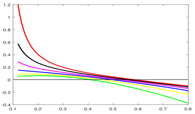
Figure 1: Plot of $h_{d}(D)$ against $D$ when $d=1$ with $\alpha=0.5$, $1$, …$3.0$.

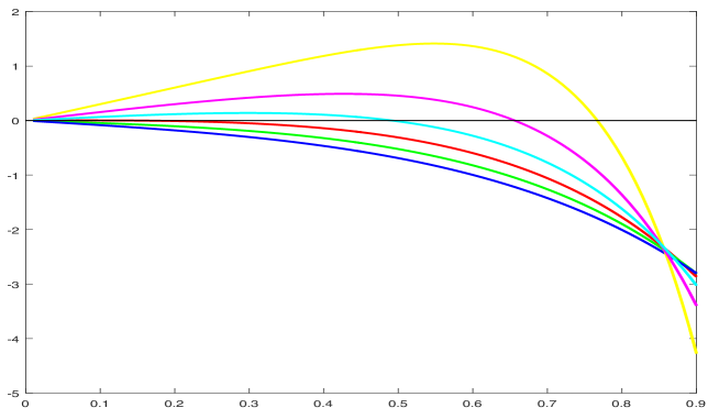
Figure 2: Plot of $u\mapsto\mathcal{H}(u)$ when $d=2$, $\alpha=2$, and $D=0.2$, $0.25$, …$0.45$. In this particular case, $D_{*}\approx 0.354$ solves $\left(8\,\operatorname{\Gamma}\left(\frac{3}{2},\frac{1}{8\,D}\right)-8\,\sqrt{\pi}\right)D-\operatorname{\Gamma}\left(\frac{1}{2},\frac{1}{8\,D}\right)+2\,\sqrt{\pi}=0$.

References

- [1] Barbaro, A. B. T., Cañizo, J. A., Carrillo, J. A., and Degond, P. Phase transitions in a kinetic flocking model of Cucker-Smale type. Multiscale Model. Simul. 14, 3 (2016), 1063–1088.
- [2] Barbaro, A. B. T., and Degond, P. Phase transition and diffusion among socially interacting self-propelled agents. Discrete Contin. Dyn. Syst. Ser. B 19, 5 (2014), 1249–1278.
- [3] Bolley, F., Cañizo, J. A., and Carrillo, J. A. Stochastic mean-field limit: non-Lipschitz forces and swarming. Math. Models Methods Appl. Sci. 21, 11 (2011), 2179–2210.
- [4] Bostan, M., and Carrillo, J. A. Asymptotic fixed-speed reduced dynamics for kinetic equations in swarming. Math. Models Methods Appl. Sci. 23, 13 (2013), 2353–2393.
- [5] Campos, J. F., and Dolbeault, J. Asymptotic estimates for the parabolic-elliptic Keller-Segel model in the plane. Comm. Partial Differential Equations 39, 5 (2014), 806–841.
- [6] Carrillo, J. A., McCann, R. J., and Villani, C. Kinetic equilibration rates for granular media and related equations: entropy dissipation and mass transportation estimates. Rev. Mat. Iberoamericana 19, 3 (2003), 971–1018.
- [7] Cucker, F., and Mordecki, E. Flocking in noisy environments. J. Math. Pures Appl. (9) 89, 3 (2008), 278–296.
- [8] Cucker, F., and Smale, S. Emergent behavior in flocks. IEEE Trans. Automat. Control 52, 5 (2007), 852–862.
- [9] Degond, P., Frouvelle, A., and Liu, J.-G. Macroscopic limits and phase transition in a system of self-propelled particles. J. Nonlinear Sci. 23, 3 (2013), 427–456.
- [10] Degond, P., Frouvelle, A., and Liu, J.-G. Phase transitions, hysteresis, and hyperbolicity for self-organized alignment dynamics. Arch. Ration. Mech. Anal. 216, 1 (2015), 63–115.
- [11] Frouvelle, A., and Liu, J.-G. Dynamics in a kinetic model of oriented particles with phase transition. SIAM J. Math. Anal. 44, 2 (2012), 791–826.
- [12] Tugaut, J. Phase transitions of McKean-Vlasov processes in double-wells landscape. Stochastics 86, 2 (2014), 257–284.
- [13] Vicsek, T., Czirók, A., Ben-Jacob, E., Cohen, I., and Shochet, O. Novel type of phase transition in a system of self-driven particles. Phys. Rev. Lett. 75 (Aug 1995), 1226–1229.