The Affective Factors on the Uncertainty in the Collisions of the Soliton Solutions of the Double Field sine-Gordon System

Abstract

Inspired by the well known sine-Gordon equation, we present a symmetric coupled system of two real scalar fields in $1+1$ dimensions. There are three different topological soliton solutions which be labelled according to their topological charges. These solitons can absorb some localized non-dispersive wave packets in collision processes. It will be shown numerically, during collisions between solitons, there will be an uncertainty which originates from the amount of the maximum amplitude and arbitrary initial phases of the trapped wave packets.

Keywords : sine-Gordon, coupling, nonlinear, soliton, wave packet, uncertainty.

I Introduction

Relativistic solitons, including those of the conventional sine-Gordon (SG) equation, exhibit remarkable similarities with classical particles. They exert short range forces on each other and make collisions, without losing their identities rajarama ; Das ; lamb ; Drazin . They are localized objects and do not disperse while propagating in the medium. The integrable SG system has been considered in recent investigations, it has various applications in many branches of physics Riazi1 ; a11 ; a12 ; a13 ; a14 ; a15 . Because of their wave nature, they do tunnel a barrier in certain cases, although this tunnelling is different from the well-known quantum version Riazi1 ; Riazi3 . Topological solitons are stable, due to the boundary conditions at spatial infinity. Their existence, therefore, is essentially dependent on the presence of degenerate vacua Lee .

Topology provides an elegant way of classifying solitons in various sectors according to the mappings between the degenerate vacua of the field and the points at spatial infinity. For the sine-Gordon system in $1+1$ dimensions, these mappings are between $\phi=n\pi$, $n\in Z$ and $x=\pm\infty$, which correspond to kinks and anti-kinks of the SG system.

Coupled systems of scalar fields have been investigated by many authors rajarama ; Bazeian ; Bazeia ; Riazi1 ; Riazi4 . Bazeia et al. Bazeia considered a system of two coupled real scalar fields with a particular self-interaction potential such that the static solutions are derivable from first order coupled differential equations. Riazi et al. Riazi4 employed the same method to investigate the stability of the single soliton solutions of a particular system of this type. Moreover, they used SG system to make a coupled system of two real scalar fields with a rich structure and dynamics Riazi1 .

Inspired by the well-known properties of the SG equation, we will introduce a symmetric coupled systems of two real scalar fields. It can be considered as two similar SG equations which are coupled to each other. It has three types of soliton solutions which are named $H$ (horizontal), $V$ (vertical) and $D$ (diagonal) solitons. $H$ and $V$ solutions are nothing but the usual SG kink (anti-kink) solutions. They can combine to other and form a $D$-soliton. Moreover, it will be shown numerically and analytically that a $H$ ($V$)-soliton can absorb small wave packets which evolve according to a Schrödinger like equation. These small wave packets do not make any considerable change in the particle aspects of a soliton but they have a main role in the collisions. These packets lead to an uncertainty in the collision processes related to trivial initial phases. In fact, initial phases behave like hidden variables which lead to different fates in the collision processes. Moreover, these wave-packets do not disperse and they satisfy a similar deBroglie’s wavelength-momentum relation Riazi .

Note that the term “soliton” is used throughout this paper for localized solutions. The problem of integrability of the model is not addressed here. Such non-dispersive solutions are called “lumps” by Coleman Coleman to avoid confusion with true solitons of integrable models. However, it has now become popular to use the term soliton in its general sense.

The organization of this paper is as follows: In section II, we introduce the lagrangian density, dynamical equations, and conserved currents of the proposed model. In section III, some exact and numerical solutions, together with the corresponding topological charges and energies are derived. The necessary nomenclature and the other properties of the single soliton solutions are also introduced in this section. In section IV, we proceed analytically to understand why a soliton can absorb a wave packet, and will provide a detailed discussion about the internal modes of each single soliton solution. In section V, we will see numerically an uncertainty in collision processes which originates from the wave aspect of the soliton solutions.

II DYNAMICAL EQUATIONS, CONSERVED CURRENTS, AND TOPOLOGICAL CHARGES

Within a relativistic formulation, the well known sine-Gordon (SG) equation for a real field ($\phi$) in 1+1 space-time dimensions can be written as

$$\Box\phi=-\sin(2\phi).$$ (1)

The factor $2$ in the argument of $\sin(2\phi)$ dose not change the main properties of the solutions and we have included it for convergence. This equation can be extracted from the following Lagrangian density:

$${\cal L}=\frac{1}{2}\partial_{\mu}\phi\partial^{\mu}\phi-\sin^{2}(\phi).$$ (2)

The special traveling wave solutions of this equation are topological objects which are called kinks and antikinks:

$$\phi_{v}(x,t)=\varphi(\gamma(x-vt))=2\tan^{-1}[\exp(\pm\sqrt{2}\gamma(x-vt))],$$ (3)

where $v$ is the velocity, $\gamma=1/\sqrt{1-v^{2}}$ and $+$ ($-$) is denoted for kinks (antikinks). For any kink (antikink) solution (3), the related localized energy density function is

$$\varepsilon(x,t)=2\hskip 2.13394pt{\rm sech}^{2}[\sqrt{2}\gamma(x-vt)].$$ (4)

Such solutions (3) are very stable and without any deformation reappear after collisions. In this respect, they can be imagined as non-interacting real particles in 1+1 space-time.

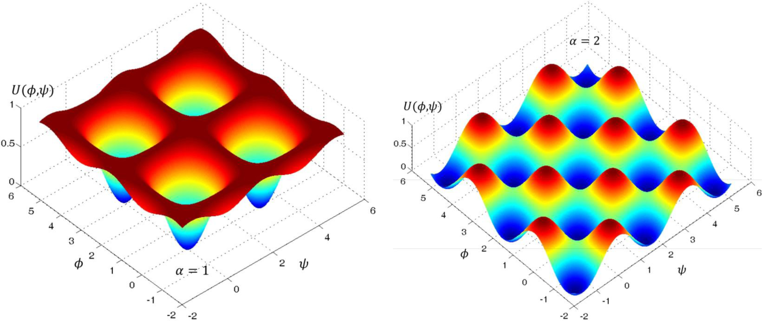
Figure 1: The 3D shape of the potential (6) for two special cases $\alpha=1$ and $\alpha=2$. It obvious that for the case $\alpha=1$, as a representative of the systems $\alpha<2$, the vacua are $(\phi,\psi)=(N_{1}\pi,N_{2}\pi)$, where $N_{1}$ and $N_{2}$ are any arbitrary integer number.

We employ the SG system to construct a new system in 1+1 space-time dimensions with two real scalar fields $\phi$ and $\psi$, by introducing a new Lagrangian density:

$${\cal L}=\frac{1}{2}\partial_{\mu}\phi\partial^{\mu}\phi+\frac{1}{2}\partial_{\mu}\psi\partial^{\mu}\psi-U(\phi,\psi),$$ (5)

where

$$U(\phi,\psi)=\sin^{2}(\phi)+\sin^{2}(\psi)-\alpha\sin^{2}(\phi)\sin^{2}(\psi),$$ (6)

is the field potential and $\alpha$ is a real constant parameter. The field potentials for two values of $\alpha=1$ and $\alpha=2$ are shown in Fig. 1. It is obvious that $\alpha$ controls the strength of interactions between fields $\phi$ and $\psi$. For example, if $\alpha=0$, there is no interaction between fields and we have two independent sine-Gordon (SG) field equations for $\phi$ and $\psi$. For low energy excitations ($\phi,\psi\ll 1$), the potential for the coupled fields can be expanded up to the fourth order:

$$U(\phi,\psi)\approx\phi^{2}+\psi^{2}-\alpha\phi^{2}\psi^{2}.$$ (7)

According to the standard quantum field theory, this leads to two equal mass terms $\phi^{2}$ and $\psi^{2}$, and a four legs interaction term $\alpha\phi^{2}\psi^{2}$.

From the Lagrangian density (5), we obtain the following equations for $\phi$ and $\psi$, respectively

$$\Box\phi=-\sin(2\phi)(1-\alpha\sin^{2}(\psi)),$$ (8)

and

$$\Box\psi=-\sin(2\psi)(1-\alpha\sin^{2}(\phi)).$$ (9)

Since the Lagrangian density (5) is Lorentz invariant, the corresponding energy-momentum tensor rajarama is

$$T_{\mu\nu}=\partial_{\mu}\phi\partial_{\nu}\phi+\partial_{\mu}\psi\partial_{\nu}\psi-\eta_{\mu\nu}{\cal L},$$ (10)

which satisfies the conservation law:

$$\partial_{\mu}T^{\mu\nu}=0.$$ (11)

In equation (10), $\eta_{\mu\nu}=\textrm{diag}(1,-1)$ is the metric of the 1 + 1 dimensional Minkowski space-time. The Hamiltonian (energy) density is obtained from Eq. (10) according to

$${\cal H}=\varepsilon(x,t)=T^{00}=\frac{1}{2}\dot{\phi}\dot{\phi}+\frac{1}{2}\phi^{{}^{\prime}}\phi^{{}^{\prime}}+\frac{1}{2}\dot{\psi}\dot{\psi}+\frac{1}{2}\psi^{{}^{\prime}}\psi^{{}^{\prime}}+U(\phi,\psi),$$ (12)

in which dot and prime denote differentiation with respect to $t$ and $x$, respectively. Note that we have assumed c=1 throughout this paper. Moreover, the following topological currents can be defined:

$$J_{V}^{\mu}=C_{1}\epsilon^{\mu\nu}\partial_{\nu}\phi,\quad J_{H}^{\mu}=C_{2}\epsilon^{\mu\nu}\partial_{\nu}\psi,$$ (13)

where $\epsilon^{\mu\nu}$ is the completely antisymmetric tensor and $C_{1}$ and $C_{2}$ are arbitrary constants. The subscripts $H$, $V$ and $D$, denote “horizontal”, “vertical” and “diagonal” which will be explained later. These currents ($J_{H,V}^{\mu}$) are conserved independently:

$$\partial_{\mu}J_{V}^{\mu}=0,\quad\partial_{\mu}J_{H}^{\mu}=0,$$ (14)

and lead to quantized constant topological charges. The corresponding topological charges are given by:

$$Q_{V}=\int_{-\infty}^{+\infty}J_{V}^{0}dx=C_{1}[\phi(+\infty)-\phi(-\infty)],$$ (15)

$$Q_{H}=\int_{-\infty}^{+\infty}J_{H}^{0}dx=C_{2}[\psi(+\infty)-\psi(-\infty)].$$ (16)

In this paper, we set $C_{1}=C_{2}=\frac{1}{\pi}$, for convenience.

III SINGLE-SOLITON SOLUTIONS

Each static stable soliton solution should vary between two neighbouring vacuum points and its energy must be minimum among infinite ways which can connect the two vacua, i.e. they must be stationary. Namely, if we consider the systems which were introduced in the previous section, it is easy to show that there are three kinds of static soliton solutions: $H$ (horizontal), $V$ (vertical) and $D$ (diagonal) types, depending on the beginning and ending points of the solution on the $(\phi,\psi)$ plane Riazi1 . They are shown symbolically in Fig. 2.

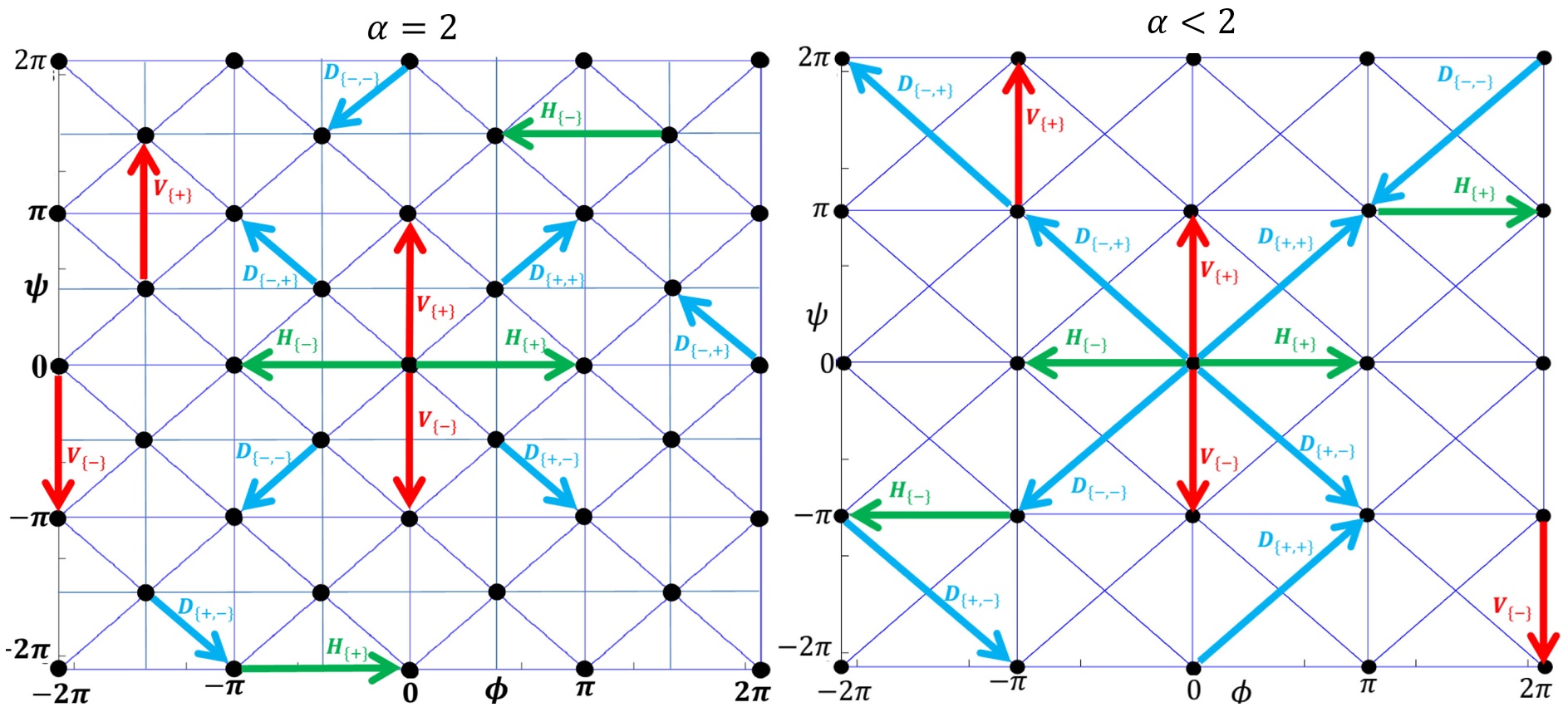
Figure 2: According to Fig. 1, if one considers just the vacuum points, a mesh of the regular points is obtained on the $(\phi,\psi)$ plane. Black points are correspond to vacua. Nomenclature of horizontal (H), vertical (V) and diagonal (D) solutions according to the boundary conditions on the $(\phi,\psi)$ plane. Each line which connects two neighbouring vacua can be correspond to a stationery soliton solution. It is easy to understand there are infinite soliton solutions. Note that the subscripts $\{+\}$ ($\{-\}$) is used for a kink (antitank) solution.

In general, there are two scalar fields $\phi$ and $\psi$ which are coupled together via the dynamical equations (8) and (9). For three special situations, these coupled equations reduce to simple formats. First, if one sets $\psi=N_{2}\pi$ ($N_{2}=0,\pm 1,\pm 2,\cdots$), Eq. (9) is satisfied automatically and Eq. (8) turns to the same original SG equation (1) with the same well-known kink ($H_{\{+\}}$) and antikink ($H_{\{-\}}$) solutions (3). Second, on the contrary, for a fixed value of $\phi=N_{1}\pi$ ($N_{1}=0,\pm 1,\pm 2,\cdots$), Eq. (8) is satisfied automatically and Eq. (9) leads to the same kink ($V_{\{+\}}$) and antikink ($V_{\{-\}}$) solutions (3) as well. Third, if one considers the situations for which $\phi=\pm\psi+N_{1}\pi$ or $\psi=\pm\phi+N_{2}\pi$ (i.e. $D$-solitons), Eqs. (8) and (9) both turn to an identical dynamical equation as follows:

$$\Box\phi=-\sin(2\phi)(1-\alpha\sin^{2}(\phi))=-\dfrac{d{\cal U}}{d\phi},$$ (17)

where

$${\cal U}(\phi)=\sin^{2}(\phi)-\frac{\alpha}{2}\sin^{4}(\phi),$$ (18)

is considered as a new field potential just for $D$-solitons. This potential (18) for $\alpha\leq 2$ is always positive and its vacua are $\phi=N\pi$ ($N=0,\pm 1,\pm 2,\cdots$). It again, depending on $\alpha$, leads to new types of the kink and antikink solutions which unfortunately we could not find their explicit forms at all. However, by a Runge-Kutta method, one can simply obtain them numerically (see Figs. 3 and 4). Thus, the evolution of such solutions ($D$-solitons) can be simulated by a single non-linear field equation (17). Fortunately for case $\alpha=2$, the PDE (17) reduces to a new version of the SG equation:

$$\Box\phi=-\frac{1}{2}\sin(4\phi)=-\dfrac{d}{d\phi}[\frac{1}{4}\sin^{2}(2\phi)],$$ (19)

for which ${\cal U}(\phi)=\frac{1}{4}\sin^{2}(2\phi)$. The $D$-soliton solutions of this equation (19) are presented in Table. 2. The rest energy in this case can be calculated easily equal to $E_{o}=\sqrt{2}$ which is exactly half of $H$ and $V$ rest energy.

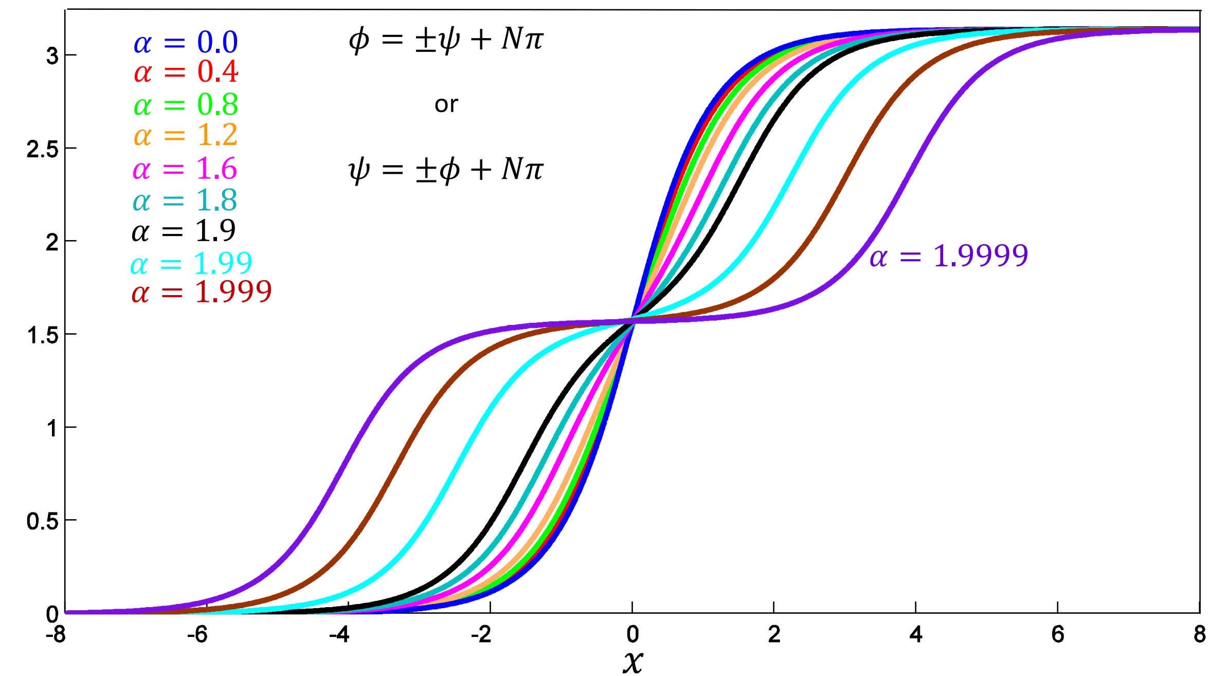
Figure 3: For different $\alpha$’s, there are different $D$-soliton solutions.

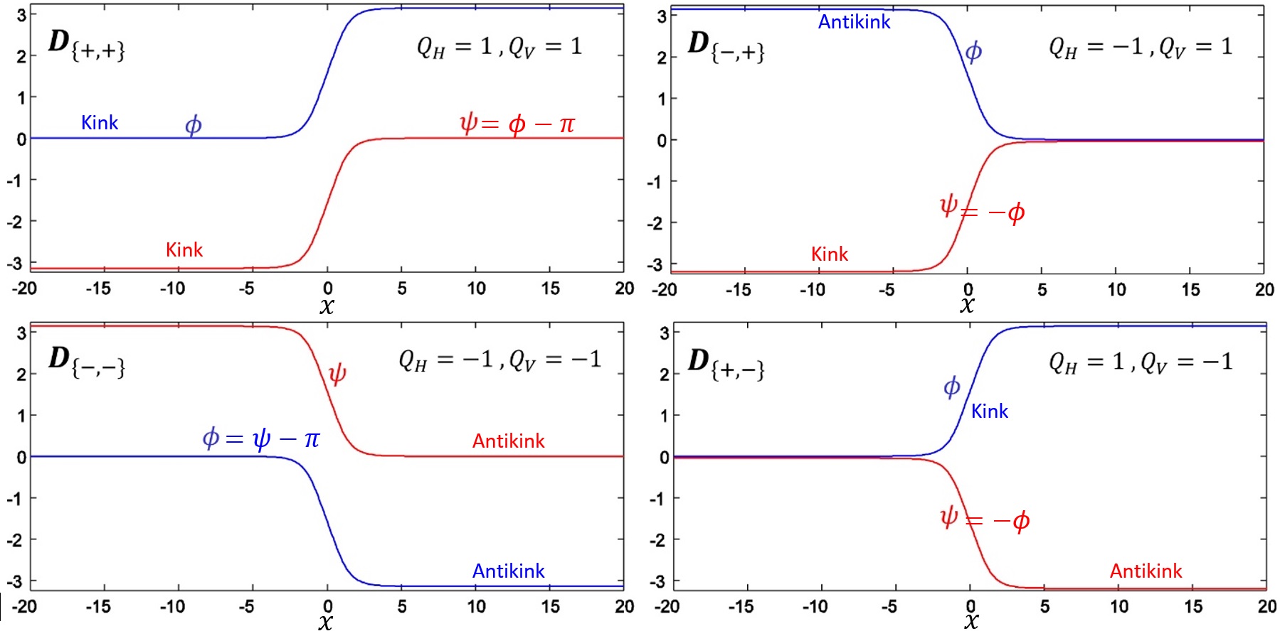
Figure 4: There are four types of D-soliton solutions for $\alpha=1$ (as a representative of the systems with $\alpha<2$) which are characterized by different permutations of $Q_{H}$ and $Q_{V}$ signs. In other words, they are characterized to four different combinations of the kinks and antikinks related to fields $\phi$ and $\psi$.

Briefly, there are two different types of $H$ ($V$)-solitons which are denoted by $H_{\{+\}}$ ($V_{\{+\}}$) and $H_{\{-\}}$ ($V_{\{-\}}$). The subscript $\{+\}$ ($\{-\}$) is refereed to a kink (anti-kink) with positive (negative) topological charge. All exact static $H$ and $V$-solitons and their features are summarized in Table. 1. If a kink or anti-kink of $\phi$ field lives with another kink or anti-kink of $\psi$ field, we have a $D$-soliton. There are 4 types of $D$-solitons which correspond to different combinations of kink or anti-kink for $\phi$ and $\psi$. Namely, a $D_{\{+,-\}}$-soliton is composed of a kink with $Q_{H}>0$ for the $\phi$ field beside an anti-kink with $Q_{V}<0$ for the $\psi$ field. In an equivalent statement, the first and second subscript in a $D$-soliton is used to characterize $Q_{H}$ and $Q_{V}$ signs respectively (see Fig. 4).

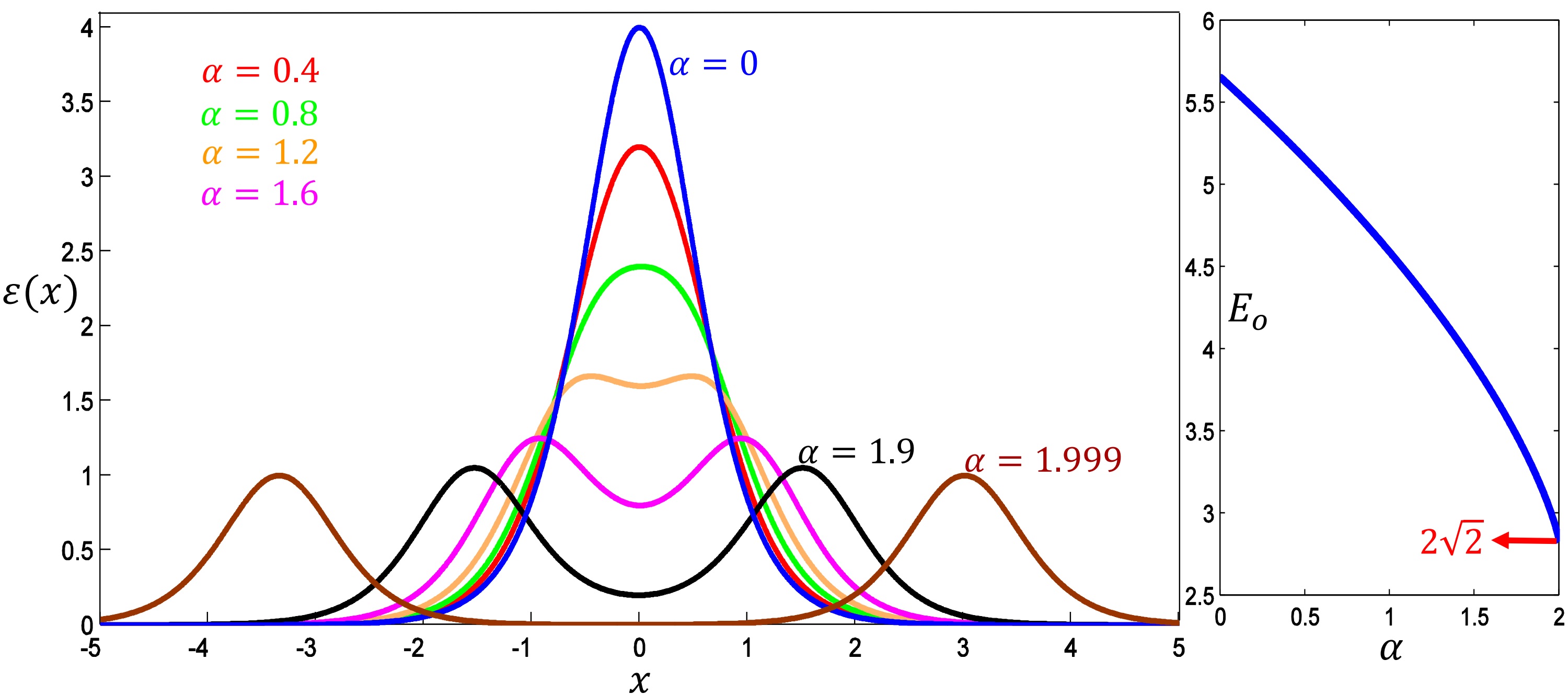
Figure 5: The curves in the left hand side are the energy density functions for different non-moving D-solitons. The right hand side is the rest energy of the $D$-solitons versus $\alpha$.

Type	Solution	$Q_{H}$	$Q_{V}$	$E_{o}$
$H_{\{\pm\}}$	$\phi=2\tan^{-1}[\exp(\pm\sqrt{2}x)]+N_{1}\pi,\quad\quad\psi=N_{2}\pi$	$\pm 1$	$0$	$2\sqrt{2}$
$V_{\{\pm\}}$	$\phi=N_{1}\pi,\quad\quad\psi=2\tan^{-1}[\exp(\pm\sqrt{2}x)]+N_{2}\pi$	$0$	$\pm 1$	$2\sqrt{2}$

Table 1: Exact static soliton solutions of the systems $\alpha<2$ and the corresponding horizontal and vertical topological charges and rest energies. $N_{1}$ and $N_{2}$ are just arbitrary integer constants.

Type	Solution	$Q_{H}$	$Q_{V}$	$E_{0}$
$H_{\{\pm\}}$	$\phi=2\tan^{-1}[\exp(\pm\sqrt{2}x)]+\dfrac{N_{1}\pi}{2},\quad\psi=\dfrac{2N_{2}+N_{1}}{2}\pi$	$\pm 1$	$0$	$2\sqrt{2}$
$V_{\{\pm\}}$	$\phi=\dfrac{2N_{1}+N_{2}}{2}\pi,\quad\psi=2\tan^{-1}[\exp(\pm\sqrt{2}x)]+\dfrac{N_{2}\pi}{2}$	$0$	$\pm 1$	$2\sqrt{2}$
$D_{\{\pm,\pm\}}$	$\phi=\pm\psi+N_{2}\pi=\tan^{-1}[\exp(\pm\sqrt{2}x)]+\dfrac{N_{1}\pi}{2}$	$\pm\frac{1}{2}$	$\pm\frac{1}{2}$	$\sqrt{2}$

Table 2: Exact static soliton solutions and the corresponding horizontal and vertical topological charges and rest energies for case $\alpha=2$ . $N_{1}$ and $N_{2}$ are just arbitrary integer constants.

The rest energy of a soliton solutions is obtained by integration of the static kink energy density

$$E_{o}=\int_{-\infty}^{+\infty}\varepsilon(x)dx.$$ (20)

The rest energy of $H$ and $V$-soliton solutions for systems with $\alpha\leq 2$ all are equal to $E_{o}=2\sqrt{2}$. But for different $D$-solitons which are identified with different $\alpha$’s (Fig. 3), there are different energy density functions and rest energies (see Fig. 5).

From now, we only consider systems with a genuine interaction between their components ($\phi$ and $\psi$ fields), i.e. those for which $\alpha<2$ (except $\alpha=0$). All systems which are within this range have identical vacua and the right part of Fig. 2 ($\alpha=1$) can be generalized for all of them.

IV INTERNAL MODES

In this section, analytically and numerically, we showed that $H$, $V$ and $D$-solitons can keep a constantly oscillating behaviour for $0<\alpha<2$. In similar situations DC ; G ; Riazi4 ; OV ; GH ; MM1 , these oscillations have been interpreted as low energy trapped wave packets (see Fig. 6). Numerically, it was seen that for systems with $\alpha<0$, there are no long lasting oscillations.

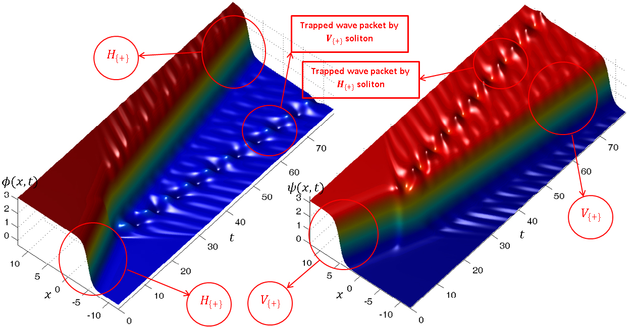
Figure 6: A $V$ ($H$)-soliton can trap a wave packet from the $\phi$ ($\psi$) field for systems with $0<\alpha<2$. This special Fig is the field representation of a $H_{\{+\}}-V_{\{+\}}$ collision for $\alpha=1.2$ with initial speed $v=0.3$. Note that, the shape of the kinks themselves stay almost unchanged.

To provide a quantitative discussion of this phenomenon we follow the standard procedure and apply a small oscillatory perturbation to a non-moving $H$-soliton solution Bazeia ; Riazi4 :

$$\phi_{o}(x,t)=\varphi(x)+\Phi(x)e^{-i(\Omega_{o}t-\beta)}+N_{1}\pi,\quad\quad\psi_{o}(x,t)=N_{2}\pi+\Psi(x)e^{-i(\omega_{o}t-\theta)}.$$ (21)

in which $\varphi(x)=2\tan^{-1}[\exp(\pm\sqrt{2}x)]$ is the same exact non-moving soliton solution (3), $\Phi$ (x) and $\Psi(x)$ are small perturbations, $\theta$ and $\beta$ are arbitrary constant phases. Similarly, a little disturbed non-moving $V$-soliton can be shown as follows:

$$\phi_{o}(x,t)=N_{1}\pi+\Phi(x)e^{-i(\Omega_{o}t-\beta)},\quad\quad\psi_{o}(x,t)=\varphi(x)+\Psi(x)e^{-i(\omega_{o}t-\theta)}+N_{2}\pi.$$ (22)

However, inserting the little disturbed non-moving $H$-soliton (21), as an ansatz, into the non-linear differential equations (8) and (9) and expanding to the first order in $\Psi$ and $\Phi$, we obtain two independent eigenvalue equations for $\Psi$ and $\Phi$ respectively, which look like the Schrödinger equation:

$$-\frac{d^{2}\Psi}{dx^{2}}+V_{1}(x)\Psi=\omega_{o}^{2}\Psi,$$ (23)

and

$$-\frac{d^{2}\Phi}{dx^{2}}+V_{2}(x)\Phi=\Omega_{o}^{2}\Phi,$$ (24)

where

$$V_{1}(x)=2-2\alpha\sin^{2}(\varphi)=2-2\alpha\hskip 2.13394pt{\rm sech}^{2}(\sqrt{2}x).$$ (25)

and

$$V_{2}(x)=\dfrac{d^{2}[\sin^{2}(\varphi)]}{d\varphi^{2}}=2-4\hskip 2.13394pt{\rm sech}^{2}(\sqrt{2}x).$$ (26)

It is easy to show that for the Schrödinger-like equation (24) with the well-known potential (26), there is just a trivial solution $\Phi(x)=\xi\dfrac{d\varphi}{dx}$ which corresponds to $\Omega_{o}=0$, and $\xi$ is just any arbitrary small number to be sure that $|\Phi|\ll 1$. In fact, this potential (26) is related to the well-known SG system which were studied completely in Refs. GH ; MM1 . According to Eq. (21), it is easy to show that this trivial solution (i.e. $\Phi(x)=\xi\dfrac{d\varphi}{dx}$ and $\Omega_{o}=0$) dose not have physical meaning and is just associated with an infinitesimal translation of the static $H$-soliton:

$$\phi_{o}(x)=\varphi(x)+\xi\frac{d\varphi_{o}}{dx}=\varphi(x+\xi).$$ (27)

In other words, for the Schrödinger-like Eq. (24) there is not any non-trivial solution corresponds to a channel to impose some permanent oscillations, hence for a single $H$ ($V$)-soliton, $\Phi$ ($\Psi$) must be always equal to zero and the shape of the kinks and antikinks themselves remain unchanged (see Fig. 6).

Instead, the Schrödinger-like equation (23) with the potential (25) can be solved numerically, using a Runge-kutta method. It was shown that numerically for any arbitrary $\alpha$ ($0<\alpha<2$), the Schrödinger-like equation (23) leads to a single bound state (internal mode) as a non-trivial localized solution with a special eigenvalue $0<\omega_{o}^{2}<2$ (see Fig. 7).

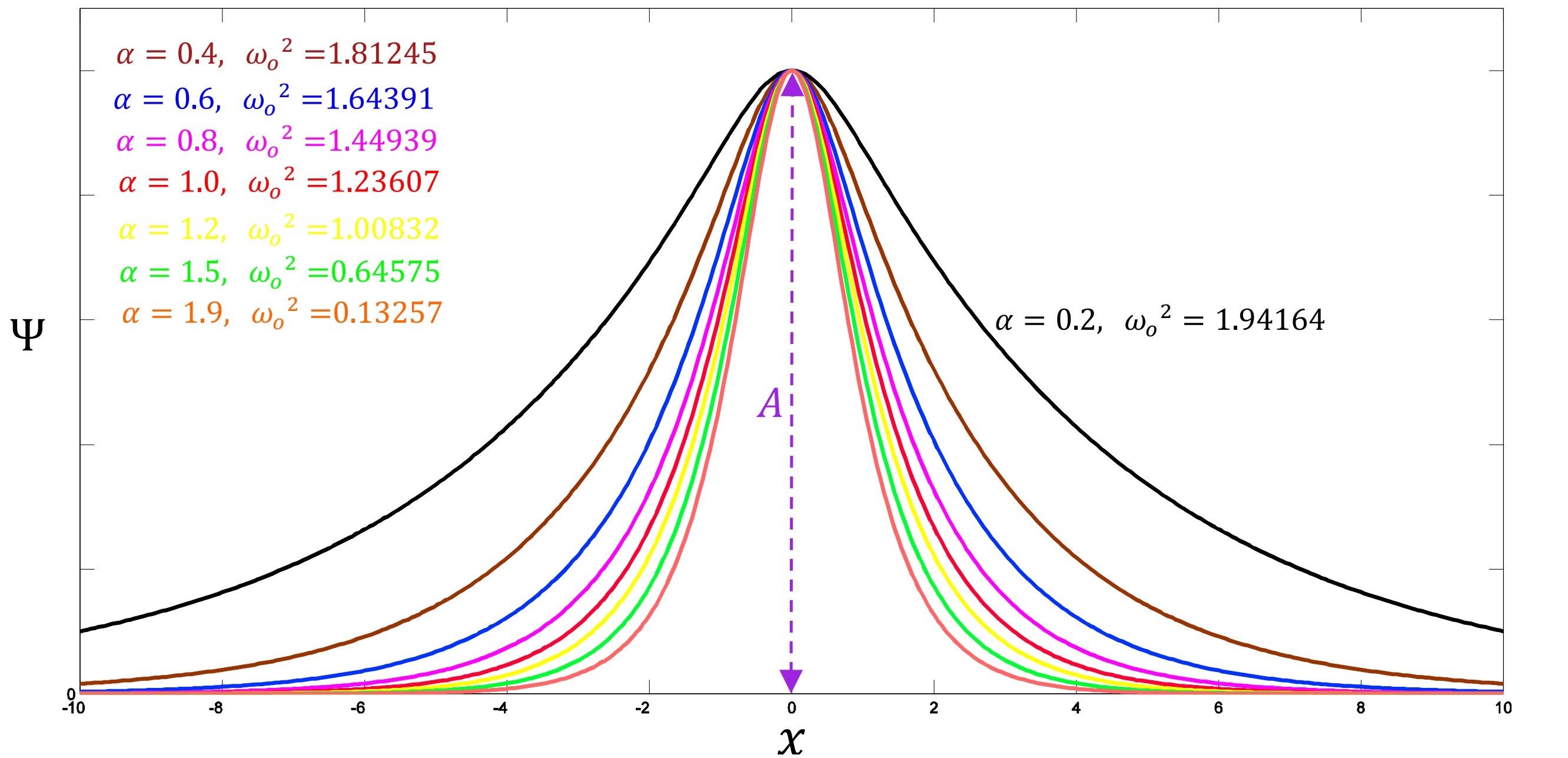
Figure 7: For any arbitrary $\alpha$ ($0<\alpha<2$), the eigenvalue equation (23) leads to a single bound state (eigenfunction) $\Psi$ with a special eigenvalue $0<\omega_{o}^{2}<2$. Here, $A=\max(|\Psi|)$ is the maximum amplitude of the eigenfunction $\Psi$ (trapped wave packet). The existence of this bound state is the reason why we can see a permanent oscillation after collisions in Fig. 6 for $H$-soliton. A similar reason exists for justifying the imposed oscillation on the $V$-soliton in Fig. 6.

Therefore, for a $H$ ($V$)-soliton there is a single non-trivial bound state $\Psi$ ($\Phi$) with $0<\omega_{o}^{2}<2$ ($0<\Omega_{o}^{2}<2$), but $\Phi=0$ ($\Psi=0$). In other words, a $H$ ($V$)-soliton provides an attractive potential $V_{1}(x)$ which can trap some small localized waves of the adjacent field $\psi$ ($\phi$). The other cases for which $\alpha<0$, we are faced with a potential barrier which cannot have any bound state. Accordingly, one can understand easily why for $H$ ($V$)-solitons with $0<\alpha<2$, there is a permanent oscillation after collisions, because for such solutions there is an internal mode which can be considered as a channel for trapping external energies and imposing some permanent oscillations. Note that contrary to many double-field nonlinear systems, the two linear equations (23) and (24) are decoupled to first order in fields and linear perturbations of each field do not see companion field to first order.

Note that the rest energy of a little disturbed $H$ ($V$)-soliton, with a good approximation, is equal to the same undisturbed ones. In general, a little disturbed non-moving $H$-soliton can be expressed as follows:

$$\phi_{o}(x,t)=\varphi(x)+\delta\phi(x,t)+N_{1}\pi,\quad\quad\psi_{o}(x,t)=N_{2}\pi+\delta\psi(x,t),$$ (28)

where $\delta\phi(x,t)$ and $\delta\psi(x,t)$ can be considered any arbitrary permissible small deformations (variations). Note that, the ansatz (21) is a special kind of the general form (28). If one inserts theses deformed functions (28) into the energy density function (12) and keeps the terms with the first order of variations, it yields:

$$\delta\varepsilon(x,t)=\varphi^{{}^{\prime}}(\delta\phi)^{{}^{\prime}}+(\delta\phi)\frac{dU(\varphi,N_{2}\pi)}{d\varphi}.$$ (29)

Note that, for a non-moving $H$ ($V$)-soliton, it is obvious that $\dot{\varphi}=0$ and $\frac{\partial U}{\partial\psi}$ ($\frac{\partial U}{\partial\phi}$) for $\psi=N_{2}\pi$ ($\phi=N_{1}\pi$) would be zero. Moreover, from Eq. (8) for a non-moving $H$-soliton, it is easy to show that $\varphi^{{}^{\prime\prime}}=\frac{dU(\varphi,N_{2}\pi)}{d\varphi}$. Therefore, Eq. (29) is simplified to

$$\delta\varepsilon(x,t)=\varphi^{{}^{\prime}}\delta\phi^{{}^{\prime}}+(\delta\phi)\varphi^{{}^{\prime\prime}}=\frac{d}{dx}(\varphi^{{}^{\prime}}\delta\phi)=\frac{d}{dx}(F).$$ (30)

where $F=\varphi^{{}^{\prime}}\delta\phi$. Since $\varphi^{{}^{\prime}}$ is zero at $x=\pm\infty$, then the change in the rest energy, to the first order of variations, would be

$$\delta E_{o}=\int_{-\infty}^{\infty}\delta\varepsilon(x,t)dx=F(\infty)-F(-\infty)=0.$$ (31)

Thus, to the first order of variations $\delta E_{o}$ would be zero. If one considered the second order of variations, $\delta E_{o}$ is not zero anymore, but it is very small. Hence, the increase of the total rest energy for a small deformed $H$ ($V$)-soliton (28) is approximately equal to zero, i.e. the rest energy of a little disturbed $H$ ($V$)-soliton is approximately equal to the undisturbed one.

We know that $\phi$ and $\psi$ are both scalars, then a moving perturbed $H$-soliton should be written generally in the following form:

$$\phi_{v}(x,t)=\varphi(\gamma(x-vt))+N_{1}\pi,\quad\quad\psi_{v}(x,t)=N_{2}\pi+\Psi(\gamma(x-vt))e^{i(kx-\omega t+\theta)},$$ (32)

where $kx-\omega t=k_{\mu}k^{\mu}$ is a scalar. If they are inserted into equation (9) and expanding it to the first order in $\Psi$, we obtain

$$(v^{2}\gamma^{2}\frac{d^{2}\Psi}{d\tilde{x}^{2}}+2iv\omega\gamma\frac{d\Psi}{d\tilde{x}}-\omega^{2}\Psi)e^{i(kx-\omega t+\theta)}-(\gamma^{2}\frac{d^{2}\Psi}{d\tilde{x}^{2}}+2ik\gamma\frac{d\Psi}{d\tilde{x}}-k^{2}\Psi)e^{i(kx-\omega t+\theta)}$$

$$=(-2+2\alpha\sin^{2}(\varphi))\Psi e^{i(kx-\omega t+\theta)},$$ (33)

where $\tilde{x}=\gamma(x-vt)$. Omitting the common exponential factor from both sides and equating the real and imaginary parts of the equation to zero separately, we obtain

$$k=\omega v,$$ (34)

and

$$-\frac{d^{2}\Psi}{d\tilde{x}^{2}}+V(\tilde{x})\Psi=(\omega^{2}-k^{2})\Psi=\omega_{o}^{2}\Psi.$$ (35)

One can simply use Eq. (34) and the fact that $kx-\omega t=k_{\mu}x^{\mu}$ is a scalar to obtain

$$\omega=\gamma\omega_{o}.$$ (36)

Moreover, it is easy to show that there is a similar relationship for relativistic energy of soliton solutions, i.e. $E=\gamma E_{o}$. Therefore, frequency and energy have the same behavior and we can relate them via introducing a Planck-like constant $\overline{h}$:

$$E=\overline{h}\omega.$$ (37)

Similarity, it is possible to find a relation between relativistic momentum of a soliton solution and wave number $k$:

$$p=\int_{-\infty}^{+\infty}T^{01}dx=mv=\overline{h}k.$$ (38)

This equation is very interesting, since it resembles the deBroglie’s relation.

$D$-solitons can also take an oscillating form after collisions. For a $D$-soliton the related dynamical equation and potential term were presented in Eqs. (17) and (18) respectively. In a similar way, we add a small time dependent oscillatory term to the static solution as a new one:

$$\phi_{o}(x,t)=\chi(x)+\Phi(x)e^{-i(\omega_{o}t-\theta)},$$ (39)

in which $\chi$ is the static kink (anti-kink) solution of Eq. (17), i.e. the ones which are shown in the Fig. (3). We can now substitute this ansatz (39) in the wave equation (17) and expand the potential by keeping only the linear terms in $\Phi$. Finally, the same Schrödinger-like eigenvalue equation is obtained again

$$-\frac{d^{2}\Phi}{dx^{2}}+V(x)\Phi=\omega_{o}^{2}\Phi,$$ (40)

where

$$V(x)=\dfrac{d^{2}{\cal U}(\chi)}{dx^{2}}$$ (41)

and ${\cal U}(\chi)=\sin^{2}(\chi)-\frac{\alpha}{2}\sin^{4}(\chi)$. For such systems, again there is a trivial solution $\Phi=\xi\dfrac{d\chi}{dx}$ with $\omega_{o}=0$ DC ; G ; Riazi4 ; OV ; GH ; MM1 . Moreover, it can be shown numerically that for systems with $0<\alpha<2$, there is a non-trivial internal mode which can be interpret as a physical channel for absorbing fluctuations and generates permanent oscillations in $D$-solitons. Finally, for a moving perturbed $D$-soliton, the corresponding results are exactly the same as those obtained for a perturbed $H$ and $V$-solitons.

The fore-mentioned results reveal further the interesting wave-particle aspects of solitons. Moreover, we will show numerically in the next section how the wave aspect can cause an uncertainty in the outcome of collisions.

V UNCERTAINTY IN COLLISIONS

If a small wave packet can be absorbed by a soliton, we will have an disturbed soliton. To study a disturbed $H-V$ collision with initial speed $v$, for which at least one of the $H$ and $V$-solitons get excited, we first need to prepare proper initial conditions for $\phi$ and $\psi$ fields in the following form

$$\phi_{v}(x,t)=\varphi(\gamma[(x-a)-vt])+\Phi(\gamma[(x-b)+vt])\cos{(kx-\Omega t+\theta_{1})},$$

$$\psi_{v}(x,t)=\varphi(\gamma[(x-b)+vt])+\Psi(\gamma[(x-a)-vt])\cos{(-kx-\omega t+\theta_{2})},$$ (42)

where $a$ and $b$ are initial positions provided $b-a$ is large enough and $\theta_{1}$ and $\theta_{2}$ can be some arbitrary initial phases. The small eigenfunctions $\Phi$ and $\Psi$, and eigenfrequency $\Omega=\omega=\gamma\omega_{o}=\gamma\Omega_{o}$, can be obtained easily by a straightforward Runge-Kutta method for Eq. (23). One can see Fig. 8 at $t=0$ for better understanding.

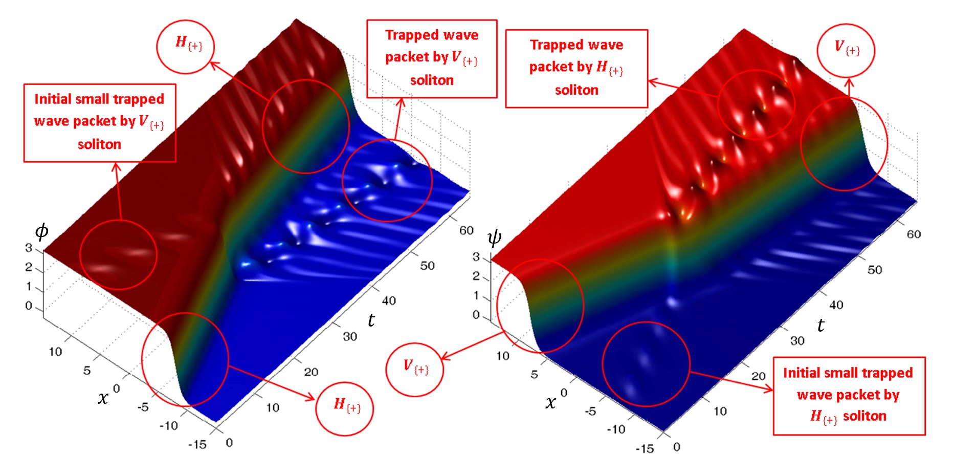
Figure 8: $\phi$ and $\psi$ representation of a disturbed $H_{\{+\}}-V_{\{+\}}$ collision with $0.3$ initial speed for which $\alpha=1.2$ and $b=-a=8$. The initial phases of the small trapped wave packets are $\theta_{1}=0$ and $\theta_{2}=0$. At $t=0$ the initial small trapped wave packet by $H_{\{+\}}$ ($V_{\{+\}}$) is the same oscillatory term $\Psi\cos{(-kx-\omega t+\theta_{2})}$ ($\Phi\cos{(kx-\Omega t+\theta_{1})}$) in Eq. (V).

The small wave packets does not seem to cause a considerable change in the particle aspect of a soliton. We consider wave packets which lead to less than $0.3$ percent change in the soliton energy. It was observed numerically that these small wave packets can have a considerable affect on the collision fate. For example, for an arbitrary system with $\alpha=1$, if one considers a disturbed pair $H_{\{+\}}$-$V_{\{-\}}$ which both initially trap small wave-packets with the same maximum amplitude ($A=\textrm{max}(|\Phi|)=\textrm{max}(|\Psi|)$) and initial phases $\theta_{1}=\theta_{2}=0$, when they are initialized to be at $a=-b=-11.9$ with $v=0.3$, depending on different values for the maximum amplitude $A$, there are different fates for the collision (see Fig. 9).

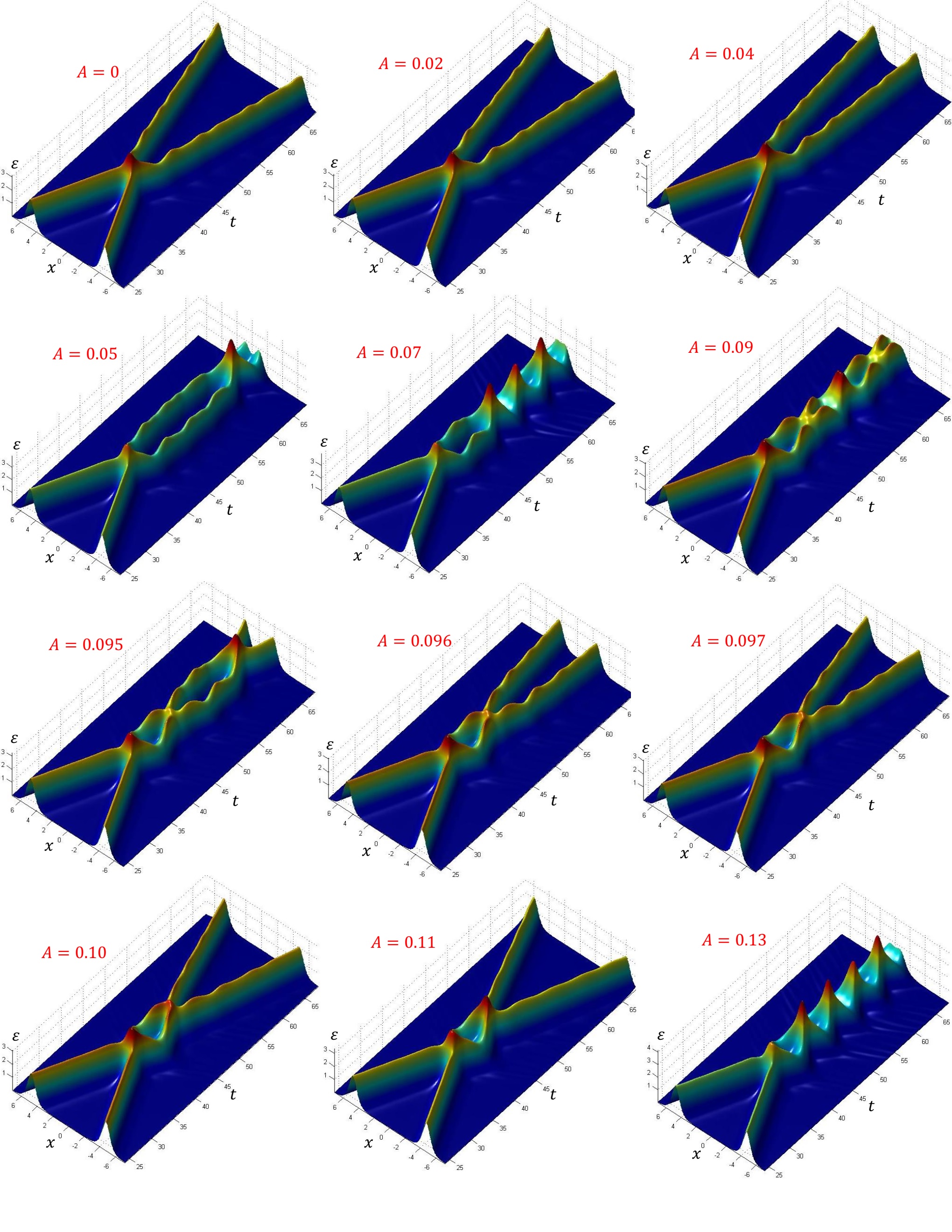
Figure 9: Energy density representations of a disturbed $H_{\{+\}}-V_{\{-\}}$ collision. We have set $v=0.3$, $\alpha=1$, $a=-11.9$, $b=11.9$ and $\theta_{1}=\theta_{2}=0$. They show that different maximum amplitude of the initial small trapped wave packets lead to different fates of the collision.

One might think that $\theta$ as an optional initial phase is an unimportant parameter. In fact, it has no role in determining basic physical features of a single soliton such as energy, momentum, topological charge and eigenvalues $\omega_{o}^{2}$. But, it was seen numerically during the collision between disturbed solitons, these initial phases become very important. For example, similar to Fig. 6 as an undisturbed $H_{\{+\}}$-$V_{\{+\}}$ collision, one can study a new disturbed version for which the amplitudes of the initial small trapped wave packets be equal to $A=0.04$. Hence, if one sets $a=-b=-8$, $\alpha=1.2$ and $v=0.3$, it was shown numerically that related to different initial phases, different fates will happen. Namely, for $\theta_{1}=\theta_{2}=0$, solitons are scattered from each other and reappear after collision, but with a periodic oscillations in the amplitude of their energy density functions (see Fig. 8 and the left hand side of Fig. 11). If $\theta_{1}=0$ and $\theta_{2}=\frac{\pi}{2}$, they capture each other and make a disturbed D-soliton (see Fig. 10 and the right hand side of Fig. 11).

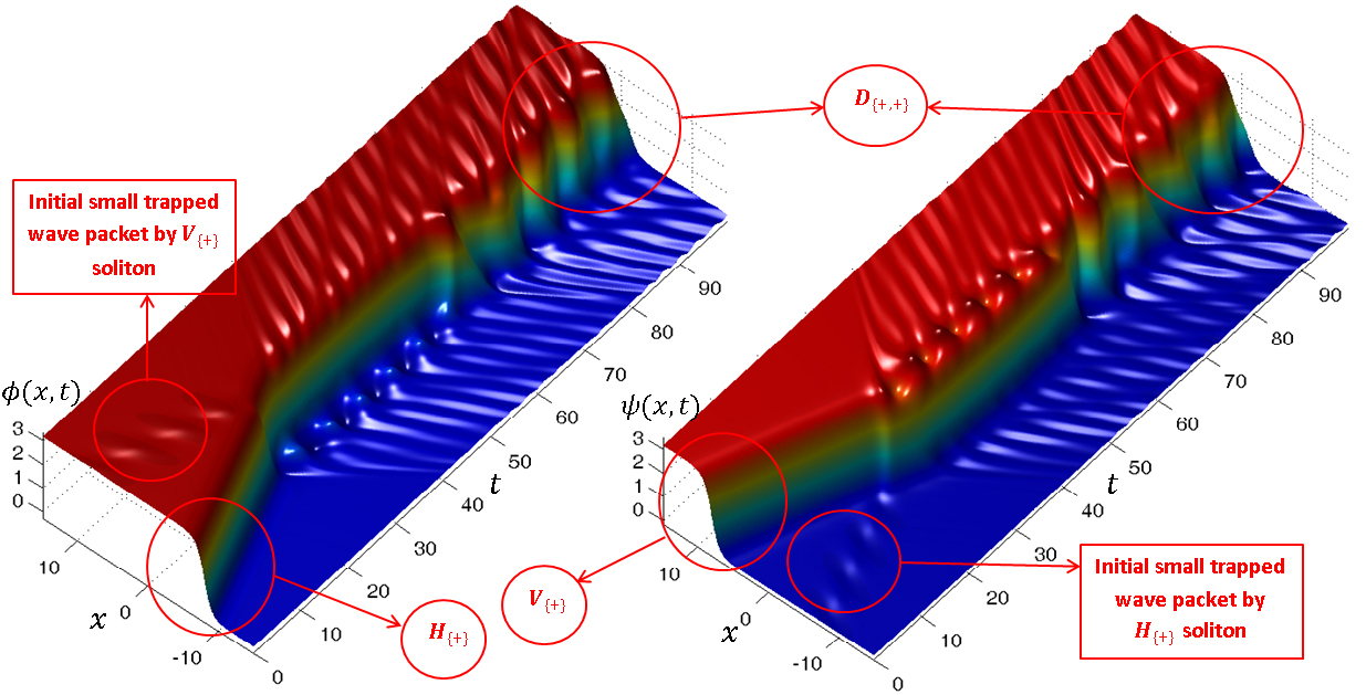
Figure 10: $\phi$ and $\psi$ representation of a disturbed $H_{\{+\}}-V_{\{+\}}$ collision with $0.3$ initial speed for which $\alpha=1.2$ and $a=-b=8$. The initial phases of the trapped wave packets are $\theta_{1}=0$ and $\theta_{2}=\frac{\pi}{2}$.

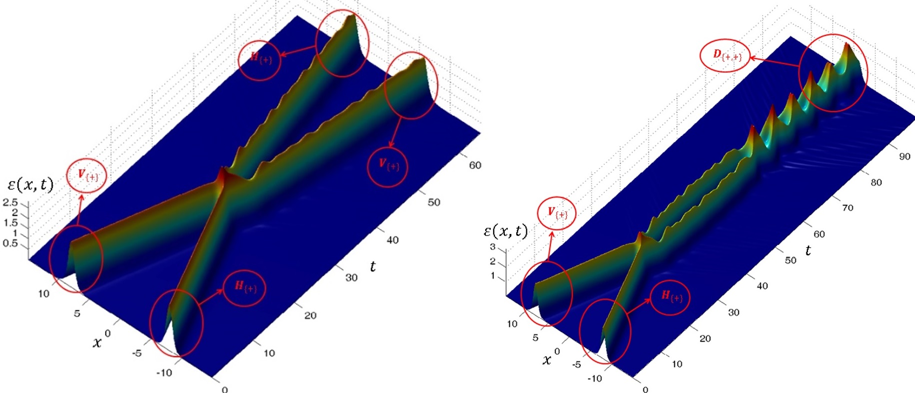
Figure 11: Energy density representation of a disturbed $H_{\{+\}}-V_{\{+\}}$ collision with $0.3$ initial speed for which $\alpha=1.2$ and $a=-b=8$. The initial phases for the trapped wave packets of the left (right) Fig are $\theta_{1}=0$ and $\theta_{2}=\frac{\pi}{2}$ ($\theta_{1}=0$ and $\theta_{2}=\frac{\pi}{2}$).

In a more complete example, to show numerically how such initial phases lead to different fates in a collision process, we can study many disturbed $H_{\{+\}}-V_{\{-\}}$ collisions with different arbitrary initial phases of a system with $\alpha=1.7$ for which $a=-24.5$, $b=24.5$, $A=0.05$ and $v=0.2$. Now, without any change in the physical features of the initial functions (V), we are free to choose any value for the initial phases $\theta_{1}$ and $\theta_{2}$. The different results of the collision for different initial phases can be seen in Fig. 12. Again, it demonstrates that different initial phases lead to different fates of the collision. Then, both capture and scattering can occur depending on the initial phases $\theta_{1}$ and $\theta_{2}$. It is reasonable to expect that if the amplitude of the initial tapped wave packets tend to zero the influence of initial phases on the collisions tends to zero as well.

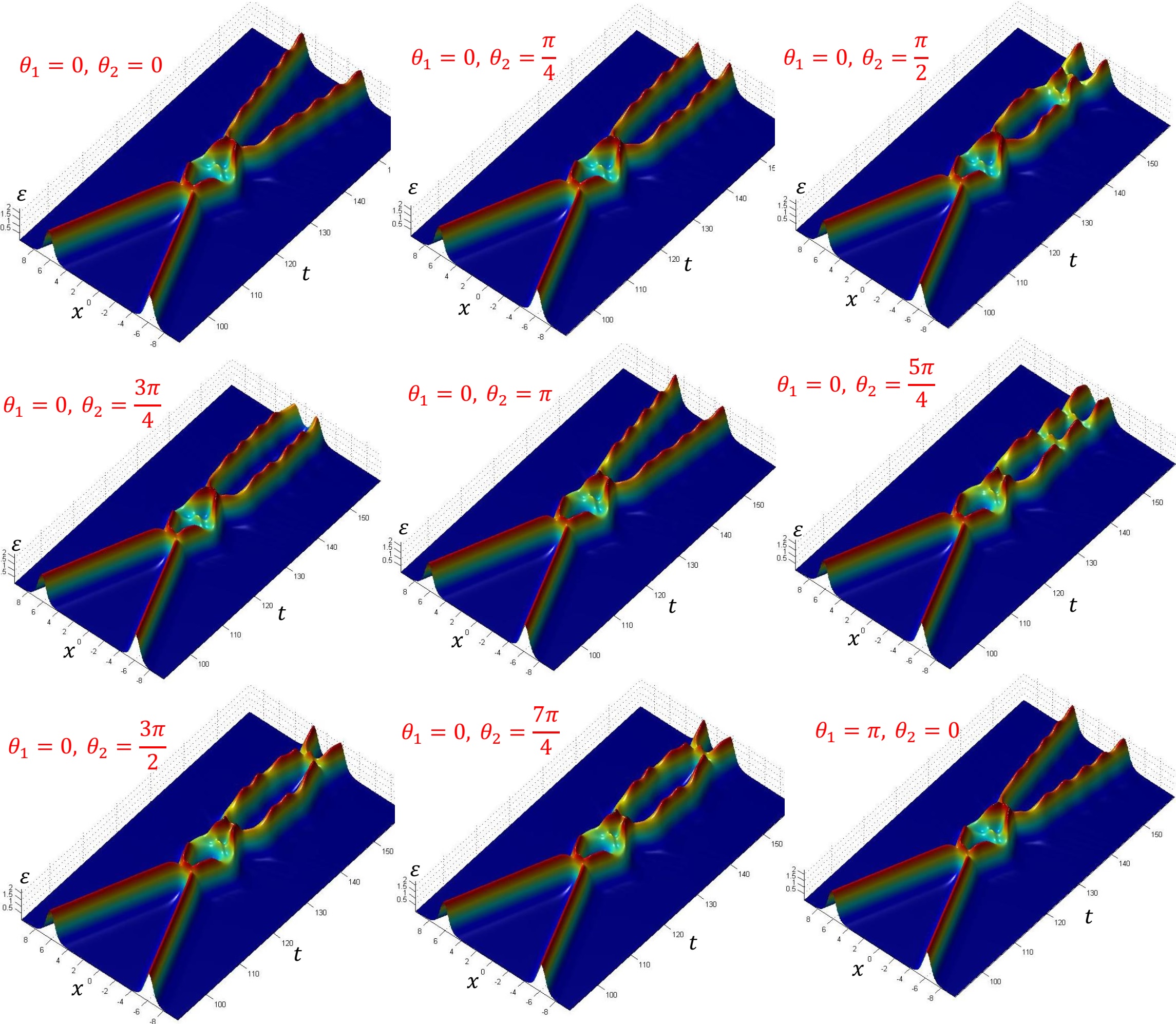
Figure 12: Energy density representations of a disturbed $H_{\{+\}}-V_{\{-\}}$ collision. We have set $v=0.2$, $\alpha=1.5$, $a=-24.5$, $b=24.5$ and $A=0.05$. They show that different initial phases of the trapped wave-packets lead to different fates of the collision.

Moreover, numerically, one can show that there is no difference between undisturbed $H_{\{+\}}-V_{\{+\}}$, $H_{\{+\}}-V_{\{-\}}$, $H_{\{-\}}-V_{\{+\}}$ and $H_{\{-\}}-V_{\{-\}}$ collisions in the energy density representation, i.e. all of them will give the same energy density figures after collisions. But for disturbed ones, it was seen numerically that depending on what type of $H$ and $V$ to use, the resulting energy density figures will be different (see Fig 13).

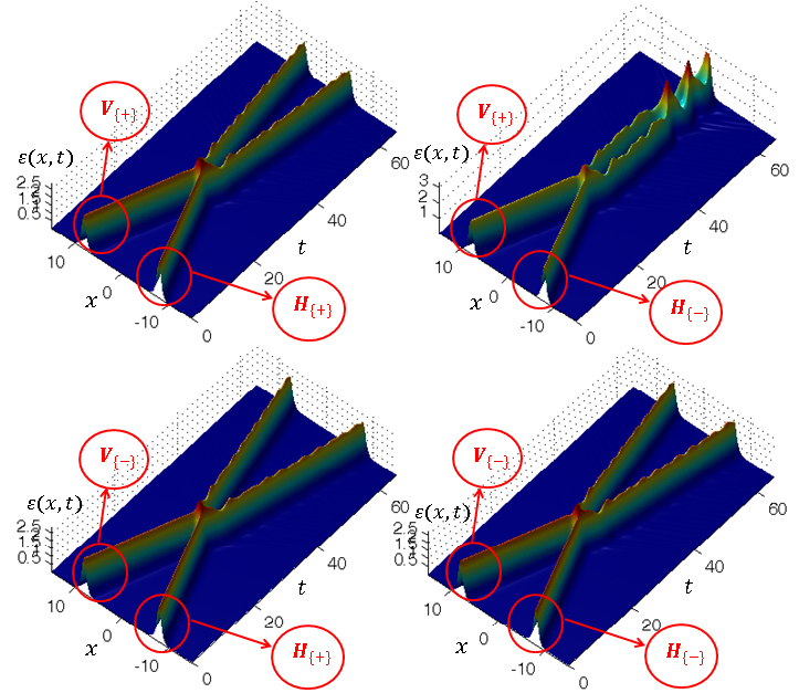
Figure 13: Energy density representations for different type of a disturbed $H-V$ collision with $0.3$ initial speed when $\alpha=1.2$. The initial phases of the trapped wave packets are $\theta_{1}=-\frac{\pi}{3}$ and $\theta_{2}=0$. The same amplitude of the initial small trapped wave packets by $H$ and $V$-solitons have set to $A=0.04$.

To more support, two different situations for disturbed $H_{\{+\}}-V_{\{-\}}$ collisions can be studied. First, for fixing initial phases $\theta_{1}=0$, $\theta_{2}=0$ ($\theta_{2}=\pi$), initial speed $v=0.25$, the same maximum amplitude of the small trapped wave packets $A=0.05$, and initial positions $b=-b=14$, then we can study the collision fates for different $\alpha$’s (see Fig. 14 and Fig. 15). Second, for fixing $\theta_{1}=0$, $\theta_{2}=0$, $A=0.05$, $\alpha=1.2$, and $a=-b=-10$, then we can study the collision fates for different velocities (Fig. 16 and Fig. 17). It is seen numerically that the high speed collisions (energetic collisions) reduce the influence of the initial trapped wave packets in the collision fates, i.e. we do not see significant different fates in the outputs of the energetic collisions (compare Fig. 16 with Fig. 17 for collisions with initial speeds larger than $v=0.4$). Moreover, comparting Fig. 14 with Fig. 15 reveals that the systems for which $\alpha$ are close to 0 or 2, are less affected by the initial trapped wave packets properties.

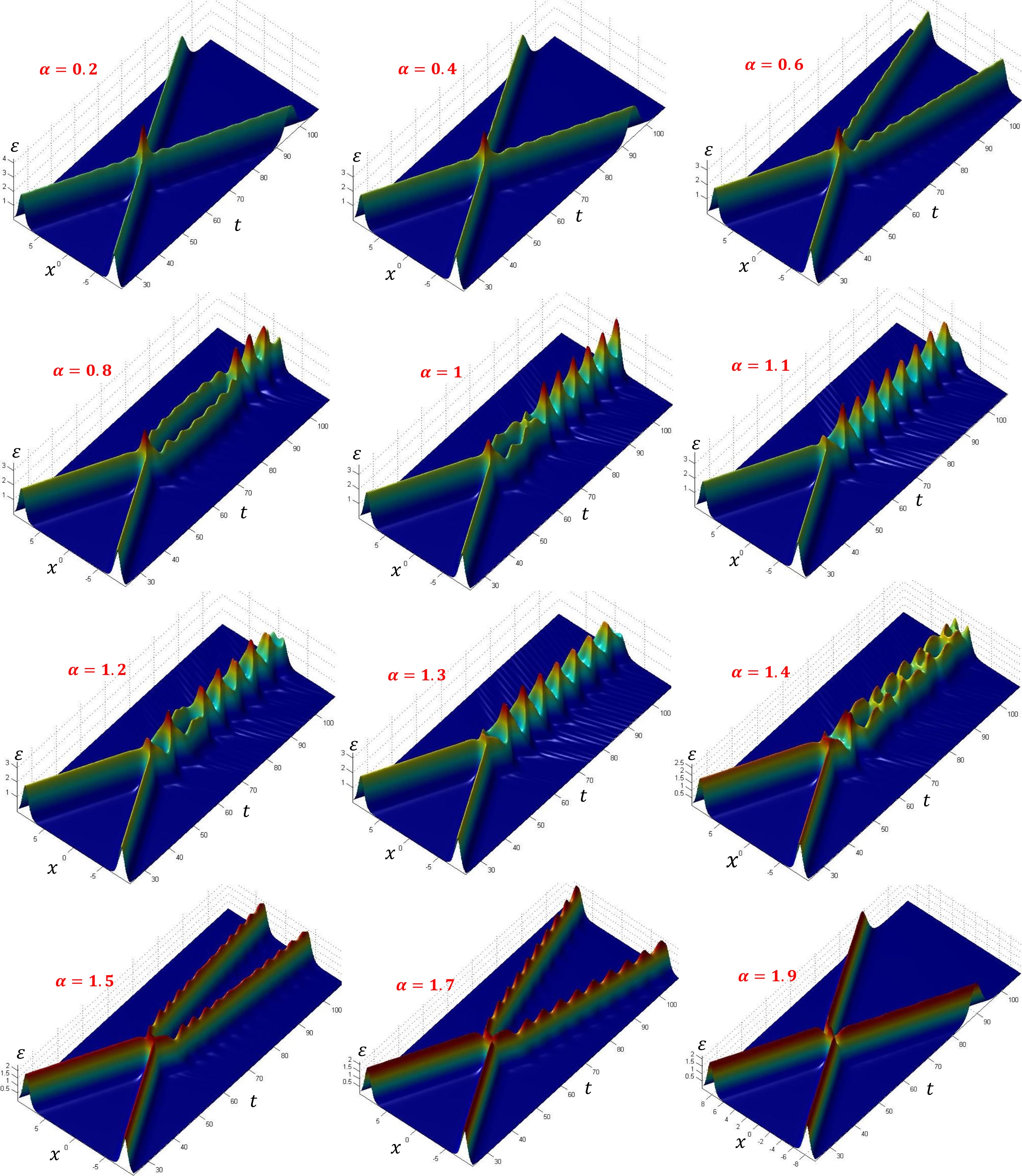
Figure 14: Energy density representations of a disturbed $H_{\{+\}}-V_{\{-\}}$ collision for different $\alpha$’s. We have set $\theta_{1}=0$, $\theta_{2}=0$, $v=0.25$, $b=-a=14$ and $A=0.05$.

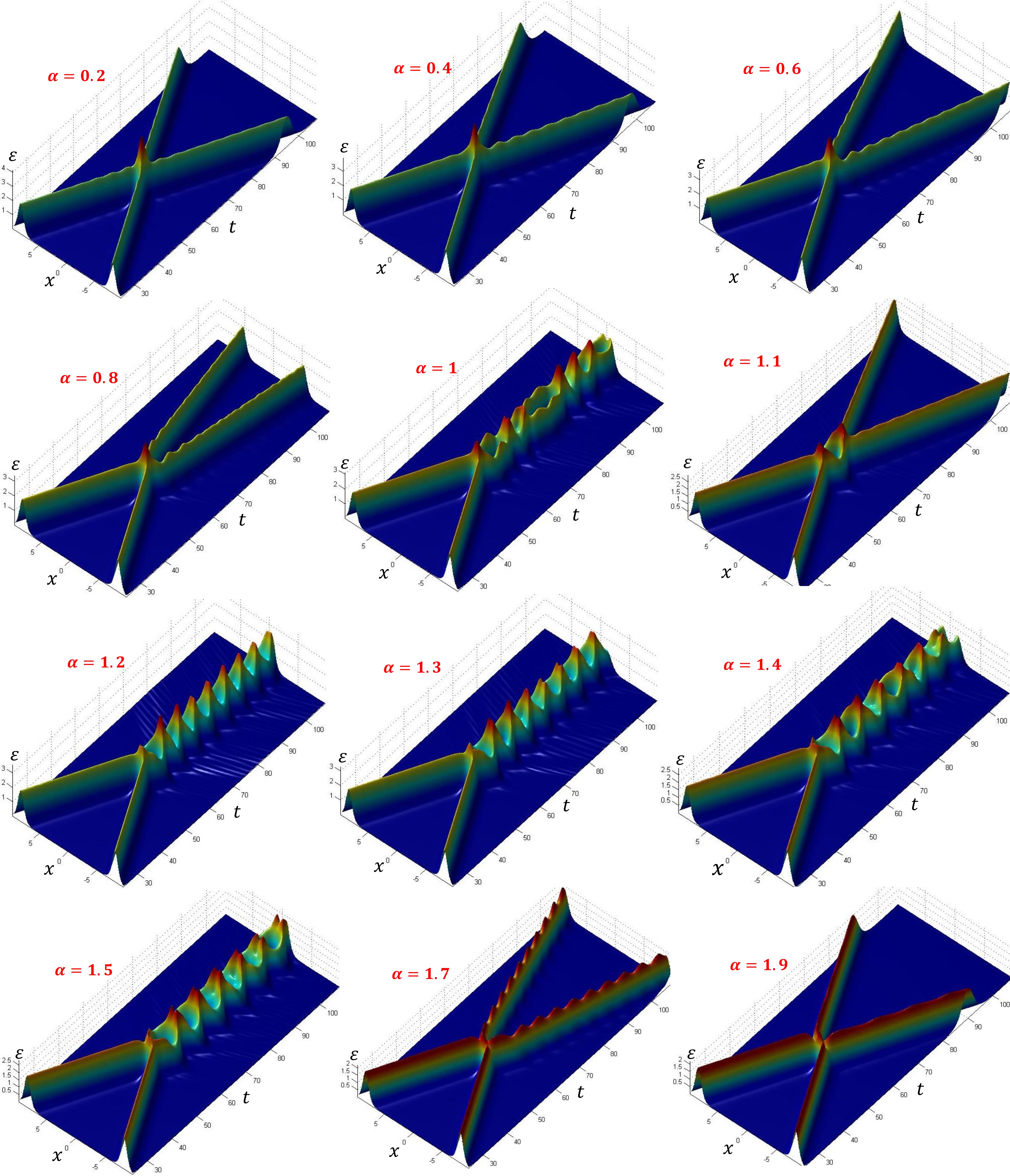
Figure 15: Energy density representations of a disturbed $H_{\{+\}}-V_{\{-\}}$ collision for different $\alpha$’s. We have set $\theta_{1}=0$, $\theta_{2}=\pi$, $v=0.25$, $b=-a=14$ and $A=0.05$.

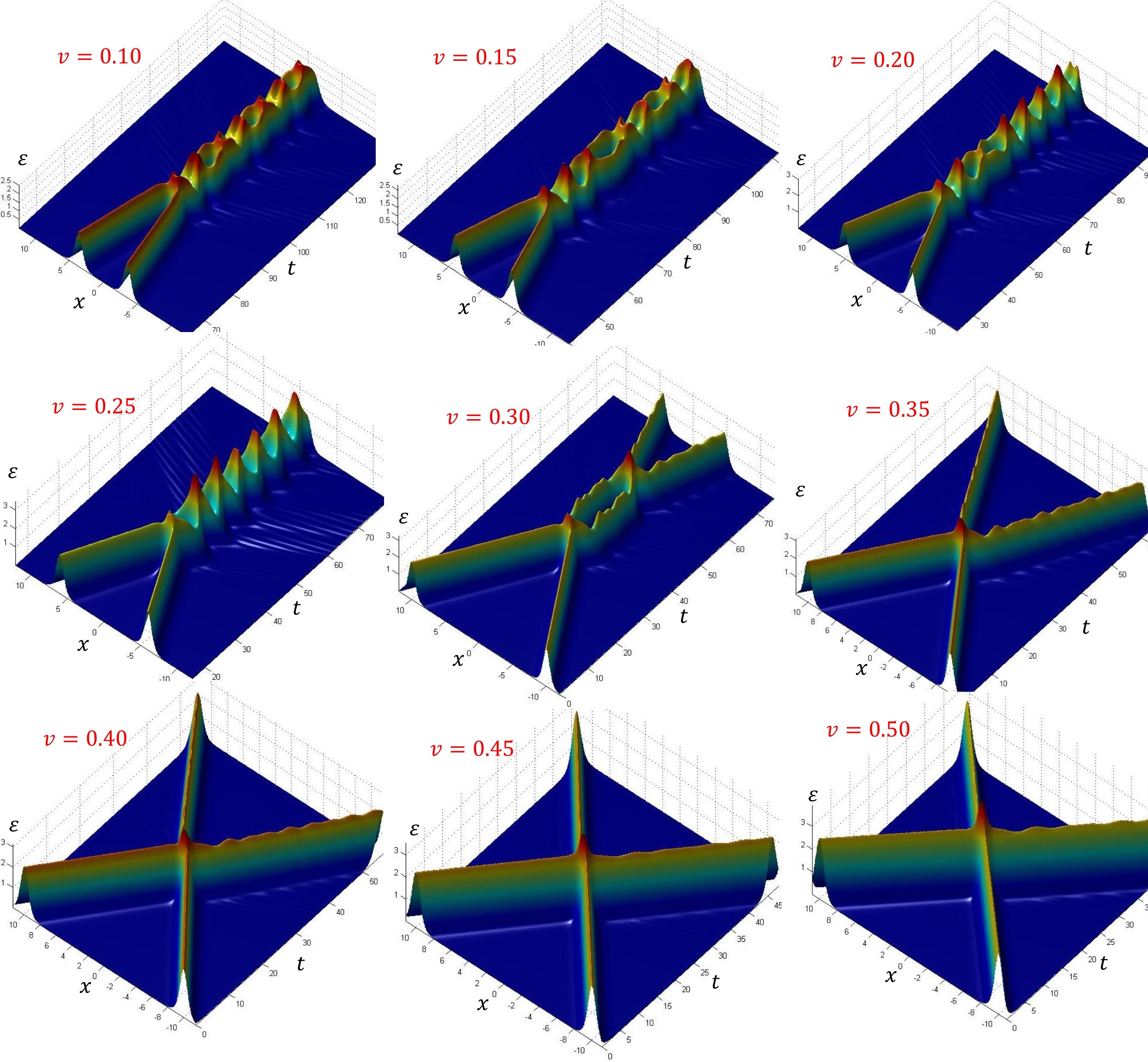
Figure 16: Energy density representations of a disturbed $H_{\{+\}}-V_{\{-\}}$ collision for different velocities. We have set $\alpha=1.2$, $\theta_{1}=0$ and $\theta_{2}=0$, $a=-b=-10$ and $A=0.05$.

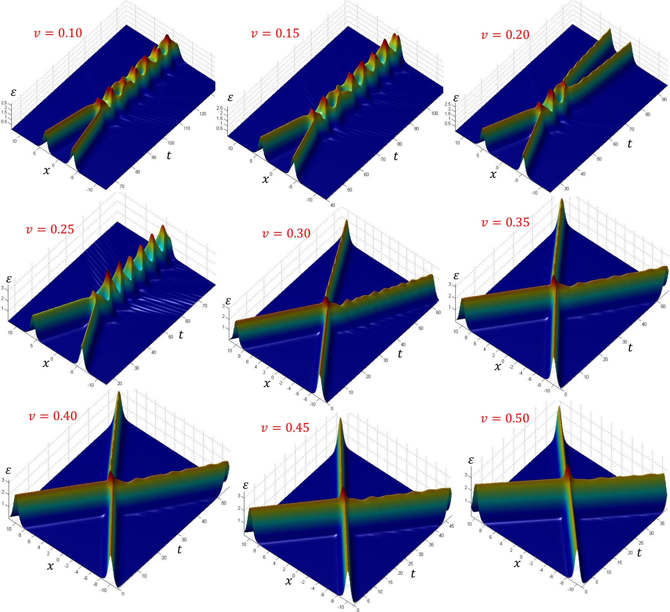
Figure 17: Energy density representations of a disturbed $H_{\{+\}}-V_{\{-\}}$ collision for different velocities. We have set $\alpha=1.2$, $\theta_{1}=0$ and $\theta_{2}=\pi$, $a=-b=-10$ and $A=0.05$.

Therefore, there is an apparent uncertainty in the collision process which originates from the amplitudes and initial phases of the trapped perturbations. The initial phase does not play any crucial role in the particle aspect of a single soliton, but it is the main reason of the uncertainty in collisions, i.e. it can lead to completely different fates. However, for undisturbed solitons there is no uncertainty and everything is predictable. Of course, in real word, random phase perturbation are inevitable, and therefore we might expect probabilistic behaviour in soliton scattering. In fact, the initial phases, in this model, behave like a hidden variable which cause to a probabilistic behaviour for final fates of different particle-like solutions in collision processes.

In this paper, we showed that in general, as seen in the figures, which two solitons capture each other always lead to similar breathing oscillating structures after collisions. However, these breathing oscillating structures have been seen in many different nonlinear systems in $1+1$ and $2+1$ dimensions similarly G ; R1 ; R2 ; MM2 . We think that this similarity, just is referred to the non-linearity nature of them. That is, apparently, the emergence of such structures is a common feature that is related to the nature of the nonlinear systems. But, in general there is not any other meaningful relationship between them. For example, the special cases which were seen in R2 are happened when some special conditions are fulfilled, while there are not such restrictive conditions in our model and other kink-bearing models to see such breathing oscillating structures. Moreover, the kink-bearing systems are essentially relativistic, while the other systems R1 ; R2 are non-relativistic and this is another difference.

VI SUMMERY AND CONCLUSIONS

Inspired by the well-known sine-Gordon (SG) system, we presented a coupled system of the non-linear PDEs which was built by two real scalar fields $\phi$ and $\psi$ in $1+1$ dimensions. A free parameter $\alpha$ was introduced to characterize the coupling provided $\alpha\leqslant 2$. For $\alpha=0$ and $\alpha=2$, we retrieved two independent SG systems. The coupled system was shown to have three different $H$, $V$ and $D$-soliton solutions. $H$ and $V$ solutions are nothing but the known SG kink (anti-kink) solutions for fields $\phi$ and $\psi$ respectively, and $D$ solutions are a composite of $H$ and $V$ solions. It was seen numerically that for systems with $0<\alpha<2$, there are always some permanent small wave packets which are trapped inside solitons after collisions. We classified $H$, $V$ and $D$-solitons with introducing subscripts $\{+\}$ and $\{-\}$ to recognize their topological charges.

It was seen analytically that for systems with $0<\alpha<2$, there is an internal mode for $H$, $V$ and $D$-solitons which makes them able to trap a small wave packet. A wave packet is characterized by an eigenfunction and a special frequency $\omega_{o}$ (or eigenvalue $\omega_{o}^{2}$) of a Schrödinger-like equation. We found numerically that there is an uncertainty in collision fates between disturbed solitons, i.e. the ones which initially trap small wave packets. This uncertainty originates from the amount of the maximum amplitudes and initial phases of the small trapped wave packets by solitons. For different initial phases, particle aspect of the solitons remain unchanged, while the final behaviour may be drastically affected. Nevertheless, the energetic collisions reduce the influence of the initial trapped wave packets on the collision fates. Moreover, the systems for which $\alpha$ are close to 1 or 2 are less affected by the initial trapped wave packets properties.

References

- (1) R. Rajaraman, Solitons and Instantons (North Holland, Elsevier, Amsterdam, 1982).
- (2) A. Das, Integrable Models (World Scientific, 1989).
- (3) G. L. Lamb, Elements of Soliton Theory (Dover Publications, 1995).
- (4) P. G. Drazin and R. S. Johnson, Solitons: an Introduction (Cambridge University Press, 1989).
- (5) N. Riazi, A. Azizi and S. M. Zebarjad, Soliton decay in a coupled system of scalar fields, Phys. Rev. D, 66, 065003 (2002).
- (6) D. Bazeia, R. F. Ribeiro and M. M. Santos, Topological defects inside domain walls, Phys. Rev. D, 54, 1852 (1996).
- (7) D. Bazeia, J.R.S. Nascimento, R.F. Ribeiro and D. Toledo, J. Phys. A, Soliton stability in systems of two real scalar fields, 30, 8157 (1997).
- (8) N. Riazi, M. M. Golshan and K. Mansuri, Coupled systems of scalar fields: stability of quantization of soliton-like solutions, Int. J. Theor. Phys. Group Theor, 7, 91 (2001).
- (9) R. Khomeriki and J. Leon, Bistability in the sine-Gordon equation: The ideal switch, Phys. Rev. E, 71, 056620 (2005).
- (10) L. V. Yakushevich, Nonlinear Physics of DNA (Wiley, 2004).
- (11) L. V. Yakushevich, A. V. Savin and L. I. Manevitch, Nonlinear dynamics of topological solitons in DNA, Phys. Rev. E, 66, 016614 (2002).
- (12) S. Cuenda, A. Sanchez and N. R. Quintero, Does the dynamics of sine–Gordon solitons predict active regions of DNA?, Physica. D, 223, 214 (2006).
- (13) J. Timonen, M. Stirland, D. J. Pilling, Y. Cheng and R. K. Bullough, Statistical Mechanics of the Sine-Gordon Equation, Phys. Rev. Lett, 56, 2233 (1986).
- (14) N. Riazi, Dynamics of solitons in inhomogeneous Josephson junctions, Int. J. Theor. Phys., 35, 101 (1996).
- (15) T.D. Lee, Particle Physics and Introduction to Field Theory (Harwood, 1981).
- (16) N. Riazi, Wave particle duality in non-linear Klein-Gordon equation, Int. J. Theor. Phys, 50, 3451 (2011).
- (17) S. Coleman, New Phenomena in Subnuclear Physics, Ed. by A. Zichichi, (Plenum Press 1977).
- (18) D. K. Campbell, M. Peyrard and P. Sodano, Kink-antikink interactions in double sine-Gordon equation, Physica D, 19, 165 (1986).
- (19) R. H. Goodman and R. Haberman, Kink-Antikink Collisions in the Equation: The n-Bounce Resonance and the Separatrix Map, Siam J. Appl. Dyn. Syst, 4, 1195 (2005).
- (20) O. V. Charkina, Internal Modes of Solitons and Near-Integrable Highly-Dispersive Nonlinear Systems, M. M. Bogdan and B. I. Verkin, Symmetry. Integr. Geom, 2, 047 (2006).
- (21) A. R. Gharaati, N. Riazi and F. Mohebbi, Internal modes of relativistic solitons, Int. J. Theor. Phys, 45, 57 (2006).
- (22) M. Mohammadi and N. Riazi, Approaching integrality in bidimensional nonlinear field equations, Prog. Theor. Phys, 126, 237 (2011).
- (23) O. K. Pashaev, J. H. Lee and C. Rogers, Soliton resonances in a generalized nonlinear Schrödinger equation, J. Phys. A: Math. Theor, 41, 452001(2008).
- (24) K. Sakkaravarthi, T. Kanna, M. Vijayajayanthi, and M. Lakshmanan, Multicomponent long-wave–short-wave resonance interaction system: Bright solitons, energy-sharing collisions, and resonant solitons, Phys. Rev. E, 90, 052912 (2014).
- (25) M. Mohammadi and N. Riazi, Bi-dimensional soliton-like solutions of the non-linear complex sine-Gordon systems, Prog. Theor. Exp. Phys, 2014, 023A03 (2014).