Quantum phases of tilted dipolar bosons in two-dimensional optical lattice

Abstract

We consider a minimal model to describe the quantum phases of ultracold dipolar bosons in two-dimensional (2D) square optical lattices. The model is a variation of the extended Bose-Hubbard model and apt to study the quantum phases arising from the variation in the tilt angle $\displaystyle\theta$ of the dipolar bosons. At low tilt angles $\displaystyle 0^{\circ}\leqslant\theta\apprle 25^{\circ}$, the ground state of the system are phases with checkerboard order, which could be either checkerboard supersolid or checkerboard density wave. For high tilt angles $\displaystyle 55^{\circ}\apprge\theta\apprge 35^{\circ}$, phases with striped order of supersolid or density wave are preferred. In the intermediate domain $\displaystyle 25^{\circ}\apprle\theta\apprle 35^{\circ}$ an emulsion or SF phase intervenes the transition between the checkerboard and striped phases. The attractive interaction dominates for $\displaystyle\theta\apprge 55^{\circ}$, which renders the system unstable and there is a density collapse. For our studies we use Gutzwiller mean-field theory to obtain the quantum phases and the phase boundaries. In addition, we calculate the phase boundaries between an incompressible and a compressible phase of the system by considering second order perturbation analysis of the mean-field theory. The analytical results, where applicable, are in excellent agreement with the numerical results.

I Introduction

In the strongly interacting regime, neutral bosons with short range interactions in optical lattices exhibit two quantum phases: Mott-insulator (MI) and superfluid (SF) Fisher et al. (1989); Jaksch et al. (1998); Greiner et al. (2002a, b). A prototypical model, which describes the properties of such systems is the Bose-Hubbard model (BHM) Fisher et al. (1989); Jaksch et al. (1998); Hubbard (1963). The model considers nearest neighbour hopping and onsite interaction between the bosons. The model is, however, not suitable to describe quantum phases which have offsite density-density correlations, such as, density wave (DW), supersolid (SS) etc Penrose and Onsager (1956); Batrouni and Scalettar (2000); Kim and Chan (2004a, b); Góral et al. (2002); Boninsegni and Prokof’ev (2005); Yi et al. (2007); Danshita and Sá de Melo (2009). The emergence of these quantum phases and their stabilization require long range interactions. The interaction could be dipole-dipole interaction Góral et al. (2002); Yi et al. (2007); Danshita and Sá de Melo (2009); Lahaye et al. (2009); Baranov et al. (2012), fermions mediated boson-boson interaction in Bose-Fermi mixtures Büchler and Blatter (2003), etc. The former is realized in dipolar atoms like Cr Griesmaier et al. (2005); Stuhler et al. (2005); Lahaye et al. (2007), Dy Lu et al. (2011); Tang et al. (2015), Er Aikawa et al. (2012); Baier et al. (2016), and polar molecules Ospelkaus et al. (2006); Danzl et al. (2008); Ni et al. (2008); Ospelkaus et al. (2009); Chotia et al. (2012); Frisch et al. (2015). Apart from quantum phases in optical lattices, dipolar bosons specifically polar molecules, offer fast and robust schemes for quantum computation  Carr et al. (2009); Gorshkov et al. (2011); Hazzard et al. (2014). In addition, the long range and anisotropic nature of the dipole-dipole interaction can induce exotic magnetic orders. Thus, these systems are promising simulators for quantum magnetism Pu et al. (2001); Micheli et al. (2006); Barnett et al. (2006); de Paz et al. (2013).

The BHM with the nearest neighbour (NN) lattice sites inter-particle interaction and its variations are referred to as the extended Bose-Hubbard model (eBHM) Mazzarella et al. (2006); Dutta et al. (2015). It is a minimal model which harbours phases with off site density-density correlations. Based on this model several theoretical studies have analyzed the equilibrium phases of bosons in optical lattices and their stability properties Sengupta et al. (2005); Scarola and Das Sarma (2005); Kovrizhin et al. (2005); Scarola et al. (2006); Menotti et al. (2007); Iskin (2011); Trefzger et al. (2011), and dynamics of the quantum phase transitions by quenching system parameters Shimizu et al. (2018a, b). In 2D this is equivalent to dipole-dipole interaction limited to the NN interaction and with the dipoles aligned perpendicular to the lattice plane. And, such systems exhibit checkerboard order in the DW and SS phases. Thus, a minimal model to describe quantum phases of dipolar bosons in optical lattices is to limit the interaction to NN. This is the system we consider in our present work. In previous studies, the quantum phases of lattice bosons with anisotropic dipolar interaction and their stability has been analyzed Góral et al. (2002); Yi et al. (2007); Danshita and Sá de Melo (2009). In addition, the phase diagrams for the dipolar bosons in 2D square optical lattice with staggered flux in the minimal model has been done Tieleman et al. (2011). A recent work Zhang et al. (2015) reported the equilibrium phases of the hardcore dipolar bosons at half filling in a 2D optical lattice with the variation of tilt angle. And, they reported DW phase with checkerboard and stripe order. However, the experimental observations are in the soft-core regime Baier et al. (2016). In this experiment Baier et al. Baier et al. (2016) have realized the eBHM for the strongly magnetic Er atoms in a 3D optical lattice and observed NN interaction as a genuine consequence of the long-range dipolar interactions. And, they also vary tilt angle of the dipolar atoms to examine the effect of anisotropic dipole-dipole interaction on the SF-MI phase transition.

Motivated by the experimental realization, we investigate the quantum phases of tilted softcore dipolar bosons in a 2D square optical lattice. Hence, our work addresses a key research gap in the physics of softcore dipolar bosons in the strongly interacting domain. We show that the system exhibits compressible checkerboard SS (CBSS) and striped SS (SSS) phases in addition to the incompressible checkerboard DW (CBDW) and striped DW (SDW) phases. Our results can be experimentally examined since tilting the dipoles have become a standard tool box to understand physics of ultracold dipolar bosons and fermions Bismut et al. (2012); Aikawa et al. (2014); Veljić et al. (2018).

We have organized the remainder of this article as follows. In Sec. II we discuss the zero-temperature Hamiltonian of the minimal model. The Sec. III provides a brief account of the Gutzwiller mean-field theory, and the quantum phases of the model. Then, in the later part of the section, we discuss the mean-field decoupling theory to calculate the compressible-incompressible phase boundaries analytically. The Sec. IV describes the numerical procedures adopted to solve the model. The phase diagrams and key results of our work are discussed in Sec. V. We, then, conclude in Sec. VI.

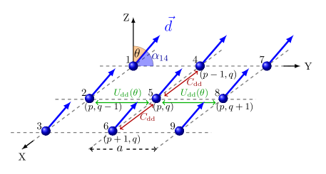
Figure 1: (Color online) Schematics of the dipolar bosons in two dimensional square optical lattice with dipolar interaction among the bosons at nearest-neighbour (NN) lattice sites. We consider the dipoles are polarized in the y-z plane and the angle subtended by the direction of the dipole moments (polarization axis) with the z-axis is the tilt angle $\displaystyle\theta$. The tilt angle is illustrated by the orange colored shaded sector. The angle between the polarization axis and the vector $\displaystyle(\vec{r}_{4}-\vec{r}_{1})$, $\displaystyle\alpha_{14}$, is marked by the blue colored shaded sector. The dipolar interaction between the bosons at lattice sites $\displaystyle(p,q)$ and $\displaystyle(p\pm 1,q)$ is $\displaystyle C_{\rm dd}$, whereas the interaction between the bosons at lattice sites $\displaystyle(p,q)$ and $\displaystyle(p,q\pm 1)$ is $\displaystyle U_{\rm dd}(\theta)=C_{\rm dd}(1-3\sin^{2}\theta)$

II Theoretical Model

We consider charge neutral, polarized dipolar bosons loaded in a 2D square optical lattice with lattice constant $\displaystyle a$. At zero temperature, the physics of such a system is well described by the lowest band Bose-Hubbard model (BHM) with dipolar interaction. The grand canonical Hamiltonian of the system is Fisher et al. (1989); Góral et al. (2002); Boninsegni and Prokof’ev (2005); Yi et al. (2007); Danshita and Sá de Melo (2009):

$$\hat{H}=-J\sum_{\langle ij\rangle}(\hat{b}_{i}^{\dagger}\hat{b}_{j}+{\rm H.c.})-\sum_{i}\mu\hat{n}_{i}+\hat{H}_{I},$$ (1)

where $\displaystyle i\equiv(p,q)$ and $\displaystyle j\equiv(p^{\prime},q^{\prime})$ denote the lattice indices, $\displaystyle\hat{b}_{i}$ ($\displaystyle\hat{b}_{i}^{\dagger}$) and $\displaystyle\hat{n}_{i}$ are bosonic annihilation (creation) and occupation number operators, and $\displaystyle\langle...\rangle$ denotes sum over NN lattice sites. In addition, $\displaystyle J$ and $\displaystyle\mu$ are the strength of the hopping and chemical potential, respectively. The last term is the interatomic interaction Hamiltonian

$$\hat{H}_{I}=\sum_{i}\frac{U}{2}\hat{n}_{i}(\hat{n}_{i}-1)+\frac{C_{\rm dd}}{2}\sum_{ij}\hat{n}_{i}\hat{n}_{j}\frac{(1-3{\rm cos}^{2}\alpha_{ij})}{|\vec{r}_{j}-\vec{r}_{i}|^{3}},$$ (2)

where, $\displaystyle U$ and $\displaystyle C_{\rm dd}\propto d^{2}/a^{3}$ are the strengths of the onsite and dipolar interactions, respectively. Here, $\displaystyle d$ is the magnitude of the induced dipole moment, and $\displaystyle\alpha_{ij}$ is the angle between the polarization axis and the vector $\displaystyle(\vec{r}_{j}-\vec{r}_{i})$. In units of $\displaystyle a$ the position vectors of the lattices $\displaystyle\vec{r}_{i}\equiv(p\hat{e}_{x}+q\hat{e}_{y})$ and $\displaystyle\vec{r}_{j}\equiv(p^{\prime}\hat{e}_{x}+q^{\prime}\hat{e}_{y})$.

In our study, for simplicity, we limit the dipolar interaction to NN sites. Then,

$$\hat{H}_{I}=\sum_{i}\frac{U}{2}\hat{n}_{i}(\hat{n}_{i}-1)+\frac{C_{\rm dd}}{2}\sum_{\langle ij\rangle}\hat{n}_{i}\hat{n}_{j}(1-3{\rm cos}^{2}\alpha_{ij}).$$ (3)

This minimal model is apt for studying the quantum phases of dipolar bosons emerging from the anisotropic nature of the dipolar interaction. In addition, we consider the dipoles are polarized in the $\displaystyle yz$-plane as illustrated in Fig (1), and define the angle between the $\displaystyle z$-axis and polarization axis as the tilt angle $\displaystyle\theta$. With this choice, $\displaystyle\alpha_{ij}$ changes as a function of $\displaystyle\theta$, which can be varied by changing the orientation of the applied magnetic field. Then, the NN interaction along $\displaystyle x$-axis is always repulsive, constant, and independent of $\displaystyle\theta$. Whereas, along the $\displaystyle y$-axis the NN interaction is $\displaystyle U_{\rm dd}(\theta)=C_{\rm dd}(1-3\sin^{2}\theta)$. It varies from $\displaystyle C_{\rm dd}$ to $\displaystyle-2C_{\rm dd}$ as $\displaystyle\theta$ is tuned from $\displaystyle 0^{\circ}$ to $\displaystyle 90^{\circ}$. And, the zero of $\displaystyle U_{\rm dd}(\theta)$ occurs when $\displaystyle\theta=\theta_{\rm M}=\sin^{-1}\big{(}1/\sqrt{3}\big{)}\approx 35.3^{\circ}$. This angle is referred to as the magic angle Ueda (2010) and at this tilt angle the interaction arising from dipolar interaction is absent along the $\displaystyle y$-axis. Thus, the interaction along $\displaystyle y$-axis is repulsive when $\displaystyle\theta<35.3^{\circ}$, and attractive for $\displaystyle\theta>35.3^{\circ}$.

III Theoretical methods

III.1 Gutzwiller mean-field theory

To solve the model, we consider site decoupled mean-field (MF) approximation Fisher et al. (1989); Rokhsar and Kotliar (1991); Sheshadri et al. (1993); Bai et al. (2018); Pal et al. (2019); Suthar et al. (2019). For this, the bosonic annihilation operator of site $\displaystyle(p,q)$, $\displaystyle\hat{b}_{p,q}$, is decomposed to a mean-field $\displaystyle\phi_{p,q}$ and fluctuation operator $\displaystyle\delta\hat{b}_{p,q}$ as $\displaystyle\hat{b}_{p,q}=\langle\hat{b}_{p,q}\rangle+\delta\hat{b}_{p,q}=\phi_{p,q}+\delta\hat{b}_{p,q}$. A similar decomposition is applied to $\displaystyle\hat{b}^{\dagger}_{p,q}$ and $\displaystyle\hat{n}_{p,q}$. It is to be mentioned that, here after we adopt the explicit notation $\displaystyle(p,q)$ to denote a lattice site in 2D. To obtain the MF Hamiltonian, we use the decomposed operators in $\displaystyle\hat{H}$ and neglect the terms which are quadratic in fluctuation operators. Then, the MF Hamiltonian of the system is

$$\displaystyle\hat{H}_{\rm MF} \displaystyle= \displaystyle\sum_{p,q}\Big{\{}-J\left[\left(\hat{b}_{p+1,q}^{\dagger}\phi_{p,q}+\phi^{*}_{p+1,q}\hat{b}_{p,q}-\phi^{*}_{p+1,q}\phi_{p,q}\right)+\left(\hat{b}_{p,q+1}^{\dagger}\phi_{p,q}+\phi^{*}_{p,q+1}\hat{b}_{p,q}-\phi^{*}_{p,q+1}\phi_{p,q}\right)+{\rm H.c.}\right]-\mu\hat{n}_{p,q}$$ (4)

$$\displaystyle+ \displaystyle\frac{U}{2}\hat{n}_{p,q}(\hat{n}_{p,q}-1)+\frac{C_{\rm dd}}{2}\Big{[}\Big{(}\hat{n}_{p+1,q}\langle\hat{n}_{p,q}\rangle+\langle\hat{n}_{p+1,q}\rangle\hat{n}_{p,q}-\langle\hat{n}_{p+1,q}\rangle\langle\hat{n}_{p,q}\rangle\Big{)}+\Big{(}\hat{n}_{p-1,q}\langle\hat{n}_{p,q}\rangle+\langle\hat{n}_{p-1,q}\rangle\hat{n}_{p,q}$$

$$\displaystyle- \displaystyle\langle\hat{n}_{p-1,q}\rangle\langle\hat{n}_{p,q}\rangle\Big{)}\Big{]}+\frac{U_{\rm dd}(\theta)}{2}\Big{[}\Big{(}\hat{n}_{p,q+1}\langle\hat{n}_{p,q}\rangle+\langle\hat{n}_{p,q+1}\rangle\hat{n}_{p,q}-\langle\hat{n}_{p,q+1}\rangle\langle\hat{n}_{p,q}\rangle\Big{)}+\Big{(}\hat{n}_{p,q-1}\langle\hat{n}_{p,q}\rangle+\langle\hat{n}_{p,q-1}\rangle\hat{n}_{p,q}$$

$$\displaystyle- \displaystyle\langle\hat{n}_{p,q-1}\rangle\langle\hat{n}_{p,q}\rangle\Big{)}\Big{]}\Big{\}}.$$

This can be written in terms of single-site Hamiltonians as

$$\hat{H}_{\rm MF}=\sum_{p,q}\hat{h}_{p,q},$$ (5)

where $\displaystyle\hat{h}_{p,q}$ is the single-site Hamiltonian of site $\displaystyle(p,q)$, which can be expressed as

$$\displaystyle\hat{h}_{p,q}= \displaystyle-J\left[\left(\phi_{p+1,q}^{*}\hat{b}_{p,q}+\phi_{p,q+1}^{*}\hat{b}_{p,q}\right)+{\rm H.c.}\right]-\mu\hat{n}_{p,q}$$

$$\displaystyle+\frac{U}{2}\hat{n}_{p,q}(\hat{n}_{p,q}-1)+\frac{C_{\rm dd}}{2}\hat{n}_{p,q}\Big{(}\langle\hat{n}_{p+1,q}\rangle$$

$$\displaystyle+\langle\hat{n}_{p-1,q}\rangle\Big{)}+\frac{U_{\rm dd}(\theta)}{2}\hat{n}_{p,q}\Big{(}\langle\hat{n}_{p,q+1}\rangle+\langle\hat{n}_{p,q-1}\rangle\Big{)},$$

where we have dropped the pure MF terms. These terms shifts the ground state energy and play no role in determining the ground state or the phase diagrams of the system. We can solve the model by diagonalizing the single-site Hamiltonians coupled through the mean-field $\displaystyle\phi_{p,q}$ self consistently. To obtain the ground state of the system, we consider site dependent Gutzwiller ansatz

$$|\Psi_{\rm GW}\rangle=\prod_{p,q}|\psi_{p,q}\rangle=\prod_{p,q}\sum_{n=0}^{(N_{\rm b}-1)}c^{(p,q)}_{n}|n\rangle_{p,q},$$ (7)

where $\displaystyle\{|n\rangle_{p,q}\}$ are the occupation number basis states at site $\displaystyle(p,q)$, $\displaystyle N_{\rm b}$ is the total number of local Fock states used in the computation, and $\displaystyle c^{(p,q)}_{n}$ are complex coefficients of the ground state $\displaystyle|\psi_{p,q}\rangle$. The normalization of $\displaystyle|\Psi_{\rm GW}\rangle$ is ensured by considering site-wise normalization condition

$$\langle\psi_{p,q}|\psi_{p,q}\rangle=\sum_{n=0}^{(N_{\rm b}-1)}|c^{(p,q)}_{n}|^{2}=1.$$ (8)

Then, the mean-field or superfluid order parameter $\displaystyle\phi_{p,q}$ and the average occupancy $\displaystyle n_{p,q}$ at the lattice site $\displaystyle(p,q)$ are

$$\displaystyle\phi_{p,q} \displaystyle= \displaystyle\langle\Psi_{\rm GW}|\hat{b}_{p,q}|\Psi_{\rm GW}\rangle=\sum_{n=1}^{(N_{\rm b}-1)}\sqrt{n}{c^{(p,q)}_{n-1}}^{*}c_{n}^{(p,q)},$$

$$\displaystyle n_{p,q} \displaystyle= \displaystyle\langle\Psi_{\rm GW}|\hat{n}_{p,q}|\Psi_{\rm GW}\rangle=\sum_{n=0}^{(N_{\rm b}-1)}n|c_{n}^{(p,q)}|^{2}.$$ (9)

As the name indicates, $\displaystyle\phi_{p,q}$ is non-zero quantity in the SF phase, and from the definition, it is an indicator of the number fluctuation. Hence, it is a measure of the long range phase coherence in the system. In other words, the SF phase has off diagonal long range order (ODLRO).

III.2 Quantum phases and their characterization

In absence of the dipolar interaction, depending on $\displaystyle J/U$ there are two ground state quantum phases of the system: the superfluid (SF) and Mott-insulator (MI) phases. The key distinction between these two phases is that $\displaystyle\phi_{p,q}$, as mentioned earlier, is finite in SF phase. But, it is zero in the MI phase. In a homogeneous lattice system, density distribution of these two phases is uniform. However, this translational symmetry can be spontaneously broken with long range dipole-dipole interaction. This leads to the emergence of quantum phases which have periodic density modulations, such as, density wave (DW) and supersolid (SS). In other words, the system can exhibit diagonal order. Among the two phases the SS phase, in addition to the diagonal order, has ODLRO. Therefore, the SS phase has non-zero $\displaystyle\phi_{p,q}$, and $\displaystyle n_{p,q}$ has a periodic structure. On the other hand for the DW phase, like in the MI phase, $\displaystyle\phi_{p,q}$ is zero and $\displaystyle n_{p,q}$ is integer. But, unlike MI phase $\displaystyle n_{p,q}$ in DW show spatial pattern. To characterize the diagonal order in DW and SS phases, we compute the static structure factor

$$S(\vec{k})=\frac{1}{N^{2}}\sum_{i,j}e^{{\rm i}\vec{k}.(\vec{r}_{i}-\vec{r}_{j})}\langle\hat{n}_{i}\hat{n}_{j}\rangle,$$ (10)

where $\displaystyle\vec{k}\equiv(k_{x},k_{y})\equiv(k_{x}\hat{e}_{x}+k_{y}\hat{e}_{y})$ is the reciprocal lattice vector (measured in units of $\displaystyle 1/a$), and $\displaystyle N$ is the total number of bosons in the system. In the present study, depending on the tilt angle $\displaystyle\theta$, the system has $\displaystyle n_{p,q}$ which is either checkerboard or striped. The checkerboard order breaks the translational symmetry along both $\displaystyle x$ and $\displaystyle y$ directions, and is characterized by a finite value of $\displaystyle S(\vec{k})$ at the reciprocal lattice site $\displaystyle\vec{k}=(\pi,\pi)$. In the phases having striped pattern, the translational symmetry is broken only along the $\displaystyle x$-direction. And, $\displaystyle S(\vec{k})$ is non-zero only for $\displaystyle\vec{k}=(\pi,0)$. Thus, the structure factors $\displaystyle S(\pi,\pi)$ and $\displaystyle S(\pi,0)$ can be used to characterize the CB and striped phases. Like the MI phase, the DW phase is an incompressible phase of the system; whereas, in the SF and SS phases, the system is compressible. Table (1) summarizes the distinct characteristics of the different possible phases of the considered system.

Quantum phases	$\displaystyle{n}_{p,q}$	$\displaystyle\phi_{p,q}$	$\displaystyle S(\pi,\pi)$	$\displaystyle S(\pi,0)$
Superfluid (SF)	real	$\displaystyle\neq 0$	$\displaystyle 0$	$\displaystyle 0$
Mott-insulator (MI)	integer	$\displaystyle 0$	$\displaystyle 0$	$\displaystyle 0$
Chekerboard supersolid (CBSS)	real	$\displaystyle\neq 0$	$\displaystyle\neq 0$	$\displaystyle 0$
Striped supersolid (SSS)	real	$\displaystyle\neq 0$	$\displaystyle 0$	$\displaystyle\neq 0$
Emulsion supersolid	real	$\displaystyle\neq 0$	$\displaystyle\neq 0$	$\displaystyle\neq 0$
Chekerboard Density wave (CBDW)	integer	$\displaystyle 0$	$\displaystyle\neq 0$	$\displaystyle 0$
Striped Density wave (SDW)	integer	$\displaystyle 0$	$\displaystyle 0$	$\displaystyle\neq 0$
Emulsion Density wave	integer	$\displaystyle 0$	$\displaystyle\neq 0$	$\displaystyle\neq 0$

Table 1: Illustrates characteristics of different quantum phases of the considered system.

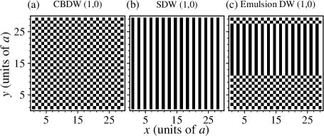
Figure 2: (Color online) Shows the density pattern of the system in distinct density wave phases. Black squares mark those lattice sites which are vacant, and white squares denote singly occupied lattice sites. The states are illustrated for fixed $\displaystyle\mu/J=15$ and $\displaystyle C_{\rm dd}/U=0.8$. The CBDW (1,0) and SDW (1,0) states are obtained for $\displaystyle J/U=0.033$ at $\displaystyle\theta=0^{\circ}$ and $\displaystyle 37^{\circ}$ respectively. The emulsion phase is obtained for $\displaystyle J/U=0.035$ at $\displaystyle\theta=31.5^{\circ}$.

To illustrate the density distribution in the structured phases, the density distribution in the CBDW (1,0), SDW (1,0) and emulsion DW (1,0) are shown in Fig 2. As to be expected, in Fig 2(a) the density modulation of the CBDW (1,0) phase is along both the directions. And, in Fig 2(b) for the SDW (1,0) phase the density modulation is along the $\displaystyle x$-axis. The emulsion phase, as shown in Fig 2(c), has regions with both types of density modulations. And, the simultaneous existence of the two orders is reflected in the non-zero values of the structure factors $\displaystyle S(\pi,\pi)$ and $\displaystyle S(\pi,0)$. The density distribution of the checkerboard, striped and emulsion SS phases are also similar to the density pattern in Fig 2, except the densities are real number.

III.3 Phase boundaries from mean-field decoupling theory

To gain additional insights on the phase transitions between compressible and incompressible phases we calculate the phase boundaries analytically using the mean-field decoupling theory van Oosten et al. (2001); Iskin and Freericks (2009a). A similar analysis can be done using other methods like strong-coupling expansion Freericks and Monien (1996); Iskin and Freericks (2009a); Sachdeva and Ghosh (2012) or random phase approximation Iskin and Freericks (2009b). For this we use the decoupling scheme, described earlier, $\displaystyle\hat{b}_{p,q}=\phi_{p,q}+\delta\hat{b}_{p,q}$, $\displaystyle\hat{b}_{p,q}^{\dagger}=\phi_{p,q}^{*}+\delta\hat{b}_{p,q}^{\dagger}$, and $\displaystyle\hat{n}_{p,q}=n_{p,q}+\delta\hat{n}_{p,q}$. Here, the SF order parameter, $\displaystyle\phi_{p,q}$, is non-zero in SF and SS phases, but zero in the MI and DW phases. Then, assuming the phase transition is continuous, the phase boundary between a compressible ($\displaystyle\phi_{p,q}\neq 0$) and incompressible ($\displaystyle\phi_{p,q}=0$) phase is marked by vanishing SF order parameter $\displaystyle\phi_{p,q}\to 0^{+}$. In addition, the MI and DW phases correspond to integer occupancies per lattice site, and are the exact eigenstates of the interaction and chemical potential part of the mean-field Hamiltonian in Eq. (4). Thus, the hopping term in the Hamiltonian can be considered as a perturbation with $\displaystyle\phi_{p,q}$ as the perturbation parameter. We can, then, perform a perturbative analysis (details are given in Appendix A) to obtain the order parameter from the first order wavefunction as

$$\!\phi_{p,q}=J\overline{\phi}_{p,q}\left[\frac{n_{p,q}+1}{Un_{p,q}-\tilde{\mu}_{p,q}}-\frac{n_{p,q}}{U(n_{p,q}-1)-\tilde{\mu}_{p,q}}\right],$$ (11)

where $\displaystyle\tilde{\mu}_{p,q}=\mu-V^{\rm{dip}}_{p,q}$ and

$$\displaystyle\overline{\phi}_{p,q} \displaystyle= \displaystyle(\phi_{p+1,q}+\phi_{p-1,q}+\phi_{p,q+1}+\phi_{p,q-1}),$$

$$\displaystyle V^{\rm{dip}}_{p,q} \displaystyle= \displaystyle\frac{C_{\rm dd}}{2}(n_{p+1,q}+n_{p-1,q})+\frac{U_{\rm dd}(\theta)}{2}(n_{p,q+1}+n_{p,q-1}).$$

A similar equation is obtained from the Landau procedure for continuous phase transition. In which case the energy functional defined as a function of $\displaystyle\phi_{p,q}$ is minimized Iskin (2011); Sowiński and Chhajlany (2014). In the MI phase, the system has integer commensurate filling, say $\displaystyle n_{0}$, and in the SF phase it has uniform SF order parameter $\displaystyle\varphi_{0}$. With these considerations,

$$\displaystyle\overline{\phi}_{p,q} \displaystyle\equiv \displaystyle\overline{\phi}=4\varphi_{0},$$

$$\displaystyle\tilde{\mu}_{p,q} \displaystyle\equiv \displaystyle\tilde{\mu}=\mu-\left[C_{\rm dd}+U_{\rm dd}(\theta)\right]n_{0}.$$

Since in the SF phase $\displaystyle\varphi_{0}\to 0^{+}$ near the phase boundary, then from Eq. (11) the MI-SF phase boundary can be calculated from

$$\frac{1}{4J}=\left[\frac{n_{0}+1}{Un_{0}-\tilde{\mu}}-\frac{n_{0}}{U(n_{0}-1)-\tilde{\mu}}\right].$$ (12)

The solutions of the above equation defines the MI-SF boundary in the $\displaystyle\mu$-$\displaystyle J$ plane corresponding to the MI lobe with $\displaystyle n_{0}$ filling.

To describe the phase transition from DW to SS phase, we consider two sublattice description of the phases. That is, dipolar interaction induced solid order or spatially periodic modulation can be considered as if the system has two sublattices $\displaystyle A$ and $\displaystyle B$. Each sublattice has different occupancies $\displaystyle n_{A}$ and $\displaystyle n_{B}$ as well as two order parameter $\displaystyle\varphi_{A}$ and $\displaystyle\varphi_{B}$. In the checkerboard order the periodic modulation is along both $\displaystyle x$ and $\displaystyle y$-directions with a period of $\displaystyle 2a$. Whereas, in the striped order the modulation is along one of the directions. So, to obtain the phase boundary between the SDW and SSS phases from Eq. (11), we consider striped sublattice structure. Therefore, we define $\displaystyle\overline{\phi}_{p,q}=2(\varphi_{A}+\varphi_{B})$, $\displaystyle\tilde{\mu}_{A}=\mu-\left[C_{\rm dd}N_{B}+U_{\rm dd}(\theta)N_{A}\right]$ for $\displaystyle(p,q)\in A$ sublattice, and $\displaystyle\overline{\phi}_{p,q}=2(\varphi_{A}+\varphi_{B})$, $\displaystyle\tilde{\mu}_{B}=\mu-\left[C_{\rm dd}N_{A}+U_{\rm dd}(\theta)N_{B}\right]$ for $\displaystyle(p,q)\in B$ sublattice. This leads to two coupled equations for $\displaystyle\varphi_{A}$ and $\displaystyle\varphi_{B}$:

$$\varphi_{A}=2(\varphi_{A}+\varphi_{B})J\left[\frac{n_{A}+1}{Un_{A}-\tilde{\mu}_{A}}-\frac{n_{A}}{U(n_{A}-1)-\tilde{\mu}_{A}}\right],$$ (13a)

$$\varphi_{B}=2(\varphi_{A}+\varphi_{B})J\left[\frac{n_{B}+1}{Un_{B}-\tilde{\mu}_{B}}-\frac{n_{B}}{U(n_{B}-1)-\tilde{\mu}_{B}}\right].$$ (13b)

We solve these two equations simultaneously. In the SSS phase $\displaystyle\{\varphi_{A},\varphi_{B}\}\to 0^{+}$ across the SDW-SSS phase boundary. Then, the SDW-SSS phase boundary is obtained as the solution of

$$\displaystyle\frac{1}{2J}= \displaystyle\left[\frac{n_{A}+1}{Un_{A}-\tilde{\mu}_{A}}-\frac{n_{A}}{U(n_{A}-1)-\tilde{\mu}_{A}}\right]+\left[\frac{n_{B}+1}{Un_{B}-\tilde{\mu}_{B}}\right.$$ (14)

$$\displaystyle\left.-\frac{n_{B}}{U(n_{B}-1)-\tilde{\mu}_{B}}\right].$$

Following similar reasoning, the CBDW-CBSS phase boundary is obtained as the solution of

$$\displaystyle\frac{1}{16J^{2}} \displaystyle= \displaystyle\left[\frac{n_{A}+1}{Un_{A}-\tilde{\mu}_{A}}-\frac{n_{A}}{U(n_{A}-1)-\tilde{\mu}_{A}}\right]$$ (15)

$$\displaystyle\times\left[\frac{n_{B}+1}{Un_{B}-\tilde{\mu}_{B}}-\frac{n_{B}}{U(n_{B}-1)-\tilde{\mu}_{B}}\right].$$

For $\displaystyle\theta=0^{\circ}$, this becomes identical to the phase boundary in 2D reported by Iskin Iskin (2011). The detailed steps of derivations to obtain the above equation are discussed in Appendix (B).

It is to be mentioned here that close to $\displaystyle\theta_{\rm M}$, the system undergoes a checkerboard-striped transition. So, in this regime the system can exhibit both the orders simultaneously, leading to an emulsion DW phase. The parameter domains of such emulsion DW phases are identified as the regions where Eq. (14) and Eq. (15) both applicable.

IV Numerical methods

To obtain the equilibrium phase diagrams of the system, we diagonalize the single-site Hamiltonian in Eq. (LABEL:bhm_hamil_explicit) Bai et al. (2018); Pal et al. (2019). For this, we consider a guess solution of the ground state $\displaystyle|\Psi_{\rm GW}\rangle$ to compute the initial values of $\displaystyle\phi_{p,q}$ and $\displaystyle\langle\hat{n}_{p,q}\rangle$. We then use these values in Eq. (LABEL:bhm_hamil_explicit), and diagonalize it to obtain a new ground state $\displaystyle|\psi_{p,q}\rangle$. Using this new state we update $\displaystyle|\Psi_{\rm GW}\rangle$, and then, compute the corresponding $\displaystyle\phi_{p,q}$ and $\displaystyle\langle\hat{n}_{p,q}\rangle$. We, then, repeat the same for the next lattice site. This is repeated till all the lattices sites are covered. One such step constitutes an iteration, and the iteration is repeated till $\displaystyle\phi_{p,q}$ and $\displaystyle\langle\hat{n}_{p,q}\rangle$ converge. Around the phase boundary the convergence is slow and this is remedied by considering larger number of iterations. To model an uniform infinite size lattice, we perform the above procedure on the surface of a torus by considering periodic boundary conditions along the $\displaystyle x$ and $\displaystyle y$-directions of the finite sized lattice system. In general, we have considered $\displaystyle 12\times 12$ lattice system and $\displaystyle N_{\rm b}=20$ to obtain the phase diagrams. System size dependence of phase boundary occurs when there is an intervening emulsion phase between two phases. For such special cases, we supplement the results from $\displaystyle 12\times 12$ lattice with the results obtained for $\displaystyle 20\times 20$ and $\displaystyle 30\times 30$ lattice systems.

V Results and discussions

The model Hamiltonian considered has five independent parameters, namely, $\displaystyle J$, $\displaystyle U$, $\displaystyle\mu$, $\displaystyle C_{\rm dd}$, and $\displaystyle\theta$. To examine the phase diagram of the system in detail we scale the Hamiltonian with respect to $\displaystyle J$ and set $\displaystyle\mu/J=15$. This reduces the number of independent parameters to three, $\displaystyle U/J$, $\displaystyle C_{\rm dd}/J$ and $\displaystyle\theta$. For better description, we obtain the phase diagrams in the $\displaystyle J/U$-$\displaystyle C_{\rm dd}/U$ plane for different values of $\displaystyle\theta$. This choice is suitable to probe the interplay between the onsite and dipolar interactions in determining the distinct phases of the system.

V.1 $\displaystyle J/U$-$\displaystyle C_{\rm dd}/U$ phase diagrams

The $\displaystyle J/U$-$\displaystyle C_{\rm dd}/U$ phase diagrams for different values of $\displaystyle\theta$ are shown in Fig. (3). In the figure, the solid lines correspond phase boundaries obtained from the Gutzwiller mean-field theory. The filled circles mark the phase boundaries between an incompressible and a compressible phase, which are calculated from the mean-field decoupling theory. From the figure, it is evident that the mean-field decoupling theory, when applicable, gives results which are in good agreement with the Gutzwiller mean-field theory. For the parameters considered we obtain MI phase with unit filling. The MI-SF phase boundary is obtained by solving Eq. (12) with $\displaystyle n_{0}=1$. The SSS-SDW phase boundaries are calculated by solving Eq. (14) with $\displaystyle n_{A}=1$ and $\displaystyle n_{B}=0$ for the SDW (1,0)-SSS boundary, and $\displaystyle n_{A}=2$ and $\displaystyle n_{B}=0$ for the SDW (2,0)-SSS boundary. Similarly, the CBSS-CBDW phase boundaries are calculated by solving Eq. (15) with $\displaystyle n_{A}=1$ and $\displaystyle n_{B}=0$ for the CBDW (1,0)-CBSS boundary, and $\displaystyle n_{A}=2$ and $\displaystyle n_{B}=0$ for the CBDW (2,0)-CBSS boundary.

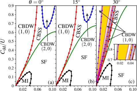
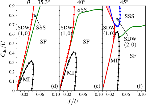
Figure 3: (Color online) Shows the phase diagrams in the $\displaystyle J/U-C_{\rm dd}/U$ plane for different values of the tilt angle $\displaystyle\theta$. The phase diagrams are obtained for $\displaystyle\mu/J=15$. The solid phase boundaries are obtained from the self-consistent numerical diagonalization of mean-field Hamiltonian of the system. Whereas, filled circles mark the phase boundaries between an incompressible and a compressible phase of the system, which are obtained analytically considering perturbation analysis of the mean-field decoupling theory. In Fig. (c), the parameter regions for emulsion SS and emulsion DW (1,0) phases are shaded by silver and gold colors respectively. In these emulsion phases, the system simultaneously exhibits both the orders, checkerboard and striped. The parameter region shaded by pink color in Fig (f) is for the emulsion phase of SDW (1,0) and SDW (2,0) phases.

V.1.1 $\displaystyle\theta=0^{\circ}$,$\displaystyle 15^{\circ}$, and $\displaystyle 30^{\circ}$

The phase diagrams for $\displaystyle\theta=0^{\circ}$, $\displaystyle 15^{\circ}$ and $\displaystyle 30^{\circ}$ are shown in Fig. (3)(a) to (3)(c). These are representative cases for tilt angle lower than the magic angle, that is, $\displaystyle\theta<35.3^{\circ}$. For these $\displaystyle\theta$, $\displaystyle U_{\rm dd}$ is repulsive along both $\displaystyle x$ and $\displaystyle y$-directions. The interaction is isotropic when $\displaystyle\theta=0^{\circ}$, and along $\displaystyle y$-axis interaction strength decreases with the increase of $\displaystyle\theta$. For lower values of $\displaystyle C_{\rm dd}/U$ the system is in DW or SF or MI phase for all values of $\displaystyle\theta$. Out of these, the MI and SF phases do not have diagonal order. But, for higher values of $\displaystyle C_{\rm dd}/U$ the system favors phases with diagonal order. And, we also get CBSS phase in which the system exhibits ODLRO in addition to the diagonal order. In addition, there are domains in the phase diagram where CBDW phases with different filling exist.

In the DW phases ODLRO is absent and the system has only diagonal order. By comparing the phase diagrams shown in Fig. (3)(a) to (3)(c), we can infer that the domain with checkerboard order diminishes with the increase in $\displaystyle\theta$. This is due to the decrease in $\displaystyle U_{\rm dd}$, which increases the anisotropy of the dipolar interaction and checkerboard order becomes energetically unfavourable. At $\displaystyle\theta=30^{\circ}$, Fig. (3)(c), we get metastable emulsion SS and DW phases. The parameter domains of these phases are shaded by the silver and gold colors respectively. In the emulsion phase, the checkerboard and striped orders coexist. The emergence of the emulsion phase at this tilt angle, implies that $\displaystyle U_{\rm dd}$ is weak and cannot support checkerboard order. The system has entered the parameter domain where the striped order has lower energy. Indeed, at lower $\displaystyle\theta$ we obtain phases with striped order. In addition, an important aspect of the phase diagram at $\displaystyle\theta=30^{\circ}$ is the absence of the DW (2,0) phase. It is also to be highlighted that, for this $\displaystyle\theta$, the presence of the emulsion phase renders the mean-field decoupled theory inapplicable to identify phase boundaries between incompressible and compressible phases with diagonal order. This is due to the lack of a well defined unperturbed ground state for the emulsion phase. However, the presence of the emulsion phase can be identified as the domains where Eq. (14) and Eq. (15) indicate simultaneous presence of striped and checkerboard order in the DW (1,0) phase. This overlap region is indicated by the violet filled circles and coincides with the numerical phase boundary between emulsion SS and emulsion DW (1,0) phase. But, this is to be contrasted with the Gutzwiller mean-field results, since within this region we obtain a narrow region of CBDW (1,0) phase surrounded by the regions of emulsion DW (1,0) phase. It is to be mentioned here that the phase diagram for $\displaystyle\theta=0^{\circ}$, shown in Fig. (3)(a), are consistent with the results reported in our previous work Suthar et al. (2019). In our previous work, we had explored the phase diagram of the extended BHM model in the $\displaystyle J/U$-$\displaystyle\mu/U$ plane. And, thus, parts of the phase diagram for specific values of $\displaystyle C_{\rm dd}/U$ and $\displaystyle\mu/J$ in Fig. (3)(a) corresponds to horizontal cuts of the phase diagram reported in ref. Suthar et al. (2019).

V.1.2 $\displaystyle\theta=35.3^{\circ}$ and $\displaystyle 40^{\circ}$

At the magic angle, that is, $\displaystyle\theta=\theta_{\rm M}\approx 35.3^{\circ}$, as mentioned earlier, the dipolar interaction along $\displaystyle y$-axis vanishes. But, the interaction along $\displaystyle x$-axis remains positive and unchanged. Energetically, this favours striped order for the phases with diagonal order. And, as shown in Fig. (3)(d), the phase diagram supports SSS and SDW phases. For $\displaystyle\theta>\theta_{\rm M}$, the dipolar interaction along $\displaystyle y$-axis is attractive. This further enhances the striped phases, and this is discernible from the phase diagram at $\displaystyle\theta=40^{\circ}$ shown in Fig. 3(e). In this case, the SSS phase extends up to $\displaystyle J/U\approx 0.2$ for $\displaystyle C_{\rm dd}/U\approx 0.9$.

V.1.3 $\displaystyle\theta=45^{\circ}$

At higher $\displaystyle\theta$, new stripe phases emerge in the phase diagram, and as an example we examine the phase diagram at $\displaystyle\theta=45^{\circ}$. As shown in Fig. 3(f), SDW (2,0) phase is present in the system when $\displaystyle\theta=45^{\circ}$. However, at lower $\displaystyle\theta$, the stronger attractive interaction along $\displaystyle y$-axis results in the instability of the system and ultimately leads to density collapse. The phase diagram at $\displaystyle\theta=45^{\circ}$ shows two distinct signatures of the onset of the instability. First, the mixing of different phases SDW (1,0) and SDW (2,0) in the domain shaded by pink color. And, second, the merging of different phases MI, SF, SSS and SDW. In contrast, at lower $\displaystyle\theta$ the incompressible phases are separated by an intervening compressible phase. It must be mentioned here that, merging of incompressible phases is also discussed in previous works on 2D BHM with three-body attractive interaction  Safavi-Naini et al. (2012); Singh et al. (2018). The presence of the emulsion phase indicates that the phase transition between SDW (1,0) and SDW (2,0) phases is not second-order. A detail analysis is essential to understand whether the phase transition is first order or a micro-emulsion phase intervenes the phases Spivak and Kivelson (2004).

In the phase diagram there is a triple point of MI, SDW (1,0) and SSS phases at approximately $\displaystyle(0.027,0.5)$. Starting from the triple point there is a sharp phase boundary between the MI phase with unit filling and the SDW (1,0) phase in the range $\displaystyle 0.38\leqslant C_{\rm dd}/U\leqslant 0.50$ and $\displaystyle 0.021\apprle J/U\apprle 0.027$. This phase boundary can either be a first-order phase transition, or a thin region of metastable emulsion of the two phases could possibly exist which is not detectable with the present method. However, for $\displaystyle J/U<0.021$ and $\displaystyle C_{\rm dd}/U<0.38$, we do obtain a very narrow region of the emulsion phase separating these two phases.

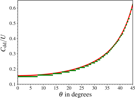
Figure 4: (Color online) Shows the $\displaystyle C_{\rm dd}/U$ value of the tip of the MI lobe as the tilt angle $\displaystyle\theta$ is changed. Green filled circles are obtained from Gutzwiller mean-field theory and solid red line is obtained from Eq. (12).

V.1.4 MI lobe enhancement

One feature of the MI lobe discernible from the phase diagrams in Fig. (3) is its enhancement along the $\displaystyle C_{\rm dd}/U$-axis with increasing $\displaystyle\theta$. To illustrate this, the $\displaystyle\theta$ dependence of the MI lobe tip, in terms of $\displaystyle C_{\rm dd}/U$, is shown in Fig. (4). To analyze this consider the Eq. (12) which defines the MI-SF boundary in the mean-field decoupling theory and rewrite it as

$$\frac{U}{4J}=\left[\frac{n_{0}+1}{n_{0}-\tilde{\mu}/U}-\frac{n_{0}}{(n_{0}-1)-\tilde{\mu}/U}\right].$$ (16)

In absence of the dipolar interaction ($\displaystyle C_{\rm dd}=0$) $\displaystyle\tilde{\mu}=\mu$ and we obtain the MI-SF boundary of the BHM. However, the dipolar interaction reduces the effective chemical potential to $\displaystyle\tilde{\mu}=\mu-C_{\rm dd}(2-3\sin^{2}\theta)$. At $\displaystyle\theta=0^{\circ}$, $\displaystyle\tilde{\mu}$ has the smallest value $\displaystyle\tilde{\mu}_{\rm min}=\mu-2C_{\rm dd}$ and this can be considered as the value of $\displaystyle\tilde{\mu}$ to define the MI-SF boundary. But, when $\displaystyle\theta>0^{\circ}$ the prefactor $\displaystyle(2-3\sin^{2}\theta)$ decreases and hence, to maintain the same value of $\displaystyle\tilde{\mu}$ the strength of the dipolar interaction $\displaystyle C_{\rm dd}$ has to increase. Thus, there is an enhancement of the MI lobe along the $\displaystyle C_{\rm dd}/U$-axis. As the degree of enhancement depends on the prefactor with $\displaystyle\sin^{2}\theta$, the trend noticeable in Fig. (4) is indicative of this dependence. This is consistent with the experimental finding in  Baier et al. (2016), where onsite repulsive dipolar interaction is observed to favour the MI phase due to stronger pinning of the lattice bosons.

V.2 Phase diagrams in $\displaystyle J/U-\theta$ plane

From the phase diagrams in Fig. (3), it is evident that the phase structure is richer with stronger dipolar interaction (large $\displaystyle C_{\rm dd}/U$). Most importantly, the checkerboard order of the system transforms into striped order below a certain value of $\displaystyle\theta$. This is an example of structural phase transition. To examine the phases of the system as a function of $\displaystyle\theta$ we examine the phase diagram in the $\displaystyle J/U-\theta$ plane for fixed values of $\displaystyle C_{\rm dd}/U$ and $\displaystyle\mu/J$. And, as an example the phase diagram for the case of $\displaystyle C_{\rm dd}/U=0.8$ and $\displaystyle\mu/J=15$ is shown in Fig (5).

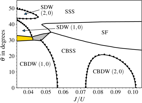
Figure 5: (Color online) Shows the phase diagram in the $\displaystyle J/U-\theta$ plane for $\displaystyle C_{\rm dd}/U=0.8$ and $\displaystyle\mu/J=15$. The solid phase boundaries are obtained from the numerical computation of the Gutzwiller mean-field theory. The filled circles mark the phase boundaries between an incompressible and a compressible phase which are calculated analytically by performing perturbation analysis of the mean-field decoupling theory. The parameter domains shaded by silver and gold colors are for emulsion SS and emulsion DW (1,0) phases respectively. In these emulsion phases, checkerboard and striped order coexist in the system.

Consistent with the phase diagrams in Fig. (3), checkerboard and striped orders are preferred for $\displaystyle\theta\apprle 25^{\circ}$ and $\displaystyle\theta\apprge 35^{\circ}$, respectively. For $\displaystyle 25^{\circ}\apprle\theta\apprle 35^{\circ}$ emulsion phase is the preferred one in the strongly interacting domain. However, in the weakly interacting domain, $\displaystyle J/U\apprge 0.053$, SF phase is the intervening phase between the checkerboard and striped supersolids. These are in good agreement with the previous findings on phase transition between CBDW (1,0) to SDW (1,0) in the hardcore limit of the model Zhang et al. (2015). The intervening emulsion and SF phases implies that there is no sharp phase transition between the two structured phases. And, also it cannot be a second order phase transition in the strongly interacting domain, $\displaystyle J/U\apprle 0.053$. In this domain, the phase transition can either be first order or “Spivak-Kivelson” type phase transition in which a micro-emulsion phase intervenes between two ordered phases Spivak and Kivelson (2004). Considering that the checkerboard order disappears at $\displaystyle\theta$ smaller than the magic angle, implies that it is a delicate phase. It is unstable against large anisotropy of the interaction potential.

An important observation, manifest in Fig. (5), is the parameter domain of the CBDW (2,0) and SDW (2,0) phases. The former occurs in the domain of large $\displaystyle J/U$ and small $\displaystyle\theta$. The later, on the other hand, occurs in the domain with small $\displaystyle J/U$ and large $\displaystyle\theta$. This is, however, due to the choice of $\displaystyle C_{\rm dd}/U$ and $\displaystyle\mu/J$. For a different choice of these two parameters, there could be an intervening emulsion phase for the transition between these two structured phases.

VI Conclusions

In conclusion, we have explored the rich phase structure of soft core dipolar bosons in a 2D optical lattices as a function of tilt angle $\displaystyle\theta$. The key point is that the variation of $\displaystyle\theta$ modifies the anisotropy of the dipolar interaction in the plane of the 2D lattice. And, this leads to the formation of two types of quantum phases with different diagonal orders: checkerboard and striped. Our results indicate that the quantum phase transition between these orders, namely, the checkerboard and stripe orders, occurs through an intervening emulsion phase. The striped order phases, both density wave and supersolid phases, are preferred at high values of $\displaystyle\theta$ when the anisotropy is large. However, above the magic angle $\displaystyle\theta_{\rm M}\approx 35.3^{\circ}$, as the interaction along $\displaystyle y$-axis turns negative, a density instability manifest in the system.

Appendix A Perturbative treatment of SF order parameter

We consider the hopping term in the single-site Hamiltonian as the perturbation and the interaction terms along with the chemical potential as the unperturbed Hamiltonian. Therefore, the energy of the ground state of the unperturbed Hamiltonian

$$\displaystyle E^{0}_{n_{p,q}} \displaystyle= \displaystyle\frac{U}{2}n_{p,q}(n_{p,q}-1)+\frac{C_{\rm dd}}{2}n_{p,q}(n_{p+1,q}+n_{p-1,q})$$ (17)

$$\displaystyle+\frac{U_{\rm dd}(\theta)}{2}n_{p,q}(n_{p,q+1}+n_{p,q-1})-\mu n_{p,q}.$$

Then, to first order in SF order parameter, the perturbed ground state can be written as

$$\displaystyle|\psi_{p,q}\rangle=|n\rangle_{p,q}+\sum_{m\neq n}\frac{{}_{p,q}\langle m|\hat{T}_{p,q}|n\rangle_{p,q}}{E^{0}_{n_{p,q}}-E^{0}_{m_{p,q}}}|m\rangle_{p,q},$$ (18)

where considering the SF order parameter a real number

$$\displaystyle\hat{T}_{p,q} \displaystyle= \displaystyle-J(\phi_{p+1,q}+\phi_{p-1,q}+\phi_{p,q+1}+\phi_{p,q-1})(\hat{b}_{p,q}+\hat{b}^{\dagger}_{p,q})$$ (19)

$$\displaystyle= \displaystyle-J\overline{\phi}_{p,q}(\hat{b}_{p,q}+\hat{b}^{\dagger}_{p,q}).$$

Therefore, using Eqs. (17)- (19) the ground state can be calculated as

$$\displaystyle|\psi_{p,q}\rangle \displaystyle= \displaystyle|n\rangle_{p,q}+J\overline{\phi}_{p,q}\left[\frac{\sqrt{n_{p,q}+1}}{Un_{p,q}-\tilde{\mu}_{p,q}}|n_{p,q}+1\rangle\right.$$ (20)

$$\displaystyle\left.-\frac{\sqrt{n_{p,q}}}{U(n_{p,q}-1)-\tilde{\mu}_{p,q}}|n_{p,q}-1\rangle\right],$$

From this state, we obtain the SF order parameter $\displaystyle\phi_{p,q}$ in the form mentioned in Eq. (11).

Appendix B CBDW-CBSS phase boundary

To obtain the phase boundaries between the CBDW and CBSS phases from Eq. (11), we consider checkerboard sublattice structure. Then, define $\displaystyle\overline{\phi}_{p,q}=4\varphi_{B}$ and $\displaystyle\tilde{\mu}_{A}=\mu-\left[C_{\rm dd}+U_{\rm dd}(\theta)\right]n_{B}$ for $\displaystyle(p,q)\in A$ sublattice, and $\displaystyle\overline{\phi}_{p,q}=4\varphi_{A}$, $\displaystyle\tilde{\mu}_{B}=\mu-\left[C_{\rm dd}+U_{\rm dd}(\theta)\right]n_{A}$ for $\displaystyle(p,q)\in B$ sublattice. This leads to two coupled equations

$$\varphi_{A}=4J\varphi_{B}\left[\frac{n_{A}+1}{Un_{A}-\tilde{\mu}_{A}}-\frac{n_{A}}{U(n_{A}-1)-\tilde{\mu}_{A}}\right],$$ (21a)

$$\varphi_{B}=4J\varphi_{A}\left[\frac{n_{B}+1}{Un_{B}-\tilde{\mu}_{B}}-\frac{n_{B}}{U(n_{B}-1)-\tilde{\mu}_{B}}\right].$$ (21b)

These two equations can be solved simultaneously. In the CBSS phase $\displaystyle\{\varphi_{A},\varphi_{B}\}\to 0^{+}$ across the CBDW-CBSS phase boundary. Then, the CBDW-CBSS phase boundary is obtained as in Eq. (15).

References

- Fisher et al. (1989) M. P. A. Fisher, P. B. Weichman, G. Grinstein, and D. S. Fisher, Phys. Rev. B 40, 546 (1989).
- Jaksch et al. (1998) D. Jaksch, C. Bruder, J. I. Cirac, C. W. Gardiner, and P. Zoller, Phys. Rev. Lett. 81, 3108 (1998).
- Greiner et al. (2002a) M. Greiner, O. Mandel, T. Esslinger, T. W. Hänsch, and I. Bloch, Nature (London) 415, 39 (2002a).
- Greiner et al. (2002b) M. Greiner, O. Mandel, T. W. Hänsch, and I. Bloch, Nature 419, 51 (2002b).
- Hubbard (1963) J. Hubbard, Proc. Royal Soc. A 276, 238 (1963).
- Penrose and Onsager (1956) O. Penrose and L. Onsager, Phys. Rev. 104, 576 (1956).
- Batrouni and Scalettar (2000) G. G. Batrouni and R. T. Scalettar, Phys. Rev. Lett. 84, 1599 (2000).
- Kim and Chan (2004a) E. Kim and M. H. W. Chan, Nature 427, 225 EP (2004a).
- Kim and Chan (2004b) E. Kim and M. H. W. Chan, Science 305, 1941 (2004b).
- Góral et al. (2002) K. Góral, L. Santos, and M. Lewenstein, Phys. Rev. Lett. 88, 170406 (2002).
- Boninsegni and Prokof’ev (2005) M. Boninsegni and N. Prokof’ev, Phys. Rev. Lett. 95, 237204 (2005).
- Yi et al. (2007) S. Yi, T. Li, and C. P. Sun, Phys. Rev. Lett. 98, 260405 (2007).
- Danshita and Sá de Melo (2009) I. Danshita and C. A. R. Sá de Melo, Phys. Rev. Lett. 103, 225301 (2009).
- Lahaye et al. (2009) T. Lahaye, C. Menotti, L. Santos, M. Lewenstein, and T. Pfau, Reports on Progress in Physics 72, 126401 (2009).
- Baranov et al. (2012) M. A. Baranov, M. Dalmonte, G. Pupillo, and P. Zoller, Chemical Reviews 112, 5012 (2012).
- Büchler and Blatter (2003) H. P. Büchler and G. Blatter, Phys. Rev. Lett. 91, 130404 (2003).
- Griesmaier et al. (2005) A. Griesmaier, J. Werner, S. Hensler, J. Stuhler, and T. Pfau, Phys. Rev. Lett. 94, 160401 (2005).
- Stuhler et al. (2005) J. Stuhler, A. Griesmaier, T. Koch, M. Fattori, T. Pfau, S. Giovanazzi, P. Pedri, and L. Santos, Phys. Rev. Lett. 95, 150406 (2005).
- Lahaye et al. (2007) T. Lahaye, T. Koch, B. Fröhlich, M. Fattori, J. Metz, A. Griesmaier, S. Giovanazzi, and T. Pfau, Nature 448, 672 EP (2007).
- Lu et al. (2011) M. Lu, N. Q. Burdick, S. H. Youn, and B. L. Lev, Phys. Rev. Lett. 107, 190401 (2011).
- Tang et al. (2015) Y. Tang, N. Q. Burdick, K. Baumann, and B. L. Lev, New Journal of Physics 17, 045006 (2015).
- Aikawa et al. (2012) K. Aikawa, A. Frisch, M. Mark, S. Baier, A. Rietzler, R. Grimm, and F. Ferlaino, Phys. Rev. Lett. 108, 210401 (2012).
- Baier et al. (2016) S. Baier, M. J. Mark, D. Petter, K. Aikawa, L. Chomaz, Z. Cai, M. Baranov, P. Zoller, and F. Ferlaino, Science 352, 201 (2016).
- Ospelkaus et al. (2006) C. Ospelkaus, S. Ospelkaus, L. Humbert, P. Ernst, K. Sengstock, and K. Bongs, Phys. Rev. Lett. 97, 120402 (2006).
- Danzl et al. (2008) J. G. Danzl, E. Haller, M. Gustavsson, M. J. Mark, R. Hart, N. Bouloufa, O. Dulieu, H. Ritsch, and H.-C. Nägerl, Science 321, 1062 (2008).
- Ni et al. (2008) K.-K. Ni, S. Ospelkaus, M. H. G. de Miranda, A. Pe’er, B. Neyenhuis, J. J. Zirbel, S. Kotochigova, P. S. Julienne, D. S. Jin, and J. Ye, Science 322, 231 (2008).
- Ospelkaus et al. (2009) S. Ospelkaus, K.-K. Ni, M. H. G. de Miranda, B. Neyenhuis, D. Wang, S. Kotochigova, P. S. Julienne, D. S. Jin, and J. Ye, Faraday Discuss 142, 351 (2009).
- Chotia et al. (2012) A. Chotia, B. Neyenhuis, S. A. Moses, B. Yan, J. P. Covey, M. Foss-Feig, A. M. Rey, D. S. Jin, and J. Ye, Phys. Rev. Lett. 108, 080405 (2012).
- Frisch et al. (2015) A. Frisch, M. Mark, K. Aikawa, S. Baier, R. Grimm, A. Petrov, S. Kotochigova, G. Quéméner, M. Lepers, O. Dulieu, and F. Ferlaino, Phys. Rev. Lett. 115, 203201 (2015).
- Carr et al. (2009) L. D. Carr, D. DeMille, R. V. Krems, and J. Ye, New Journal of Physics 11, 055049 (2009).
- Gorshkov et al. (2011) A. V. Gorshkov, S. R. Manmana, G. Chen, E. Demler, M. D. Lukin, and A. M. Rey, Phys. Rev. A 84, 033619 (2011).
- Hazzard et al. (2014) K. R. A. Hazzard, B. Gadway, M. Foss-Feig, B. Yan, S. A. Moses, J. P. Covey, N. Y. Yao, M. D. Lukin, J. Ye, D. S. Jin, and A. M. Rey, Phys. Rev. Lett. 113, 195302 (2014).
- Pu et al. (2001) H. Pu, W. Zhang, and P. Meystre, Phys. Rev. Lett. 87, 140405 (2001).
- Micheli et al. (2006) A. Micheli, G. K. Brennen, and P. Zoller, Nature Physics 2, 341 (2006).
- Barnett et al. (2006) R. Barnett, D. Petrov, M. Lukin, and E. Demler, Phys. Rev. Lett. 96, 190401 (2006).
- de Paz et al. (2013) A. de Paz, A. Sharma, A. Chotia, E. Maréchal, J. H. Huckans, P. Pedri, L. Santos, O. Gorceix, L. Vernac, and B. Laburthe-Tolra, Phys. Rev. Lett. 111, 185305 (2013).
- Mazzarella et al. (2006) G. Mazzarella, S. M. Giampaolo, and F. Illuminati, Phys. Rev. A 73, 013625 (2006).
- Dutta et al. (2015) O. Dutta, M. Gajda, P. Hauke, M. Lewenstein, D.-S. Lühmann, B. A. Malomed, T. Sowiński, and J. Zakrzewski, Reports on Progress in Physics 78, 066001 (2015).
- Sengupta et al. (2005) P. Sengupta, L. P. Pryadko, F. Alet, M. Troyer, and G. Schmid, Phys. Rev. Lett. 94, 207202 (2005).
- Scarola and Das Sarma (2005) V. W. Scarola and S. Das Sarma, Phys. Rev. Lett. 95, 033003 (2005).
- Kovrizhin et al. (2005) D. L. Kovrizhin, G. V. Pai, and S. Sinha, EPL (Europhysics Letters) 72, 162 (2005).
- Scarola et al. (2006) V. W. Scarola, E. Demler, and S. Das Sarma, Phys. Rev. A 73, 051601 (2006).
- Menotti et al. (2007) C. Menotti, C. Trefzger, and M. Lewenstein, Phys. Rev. Lett. 98, 235301 (2007).
- Iskin (2011) M. Iskin, Phys. Rev. A 83, 051606 (2011).
- Trefzger et al. (2011) C. Trefzger, C. Menotti, B. Capogrosso-Sansone, and M. Lewenstein, Journal of Physics B: Atomic, Molecular and Optical Physics 44, 193001 (2011).
- Shimizu et al. (2018a) K. Shimizu, T. Hirano, J. Park, Y. Kuno, and I. Ichinose, New Journal of Physics 20, 083006 (2018a).
- Shimizu et al. (2018b) K. Shimizu, T. Hirano, J. Park, Y. Kuno, and I. Ichinose, Phys. Rev. A 98, 063603 (2018b).
- Tieleman et al. (2011) O. Tieleman, A. Lazarides, and C. Morais Smith, Phys. Rev. A 83, 013627 (2011).
- Zhang et al. (2015) C. Zhang, A. Safavi-Naini, A. M. Rey, and B. Capogrosso-Sansone, New Journal of Physics 17, 123014 (2015).
- Bismut et al. (2012) G. Bismut, B. Laburthe-Tolra, E. Maréchal, P. Pedri, O. Gorceix, and L. Vernac, Phys. Rev. Lett. 109, 155302 (2012).
- Aikawa et al. (2014) K. Aikawa, S. Baier, A. Frisch, M. Mark, C. Ravensbergen, and F. Ferlaino, Science 345, 1484 (2014).
- Veljić et al. (2018) V. Veljić, A. R. P. Lima, L. Chomaz, S. Baier, M. J. Mark, F. Ferlaino, A. Pelster, and A. Balaž, New Journal of Physics 20, 093016 (2018).
- Ueda (2010) M. Ueda, Fundamentals and New Frontiers of Bose-Einstein Condensation (World Scientific, 2010).
- Rokhsar and Kotliar (1991) D. S. Rokhsar and B. G. Kotliar, Phys. Rev. B 44, 10328 (1991).
- Sheshadri et al. (1993) K. Sheshadri, H. R. Krishnamurthy, R. Pandit, and T. V. Ramakrishnan, EPL 22, 257 (1993).
- Bai et al. (2018) R. Bai, S. Bandyopadhyay, S. Pal, K. Suthar, and D. Angom, Phys. Rev. A 98, 023606 (2018).
- Pal et al. (2019) S. Pal, R. Bai, S. Bandyopadhyay, K. Suthar, and D. Angom, Phys. Rev. A 99, 053610 (2019).
- Suthar et al. (2019) K. Suthar, R. Bai, S. Bandyopadhyay, S. Pal, and D. Angom, arXiv:1904.12649 (2019).
- van Oosten et al. (2001) D. van Oosten, P. van der Straten, and H. T. C. Stoof, Phys. Rev. A 63, 053601 (2001).
- Iskin and Freericks (2009a) M. Iskin and J. K. Freericks, Phys. Rev. A 79, 053634 (2009a).
- Freericks and Monien (1996) J. K. Freericks and H. Monien, Phys. Rev. B 53, 2691 (1996).
- Sachdeva and Ghosh (2012) R. Sachdeva and S. Ghosh, Phys. Rev. A 85, 013642 (2012).
- Iskin and Freericks (2009b) M. Iskin and J. K. Freericks, Phys. Rev. A 80, 063610 (2009b).
- Sowiński and Chhajlany (2014) T. Sowiński and R. W. Chhajlany, Physica Scripta T160, 014038 (2014).
- Safavi-Naini et al. (2012) A. Safavi-Naini, J. von Stecher, B. Capogrosso-Sansone, and S. T. Rittenhouse, Phys. Rev. Lett. 109, 135302 (2012).
- Singh et al. (2018) M. Singh, S. Greschner, and T. Mishra, Phys. Rev. A 98, 023615 (2018).
- Spivak and Kivelson (2004) B. Spivak and S. A. Kivelson, Phys. Rev. B 70, 155114 (2004).