Curvature effects on the empirical mean in Riemannian and affine Manifolds: a non-asymptotic high concentration expansion in the small-sample regime

Xavier Pennec111Universtié Côte d’Azur and Inria, Sophia Antipolis, France. Email: xavier.pennec@inria.fr
Abstract

The asymptotic concentration of the Fréchet mean of IID random variables on a Riemannian manifold was established with a central limit theorem by Bhattacharya & Patrangenaru (BP-CLT) [6]. This asymptotic result shows that the Fréchet mean behaves almost as the usual Euclidean case for sufficiently concentrated distributions. However, the asymptotic covariance matrix of the empirical mean is modified by the expected Hessian of the squared distance. This Hessian matrix was explicitly computed in [5] for constant curvature spaces in order to relate it to the sectional curvature. Although explicit, the formula remains quite difficult to interpret, and the intuitive effect of the curvature on the asymptotic convergence remains unclear. Moreover, we are most often interested in the mean of a finite sample of small size in practice. In this work, we aim at understanding the effect of the manifold curvature in this small sample regime. Last but not least, one would like computable and interpretable approximations that can be extended from the empirical Fréchet mean in Riemannian manifolds to the empirical exponential barycenters in affine connection manifolds.

For distributions that are highly concentrated around their mean, and for any finite number of samples, we establish explicit Taylor expansions on the first and second moment of the empirical mean thanks to a new Taylor expansion of the Riemannian log-map in affine connection spaces. This shows that the empirical mean has a bias in 1/n1𝑛1/n proportional to the gradient of the curvature tensor contracted twice with the covariance matrix, and a modulation of the convergence rate of the covariance matrix proportional to the covariance-curvature tensor. We show that our non-asymptotic high concentration expansion is consistent with the asymptotic expansion of the BP-CLT. Experiments on constant curvature spaces demonstrate that both expansions are very accurate in their domain of validity. Moreover, the modulation of the convergence rate of the empirical mean’s covariance matrix is explicitly encoded using a scalar multiplicative factor that gives an intuitive vision of the impact of the curvature: the variance of the empirical mean decreases faster than in the Euclidean case in negatively curved space forms, with an infinite speed for an infinite negative curvature. This suggests potential links with the stickiness of the Fréchet mean described in stratified spaces. On the contrary, the variance of the empirical mean decreases more slowly than in the Euclidean case in positive curvature space forms, with divergence when we approach the limits of the Karcher & Kendall concentration conditions with a uniform distribution on the equator of the sphere, for which the Fréchet mean is not a single point any more.

1 Introduction and overview of the results

The asymptotic concentration of the Fréchet mean of IID random variables on a Riemannian manifold was established in a central limit theorem by Bhattacharya & Patrangenaru (BP-CLT) [6]. This asymptotic result showed that the Fréchet mean behaves almost as the usual Euclidean case for sufficiently concentrated distributions once we have taken into account the curvature effects in the Hessian of the variance. These results were later generalized in [26] to establish weak laws of large numbers and central limit theorems of Lindeberg type for empirical Fréchet means of independent but non-identically distributed random variables. The essential quantity modifying the asymptotic covariance matrix of the empirical mean is the Hessian of the squared variance (the expectation of the Hessian of the squared distance). This Hessian matrix was explicitly computed in [5] for constant curvature spaces in order to relate the asymptotic dispersion of the Fréchet mean to the sectional curvature. Although explicit, the formula remains quite difficult to interpret, and the intuitive effect of the curvature on the asymptotic convergence remains cryptic. Moreover, we most often have in practice a finite sample of small size and it is interesting to understand if the manifold curvature has addition effects on the estimation of the mean in this small sample regime. Last but not least, we would like to obtain results that can be extended from the Fréchet mean in Riemannian manifolds to exponential barycenters in affine connection manifolds.

We investigate in this work the moments of the distribution of the empirical mean of a fixed number of samples in Riemannian and affine connection manifolds. We derive interpretable approximations for sufficiently concentrated distributions showing how the moments of the empirical mean deviate from the usual Euclidean case in the non-asymptotic case. We also study the speed of convergence towards their asymptotic value. In order to obtain a high concentration expansion of the minimum of the expected Riemannian squared distance, we may base our computations on a Taylor expansion of the Riemannian metric in a normal coordinate system at a fixed point. Such an extension is well known for the first orders, but going to orders higher than 4 is computationally much more involved and requires computational algebraic methods such as the ones developed in [8]. This leads to quite involved formulas with contractions over many covariant and contravariant indices222The results presented in this paper were originally developed in 2015 using Brewin formulas of this type. However, the difficulty to make sense of pages of computations involving summations over many indices led us to delay the publication until we found a simpler and more intuitive coordinate free formulation.. In this paper, we base our Taylor expansions on a coordinate free expansion of the composition of two exponential maps developed by Gavrilov [19, 20]. This formula only involves the curvature and torsion tensors and their covariant derivatives at the development point. Moreover, the proposed extension relies only on the connection and not on the Riemannian metric, which makes it also suitable for the more general case of affine connection spaces with distributions sufficiently concentrated around their exponential barycenter.

Assumptions and objectives

Let Xn=i=1nδxisubscript𝑋𝑛superscriptsubscript𝑖1𝑛subscript𝛿subscript𝑥𝑖X_{n}=\sum_{i=1}^{n}\delta_{x_{i}} be an IID n𝑛n-sample drawn from a probability distribution μ𝜇\mu on a Riemannian manifold {\cal M}. We want to investigate how the moments of the empirical Fréchet mean x¯nsubscript¯𝑥𝑛\bar{x}_{n} of the empirical distribution Xnsubscript𝑋𝑛X_{n} compares to the ones of the population Fréchet mean x¯¯𝑥\bar{x} of μ𝜇\mu. This formulation obviously assumes that the Fréchet mean is unique. Thus, we assume that the distribution μ𝜇\mu belongs to a sufficiently small strongly convex neighborhood 𝒰𝒰{\cal U} of diameter ε𝜀\varepsilon in {\cal M}. In Riemannian manifolds, this can be quantified by the Kendall and Karcher concentration (KKC) condition. This allows us to lift the distribution and all the computations to the convex subset Vx=logx(𝒰)Txsubscript𝑉𝑥subscript𝑥𝒰subscript𝑇𝑥V_{x}=\log_{x}({\cal U})\subset T_{x}{\cal M} of the tangent space at any point x𝒰𝑥𝒰x\in{\cal U}. In a convex affine connection space, the notion of mean that makes sense in convex subsets is based on exponential barycenters. One can show uniqueness in Arnaudon & Li convexity (ALC) conditions for convex affine manifold with p-convex geometry. This notion involves an auxiliary metric with which we can compute the diameter ε=diam(𝒰)𝜀diam𝒰\varepsilon=\text{diam}({\cal U}) of the convex set 𝒰𝒰{\cal U}.

Note that any distribution μ𝜇\mu with a support in 𝒰𝒰{\cal U}, including the empirical distribution Xn=1ni=1nδxisubscript𝑋𝑛1𝑛superscriptsubscript𝑖1𝑛subscript𝛿subscript𝑥𝑖X_{n}=\frac{1}{n}\sum_{i=1}^{n}\delta_{x_{i}}, has a unique mean. Moreover, the k𝑘k-th order moments 𝔐kμ(x)=logx(z)kμ(dz){\mathfrak{M}}_{k}\mu(x)=\int_{{\cal M}}\log_{x}(z)^{\otimes k}\mu(dz) is of order k𝑘k in ε=diam(𝒰)𝜀diam𝒰\varepsilon=\text{diam}({\cal U}) since logx(z)xεsubscriptnormsubscript𝑥𝑧𝑥𝜀\|\log_{x}(z)\|_{x}\leq\varepsilon for any x𝑥x and zVx𝑧subscript𝑉𝑥z\in V_{x}. For our expansions, we also need to control the order of curvature terms that will appear. The Riemannian curvature tensor R(u,v)w𝑅𝑢𝑣𝑤R(u,v)w being multilinear in its variables, it is a term of order 3 in ε𝜀\varepsilon at each point x𝑥x\in{\cal M} for vectors u,v,wVx=logx(𝒰)B(x,ε)Tx𝑢𝑣𝑤subscript𝑉𝑥subscript𝑥𝒰𝐵𝑥𝜀subscript𝑇𝑥u,v,w\in V_{x}=\log_{x}({\cal U})\subset B(x,\varepsilon)\subset T_{x}{\cal M}. Likewise, the covariant derivative tR(u,v)wsubscript𝑡𝑅𝑢𝑣𝑤\nabla_{t}R(u,v)w is of order 4 for vectors in the same subset.

A distribution μ𝜇\mu satisfying the KKC or the ALC conditions has a unique mean in 𝒰𝒰{\cal U} implicitly defined with the exponential barycenter formulation: 𝔐1μ(z)=logz(y)μ(dy)=0subscript𝔐1𝜇𝑧subscriptsubscript𝑧𝑦𝜇𝑑𝑦0{\mathfrak{M}}_{1}\mu(z)=\int_{{\cal M}}\log_{z}(y)\>\mu(dy)=0. The goal is to find a high order approximation of the solution of the barycentric equation 𝔐1μ(z)=0subscript𝔐1𝜇𝑧0{\mathfrak{M}}_{1}\mu(z)=0 in the neighborhood of a point x𝒰𝑥𝒰x\in{\cal U}. For that purpose, we parametrize the points of 𝒰𝒰{\cal U} by xv=expx(v)subscript𝑥𝑣subscript𝑥𝑣x_{v}=\exp_{x}(v) with vVx=logx(𝒰)Tx𝑣subscript𝑉𝑥subscript𝑥𝒰subscript𝑇𝑥v\in V_{x}=\log_{x}({\cal U})\subset T_{x}{\cal M} and we look for a Taylor expansion of 𝔐1μ(xv)=0subscript𝔐1𝜇subscript𝑥𝑣0{\mathfrak{M}}_{1}\mu(x_{v})=0 with respect to v𝑣v. However, the tangent mean 𝔐1μ(xv)=𝒰logxv(y)μ(dy)subscript𝔐1𝜇subscript𝑥𝑣subscript𝒰subscriptsubscript𝑥𝑣𝑦𝜇𝑑𝑦{\mathfrak{M}}_{1}\mu(x_{v})=\int_{\cal U}\log_{x_{v}}(y)\>\mu(dy) is a vector field on 𝒰𝒰{\cal U}, i.e. a mapping from 𝒰𝒰{\cal U}\subset{\cal M} to Txvsubscript𝑇subscript𝑥𝑣T_{x_{v}}{\cal M}. In order to have a unique image space, we may take a chart, which would imply working in a specific coordinate system, or more interestingly parallel transport each tangent vector from xvsubscript𝑥𝑣x_{v} to x𝑥x: we obtain this way the recentered tangent mean map (Definition 5):

𝔑xμ(v)=Πexpx(v)x𝔐1μ(expx(v))Tx.superscriptsubscript𝔑𝑥𝜇𝑣superscriptsubscriptΠsubscript𝑥𝑣𝑥subscript𝔐1𝜇subscript𝑥𝑣subscript𝑇𝑥{\mathfrak{N}}_{x}^{\mu}(v)=\Pi_{\exp_{x}(v)}^{x}{\mathfrak{M}}_{1}\mu(\exp_{x}(v))\in T_{x}{\cal M}.

The recentered tangent mean map is a mapping of vector spaces from VxTxsubscript𝑉𝑥subscript𝑇𝑥V_{x}\subset T_{x}{\cal M} to Txsubscript𝑇𝑥T_{x}{\cal M} whose zeros parametrize the exponential barycenters of μ𝜇\mu. In order to localize them, we aim at computing a series expansion of the recentered tangent mean map with respect to v𝑣v.

Taylor expansions in affine connection spaces

For that purpose, we develop methods for Taylor expansions in manifolds in Section 3. Based on the coordinate free expansion of the composition of two exponential maps of [19, 20] (the double exponential, theorem 2), we derive a series expansion up to order 5 of the logarithm of a fixed point xw=expx(w)subscript𝑥𝑤subscript𝑥𝑤x_{w}=\exp_{x}(w) at a point xv=expx(v)subscript𝑥𝑣subscript𝑥𝑣x_{v}=\exp_{x}(v), parallel transported back to x𝑥x (Theorem 3):

lx(v,w)=Πxvxlogxv(expx(w))=wv+16R(w,v)(v2w)+124(vR)(w,v)(2v3w)+124(wR)(w,v)(v2w)+O(5).subscript𝑙𝑥𝑣𝑤superscriptsubscriptΠsubscript𝑥𝑣𝑥subscriptsubscript𝑥𝑣subscript𝑥𝑤𝑤𝑣16𝑅𝑤𝑣𝑣2𝑤124subscript𝑣𝑅𝑤𝑣2𝑣3𝑤124subscript𝑤𝑅𝑤𝑣𝑣2𝑤𝑂5\begin{split}l_{x}(v,w)=&\Pi_{x_{v}}^{x}\log_{x_{v}}(\exp_{x}(w))=w-v+\frac{1}{6}R(w,v)(v-2w)\\ &+\frac{1}{24}(\nabla_{v}R)(w,v)(2v-3w)+\frac{1}{24}(\nabla_{w}R)(w,v)(v-2w)+O(5).\end{split}

This neighboring log expansion is non-metric and valid for general affine connection manifolds. In the Riemannian case, we can take the square norm of that vector to get an expansion of the square Riemannian distance between two points that are away from the base point x𝑥x. This expansion is the one needed to write an expansion of the variance around the point x𝑥x.

However, since the minimum of the variance is in particular a critical point and thus a zero of the recentered tangent mean map 𝔑xμ(v)superscriptsubscript𝔑𝑥𝜇𝑣{\mathfrak{N}}_{x}^{\mu}(v), it is more convenient to compute directly the polynomial expansion of this vector space mapping. This is the focus of Section 4. Thanks to the previous work, it is relatively straightforward to show that

𝔑xμ(v)=𝔐1v+16R(𝔐1,v)v13R(,v)𝔐2+112(vR)(𝔐1,v)v+124(R)(,v)v𝔐218(vR)(,v)𝔐2112(R)(,v)𝔐3+O(ε5)superscriptsubscript𝔑𝑥𝜇𝑣subscript𝔐1𝑣16𝑅subscript𝔐1𝑣𝑣13𝑅𝑣subscript𝔐2112subscript𝑣𝑅subscript𝔐1𝑣𝑣124subscript𝑅𝑣𝑣subscript𝔐218subscript𝑣𝑅𝑣subscript𝔐2112subscript𝑅𝑣subscript𝔐3𝑂superscript𝜀5\begin{split}{\mathfrak{N}}_{x}^{\mu}(v)=&\>{\mathfrak{M}}_{1}-v+\frac{1}{6}R({\mathfrak{M}}_{1},v)v-\frac{1}{3}R({\scriptscriptstyle{\bullet}},v){\scriptscriptstyle{\bullet}}\>\overset{\scriptscriptstyle{\bullet}}{{\scriptscriptstyle{\bullet}}}\>{\mathfrak{M}}_{2}+\frac{1}{12}(\nabla_{v}R)({\mathfrak{M}}_{1},v)v\\ &+\frac{1}{24}(\nabla_{\scriptscriptstyle{\bullet}}R)({\scriptscriptstyle{\bullet}},v)v\>\overset{\scriptscriptstyle{\bullet}}{{\scriptscriptstyle{\bullet}}}\>{\mathfrak{M}}_{2}-\frac{1}{8}(\nabla_{v}R)({\scriptscriptstyle{\bullet}},v){\scriptscriptstyle{\bullet}}\>\overset{\scriptscriptstyle{\bullet}}{{\scriptscriptstyle{\bullet}}}\>{\mathfrak{M}}_{2}-\frac{1}{12}(\nabla_{\scriptscriptstyle{\bullet}}R)({\scriptscriptstyle{\bullet}},v){\scriptscriptstyle{\bullet}}\>\overset{\scriptscriptstyle{\bullet}}{{\scriptscriptstyle{\bullet}}}\>{\mathfrak{M}}_{3}+O(\varepsilon^{5})\end{split}

where the notation R(,v)𝔐2𝑅𝑣subscript𝔐2R({\scriptscriptstyle{\bullet}},v){\scriptscriptstyle{\bullet}}\>\overset{\scriptscriptstyle{\bullet}}{{\scriptscriptstyle{\bullet}}}\>{\mathfrak{M}}_{2} denotes the contraction of the tensor moment with the curvature tensor R𝑅R along the axes specified by the bullets.

Solving for the value of v=logx(x¯)𝑣subscript𝑥¯𝑥v=\log_{x}(\bar{x}) that zeros out this expression leads to the polynomial expansion of the field logx(x¯)subscript𝑥¯𝑥\log_{x}(\bar{x}) pointing from the points x𝑥x to the mean x¯¯𝑥\bar{x} (theorem 5):

logx(x¯)=𝔐113R(,𝔐1)𝔐2124R(,𝔐1)𝔐1𝔐218𝔐1R(,𝔐1)𝔐2112R(,𝔐1)𝔐3+O(ϵ5).subscript𝑥¯𝑥subscript𝔐113𝑅subscript𝔐1subscript𝔐2124subscript𝑅subscript𝔐1subscript𝔐1subscript𝔐218subscriptsubscript𝔐1𝑅subscript𝔐1subscript𝔐2112subscript𝑅subscript𝔐1subscript𝔐3𝑂superscriptitalic-ϵ5\begin{split}\log_{x}(\bar{x})=&{\mathfrak{M}}_{1}-\frac{1}{3}R({\scriptscriptstyle{\bullet}},{\mathfrak{M}}_{1}){\scriptscriptstyle{\bullet}}\>\overset{\scriptscriptstyle{\bullet}}{{\scriptscriptstyle{\bullet}}}\>{\mathfrak{M}}_{2}-\frac{1}{24}\nabla_{\scriptscriptstyle{\bullet}}R({\scriptscriptstyle{\bullet}},{\mathfrak{M}}_{1}){\mathfrak{M}}_{1}\>\overset{\scriptscriptstyle{\bullet}}{{\scriptscriptstyle{\bullet}}}\>{\mathfrak{M}}_{2}\\ &-\frac{1}{8}\nabla_{{\mathfrak{M}}_{1}}R({\scriptscriptstyle{\bullet}},{\mathfrak{M}}_{1}){\scriptscriptstyle{\bullet}}\>\overset{\scriptscriptstyle{\bullet}}{{\scriptscriptstyle{\bullet}}}\>{\mathfrak{M}}_{2}-\frac{1}{12}\nabla_{{\scriptscriptstyle{\bullet}}}R({\scriptscriptstyle{\bullet}},{\mathfrak{M}}_{1}){\scriptscriptstyle{\bullet}}\>\overset{\scriptscriptstyle{\bullet}}{{\scriptscriptstyle{\bullet}}}\>{\mathfrak{M}}_{3}+O(\epsilon^{5}).\end{split}

Non asymptotic high concentration expansion of the moments of the empirical mean

Equipped with this expansion, we analyze in Section 5 the expected first moment 𝐄[logx(x¯n)]𝐄delimited-[]subscript𝑥subscript¯𝑥𝑛\mathbf{E}\left[\>\log_{x}(\bar{x}_{n})\>\right] and the expected second moment 𝐄[logx(x¯n)logx(x¯n)]𝐄delimited-[]tensor-productsubscript𝑥subscript¯𝑥𝑛subscript𝑥subscript¯𝑥𝑛\mathbf{E}\left[\>\log_{x}(\bar{x}_{n})\otimes\log_{x}(\bar{x}_{n})\>\right] of the empirical Fréchet mean x¯nsubscript¯𝑥𝑛\bar{x}_{n} of n𝑛n IID samples at the population mean x¯¯𝑥\bar{x}. Using the previous expansion gives us a formula involving the tensor product of empirical moments of a sample. Taking the expectation of empirical moments is simple: it gives the moment of the underlying distribution. Taking the expectation of tensor products of empirical moments is more complex since it generates some tensor products of moments of mixed orders. We establish in Theorem 7 that the expected log of the empirical mean at the population mean is:

𝐄[logx¯(x¯n)]=16n(11n)𝔐2R(,)𝔐2+O(ϵ5).𝐄delimited-[]subscript¯𝑥subscript¯𝑥𝑛16𝑛11𝑛subscript𝔐2subscript𝑅subscript𝔐2𝑂superscriptitalic-ϵ5\mathbf{E}\left[\>\log_{\bar{x}}(\bar{x}_{n})\>\right]=\textstyle\frac{1}{6n}\left(1-\frac{1}{n}\right){\mathfrak{M}}_{2}\>\overset{\scriptscriptstyle{\circ}}{{\scriptscriptstyle{\circ}}}\>\nabla_{{\scriptscriptstyle{\bullet}}}R({\scriptscriptstyle{\bullet}},{\scriptscriptstyle{\circ}}){\scriptscriptstyle{\circ}}\>\overset{\scriptscriptstyle{\bullet}}{{\scriptscriptstyle{\bullet}}}\>{\mathfrak{M}}_{2}+O\left(\epsilon^{5}\right).

This non asymptotic high concentration expansion of the first moment of the empirical mean on manifolds exhibits an unexpected bias in 1/n1𝑛1/n proportional to the (covariant) gradient of the curvature tensor contracted twice with the covariance matrix. This bias appearing in the small sample size regime was apparently completely unnoticed before.

For the second moment, Theorem 7 states that the covariance of the empirical mean is:

𝐄[logx¯(x¯n)logx¯(x¯n)]=1n(𝔐213(11n)𝔐2(R(,)+R(,))𝔐2)+O(ϵ5).\mathbf{E}\left[\>\log_{\bar{x}}(\bar{x}_{n})\otimes\log_{\bar{x}}(\bar{x}_{n})\>\right]=\textstyle\frac{1}{n}\left({\mathfrak{M}}_{2}-\frac{1}{3}\left(1-\frac{1}{n}\right){\mathfrak{M}}_{2}\>\overset{\scriptscriptstyle{\circ}}{{\scriptscriptstyle{\circ}}}\>({\scriptscriptstyle{\circ}}\otimes R({\scriptscriptstyle{\bullet}},{\scriptscriptstyle{\circ}}){\scriptscriptstyle{\bullet}}+R({\scriptscriptstyle{\bullet}},{\scriptscriptstyle{\circ}}){\scriptscriptstyle{\bullet}}\otimes{\scriptscriptstyle{\circ}})\>\overset{\scriptscriptstyle{\bullet}}{{\scriptscriptstyle{\bullet}}}\>{\mathfrak{M}}_{2}\right)+O\left(\epsilon^{5}\right).

This non asymptotic high concentration expansion of the covariance matrix clearly shows a modulation of the convergence rate in 1/n1𝑛1/n proportional to the covariance-curvature tensor. Experiments on constant curvature spaces demonstrate that the expansions are very accurate for variances that are smaller than the curvature, and allows to draw an intuitive understanding of the impact of the curvature on the statistical estimation.

Link with the BP-CLT

We compare in Section 6 our non-asymptotic expansion to the asymptotic expansion on Riemannian manifolds [6, Theorem 2.2 p. 1231]. Rephrased with our notations, the BP-CLT states that, in KKC conditions, the empirical Fréchet mean x¯nsubscript¯𝑥𝑛\bar{x}_{n} is a consistent estimator of the population Fréchet mean x¯¯𝑥\bar{x} and the random variable nlogx¯(x¯n)Tx¯𝑛subscript¯𝑥subscript¯𝑥𝑛subscript𝑇¯𝑥\sqrt{n}\log_{\bar{x}}(\bar{x}_{n})\in T_{\bar{x}}{\cal M} converges in law to a normal distribution of mean 0 and covariance 4H¯(-1)𝔐2H¯(-1)4superscript¯𝐻(-1)subscript𝔐2superscript¯𝐻(-1)4\bar{H}^{\text{\tiny(-1)}}\>{\mathfrak{M}}_{2}\>\bar{H}^{\text{\tiny(-1)}}, where the matrix H¯¯𝐻\bar{H} is the expectation of the Riemannian Hessian of the squared distance dist(.,y)2\>\mbox{\rm dist}(.,y)^{2} (Theorem 8). In this formula, we see that the expected Hessian is controlling the speed of convergence to the mean. Thus, the breaking of the BP-CLT in the case of zero eigenvalues of the expected Hessian may also be interpreted as an absence of convergence.

Establishing the high concentration expansion of H¯¯𝐻\bar{H} shows that both expansions are asymptotically consistent. However, our new non-asymptotic high concentration expansion has additional correction terms for the small data regime while the BP-CLT includes implicit correction terms in the expected Hessian of the squared distance for less concentrated distributions. One of the main interests of our new expansion is also to give an intuitive and intelligible interpretation of the expected Hessian of the squared distance in terms of the curvature and its derivatives.

Modulation of the convergence rate in space forms

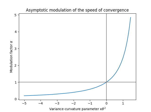
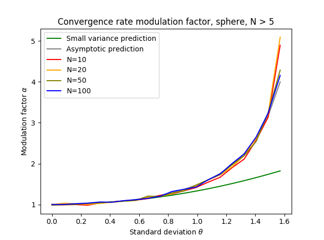
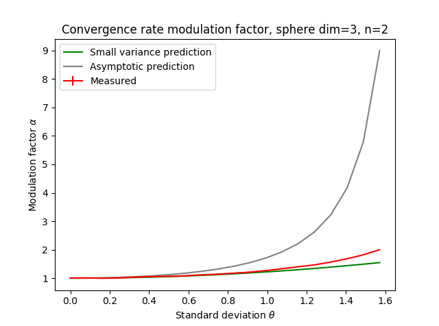
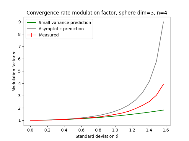
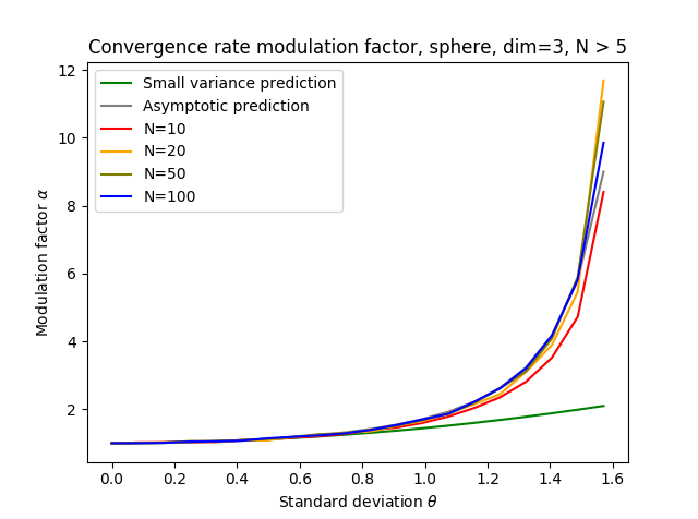
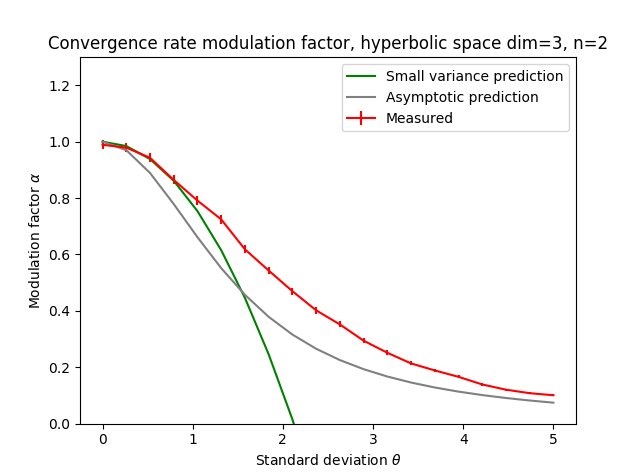
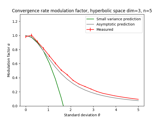
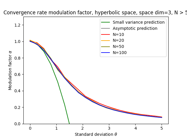
In order to better visualize the influence of the curvature on the empirical mean, we investigate in Section 7 the case of isotropic distributions in constant curvature spaces, also called space forms. In this case, both the asymptotic and the high concentration expansions can be reduced to a scalar equation where the rate of convergence of the variance of the empirical mean with respect to the number of samples is modulated by a scalar factor α=Var(x¯n)n/σ2𝛼Varsubscript¯𝑥𝑛𝑛superscript𝜎2\alpha=\text{Var}(\bar{x}_{n}){n}/{\sigma^{2}} indicating how much the variance of the empirical mean deviates from the Euclidean case: a modulation factor α>1𝛼1\alpha>1 indicates that the convergence is slower than in the Euclidean case, while a value α<1𝛼1\alpha<1 indicates a faster convergence.

The setup can be further simplified by considering a uniform distribution on a Riemannian hypersphere of radius θ𝜃\theta around the population mean x¯¯𝑥\bar{x}. For a large number of samples in a manifold of large dimension, we obtain an archetypal modulation factor α=tan2(κθ2)κθ2𝛼superscript2𝜅superscript𝜃2𝜅superscript𝜃2\alpha=\frac{\tan^{2}(\sqrt{\kappa\theta^{2}})}{\kappa\theta^{2}} on the convergence of the variance of the empirical mean. We see that the variable controlling the modulation is actually κθ2𝜅superscript𝜃2\kappa\theta^{2}, the product of the sectional curvature with the variance. For a positive variance-curvature, the modulation of the rate of convergence is larger than one (the convergence is slower) and goes to infinity when κθ2𝜅superscript𝜃2\kappa\theta^{2} approaches π2/4superscript𝜋24\pi^{2}/4. This corresponds exactly to the Kendall & Karcher concentration conditions under which all the results of this paper are restricted. This was expected since a uniform distributions on a Riemannian hypersphere of radius π/2𝜋2\pi/2 on a sphere fails to have a unique mean: the distribution of the empirical Fréchet mean converges to a mixture of Diracs rather than concentrating on a point as usual. For negative curvature, the modulation factor is below 1, meaning that the convergence is accelerated, and actually goes to zero (an infinite acceleration) for an infinitely negative variance-curvature. Such a phenomenon has been observed in specific cases for other types of means in negatively curves manifolds but was apparently not recognized so far as a general phenomenon of least-squares in manifolds. We conjecture that it is related to the phenomenon of stickiness of the Fréchet mean in stratified spaces.

These theoretical predictions are illustrated by experiments on the 2- and 3-sphere and on the hyperbolic space of dimension 3 which demonstrate that the formulas that we have obtained are very accurate in their own domains.

2 Means on Riemannian and affine connection manifolds

2.1 Riemannian manifolds

We consider a differential manifold {\cal M} provided with a smooth scalar product .|.x\left<\>.\>\left|\>.\right.\right>_{x} on each tangent space Txsubscript𝑇𝑥T_{x}{\cal M} at point x𝑥x of {\cal M}, called the Riemannian metric. In a chart, the metric is fully specified by the dot product of the coordinate vector fields: gij(x)=i|jsubscript𝑔𝑖𝑗𝑥inner-productsubscript𝑖subscript𝑗g_{ij}(x)=\left<\>\partial_{i}\>\left|\>\partial_{j}\right.\right>. The Riemannian distance between any two points on {\cal M} is the infimum of the length of the curves joining these points. Geodesics are defined as the critical points of the energy functional. Geodesics are parametrized by arc-length in addition to optimizing the length functional. We assume in this paper that the manifold is geodesically complete, i.e. that the definition domain of all geodesics can be extended to \mathbb{R}. This means that the manifold has no boundary nor any singular point that we can reach in a finite time. As an important consequence, the Hopf-Rinow-De Rham theorem states that there always exists at least one minimizing geodesic between any two points of the manifold (i.e. whose length is the distance between the two points).

From the theory of second order differential equations, we know that there exists one and only one geodesic γ(x,v)(t)subscript𝛾𝑥𝑣𝑡\gamma_{(x,v)}(t) starting from the point x𝑥x with the tangent vector vTx𝑣subscript𝑇𝑥v\in T_{x}{\cal M} . The exponential map at point x𝑥x maps each tangent vector vTx𝑣subscript𝑇𝑥v\in T_{x}{\cal M} to the point of the manifold that is reached after a unit time by the geodesic: expx(v)=γ(x,v)(1)subscript𝑥𝑣subscript𝛾𝑥𝑣1\exp_{x}(v)=\gamma_{(x,v)}(1). The exponential map is locally one-to-one around 00: we denote by logx(y)subscript𝑥𝑦\log_{x}(y) its inverse. To shorten formulas, we sometimes use the notation xy𝑥𝑦\overrightarrow{xy} instead of logx(y)subscript𝑥𝑦\log_{x}(y).

The cut time tcut(x,v)subscript𝑡𝑐𝑢𝑡𝑥𝑣t_{cut}(x,v) is the maximal time for which the normal geodesic starting at x𝑥x with unit tangent vector vTx𝑣subscript𝑇𝑥v\in T_{x}{\cal M} is length minimizing. By homogeneity, the cut-time can be extended to the tangent bundle T𝑇superscriptT{\cal M}^{*}: tcut(x,v)=tcut(x,v/vx)vxsubscript𝑡𝑐𝑢𝑡𝑥𝑣subscript𝑡𝑐𝑢𝑡𝑥𝑣subscriptnorm𝑣𝑥subscriptnorm𝑣𝑥t_{cut}(x,v)=t_{cut}(x,v/\|v\|_{x})\|v\|_{x}, except for null tangent vectors. The tangent cut-locus is defined as the set of vectors of Tx=Tx{0}subscript𝑇𝑥superscriptsubscript𝑇𝑥0T_{x}{\cal M}^{*}=T_{x}{\cal M}\setminus\{0\} where the distance ceases to be minimizing: C(x)={tcut(x,v)v|vTx}𝐶𝑥conditional-setsubscript𝑡𝑐𝑢𝑡𝑥𝑣𝑣𝑣subscript𝑇𝑥superscriptC(x)=\{t_{cut}(x,v)v|v\in T_{x}{\cal M}^{*}\}. The cut-locus is the image of the tangent cut-locus by the exponential map: Cut(x)=expx(C(x))Cut𝑥subscript𝑥𝐶𝑥\text{Cut}(x)=\exp_{x}(C(x)). The distance to a point x𝑥x is C2superscript𝐶2C^{2} except at the cut locus where it is only continuous. The tangent cut locus delimits a star shaped domain around 00 in each tangent space whose interior is called the injectivity domain of the exponential map:

Inj(x)={tv| 0t<tcut(x,v),vTx}.Inj𝑥conditional-set𝑡𝑣formulae-sequence 0𝑡subscript𝑡𝑐𝑢𝑡𝑥𝑣𝑣subscript𝑇𝑥superscript\text{Inj}(x)=\{tv\>|\>0\leq t<t_{cut}(x,v),v\in T_{x}{\cal M}^{*}\}.

The injection radius is the infimum of the cut values of the various geodesics emanating from x𝑥x (i.e. the radius of the largest open geodesic ball included in the injectivity domain, and thus on which expxsubscript𝑥\exp_{x} is a diffeomorphism):

inj(x)=min{tcut(x,v/vx)|vTx}.inj𝑥conditionalsubscript𝑡𝑐𝑢𝑡𝑥𝑣subscriptnorm𝑣𝑥𝑣subscript𝑇𝑥superscript\text{inj}(x)=\min\{t_{cut}(x,v/\|v\|_{x})\>|\>v\in T_{x}{\cal M}^{*}\}.

There exists multiple notions of convexity in manifolds [4]. We use here the following: an open subset U𝑈U\subset{\cal M} is (strongly) convex if for any points p,qU𝑝𝑞𝑈p,q\in U, there exists a unique minimal geodesic γ𝛾\gamma joining p𝑝p and q𝑞q which belongs entirely to the subset: γU𝛾𝑈\gamma\subset U.

2.2 Convex affine manifolds

An affine manifold is a differential manifold {\cal M} endowed with an affine connection \nabla. Important classes of affine manifolds are: Riemannian manifolds with their Levi-Civita connection, Lie groups with their canonical symmetric space structure, and more generally affine symmetric spaces. The connection allows us to define geodesics as auto-parallel curves, or zero acceleration curves. These geodesics have an affine parametrization that measures relative distances along each geodesic, but there is no reference length to compare relative distances along different geodesics. Convexity may be defined as in Riemannian manifolds: an open set 𝒰𝒰{\cal U}\subset{\cal M} is convex if for every pair of points x,y𝒰𝑥𝑦𝒰x,y\in{\cal U} there exists a unique \nabla-geodesic joining x𝑥x and y𝑦y lying entirely in 𝒰𝒰{\cal U} and that depends smoothly on its endpoints. This allows us to define the logarithm in a unique way within this subset. In that case, (𝒰,)𝒰({\cal U},\nabla) is called a convex (sub)-manifold. Whitehead Theorem tells us that there exists a convex neighborhood at each point of an affine manifold.

2.3 Curvature of a connection

In order to derive Taylor expansions in manifolds, we need to specify the notations for torsion and curvature operators and their coordinates in charts. The torsion tensor T(X,Y)=XYYX[X,Y]=T(Y,X)𝑇𝑋𝑌subscript𝑋𝑌subscript𝑌𝑋𝑋𝑌𝑇𝑌𝑋T(X,Y)=\nabla_{X}Y-\nabla_{Y}X-[X,Y]=-T(Y,X) measures how the skew-symmetric part of the connection differ from the Lie derivative XY=[X,Y]subscript𝑋𝑌𝑋𝑌{\cal L}_{X}Y=[X,Y]. The connection is torsion free if the torsion tensor vanishes identically. Two connections have the same geodesics if they have the same symmetric part (XY+YX)/2subscript𝑋𝑌subscript𝑌𝑋2(\nabla_{X}Y+\nabla_{Y}X)/2. i.e. if they only differ by torsion. Because means and barycenters in manifolds only involve geodesics and not parallel transport, we can restrict our attention to torsion free (also called symmetric) connections. This notably simplifies the expression of the Taylor expansions. In the sequel, all connections are assumed to be symmetric.

The Riemann curvature tensor in affine connection manifolds

The curvature of an affine manifold is described by the (1,3)13(1,3) curvature tensor R:T×T×TTM:𝑅𝑇𝑇𝑇𝑇𝑀R:T{\cal M}\times T{\cal M}\times T{\cal M}\to TM. It is defined from the covariant derivative by evaluation on vector fields u,v,w𝑢𝑣𝑤u,v,w:

R(u,v)w=uvwvuw[u,v]w.𝑅𝑢𝑣𝑤subscript𝑢subscript𝑣𝑤subscript𝑣subscript𝑢𝑤subscript𝑢𝑣𝑤R(u,v)w=\nabla_{u}\nabla_{v}w-\nabla_{v}\nabla_{u}w-\nabla_{[u,v]}w. (1)

The curvature can be interpreted as the difference between parallel transporting the vector w𝑤w along an infinitesimal parallelogram with sides given by u𝑢u and v𝑣v. Two different sign conventions exist for the curvature tensor: the above definition is the one used in a number of reference books in physics and mathematics [31, 30, 34]. Other authors use a minus sign to simplify some of the tensor notations [35, 32, 14, 4]. There exists moreover different conventions for the order of the tensors subscripts. We use here the convention [R(u,v)w]a=Rbcdaucvdwbsuperscriptdelimited-[]𝑅𝑢𝑣𝑤𝑎subscriptsuperscript𝑅𝑎𝑏𝑐𝑑superscript𝑢𝑐superscript𝑣𝑑superscript𝑤𝑏[R(u,v)w]^{a}=R^{a}_{bcd}u^{c}v^{d}w^{b} so that the tensor can be written using the Christoffel symbols ΓbcasubscriptsuperscriptΓ𝑎𝑏𝑐\Gamma^{a}_{bc}:

Rbcda=dxa(R(c,d)b)=cΓdbadΓcba+ΓceaΓdbeΓdeaΓcbe,subscriptsuperscript𝑅𝑎𝑏𝑐𝑑𝑑superscript𝑥𝑎𝑅subscript𝑐subscript𝑑subscript𝑏subscript𝑐subscriptsuperscriptΓ𝑎𝑑𝑏subscript𝑑subscriptsuperscriptΓ𝑎𝑐𝑏subscriptsuperscriptΓ𝑎𝑐𝑒subscriptsuperscriptΓ𝑒𝑑𝑏subscriptsuperscriptΓ𝑎𝑑𝑒subscriptsuperscriptΓ𝑒𝑐𝑏R^{a}_{bcd}=dx^{a}(R(\partial_{c},\partial_{d})\partial_{b})=\partial_{c}\Gamma^{a}_{db}-\partial_{d}\Gamma^{a}_{cb}+\Gamma^{a}_{ce}\Gamma^{e}_{db}-\Gamma^{a}_{de}\Gamma^{e}_{cb}, (2)

where i=/xisubscript𝑖subscript𝑥𝑖\partial_{i}=\partial/\partial x_{i} are coordinate vector fields.

The curvature tensor has several symmetries that we will use to simplify expressions: it is skew-symmetric in the first two variables, and we we have the First and second Bianchi identities.

R(u,v)=R(v,u)𝑅𝑢𝑣𝑅𝑣𝑢\displaystyle R(u,v)=-R(v,u) or Rbcda=Rbdca;subscriptsuperscript𝑅𝑎𝑏𝑐𝑑subscriptsuperscript𝑅𝑎𝑏𝑑𝑐\displaystyle R^{a}_{bcd}=-R^{a}_{bdc};
R(u,v)w+R(v,w)u+R(w,u)v=0𝑅𝑢𝑣𝑤𝑅𝑣𝑤𝑢𝑅𝑤𝑢𝑣0\displaystyle R(u,v)w+R(v,w)u+R(w,u)v=0 or R[bcd]a=Rbcda+Rcdba+Rdbca=0;subscriptsuperscript𝑅𝑎delimited-[]𝑏𝑐𝑑subscriptsuperscript𝑅𝑎𝑏𝑐𝑑subscriptsuperscript𝑅𝑎𝑐𝑑𝑏subscriptsuperscript𝑅𝑎𝑑𝑏𝑐0\displaystyle R^{a}_{[bcd]}=R^{a}_{bcd}+R^{a}_{cdb}+R^{a}_{dbc}=0;
(uR)(v,w)+(vR)(w,u)+(wR)(u,v)=0subscript𝑢𝑅𝑣𝑤subscript𝑣𝑅𝑤𝑢subscript𝑤𝑅𝑢𝑣0\displaystyle(\nabla_{u}R)(v,w)+(\nabla_{v}R)(w,u)+(\nabla_{w}R)(u,v)=0 or Rb[cd;e]a=eRbcda+cRbdea+dRbeca=0.subscriptsuperscript𝑅𝑎𝑏𝑐𝑑𝑒subscript𝑒subscriptsuperscript𝑅𝑎𝑏𝑐𝑑subscript𝑐subscriptsuperscript𝑅𝑎𝑏𝑑𝑒subscript𝑑subscriptsuperscript𝑅𝑎𝑏𝑒𝑐0\displaystyle R^{a}_{b[cd;e]}=\nabla_{e}R^{a}_{bcd}+\nabla_{c}R^{a}_{bde}+\nabla_{d}R^{a}_{bec}=0.

Additional symmetries in a Riemannian manifold

In a Riemannian manifold, we can lower the first coordinate with the metric to obtain the (0,4)04(0,4) version of the Riemannian curvature tensor:

R(u,v,w,z)=R(w,z)v|uor in coordinatesRabcd=gaeRbcde.formulae-sequence𝑅𝑢𝑣𝑤𝑧inner-product𝑅𝑤𝑧𝑣𝑢or in coordinatessubscript𝑅𝑎𝑏𝑐𝑑subscript𝑔𝑎𝑒subscriptsuperscript𝑅𝑒𝑏𝑐𝑑R(u,v,w,z)=\left<\>R(w,z)v\>\left|\>u\right.\right>\quad\text{or in coordinates}\quad R_{abcd}=g_{ae}R^{e}_{bcd}. (3)

This tensor inherits the above symmetries. Additionally, it is symmetric in the first and last two variables, which implies being skew-symmetric in the last two variables:

R(u,v)w|z=R(u,v)z|winner-product𝑅𝑢𝑣𝑤𝑧inner-product𝑅𝑢𝑣𝑧𝑤\displaystyle\left<\>R(u,v)w\>\left|\>z\right.\right>=-\left<\>R(u,v)z\>\left|\>w\right.\right> or Rabcd=Rcdab;subscript𝑅𝑎𝑏𝑐𝑑subscript𝑅𝑐𝑑𝑎𝑏\displaystyle R_{abcd}=R_{cdab};
R(u,v)w|z=R(w,z)u|winner-product𝑅𝑢𝑣𝑤𝑧inner-product𝑅𝑤𝑧𝑢𝑤\displaystyle\left<\>R(u,v)w\>\left|\>z\right.\right>=\left<\>R(w,z)u\>\left|\>w\right.\right> or Rabcd=Rabdc.subscript𝑅𝑎𝑏𝑐𝑑subscript𝑅𝑎𝑏𝑑𝑐\displaystyle R_{abcd}=-R_{abdc}.

This means in particular that its contraction with any symmetric tensor in the first two or last two indices is zero.

Note that in an affine manifold with an auxiliary metric g𝑔g we can also lower the first index of the curvature tensor, but this metric should be kept in all computations as it is not the identity in a normal coordinate system and its covariant derivative is not zero as with the Levi-Civita connection.

Sectional curvature

In Riemannian manifolds, the sectional curvature κ(u,v)(x)𝜅𝑢𝑣𝑥\kappa(u,v)(x) measures the Gaussian curvature (the product of the principal curvatures) in the 2-planes of Txsubscript𝑇𝑥T_{x}{\cal M} generated by the vectors u𝑢u and v𝑣v. It can be expressed from the curvature tensor by:

κ(u,v)(x)=R(u,v)v|uxux2vx2u|vx2.𝜅𝑢𝑣𝑥subscriptinner-product𝑅𝑢𝑣𝑣𝑢𝑥superscriptsubscriptnorm𝑢𝑥2superscriptsubscriptnorm𝑣𝑥2superscriptsubscriptinner-product𝑢𝑣𝑥2\kappa(u,v)(x)=\frac{\left<\>R(u,v)v\>\left|\>u\right.\right>_{x}}{\|u\|_{x}^{2}\|v\|_{x}^{2}-\left<\>u\>\left|\>v\right.\right>_{x}^{2}}\,. (4)

The upper bound of the sectional curvature plays a very important role for convexity in Riemannian manifolds, as we will see below.

2.4 Moments of a probability measure

Definition 1

Let μProb()𝜇𝑃𝑟𝑜𝑏\mu\in{Prob}({\cal M}) be a probability measure on a manifold {\cal M}. The k𝑘k-order moment of μ𝜇\mu is the (k,0)𝑘0(k,0) tensor:

𝔐kμ(x)=logx(y)logx(y)logx(y)k timesμ(dy)=logx(y)kμ(dy){\mathfrak{M}}_{k}\mu(x)=\int_{\cal M}\underbrace{\log_{x}(y)\otimes\log_{x}(y)\ldots\otimes\log_{x}(y)}_{\text{$k$ times}}\>\mu(dy)=\int_{\cal M}\log_{x}(y)^{\otimes k}\>\mu(dy) (5)

For a general distribution in a Riemannian manifold, the tensor field is not defined (and non-smooth) at points where the cut locus has a non-zero mass. If the density μ𝜇\mu is uniformly bounded by the Riemannian measure (i.e. if μ(dx)=μ(x)d(x)𝜇𝑑𝑥𝜇𝑥𝑑𝑥\mu(dx)=\mu(x)d{\cal M}(x)), then this integral defines a smooth (k,0)𝑘0(k,0) tensor field over {\cal M} since the cut locus of the point x𝑥x has null measure. In an affine manifold, the support of μ𝜇\mu needs to be limited to an convex neighborhood so that the logarithm is well defined and all moments are smooth within this neighborhood. The 0-th order moment 𝔐0μ=𝑑μ(x)=1subscript𝔐0𝜇subscriptdifferential-d𝜇𝑥1{\mathfrak{M}}_{0}\mu=\int_{{\cal M}}d\mu(x)=1 is unit by definition. The first order moment 𝔐1μ(x)=xxi𝑑μ(x)subscript𝔐1𝜇𝑥subscript𝑥subscript𝑥𝑖differential-d𝜇𝑥{\mathfrak{M}}_{1}\mu(x)=\int_{{\cal M}}\overrightarrow{xx_{i}}\>d\mu(x) is a vector field on the manifold {\cal M}.

In the following, we only consider distributions that have support in a convex affine manifold (,)({\cal M},\nabla) that is fixed once for all. Such a convex manifold is diffeomorphic to an open set of dsuperscript𝑑\mathbb{R}^{d}. Cartan-Hadamard manifolds (complete, simply connected manifolds with sectional curvature less than or equal to 0) are classical convex complete Riemannian manifolds. Examples of incomplete convex manifolds are given by small geodesic balls in Riemannian manifolds or small balls centered at the origin in an exponential chart in an affine manifold [2].

2.5 Means on Riemannian manifolds

The classical mean value of random numeric values with distribution μ𝜇\mu is defined through an integral x¯=xμ(dx)¯𝑥𝑥𝜇𝑑𝑥\bar{x}=\int x\>\mu(dx). Because μ𝜇\mu is normalized, this definition can be rewritten as an implicit barycentric equation: (xx¯)μ(dx)𝑥¯𝑥𝜇𝑑𝑥\int(x-\bar{x})\>\mu(dx). With this formulation, it is obvious that this notion is affine and not metric. In the context of probability and statistics, Maurice Fréchet was the first to unify several type of typical statistical values, in particular the mean and the median, and to generalize them to abstract spaces. In a preparatory work, he first investigated [17] different ways to compute mean values of random triangles, independently of their position and orientation in space, with experiments to confront the theoretical results to real world data. In this respect, he may be considered as pioneering the statistical study of shapes. In a second study, motivated by the study of random curves, he first introduced a mean value and a law of large numbers defined by a generalization of the integral to normed vector (Wiener or Banach) space. Finally, Fréchet considered in [18, p.233] a family of central values (including the mean and the median) and its generalization to random elements in abstract metric spaces:

Definition 2 (Fréchet mean in a metric space [18])

The p𝑝p-mean (typical position of order p𝑝p according to Fréchet) of a distribution (a random element) μ𝜇\mu in an abstract metric space {\cal M} is set of minima of the p𝑝p-standard deviation :

p-Mean(μ)={argminydist(x,y)pμ(dx)}.p-Mean𝜇𝑦subscriptdistsuperscript𝑥𝑦𝑝𝜇𝑑𝑥\textstyle\text{p-Mean}(\mu)=\left\{\underset{y\in{\cal M}}{\arg\min}\;\int_{\cal M}\>\mbox{\rm dist}(x,y)^{p}\>\mu(dx)\right\}. (6)

The case p=2𝑝2p=2 corresponds in vector spaces to the arithmetic mean, the case p=1𝑝1p=1 to the median (“equiprobable value” in Fréchet’s words).

The first key contribution of Fréchet was to consider many different types of typical elements, including of course the mean but also the median. Fréchet considered mainly the case p1𝑝1p\geq 1, but he observed that many of the properties could be also generalized to 0<p<10𝑝10<p<1. His second revolutionary idea was to considered a set of mean elements rather than one unique mean. This idea was later developed by Ziezold [37] with a strong law of large numbers for sets of random elements in separable finite quasi-metric spaces. These two innovations justify the name of Fréchet mean that is used in geometric statistics.

For smooth differential geometric spaces like Riemannian manifolds, and restricting to the classical 2-mean, Berger [4, p.235] reported that “the existence of a unique center of mass in the large for manifolds with non-positive curvature was proven and used by Élie Cartan back in the 1920’s.” In order to find the fixed point of a group of isometries, Cartan indeed showed in [11] that the sum of the square distances from one point to a finite number of points has a unique minimum in simply connected Riemannian manifolds with non-positive curvature333Note III on normal spaces with negative or null Riemannian curvature, p. 267. (now called a Hadamard space). This result was extended in [12] to closed subgroups of isometries. It is obvious in this text that Cartan is only using the uniqueness of the minimum of the sum of square distances as a tool in the specific case of negative curvature Riemannian manifolds and not as a general definition of the mean on manifolds as usually thought in probability or statistics.

For similar purposes, Grove and Karcher extended this idea in 1973 to positive curvature manifolds for distributions with sufficiently small support, typically within convex balls so that the mean exists and is unique [21]. The notion was coined the Riemannian center of mass. In this publication and in successive ones, Karcher and colleagues determined Jacobi field estimates to find optimal conditions for the convexity of the ball that support this definition. The Riemannian barycenter is commonly refered to as describes in [24] but the most complete description of the related properties is certainly found in [9], where a notion of barycenter in affine connection manifolds is also worked out. A good historical note on the history of the Riemannian barycenter is given in [1] and by Karcher himself in [25].

In all these works, the Riemannian center of mass is unique by definition. Considering a set-valued barycenter on an affine connection manifold was the contribution of Emery and Mokobodzki:

Definition 3 (Exponential barycenters in an affine connection manifold [16])

We consider a probability measure μ𝜇\mu with support in a convex local neighborhood 𝒰𝒰{\cal U} of an affine connection manifold (,)({\cal M},\nabla). Exponential barycenters of the probability measure μ𝜇\mu are the points

Bary𝒰(μ)={x𝒰|𝔐1(x)=logx(y)μ(dy)=0}.subscriptBary𝒰𝜇conditional-set𝑥𝒰subscript𝔐1𝑥subscriptsubscript𝑥𝑦𝜇𝑑𝑦0\text{Bary}_{{\cal U}}(\mu)=\left\{x\in{\cal U}\>|\>{\mathfrak{M}}_{1}(x)=\int_{{\cal M}}\log_{x}(y)\>\mu(dy)=0\right\}.

The non-uniqueness of the expectation of a random variable considerably extended the usability of this definition, in particular in positive curvature manifolds. We notice that the notion remains purely affine, provided that the distribution has a support on a convex neighborhood in which the logarithm can be defined uniquely. In the Riemannian case, [16] showed that exponential barycenters are the critical points of the variance. Thus exponential barycenters contain in particular the minimum of the variance σ2(x)=dist2(x,y)μ(dy)superscript𝜎2𝑥subscriptsuperscriptdist2𝑥𝑦𝜇𝑑𝑦\sigma^{2}(x)=\int_{\cal M}\>\mbox{\rm dist}^{2}(x,y)\>\mu(dy) (sometimes called the Fréchet functional), except if the variance is not differentiable at this point.

The optimal conditions for the existence and uniqueness of the minimum of the variance have been studied in [24, 9, 27, 28, 29]. The result has been extended to Fréchet p𝑝p-means defined as the minima of the p𝑝p-variance in [1, 36]. The Hessian of the squared distance to a point plays a key role in these conditions. Karcher looked for a ball where this Hessian is positive definite everywhere, while Kendall relaxed this condition to the locus of the minimum. We will see in Section 7.3 that the inverse of the expected Hessian also controls the speed of convergence to the mean, so that the non-uniqueness may also be interpreted as an absence of convergence.

Theorem 1 (Karcher & Kendall Concentration (KKC) Conditions)

Let {\cal M} be a geodesically complete Riemannian manifold with injection radius inj(x)inj𝑥\text{inj}(x) Let μ𝜇\mu is a probability distribution on {\cal M} whose support is contained in a closed regular geodesic ball B¯(x,r)¯𝐵𝑥𝑟\bar{B}(x,r) of radius r<12inj(x)𝑟12inj𝑥r<\frac{1}{2}\text{inj}(x). We assume moreover that the upper bound κ=supyB(x,r),uvTyκ(u,v)(y)𝜅subscriptsupremumformulae-sequence𝑦𝐵𝑥𝑟𝑢𝑣subscript𝑇𝑦𝜅𝑢𝑣𝑦\kappa=\sup_{y\in B(x,r),u\not=v\in T_{y}{\cal M}}\kappa(u,v)(y) of the sectional curvatures in the ball satisfies κ<π2/(2r)2𝜅superscript𝜋2superscript2𝑟2\kappa<\pi^{2}/(2r)^{2}. This second condition is always verified on spaces of negative curvature and it specifies a maximal radius r=π2κsuperscript𝑟𝜋2𝜅r^{*}=\frac{\pi}{2\sqrt{\kappa}} when there is positive sectional curvature. These concentration assumptions ensure that the variance has a unique global minimum that belongs to the ball B¯(x,r)¯𝐵𝑥𝑟\bar{B}(x,r).

In order to differentiate the different notions of means in Riemannian manifolds, it is usual in geometric statistics to name Fréchet mean the set of global minima of the variance, Karcher mean the set of local minima, and exponential barycenters the set of critical points satisfying the implicit equation 𝔐1(x)=0subscript𝔐1𝑥0{\mathfrak{M}}_{1}(x)=0. It is clear that all these definition boil down to the same unique point within the ball B(x,r)𝐵𝑥𝑟B(x,r) in KKC conditions for the classical 2-mean, although some local minima and critical points may exist outside this ball. Throughout this paper, we assume that the support of all the distributions that we consider on Riemannian manifolds are included in a regular geodesic ball B(x0,r)𝐵subscript𝑥0𝑟B(x_{0},r) of diameter 2r<ε2𝑟𝜀2r<\varepsilon that satisfies the KKC conditions. As a consequence, one can conclude that there is a unique exponential barycenter x¯¯𝑥\bar{x} included in the ball, necessarily the Fréchet mean [24, 27]. The maximal diameter ε𝜀\varepsilon of the support of the distribution is used in this paper as the scale variable to control Taylor expansions.

2.6 Means in convex affine connection manifolds

To define the mean of a probability distribution μ𝜇\mu in a convex manifold (,)({\cal M},\nabla), we cannot rely on the Fréchet mean since there is no distance. However, the notion of exponential barycenter still makes sense because the affine logarithm is well defined [16]: they are the zeros of the first moment field 𝔐1(μ)=logx(y)μ(dy)subscript𝔐1𝜇subscriptsubscript𝑥𝑦𝜇𝑑𝑦{\mathfrak{M}}_{1}(\mu)=\int_{{\cal M}}\log_{x}(y)\>\mu(dy) for xM𝑥𝑀x\in M. This definition, studied in [9, 16], is close to the Riemannian center of mass but uses the logarithm of the affine connection in a convex domain instead of the Riemannian logarithm in the injectivity domain.

Distributions with compact support in a convex affine manifold have at least one exponential barycenter. Moreover, exponential barycenter are stable by affine diffeomorphisms (connection preserving maps, which thus preserve the geodesics and the normal convex neighborhoods) [9]. However, the classical notion of convexity is not sufficient to ensure the uniqueness of the mean. For that purpose, stronger convexity conditions have been proposed.

Definition 4 (Arnaudon & Li convexity (ALC) conditions [2])

Let (,)({\cal M},\nabla) be an affine manifold. A separating function on {\cal M} is a convex function ρ:×+:𝜌superscript\rho:{\cal M}\times{\cal M}\rightarrow\mathbb{R}^{+} vanishing exactly on the diagonal of the product manifold (considered as an affine manifold with the direct product connection). Here, convex means that the restriction of ρ(γ(t))𝜌𝛾𝑡\rho(\gamma(t)) to any geodesic γ(t)𝛾𝑡\gamma(t) of ×{\cal M}\times{\cal M} is a convex function from \mathbb{R} to +superscript\mathbb{R}^{+}. A manifold which carries a smooth separating function ρ𝜌\rho such that

cdist(x,y)pρ(x,y)Cdist(x,y)p,𝑐distsuperscript𝑥𝑦𝑝𝜌𝑥𝑦𝐶distsuperscript𝑥𝑦𝑝c\>\>\mbox{\rm dist}(x,y)^{p}\leq\rho(x,y)\leq C\>\>\mbox{\rm dist}(x,y)^{p},

for some constants 0<c<C0𝑐𝐶0<c<C, some positive integer p2𝑝2p\geq 2 and some auxiliary Riemannian distance function  dist is called a manifold with p𝑝p-convex geometry. On a manifold with p𝑝p-convex geometry, every compactly supported probability measure has a unique exponential barycenter.

Whitehead theorem tells us in essence that any point in an affine connection manifold has a convex neighborhood with 2-convex geometry. In Riemannian manifolds, geodesic balls in KKC conditions have 2-convex geometry. These conditions will be sufficient for our goal of studying the behavior of the empirical means with high concentration. We should note that the notion is too strong in general since there are examples of manifolds where one can prove uniqueness although they do not have p𝑝p-convex geometry for any p𝑝p. This has motivated the definition of CSLCG (convex, with semi-local convex geometry) manifolds in [2] but we will not need it in this paper.

Throughout this paper, we only consider distributions that satisfy the ALC condition, i.e. compact distributions in a convex affine manifold (,)({\cal M},\nabla) with p𝑝p-convex geometry. With this extra structure, we have an auxiliary Riemannian metric on {\cal M} whose norm in Txsubscript𝑇𝑥T_{x}{\cal M} is denoted .x\|.\|_{x} and whose Riemannian distance is denoted  dist. Thanks to this distance, we can compute the diameter ε𝜀\varepsilon of the support of the distribution, which is then used as in Riemannian manifolds as the typical scale variable to control Taylor expansions.

3 Taylor expansions in Riemannian and affine manifolds

In order to analyze the variance of a random element in a Riemannian manifold, we may compute the Taylor expansion of the squared Riemannian distance functions in a local coordinate system. This requires to have an expression for the geodesics. In a normal coordinate system centered at x𝑥x, a geodesic starting at x𝑥x with tangent vector v𝑣v is a straight line: logx(expx(tv))=tvsubscript𝑥subscript𝑥𝑡𝑣𝑡𝑣\log_{x}(\exp_{x}(tv))=tv. However, the geodesic starting at xv=expx(v)subscript𝑥𝑣subscript𝑥𝑣x_{v}=\exp_{x}(v) and ending at xw=expx(w)subscript𝑥𝑤subscript𝑥𝑤x_{w}=\exp_{x}(w) deviates from the straight line from v𝑣v to w𝑤w in our chart because of curvature. Geodesic may be approximated by a polynomial expansion in the variables v𝑣v and w𝑤w that solves the geodesic equation.

The expansion of the Riemannian logarithm can be based on the Taylor expansion of the Riemannian metric in a normal coordinate system. Such an extension is well known for the first orders, but going to orders higher than 4 is computationally much more involved and requires computational algebraic methods such as the ones developed by Brewin [8]. Part of the results presented in this paper were originally developed in 2015 using this method. However, the intelligibility of the formulas involving lots of terms and indices was difficult.

In this paper, we base our Taylor expansions on a more geometric formulation based on a coordinate free expansion of the composition of two exponential maps developed by Gavrilov [19, 20]. This formula only involves the curvature and torsion tensors and their covariant derivatives at the development point. Moreover, the proposed extension relies only on the connection and not on the Riemannian metric, which makes it immediately suitable for the general affine connection case.

3.1 Gavrilov’s expansions of the double exponential in affine manifolds

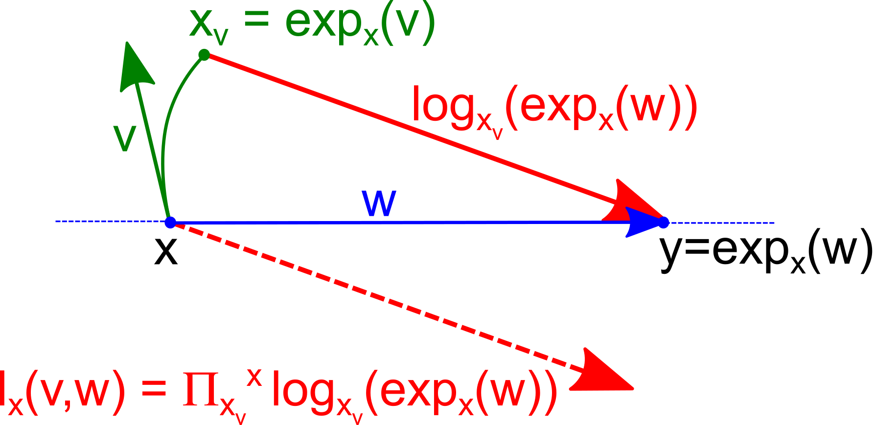
In the spirit of the Baker-Campbell-Hausdorff (BCH) formula for Lie groups, Gavrilov [19, 20] developed a coordinate free expansion of the composition of two exponential maps. The double exponential expx(v,u)=expexpx(v)(Πxexpx(v)u)subscript𝑥𝑣𝑢subscriptsubscript𝑥𝑣superscriptsubscriptΠ𝑥subscript𝑥𝑣𝑢\exp_{x}(v,u)=\exp_{\exp_{x}(v)}(\Pi_{x}^{\exp_{x}(v)}u) corresponds to a first geodesic shooting from the point x𝑥x along the vector v𝑣v, followed by a second geodesic shooting from y=expx(v)𝑦subscript𝑥𝑣y=\exp_{x}(v) along the parallel transport ΠxyusuperscriptsubscriptΠ𝑥𝑦𝑢\Pi_{x}^{y}u of the vector u𝑢u along the first geodesic (Fig. 1, left). This expansion holds in general affine connection manifolds, and has a surprisingly simple coordinate free formulation. We formulate it here in the torsion free case.

Theorem 2 (The double exponential expansion [19, 20])

In a torsion-free affine connection manifold, the log of the double exponential hx(v,u)=logx(expx(v,u))subscript𝑥𝑣𝑢subscript𝑥subscript𝑥𝑣𝑢h_{x}(v,u)=\log_{x}(\exp_{x}(v,u)) has the following series expansion in v𝑣v and w𝑤w at order 5:

hx(v,u)=v+u+16R(u,v)v+13R(u,v)u+124(vR)(u,v)(2v+5u)+124(uR)(u,v)(v+2u)+O(5),subscript𝑥𝑣𝑢𝑣𝑢16𝑅𝑢𝑣𝑣13𝑅𝑢𝑣𝑢124subscript𝑣𝑅𝑢𝑣2𝑣5𝑢124subscript𝑢𝑅𝑢𝑣𝑣2𝑢𝑂5\begin{split}h_{x}(v,u)=\,&v+u+\frac{1}{6}R(u,v)v+\frac{1}{3}R(u,v)u+\frac{1}{24}(\nabla_{v}R)(u,v)(2v+5u)\\ &+\frac{1}{24}(\nabla_{u}R)(u,v)(v+2u)+O(5),\end{split} (7)

where O(5)𝑂5O(5) represents polynomial terms of order 5 or more in u and v.

In the right-hand side, the tensor values are taken at x𝑥x. By extending the vectors u𝑢u and v𝑣v of Txsubscript𝑇𝑥T_{x}{\cal M} to vector fields in the neighborhood of x𝑥x using parallel transport, we see that the series is valid point-wise at any point in that neighborhood.

The fundamental idea of this expansion is the use of parallel transport to identify tangent spaces rather than the differential of the exponential as is implicitly done in Taylor expansions in normal coordinate systems [8]. This trick drastically simplifies the expressions with coordinate free expressions. We notice that hxsubscript𝑥h_{x} is a mapping of vector spaces from Tx×Txsubscript𝑇𝑥subscript𝑇𝑥T_{x}{\cal M}\times T_{x}{\cal M} to Txsubscript𝑇𝑥T_{x}{\cal M}.

Refer to caption
Refer to caption
Figure 1: Left: the log of the composition of two exponentials (BCH-type formula) in a normal coordinate system at x. Right: The neighboring log of a fixed point expx(w)subscript𝑥𝑤\exp_{x}(w) when the foot-point x𝑥x is moved along the geodesic xv=expx(v)subscript𝑥𝑣subscript𝑥𝑣x_{v}=\exp_{x}(v), in a normal coordinate system at x.

3.2 Moving the foot-point: the neighboring log expansion

The double exponential formula may be used to evaluate how the log of a fixed point y=expx(w)𝑦subscript𝑥𝑤y=\exp_{x}(w) is modified when x𝑥x is moved along the geodesic xv=expx(v)subscript𝑥𝑣subscript𝑥𝑣x_{v}=\exp_{x}(v): we define the neighboring log as lx(v,w)=Πxvxlogxv(expx(w))subscript𝑙𝑥𝑣𝑤superscriptsubscriptΠsubscript𝑥𝑣𝑥subscriptsubscript𝑥𝑣subscript𝑥𝑤l_{x}(v,w)=\Pi_{x_{v}}^{x}\log_{x_{v}}(\exp_{x}(w)) (Fig. 1, right). This amounts to say that the vector u=lx(v,w)𝑢subscript𝑙𝑥𝑣𝑤u=l_{x}(v,w) is solution of expxv(Πxxvu)=expx(w)subscriptsubscript𝑥𝑣superscriptsubscriptΠ𝑥subscript𝑥𝑣𝑢subscript𝑥𝑤\exp_{x_{v}}(\Pi_{x}^{x_{v}}u)=\exp_{x}(w). We recognize the double exponential expx(v,u)subscript𝑥𝑣𝑢\exp_{x}(v,u) on the left-hand side. Thus, determining u=lx(v,w)𝑢subscript𝑙𝑥𝑣𝑤u=l_{x}(v,w) amounts to solve hx(v,u)=logx(expx(v,u))=wsubscript𝑥𝑣𝑢subscript𝑥subscript𝑥𝑣𝑢𝑤h_{x}(v,u)=\log_{x}(\exp_{x}(v,u))=w.

The first order solution of hx(v,u)=wsubscript𝑥𝑣𝑢𝑤h_{x}(v,u)=w is obviously u=wv+O(2)𝑢𝑤𝑣𝑂2u=w-v+O(2). To find the second order, we assume that u=wv+u2+O(3)𝑢𝑤𝑣subscript𝑢2𝑂3u=w-v+u_{2}+O(3) where u2subscript𝑢2u_{2} is an unknown polynomial expression of order 2 in v𝑣v and w𝑤w. Plugging this value in Eq.7 gives u2=O(3)subscript𝑢2𝑂3u_{2}=O(3) since the curvature terms are of order 3. Assuming a third order term u3subscript𝑢3u_{3}, we now get:

hx(v,wv+u3+O(4))=w+u316R(w,v)v+13R(w,v)w+O(4).subscript𝑥𝑣𝑤𝑣subscript𝑢3𝑂4𝑤subscript𝑢316𝑅𝑤𝑣𝑣13𝑅𝑤𝑣𝑤𝑂4h_{x}(v,w-v+u_{3}+O(4))=w+u_{3}-\frac{1}{6}R(w,v)v+\frac{1}{3}R(w,v)w+O(4).

Thus we find u3=16R(w,v)(v2w)subscript𝑢316𝑅𝑤𝑣𝑣2𝑤u_{3}=\frac{1}{6}R(w,v)(v-2w). Finally, assuming a forth-order term u4subscript𝑢4u_{4} in u=wv+16R(w,v)(v2w)+u4+O(5)𝑢𝑤𝑣16𝑅𝑤𝑣𝑣2𝑤subscript𝑢4𝑂5u=w-v+\frac{1}{6}R(w,v)(v-2w)+u_{4}+O(5) gives:

hx(v,u)=w+u4+124(vR)(w,v)(5w3v)+124((wv)R)(w,v)(2wv)+O(5),subscript𝑥𝑣𝑢𝑤subscript𝑢4124subscript𝑣𝑅𝑤𝑣5𝑤3𝑣124subscript𝑤𝑣𝑅𝑤𝑣2𝑤𝑣𝑂5\begin{split}h_{x}(v,u)=w+u_{4}+\frac{1}{24}(\nabla_{v}R)(w,v)(5w-3v)+\frac{1}{24}(\nabla_{(w-v)}R)(w,v)(2w-v)+O(5),\end{split}

so that hx(v,u)=wsubscript𝑥𝑣𝑢𝑤h_{x}(v,u)=w implies u4=124(vR)(w,v)(2v3w)+124(wR)(w,v)(v2w)subscript𝑢4124subscript𝑣𝑅𝑤𝑣2𝑣3𝑤124subscript𝑤𝑅𝑤𝑣𝑣2𝑤u_{4}=\frac{1}{24}(\nabla_{v}R)(w,v)(2v-3w)+\frac{1}{24}(\nabla_{w}R)(w,v)(v-2w).

Theorem 3 (The neighboring log expansion)

In a torsion-free affine connection manifold, the neighboring log lx(v,w)=Πxvxlogxv(expx(w))subscript𝑙𝑥𝑣𝑤superscriptsubscriptΠsubscript𝑥𝑣𝑥subscriptsubscript𝑥𝑣subscript𝑥𝑤l_{x}(v,w)=\Pi_{x_{v}}^{x}\log_{x_{v}}(\exp_{x}(w)) has the following series expansion in v𝑣v and w𝑤w at order 5:

lx(v,w)=wv+16R(w,v)(v2w)+124(vR)(w,v)(2v3w)+124(wR)(w,v)(v2w)+O(5).subscript𝑙𝑥𝑣𝑤𝑤𝑣16𝑅𝑤𝑣𝑣2𝑤124subscript𝑣𝑅𝑤𝑣2𝑣3𝑤124subscript𝑤𝑅𝑤𝑣𝑣2𝑤𝑂5\begin{split}l_{x}(v,w)=&w-v+\frac{1}{6}R(w,v)(v-2w)\\ &+\frac{1}{24}(\nabla_{v}R)(w,v)(2v-3w)+\frac{1}{24}(\nabla_{w}R)(w,v)(v-2w)+O(5).\end{split} (8)

3.3 Expansion of the Riemannian distance

With the neighboring log expansion, we can now come back to the expansion of the squared Riemannian distance between two points xv=expx(v)subscript𝑥𝑣subscript𝑥𝑣x_{v}=\exp_{x}(v) and xw=expx(w)subscript𝑥𝑤subscript𝑥𝑤x_{w}=\exp_{x}(w) that are close to x𝑥x:

dist(xv,xw)2=logxv(xw)xv2=Πxvxlogxv(xw)x2=lx(v,w)x2=wvx2+13R(w,v)(v2w)|wvx+112(vR)(w,v)(2v3w)|wvx+112(wR)(w,v)(v2w)|wvx+O(6).distsuperscriptsubscript𝑥𝑣subscript𝑥𝑤2subscriptsuperscriptdelimited-∥∥subscriptsubscript𝑥𝑣subscript𝑥𝑤2subscript𝑥𝑣subscriptsuperscriptdelimited-∥∥superscriptsubscriptΠsubscript𝑥𝑣𝑥subscriptsubscript𝑥𝑣subscript𝑥𝑤2𝑥superscriptsubscriptdelimited-∥∥subscript𝑙𝑥𝑣𝑤𝑥2subscriptsuperscriptdelimited-∥∥𝑤𝑣2𝑥13subscriptinner-product𝑅𝑤𝑣𝑣2𝑤𝑤𝑣𝑥112subscriptinner-productsubscript𝑣𝑅𝑤𝑣2𝑣3𝑤𝑤𝑣𝑥112subscriptinner-productsubscript𝑤𝑅𝑤𝑣𝑣2𝑤𝑤𝑣𝑥𝑂6\begin{split}\>\mbox{\rm dist}(x_{v},x_{w})^{2}&=\|\log_{x_{v}}(x_{w})\|^{2}_{x_{v}}=\|\Pi_{x_{v}}^{x}\log_{x_{v}}(x_{w})\|^{2}_{x}=\|l_{x}(v,w)\|_{x}^{2}\\ &=\|w-v\|^{2}_{x}+\frac{1}{3}\left<\>R(w,v)(v-2w)\>\left|\>w-v\right.\right>_{x}\\ &\quad+\frac{1}{12}\left<\>(\nabla_{v}R)(w,v)(2v-3w)\>\left|\>w-v\right.\right>_{x}\\ &\quad+\frac{1}{12}\left<\>(\nabla_{w}R)(w,v)(v-2w)\>\left|\>w-v\right.\right>_{x}+O(6).\end{split}

We now exploit the skew symmetry R(u,v)w|z=R(u,v)z|winner-product𝑅𝑢𝑣𝑤𝑧inner-product𝑅𝑢𝑣𝑧𝑤\left<\>R(u,v)w\>\left|\>z\right.\right>=-\left<\>R(u,v)z\>\left|\>w\right.\right> to simplify the terms of order 4: R(w,v)(v2w)|wv=R(w,v)v|w+2R(w,v)w|v=R(w,v)w|v.inner-product𝑅𝑤𝑣𝑣2𝑤𝑤𝑣inner-product𝑅𝑤𝑣𝑣𝑤2inner-product𝑅𝑤𝑣𝑤𝑣inner-product𝑅𝑤𝑣𝑤𝑣\left<\>R(w,v)(v-2w)\>\left|\>w-v\right.\right>=\left<\>R(w,v)v\>\left|\>w\right.\right>+2\left<\>R(w,v)w\>\left|\>v\right.\right>=\left<\>R(w,v)w\>\left|\>v\right.\right>. The derived skew-symmetry for the covariant derivative (vR)(w,v)u|z=(vR)(w,v)z|uinner-productsubscript𝑣𝑅𝑤𝑣𝑢𝑧inner-productsubscript𝑣𝑅𝑤𝑣𝑧𝑢\left<\>(\nabla_{v}R)(w,v)u\>\left|\>z\right.\right>=-\left<\>(\nabla_{v}R)(w,v)z\>\left|\>u\right.\right> allows us to simplify the terms of order 5:

(vR)(w,v)(2v3w)|wvx=2vR(w,v)v|wx+3vR(w,v)w|vx=vR(w,v)w|vx.subscriptinner-productsubscript𝑣𝑅𝑤𝑣2𝑣3𝑤𝑤𝑣𝑥2subscriptinner-productsubscript𝑣𝑅𝑤𝑣𝑣𝑤𝑥3subscriptinner-productsubscript𝑣𝑅𝑤𝑣𝑤𝑣𝑥subscriptinner-productsubscript𝑣𝑅𝑤𝑣𝑤𝑣𝑥\textstyle\left<\>(\nabla_{v}R)(w,v)(2v-3w)\>\left|\>w-v\right.\right>_{x}=2\left<\>\nabla_{v}R(w,v)v\>\left|\>w\right.\right>_{x}+3\left<\>\nabla_{v}R(w,v)w\>\left|\>v\right.\right>_{x}=\left<\>\nabla_{v}R(w,v)w\>\left|\>v\right.\right>_{x}.
(wR)(w,v)(v2w)|wvx=wR(w,v)v|wx+2wR(w,v)w|vx=wR(w,v)w|vx.subscriptinner-productsubscript𝑤𝑅𝑤𝑣𝑣2𝑤𝑤𝑣𝑥subscriptinner-productsubscript𝑤𝑅𝑤𝑣𝑣𝑤𝑥2subscriptinner-productsubscript𝑤𝑅𝑤𝑣𝑤𝑣𝑥subscriptinner-productsubscript𝑤𝑅𝑤𝑣𝑤𝑣𝑥\textstyle\left<\>(\nabla_{w}R)(w,v)(v-2w)\>\left|\>w-v\right.\right>_{x}=\left<\>\nabla_{w}R(w,v)v\>\left|\>w\right.\right>_{x}+2\left<\>\nabla_{w}R(w,v)w\>\left|\>v\right.\right>_{x}=\left<\>\nabla_{w}R(w,v)w\>\left|\>v\right.\right>_{x}.

Finally, we obtain the Taylor expansion of the squared geodesic distance in a Riemannian manifold between two points xv=expx(v)subscript𝑥𝑣subscript𝑥𝑣x_{v}=\exp_{x}(v) and xw=expx(w)subscript𝑥𝑤subscript𝑥𝑤x_{w}=\exp_{x}(w) that are close to x𝑥x:

dist2(xv,xw)=wvx2+13R(w,v)w,vx+112(v+w)R(w,v)w,vx+O(6).superscriptdist2subscript𝑥𝑣subscript𝑥𝑤subscriptsuperscriptdelimited-∥∥𝑤𝑣2𝑥13subscript𝑅𝑤𝑣𝑤𝑣𝑥112subscriptsubscript𝑣𝑤𝑅𝑤𝑣𝑤𝑣𝑥𝑂6\begin{split}\>\mbox{\rm dist}^{2}(x_{v},x_{w})=\,&\|w-v\|^{2}_{x}+\frac{1}{3}\left<R(w,v)w\,,\,v\right>_{x}+\frac{1}{12}\left<\nabla_{(v+w)}R(w,v)w\,,\,v\right>_{x}+O(6).\end{split} (9)

In coordinates, using the orthonormal property of a normal coordinate system, this reads: dist2(xv,xw)=(wv)a(wv)a+13Rabcdvawbwcvd+112eRabcdvawbwcvd(w+v)e+O(6)superscriptdist2subscript𝑥𝑣subscript𝑥𝑤superscript𝑤𝑣𝑎subscript𝑤𝑣𝑎13subscript𝑅𝑎𝑏𝑐𝑑superscript𝑣𝑎superscript𝑤𝑏superscript𝑤𝑐superscript𝑣𝑑112subscript𝑒subscript𝑅𝑎𝑏𝑐𝑑superscript𝑣𝑎superscript𝑤𝑏superscript𝑤𝑐superscript𝑣𝑑superscript𝑤𝑣𝑒𝑂6\>\mbox{\rm dist}^{2}(x_{v},x_{w})=(w-v)^{a}(w-v)_{a}+\frac{1}{3}R_{abcd}v^{a}w^{b}w^{c}v^{d}+\frac{1}{12}\nabla_{e}R_{abcd}v^{a}w^{b}w^{c}v^{d}(w+v)^{e}+O(6).

4 Expansion of the first moment of the mean

Let μ𝜇\mu be a probability distribution with support in a convex neighborhood 𝒰𝒰{\cal U} of diameter less than ε𝜀\varepsilon respecting the KKC conditions in a Riemannian manifold or the ALC conditions in a convex affine manifold. In such conditions, all the definitions of the mean boils down to the unique zero of the first moment: 𝔐1μ(x)=𝒰logx(y)μ(dy)=0subscript𝔐1𝜇𝑥subscript𝒰subscript𝑥𝑦𝜇𝑑𝑦0{\mathfrak{M}}_{1}\mu(x)=\int_{{\cal U}}\log_{x}(y)\>\mu(dy)=0. The goal is this section is to find a polynomial approximation of the solution of this equation in the neighborhood of a point x𝒰𝑥𝒰x\in{\cal U}.

For that purpose, we parametrize the points of 𝒰𝒰{\cal U} by xv=expx(v)subscript𝑥𝑣subscript𝑥𝑣x_{v}=\exp_{x}(v) with vVx=logx(𝒰)Tx𝑣subscript𝑉𝑥subscript𝑥𝒰subscript𝑇𝑥v\in V_{x}=\log_{x}({\cal U})\subset T_{x}{\cal M}. Since the tangent mean 𝔐1μ(xv)subscript𝔐1𝜇subscript𝑥𝑣{\mathfrak{M}}_{1}\mu(x_{v}) is a vector field on 𝒰𝒰{\cal U}, its value belongs to a different tangent space Txvsubscript𝑇subscript𝑥𝑣T_{x_{v}}{\cal M} for each value of vVx𝑣subscript𝑉𝑥v\in V_{x}. Thus, establishing a Taylor expansion requires to express them all in a single chart. A natural choice is a normal coordinate system at x𝑥x, but the resulting expansion will still depend on that specific coordinate system. In order to have a unique image space, we may also parallel transport each tangent vector from xvsubscript𝑥𝑣x_{v} to x𝑥x to obtain the following mapping of vector space.

Definition 5 (Recentered tangent mean map)

Let μ𝜇\mu be a probability distribution with support in a convex open subset 𝒰𝒰{\cal U} of an affine manifold {\cal M}. Then, for any vector vVx=logx(𝒰)Tx𝑣subscript𝑉𝑥subscript𝑥𝒰subscript𝑇𝑥v\in V_{x}=\log_{x}({\cal U})\subset T_{x}{\cal M} for which 𝔐1μ(expx(v))subscript𝔐1𝜇subscript𝑥𝑣{\mathfrak{M}}_{1}\mu(\exp_{x}(v)) is finite, we define the recentered tangent mean map as:

𝔑xμ(v)=Πexpx(v)x𝔐1μ(expx(v))Tx.superscriptsubscript𝔑𝑥𝜇𝑣superscriptsubscriptΠsubscript𝑥𝑣𝑥subscript𝔐1𝜇subscript𝑥𝑣subscript𝑇𝑥{\mathfrak{N}}_{x}^{\mu}(v)=\Pi_{\exp_{x}(v)}^{x}{\mathfrak{M}}_{1}\mu(\exp_{x}(v))\in T_{x}{\cal M}. (10)

This is a mapping of vector spaces from VxTxsubscript𝑉𝑥subscript𝑇𝑥V_{x}\subset T_{x}{\cal M} to Txsubscript𝑇𝑥T_{x}{\cal M} whose zeros parametrize the exponential barycenters of μ𝜇\mu.

The mapping can be extended to the whole injection domain Inj(x)Inj𝑥\text{Inj}(x) in the Riemannian case. The zeros of the recentered tangent map parametrize the exponential barycenters of μ𝜇\mu because parallel transport is an isometry of tangent spaces in Riemannian manifolds: 𝔑xμ(v)=0superscriptsubscript𝔑𝑥𝜇𝑣0{\mathfrak{N}}_{x}^{\mu}(v)=0 if and only if 𝔐1μ(expx(v))=0subscript𝔐1𝜇subscript𝑥𝑣0{\mathfrak{M}}_{1}\mu(\exp_{x}(v))=0. This property also holds for affine manifolds since parallel transport is an isomorphism of tangent spaces in that case. In KKC or ALC conditions, we know that the zero is unique.

Since we only deal with one unique probability distribution μ𝜇\mu in the sequel, we simplify the notations below by dropping the dependency on μ𝜇\mu in 𝔐ksubscript𝔐𝑘{\mathfrak{M}}_{k} and 𝔑xsubscript𝔑𝑥{\mathfrak{N}}_{x}.

4.1 Taylor expansion of the recentered mean map

Using the neighboring log formula (Eq. 8), we can compute the series expansion of the recentered mean map. By linearity of the integral, we have:

𝔑x(v)=Πexpxvxlogxv(y)μ(dy)=lx(v,logx(y))μ(dy)=(logx(y)v)μ(dy)+16R(logx(y),v)(v2logx(y))μ(dy)+124(vR)(logx(y),v)(2v3logx(y))μ(dy)+124(logx(y)R)(logx(y),v)(v2logx(y))μ(dy)+O(5)μ(dy).subscript𝔑𝑥𝑣subscriptsuperscriptsubscriptΠsubscriptsubscript𝑥𝑣𝑥subscriptsubscript𝑥𝑣𝑦𝜇𝑑𝑦subscriptsubscript𝑙𝑥𝑣subscript𝑥𝑦𝜇𝑑𝑦subscriptsubscript𝑥𝑦𝑣𝜇𝑑𝑦16subscript𝑅subscript𝑥𝑦𝑣𝑣2subscript𝑥𝑦𝜇𝑑𝑦subscript124subscript𝑣𝑅subscript𝑥𝑦𝑣2𝑣3subscript𝑥𝑦𝜇𝑑𝑦subscript124subscriptsubscript𝑥𝑦𝑅subscript𝑥𝑦𝑣𝑣2subscript𝑥𝑦𝜇𝑑𝑦subscript𝑂5𝜇𝑑𝑦\begin{split}\mathfrak{N}_{x}(v)&=\int_{{\cal M}}\Pi_{\exp_{x_{v}}}^{x}\log_{x_{v}}(y)\>\mu(dy)=\int_{{\cal M}}l_{x}(v,\log_{x}(y))\>\mu(dy)\\ &=\int_{\cal M}(\log_{x}(y)-v)\>\mu(dy)+\frac{1}{6}\int_{\cal M}R(\log_{x}(y),v)(v-2\log_{x}(y))\>\mu(dy)\\ &\quad+\int_{\cal M}\frac{1}{24}(\nabla_{v}R)(\log_{x}(y),v)(2v-3\log_{x}(y))\>\mu(dy)\\ &\quad+\int_{\cal M}\frac{1}{24}(\nabla_{\log_{x}(y)}R)(\log_{x}(y),v)(v-2\log_{x}(y))\>\mu(dy)+\int_{\cal M}O(5)\>\mu(dy).\end{split}

In the integral of the first terms of the series, we recognize the first moment and the normalization (zeroth moment) of the distribution: (logx(y)v)μ(dy)=𝔐1v.subscriptsubscript𝑥𝑦𝑣𝜇𝑑𝑦subscript𝔐1𝑣\int_{\cal M}(\log_{x}(y)-v)\>\mu(dy)={\mathfrak{M}}_{1}-v. For the second order term, we take the curvature tensor out of the integral thanks to its mutlilinearity, and we see the first and second moment appearing:

R(logx(y),v)(v2logx(y))μ(dy)=R(𝔐1,v)v2R(,v)𝔐2.subscript𝑅subscript𝑥𝑦𝑣𝑣2subscript𝑥𝑦𝜇𝑑𝑦𝑅subscript𝔐1𝑣𝑣2𝑅𝑣subscript𝔐2\int_{\cal M}R(\log_{x}(y),v)(v-2\log_{x}(y))\>\mu(dy)=R({\mathfrak{M}}_{1},v)v-2R({\scriptscriptstyle{\bullet}},v){\scriptscriptstyle{\bullet}}\>\overset{\scriptscriptstyle{\bullet}}{{\scriptscriptstyle{\bullet}}}\>{\mathfrak{M}}_{2}.

In this formula, the notation R(,v)𝔐2𝑅𝑣subscript𝔐2R({\scriptscriptstyle{\bullet}},v){\scriptscriptstyle{\bullet}}\>\overset{\scriptscriptstyle{\bullet}}{{\scriptscriptstyle{\bullet}}}\>{\mathfrak{M}}_{2} denotes the contraction of the (2,0)20(2,0) symmetric moment tensor with the (1,3)13(1,3) curvature tensor R𝑅R along the axes specified by the bullets. In coordinates, this writes [R(,v)𝔐2]a=Rbcdavd𝔐2bcsuperscriptdelimited-[]𝑅𝑣subscript𝔐2𝑎subscriptsuperscript𝑅𝑎𝑏𝑐𝑑superscript𝑣𝑑superscriptsubscript𝔐2𝑏𝑐[R({\scriptscriptstyle{\bullet}},v){\scriptscriptstyle{\bullet}}\>\overset{\scriptscriptstyle{\bullet}}{{\scriptscriptstyle{\bullet}}}\>{\mathfrak{M}}_{2}]^{a}=R^{a}_{bcd}\>v^{d}\>{\mathfrak{M}}_{2}^{bc}. In further computation, we will also use contractions like R(,v)𝔐3subscript𝑅𝑣subscript𝔐3\nabla_{\scriptscriptstyle{\bullet}}R({\scriptscriptstyle{\bullet}},v){\scriptscriptstyle{\bullet}}\>\overset{\scriptscriptstyle{\bullet}}{{\scriptscriptstyle{\bullet}}}\>{\mathfrak{M}}_{3} or 𝔐2R(,)𝔐2subscript𝔐2subscript𝑅subscript𝔐2{\mathfrak{M}}_{2}\>\overset{\scriptscriptstyle{\circ}}{{\scriptscriptstyle{\circ}}}\>\nabla_{{\scriptscriptstyle{\bullet}}}R({\scriptscriptstyle{\bullet}},{\scriptscriptstyle{\circ}}){\scriptscriptstyle{\circ}}\>\overset{\scriptscriptstyle{\bullet}}{{\scriptscriptstyle{\bullet}}}\>{\mathfrak{M}}_{2}. For the 4th order terms, we get:

(vR)(logx(y),v)(2v3logx(y))μ(dy)=2(vR)(𝔐1,v)v3(vR)(,v)𝔐2,subscriptsubscript𝑣𝑅subscript𝑥𝑦𝑣2𝑣3subscript𝑥𝑦𝜇𝑑𝑦2subscript𝑣𝑅subscript𝔐1𝑣𝑣3subscript𝑣𝑅𝑣subscript𝔐2\int_{\cal M}(\nabla_{v}R)(\log_{x}(y),v)(2v-3\log_{x}(y))\>\mu(dy)=2(\nabla_{v}R)({\mathfrak{M}}_{1},v)v-3(\nabla_{v}R)({\scriptscriptstyle{\bullet}},v){\scriptscriptstyle{\bullet}}\>\overset{\scriptscriptstyle{\bullet}}{{\scriptscriptstyle{\bullet}}}\>{\mathfrak{M}}_{2},
(logx(y)R)(logx(y),v)(v2logx(y))μ(dy)=(R)(,v)v𝔐22(R)(,v)𝔐3.subscriptsubscriptsubscript𝑥𝑦𝑅subscript𝑥𝑦𝑣𝑣2subscript𝑥𝑦𝜇𝑑𝑦subscript𝑅𝑣𝑣subscript𝔐22subscript𝑅𝑣subscript𝔐3\int_{\cal M}(\nabla_{\log_{x}(y)}R)(\log_{x}(y),v)(v-2\log_{x}(y))\>\mu(dy)=(\nabla_{{\scriptscriptstyle{\bullet}}}R)({\scriptscriptstyle{\bullet}},v)v\>\overset{\scriptscriptstyle{\bullet}}{{\scriptscriptstyle{\bullet}}}\>{\mathfrak{M}}_{2}-2(\nabla_{{\scriptscriptstyle{\bullet}}}R)({\scriptscriptstyle{\bullet}},v){\scriptscriptstyle{\bullet}}\>\overset{\scriptscriptstyle{\bullet}}{{\scriptscriptstyle{\bullet}}}\>{\mathfrak{M}}_{3}.

Last but not least, O(5)𝑂5O(5) is a homogeneous polynomial of order at least 5 in v𝑣v and logx(y)subscript𝑥𝑦\log_{x}(y). Both vectors have a norm less than the diameter ε𝜀\varepsilon of the distribution, so that O(5)μ(dy)=O(ε5)subscript𝑂5𝜇𝑑𝑦𝑂superscript𝜀5\int_{\cal M}O(5)\>\mu(dy)=O(\varepsilon^{5}). We finally obtain the following expansion.

Theorem 4 (The recentered tangent mean map expansion)

Let μ𝜇\mu be a probability distribution with support in a convex open subset 𝒰𝒰{\cal U} of diameter ε𝜀\varepsilon of an affine manifold {\cal M} satisfying the KKC or ALC conditions. The expansion of the recentered tangent mean map around a point x𝒰𝑥𝒰x\in{\cal U} with respect to the vector vVx=logx(𝒰)Tx𝑣subscript𝑉𝑥subscript𝑥𝒰subscript𝑇𝑥v\in V_{x}=\log_{x}({\cal U})\subset T_{x}{\cal M} is:

𝔑x(v)=𝔐1v+16R(𝔐1,v)v13R(,v)𝔐2+112(vR)(𝔐1,v)v18(vR)(,v)𝔐2+124(R)(,v)v𝔐2112(R)(,v)𝔐3+O(ϵ5)subscript𝔑𝑥𝑣subscript𝔐1𝑣16𝑅subscript𝔐1𝑣𝑣13𝑅𝑣subscript𝔐2112subscript𝑣𝑅subscript𝔐1𝑣𝑣18subscript𝑣𝑅𝑣subscript𝔐2124subscript𝑅𝑣𝑣subscript𝔐2112subscript𝑅𝑣subscript𝔐3𝑂superscriptitalic-ϵ5\begin{split}\mathfrak{N}_{x}(v)&={\mathfrak{M}}_{1}-v+\frac{1}{6}R({\mathfrak{M}}_{1},v)v-\frac{1}{3}R({\scriptscriptstyle{\bullet}},v){\scriptscriptstyle{\bullet}}\>\overset{\scriptscriptstyle{\bullet}}{{\scriptscriptstyle{\bullet}}}\>{\mathfrak{M}}_{2}\\ &\quad+\frac{1}{12}(\nabla_{v}R)({\mathfrak{M}}_{1},v)v-\frac{1}{8}(\nabla_{v}R)({\scriptscriptstyle{\bullet}},v){\scriptscriptstyle{\bullet}}\>\overset{\scriptscriptstyle{\bullet}}{{\scriptscriptstyle{\bullet}}}\>{\mathfrak{M}}_{2}\\ &\quad+\frac{1}{24}(\nabla_{{\scriptscriptstyle{\bullet}}}R)({\scriptscriptstyle{\bullet}},v)v\>\overset{\scriptscriptstyle{\bullet}}{{\scriptscriptstyle{\bullet}}}\>{\mathfrak{M}}_{2}-\frac{1}{12}(\nabla_{{\scriptscriptstyle{\bullet}}}R)({\scriptscriptstyle{\bullet}},v){\scriptscriptstyle{\bullet}}\>\overset{\scriptscriptstyle{\bullet}}{{\scriptscriptstyle{\bullet}}}\>{\mathfrak{M}}_{3}+O(\epsilon^{5})\end{split} (11)

4.2 Solving for the zero of the recentered mean map

Now that we have the expansion of the recentered mean map, the last step is to solve for the value of v𝑣v that zeros it out. The second order approximation of 𝔑x(v)=0subscript𝔑𝑥𝑣0\mathfrak{N}_{x}(v)=0 is obviously v=𝔐1+O(ε3)𝑣subscript𝔐1𝑂superscript𝜀3v={\mathfrak{M}}_{1}+O(\varepsilon^{3}) since the curvature terms are of order three. Now, to identify the third order term v3subscript𝑣3v_{3}, we plug the value 𝔐1+v3+O(ε4)subscript𝔐1subscript𝑣3𝑂superscript𝜀4{\mathfrak{M}}_{1}+v_{3}+O(\varepsilon^{4}) in Eq.(11):

𝔑x(𝔐1+v3+O(ε4))=v3+16R(𝔐1,𝔐1)𝔐113R(,𝔐1)𝔐2+O(ε4).subscript𝔑𝑥subscript𝔐1subscript𝑣3𝑂superscript𝜀4subscript𝑣316𝑅subscript𝔐1subscript𝔐1subscript𝔐113𝑅subscript𝔐1subscript𝔐2𝑂superscript𝜀4\begin{split}\mathfrak{N}_{x}({\mathfrak{M}}_{1}+v_{3}+O(\varepsilon^{4}))&=-v_{3}+\frac{1}{6}R({\mathfrak{M}}_{1},{\mathfrak{M}}_{1}){\mathfrak{M}}_{1}-\frac{1}{3}R({\scriptscriptstyle{\bullet}},{\mathfrak{M}}_{1}){\scriptscriptstyle{\bullet}}\>\overset{\scriptscriptstyle{\bullet}}{{\scriptscriptstyle{\bullet}}}\>{\mathfrak{M}}_{2}+O(\varepsilon^{4}).\end{split}

The first term cancels out thanks to the skew-symmetry of the curvature tensor, so that we find that v=𝔐113R(,𝔐1)𝔐2+O(ε4)𝑣subscript𝔐113𝑅subscript𝔐1subscript𝔐2𝑂superscript𝜀4v={\mathfrak{M}}_{1}-\frac{1}{3}R({\scriptscriptstyle{\bullet}},{\mathfrak{M}}_{1}){\scriptscriptstyle{\bullet}}\>\overset{\scriptscriptstyle{\bullet}}{{\scriptscriptstyle{\bullet}}}\>{\mathfrak{M}}_{2}+O(\varepsilon^{4}) is required to cancel out the recentered mean map. The fourth order give:

𝔑x(𝔐113R(,𝔐1)𝔐2+v4+O(ε5))=v4+112(𝔐1R)(𝔐1,𝔐1)𝔐118(𝔐1R)(,𝔐1)𝔐2+124(R)(,𝔐1)𝔐1𝔐2112(R)(,𝔐1)𝔐3+O(ϵ5).subscript𝔑𝑥subscript𝔐113𝑅subscript𝔐1subscript𝔐2subscript𝑣4𝑂superscript𝜀5subscript𝑣4112subscriptsubscript𝔐1𝑅subscript𝔐1subscript𝔐1subscript𝔐118subscriptsubscript𝔐1𝑅subscript𝔐1subscript𝔐2124subscript𝑅subscript𝔐1subscript𝔐1subscript𝔐2112subscript𝑅subscript𝔐1subscript𝔐3𝑂superscriptitalic-ϵ5\begin{split}&\mathfrak{N}_{x}\left({\mathfrak{M}}_{1}-\frac{1}{3}R({\scriptscriptstyle{\bullet}},{\mathfrak{M}}_{1}){\scriptscriptstyle{\bullet}}\>\overset{\scriptscriptstyle{\bullet}}{{\scriptscriptstyle{\bullet}}}\>{\mathfrak{M}}_{2}+v_{4}+O(\varepsilon^{5})\right)=-v_{4}+\frac{1}{12}(\nabla_{{\mathfrak{M}}_{1}}R)({\mathfrak{M}}_{1},{\mathfrak{M}}_{1}){\mathfrak{M}}_{1}\\ &\quad-\frac{1}{8}(\nabla_{{\mathfrak{M}}_{1}}R)({\scriptscriptstyle{\bullet}},{\mathfrak{M}}_{1}){\scriptscriptstyle{\bullet}}\>\overset{\scriptscriptstyle{\bullet}}{{\scriptscriptstyle{\bullet}}}\>{\mathfrak{M}}_{2}+\frac{1}{24}(\nabla_{{\scriptscriptstyle{\bullet}}}R)({\scriptscriptstyle{\bullet}},{\mathfrak{M}}_{1}){\mathfrak{M}}_{1}\>\overset{\scriptscriptstyle{\bullet}}{{\scriptscriptstyle{\bullet}}}\>{\mathfrak{M}}_{2}-\frac{1}{12}(\nabla_{{\scriptscriptstyle{\bullet}}}R)({\scriptscriptstyle{\bullet}},{\mathfrak{M}}_{1}){\scriptscriptstyle{\bullet}}\>\overset{\scriptscriptstyle{\bullet}}{{\scriptscriptstyle{\bullet}}}\>{\mathfrak{M}}_{3}+O(\epsilon^{5}).\end{split}

Removing the vanishing term due to the skew-symmetry of the curvature tensor, we find:

v4=18(𝔐1R)(,𝔐1)𝔐2+124(R)(,𝔐1)𝔐1𝔐2112(R)(,𝔐1)𝔐3+O(ϵ5).subscript𝑣418subscriptsubscript𝔐1𝑅subscript𝔐1subscript𝔐2124subscript𝑅subscript𝔐1subscript𝔐1subscript𝔐2112subscript𝑅subscript𝔐1subscript𝔐3𝑂superscriptitalic-ϵ5\begin{split}v_{4}=-\frac{1}{8}(\nabla_{{\mathfrak{M}}_{1}}R)({\scriptscriptstyle{\bullet}},{\mathfrak{M}}_{1}){\scriptscriptstyle{\bullet}}\>\overset{\scriptscriptstyle{\bullet}}{{\scriptscriptstyle{\bullet}}}\>{\mathfrak{M}}_{2}+\frac{1}{24}(\nabla_{{\scriptscriptstyle{\bullet}}}R)({\scriptscriptstyle{\bullet}},{\mathfrak{M}}_{1}){\mathfrak{M}}_{1}\>\overset{\scriptscriptstyle{\bullet}}{{\scriptscriptstyle{\bullet}}}\>{\mathfrak{M}}_{2}-\frac{1}{12}(\nabla_{{\scriptscriptstyle{\bullet}}}R)({\scriptscriptstyle{\bullet}},{\mathfrak{M}}_{1}){\scriptscriptstyle{\bullet}}\>\overset{\scriptscriptstyle{\bullet}}{{\scriptscriptstyle{\bullet}}}\>{\mathfrak{M}}_{3}+O(\epsilon^{5}).\end{split}
Theorem 5

Let μ𝜇\mu be a probability distribution with support in a convex open subset 𝒰𝒰{\cal U} of diameter ε𝜀\varepsilon of an affine manifold {\cal M} satisfying the KKC or ALC conditions. The vector field that points from a point of 𝒰𝒰{\cal U} to the mean x¯¯𝑥\bar{x} characterized by 𝔐1(x¯)=0subscript𝔐1¯𝑥0{\mathfrak{M}}_{1}(\bar{x})=0 has the following Taylor expansion:

logx(x¯)=𝔐113R(,𝔐1)𝔐2+124R(,𝔐1)𝔐1𝔐218𝔐1R(,𝔐1)𝔐2112R(,𝔐1)𝔐3+O(ϵ5).subscript𝑥¯𝑥subscript𝔐113𝑅subscript𝔐1subscript𝔐2124subscript𝑅subscript𝔐1subscript𝔐1subscript𝔐218subscriptsubscript𝔐1𝑅subscript𝔐1subscript𝔐2112subscript𝑅subscript𝔐1subscript𝔐3𝑂superscriptitalic-ϵ5\begin{split}\log_{x}(\bar{x})=&\>{\mathfrak{M}}_{1}-\frac{1}{3}R({\scriptscriptstyle{\bullet}},{\mathfrak{M}}_{1}){\scriptscriptstyle{\bullet}}\>\overset{\scriptscriptstyle{\bullet}}{{\scriptscriptstyle{\bullet}}}\>{\mathfrak{M}}_{2}+\frac{1}{24}\nabla_{\scriptscriptstyle{\bullet}}R({\scriptscriptstyle{\bullet}},{\mathfrak{M}}_{1}){\mathfrak{M}}_{1}\>\overset{\scriptscriptstyle{\bullet}}{{\scriptscriptstyle{\bullet}}}\>{\mathfrak{M}}_{2}\\ &-\frac{1}{8}\nabla_{{\mathfrak{M}}_{1}}R({\scriptscriptstyle{\bullet}},{\mathfrak{M}}_{1}){\scriptscriptstyle{\bullet}}\>\overset{\scriptscriptstyle{\bullet}}{{\scriptscriptstyle{\bullet}}}\>{\mathfrak{M}}_{2}-\frac{1}{12}\nabla_{\scriptscriptstyle{\bullet}}R({\scriptscriptstyle{\bullet}},{\mathfrak{M}}_{1}){\scriptscriptstyle{\bullet}}\>\overset{\scriptscriptstyle{\bullet}}{{\scriptscriptstyle{\bullet}}}\>{\mathfrak{M}}_{3}+O(\epsilon^{5}).\end{split} (12)

In coordinates, we have [R(u,v)w]a=Rbcdawbucvdsuperscriptdelimited-[]𝑅𝑢𝑣𝑤𝑎subscriptsuperscript𝑅𝑎𝑏𝑐𝑑superscript𝑤𝑏superscript𝑢𝑐superscript𝑣𝑑[R(u,v)w]^{a}=R^{a}_{bcd}w^{b}u^{c}v^{d} and [uR(v,w)z]a=bRcdeazcvdwe=Rcde;bazcvdwesuperscriptdelimited-[]subscript𝑢𝑅𝑣𝑤𝑧𝑎subscript𝑏subscriptsuperscript𝑅𝑎𝑐𝑑𝑒superscript𝑧𝑐superscript𝑣𝑑superscript𝑤𝑒subscriptsuperscript𝑅𝑎𝑐𝑑𝑒𝑏superscript𝑧𝑐superscript𝑣𝑑superscript𝑤𝑒[\nabla_{u}R(v,w)z]^{a}=\nabla_{b}R^{a}_{cde}z^{c}v^{d}w^{e}=R^{a}_{cde;b}z^{c}v^{d}w^{e}, so that this formula writes:

logx(x¯)a=𝔐1a13Rbcda𝔐2bc𝔐1d+124eRbcda𝔐2ce𝔐1b𝔐1d18eRbcda𝔐1e𝔐2bc𝔐1d112eRbcda𝔐1d𝔐3bce+O(ϵ5),\begin{split}\log_{x}(\bar{x})^{a}=&\>{\mathfrak{M}}_{1}^{a}-\frac{1}{3}R^{a}_{bcd}{\mathfrak{M}}_{2}^{bc}{\mathfrak{M}}_{1}^{d}+\frac{1}{24}\nabla_{e}R^{a}_{bcd}{\mathfrak{M}}_{2}^{ce}{\mathfrak{M}}_{1}^{b}{\mathfrak{M}}_{1}^{d}\\ &-\frac{1}{8}\nabla_{e}R^{a}_{bcd}{\mathfrak{M}}_{1}^{e}{\mathfrak{M}}_{2}^{bc}{\mathfrak{M}}_{1}^{d}-\frac{1}{12}\nabla_{e}R^{a}_{bcd}{\mathfrak{M}}_{1}^{d}{\mathfrak{M}}_{3}^{bce}+O(\epsilon^{5}),\end{split}

The order 3 of this expression was earlier derived by [13][Theorem 3.2] with an opposite sign convention for the curvature (see appendix A for the details of the notations equivalences). In this work, we add the order 4, which will turn out to be crucial for establishing the bias on the empirical Fréchet mean, and the method to get higher orders.

5 Non-asymptotic high concentration expansion of the empirical mean

Let μ𝜇\mu be a distribution on {\cal M} satisfying the KKC or ALC conditions, with mean x¯¯𝑥\bar{x}. An IID n𝑛n-sample Xn={x1,xn}nsubscript𝑋𝑛subscript𝑥1subscript𝑥𝑛superscript𝑛X_{n}=\{x_{1},\ldots x_{n}\}\in{\cal M}^{n} may be identified with the empirical distribution Xn1niδxisimilar-to-or-equalssubscript𝑋𝑛1𝑛subscript𝑖subscript𝛿subscript𝑥𝑖X_{n}\simeq\frac{1}{n}\sum_{i}\delta_{x_{i}}. To study the law of its empirical mean x¯nsubscript¯𝑥𝑛\bar{x}_{n}, we focus in this paper on its expected moments. To simplify the notations, we denote in this section 𝔐k=𝔐kμsubscript𝔐𝑘subscript𝔐𝑘𝜇{\mathfrak{M}}_{k}={\mathfrak{M}}_{k}\mu the moments of the underlying distribution μ𝜇\mu and 𝔛kn=𝔐kXnsuperscriptsubscript𝔛𝑘𝑛subscript𝔐𝑘subscript𝑋𝑛{\mathfrak{X}}_{k}^{n}={\mathfrak{M}}_{k}X_{n} the k𝑘k-th moments of the n𝑛n-sample Xnsubscript𝑋𝑛X_{n}.

Since Xnsubscript𝑋𝑛X_{n} is a distribution, we can use directly Theorem 5 to find that the location of the empirical Fréchet mean x¯nsubscript¯𝑥𝑛\bar{x}_{n} with respect to a point x𝑥x:

logx(x¯n)=𝔛1n13R(,𝔛1n)𝔛2n+124R(,𝔛1n)𝔛1n𝔛2n18𝔛1nR(,𝔛1n)𝔛2n112R(,𝔛1n)𝔛3n+O(ϵ5).subscript𝑥subscript¯𝑥𝑛subscriptsuperscript𝔛𝑛113𝑅subscriptsuperscript𝔛𝑛1subscriptsuperscript𝔛𝑛2124subscript𝑅subscriptsuperscript𝔛𝑛1subscriptsuperscript𝔛𝑛1subscriptsuperscript𝔛𝑛218subscriptsubscriptsuperscript𝔛𝑛1𝑅subscriptsuperscript𝔛𝑛1subscriptsuperscript𝔛𝑛2112subscript𝑅subscriptsuperscript𝔛𝑛1subscriptsuperscript𝔛𝑛3𝑂superscriptitalic-ϵ5\begin{split}\log_{x}(\bar{x}_{n})=\>&{\mathfrak{X}}^{n}_{1}-\frac{1}{3}R({\scriptscriptstyle{\bullet}},{\mathfrak{X}}^{n}_{1}){\scriptscriptstyle{\bullet}}\>\overset{\scriptscriptstyle{\bullet}}{{\scriptscriptstyle{\bullet}}}\>{\mathfrak{X}}^{n}_{2}+\frac{1}{24}\nabla_{\scriptscriptstyle{\bullet}}R({\scriptscriptstyle{\bullet}},{\mathfrak{X}}^{n}_{1}){\mathfrak{X}}^{n}_{1}\>\overset{\scriptscriptstyle{\bullet}}{{\scriptscriptstyle{\bullet}}}\>{\mathfrak{X}}^{n}_{2}\\ &-\frac{1}{8}\nabla_{{\mathfrak{X}}^{n}_{1}}R({\scriptscriptstyle{\bullet}},{\mathfrak{X}}^{n}_{1}){\scriptscriptstyle{\bullet}}\>\overset{\scriptscriptstyle{\bullet}}{{\scriptscriptstyle{\bullet}}}\>{\mathfrak{X}}^{n}_{2}-\frac{1}{12}\nabla_{\scriptscriptstyle{\bullet}}R({\scriptscriptstyle{\bullet}},{\mathfrak{X}}^{n}_{1}){\scriptscriptstyle{\bullet}}\>\overset{\scriptscriptstyle{\bullet}}{{\scriptscriptstyle{\bullet}}}\>{\mathfrak{X}}^{n}_{3}+O(\epsilon^{5}).\end{split} (13)

This formula makes use of the empirical moment 𝔛kn(x)=1ni=1nxxixxisuperscriptsubscript𝔛𝑘𝑛𝑥1𝑛superscriptsubscript𝑖1𝑛tensor-product𝑥subscript𝑥𝑖𝑥subscript𝑥𝑖{\mathfrak{X}}_{k}^{n}(x)=\frac{1}{n}\sum_{i=1}^{n}\overrightarrow{xx_{i}}\otimes\ldots\otimes\overrightarrow{xx_{i}} of the n𝑛n-sample Xnsubscript𝑋𝑛X_{n}. The expectation of this tensor when the xisubscript𝑥𝑖x_{i}’s are IID with law μ𝜇\mu is simply

𝐄[𝔛kn(x)]=1ni=1n𝐄[xxixxi]=1ni=1nxxixxiμ(dxi)=𝔐k(x).𝐄delimited-[]superscriptsubscript𝔛𝑘𝑛𝑥1𝑛superscriptsubscript𝑖1𝑛𝐄delimited-[]tensor-product𝑥subscript𝑥𝑖𝑥subscript𝑥𝑖1𝑛superscriptsubscript𝑖1𝑛subscripttensor-product𝑥subscript𝑥𝑖𝑥subscript𝑥𝑖𝜇𝑑subscript𝑥𝑖subscript𝔐𝑘𝑥\mathbf{E}\left[\>{\mathfrak{X}}_{k}^{n}(x)\>\right]=\frac{1}{n}\sum_{i=1}^{n}\mathbf{E}\left[\>\overrightarrow{xx_{i}}\otimes\ldots\otimes\overrightarrow{xx_{i}}\>\right]=\frac{1}{n}\sum_{i=1}^{n}\int_{{\cal M}}\overrightarrow{xx_{i}}\otimes\ldots\otimes\overrightarrow{xx_{i}}\>\mu(dx_{i})={\mathfrak{M}}_{k}(x).

However, the expectation of the tensor product of moments is more complex than the simple contraction of their expectation. The reason is that the random variables xisubscript𝑥𝑖x_{i} and xjsubscript𝑥𝑗x_{j} appearing in two empirical moments are independent if ij𝑖𝑗i\not=j but not if i=j𝑖𝑗i=j, in which case a higher order moments appears.

5.1 Expectation of tensor product of empirical moments

In this section, we keep the sums over the variables i,j,k𝑖𝑗𝑘i,j,k explicit to stress that these are the indices of the data points and not covariant indices of vectors. For the product of the first and second moments appearing above, we have:

𝐄[(𝔛1n)(𝔛2n)]=1n2i,j𝐄[xxixxjxxj]=1n2i,ji𝐄[xxixxjxxj]+1n2i𝐄[xxixxixxi]=n1n𝔐1𝔐2+1n𝔐3𝐄delimited-[]tensor-productsuperscriptsubscript𝔛1𝑛superscriptsubscript𝔛2𝑛1superscript𝑛2subscript𝑖𝑗𝐄delimited-[]tensor-product𝑥subscript𝑥𝑖𝑥subscript𝑥𝑗𝑥subscript𝑥𝑗1superscript𝑛2subscript𝑖𝑗𝑖𝐄delimited-[]tensor-product𝑥subscript𝑥𝑖𝑥subscript𝑥𝑗𝑥subscript𝑥𝑗1superscript𝑛2subscript𝑖𝐄delimited-[]tensor-product𝑥subscript𝑥𝑖𝑥subscript𝑥𝑖𝑥subscript𝑥𝑖tensor-product𝑛1𝑛subscript𝔐1subscript𝔐21𝑛subscript𝔐3\begin{split}\mathbf{E}\left[\>({\mathfrak{X}}_{1}^{n})\otimes({\mathfrak{X}}_{2}^{n})\>\right]&=\frac{1}{n^{2}}\sum_{i,j}\mathbf{E}\left[\>\overrightarrow{xx_{i}}\otimes\overrightarrow{xx_{j}}\otimes\overrightarrow{xx_{j}}\>\right]\\ &=\frac{1}{n^{2}}\sum_{i,j\not=i}\mathbf{E}\left[\>\overrightarrow{xx_{i}}\otimes\overrightarrow{xx_{j}}\otimes\overrightarrow{xx_{j}}\>\right]+\frac{1}{n^{2}}\sum_{i}\mathbf{E}\left[\>\overrightarrow{xx_{i}}\otimes\overrightarrow{xx_{i}}\otimes\overrightarrow{xx_{i}}\>\right]\\ &=\frac{n-1}{n}{\mathfrak{M}}_{1}\otimes{\mathfrak{M}}_{2}+\frac{1}{n}{\mathfrak{M}}_{3}\end{split}

This computation can be generalized to the expectation of the product of two moments of any order:

𝐄[𝔛pn𝔛qn]=n1n𝔐p𝔐q+1n𝔐p+q𝐄delimited-[]tensor-productsuperscriptsubscript𝔛𝑝𝑛superscriptsubscript𝔛𝑞𝑛tensor-product𝑛1𝑛subscript𝔐𝑝subscript𝔐𝑞1𝑛subscript𝔐𝑝𝑞\begin{split}\mathbf{E}\left[\>{\mathfrak{X}}_{p}^{n}\otimes{\mathfrak{X}}_{q}^{n}\>\right]&=\frac{n-1}{n}{\mathfrak{M}}_{p}\otimes{\mathfrak{M}}_{q}+\frac{1}{n}{\mathfrak{M}}_{p+q}\end{split}

For three moments, we have:

𝐄[𝔛pn𝔛qn𝔛rn]=1n3i,j,k𝐄[(xxip)(xxjq)(xxkr)]=(n1)(n2)n2𝔐p𝔐q𝔐r+1n2𝔐p+q+r+(n1)n2(𝔐p+q𝔐r+(𝔐q)𝔐p+r+𝔐p𝔐q+r).\begin{split}\mathbf{E}\left[\>{\mathfrak{X}}_{p}^{n}\otimes{\mathfrak{X}}_{q}^{n}\otimes{\mathfrak{X}}_{r}^{n}\>\right]=&\frac{1}{n^{3}}\sum_{i,j,k}\mathbf{E}\left[\>(\overrightarrow{xx_{i}}^{\otimes p})(\overrightarrow{xx_{j}}^{\otimes q})(\overrightarrow{xx_{k}}^{\otimes r})\>\right]\\ =&\frac{(n-1)(n-2)}{n^{2}}{\mathfrak{M}}_{p}\otimes{\mathfrak{M}}_{q}\otimes{\mathfrak{M}}_{r}+\frac{1}{n^{2}}{\mathfrak{M}}_{p+q+r}\\ &+\frac{(n-1)}{n^{2}}({\mathfrak{M}}_{p+q}\otimes{\mathfrak{M}}_{r}+({\scriptscriptstyle{\bullet}}\otimes{\mathfrak{M}}_{q}\otimes{\scriptscriptstyle{\bullet}})\>\overset{\scriptscriptstyle{\bullet}}{{\scriptscriptstyle{\bullet}}}\>{\mathfrak{M}}_{p+r}+{\mathfrak{M}}_{p}\otimes{\mathfrak{M}}_{q+r}).\end{split}

5.2 First moment of the empirical mean

Now we can come back to the location of the empirical Fréchet mean x¯nsubscript¯𝑥𝑛\bar{x}_{n}. To obtain its first moment, we take the expectation of logx(x¯n)subscript𝑥subscript¯𝑥𝑛\log_{x}(\bar{x}_{n}) with respect to the joint law μnsuperscript𝜇tensor-productabsent𝑛\mu^{\otimes n} of the sample. Using Eq.13, this gives:

𝐄[logx(x¯n)]=𝐄[𝔛1n]13𝐄[R(,𝔛1n)𝔛2n]+124𝐄[R(,𝔛1n)𝔛1n𝔛2n]18𝐄[𝔛1nR(,𝔛1n)𝔛2n]112𝐄[R(,𝔛1n)𝔛3n]+O(ϵ5).𝐄delimited-[]subscript𝑥subscript¯𝑥𝑛𝐄delimited-[]subscriptsuperscript𝔛𝑛113𝐄delimited-[]𝑅subscriptsuperscript𝔛𝑛1subscriptsuperscript𝔛𝑛2124𝐄delimited-[]subscript𝑅subscriptsuperscript𝔛𝑛1subscriptsuperscript𝔛𝑛1subscriptsuperscript𝔛𝑛218𝐄delimited-[]subscriptsubscriptsuperscript𝔛𝑛1𝑅subscriptsuperscript𝔛𝑛1subscriptsuperscript𝔛𝑛2112𝐄delimited-[]subscript𝑅subscriptsuperscript𝔛𝑛1subscriptsuperscript𝔛𝑛3𝑂superscriptitalic-ϵ5\begin{split}\mathbf{E}\left[\>\log_{x}(\bar{x}_{n})\>\right]=&\mathbf{E}\left[\>{\mathfrak{X}}^{n}_{1}\>\right]-\frac{1}{3}\mathbf{E}\left[\>R({\scriptscriptstyle{\bullet}},{\mathfrak{X}}^{n}_{1}){\scriptscriptstyle{\bullet}}\>\overset{\scriptscriptstyle{\bullet}}{{\scriptscriptstyle{\bullet}}}\>{\mathfrak{X}}^{n}_{2}\>\right]+\frac{1}{24}\mathbf{E}\left[\>\nabla_{\scriptscriptstyle{\bullet}}R({\scriptscriptstyle{\bullet}},{\mathfrak{X}}^{n}_{1}){\mathfrak{X}}^{n}_{1}\>\overset{\scriptscriptstyle{\bullet}}{{\scriptscriptstyle{\bullet}}}\>{\mathfrak{X}}^{n}_{2}\>\right]\\ &-\frac{1}{8}\mathbf{E}\left[\>\nabla_{{\mathfrak{X}}^{n}_{1}}R({\scriptscriptstyle{\bullet}},{\mathfrak{X}}^{n}_{1}){\scriptscriptstyle{\bullet}}\>\overset{\scriptscriptstyle{\bullet}}{{\scriptscriptstyle{\bullet}}}\>{\mathfrak{X}}^{n}_{2}\>\right]-\frac{1}{12}\mathbf{E}\left[\>\nabla_{\scriptscriptstyle{\bullet}}R({\scriptscriptstyle{\bullet}},{\mathfrak{X}}^{n}_{1}){\scriptscriptstyle{\bullet}}\>\overset{\scriptscriptstyle{\bullet}}{{\scriptscriptstyle{\bullet}}}\>{\mathfrak{X}}^{n}_{3}\>\right]+O(\epsilon^{5}).\end{split}

Then we expand the expectation of the tensor product of empirical moments using the rules of Section 5.1:

𝐄[logx(x¯n)]=𝔐1n13nR(,𝔐1)𝔐213nR(,)𝔐3+124n2R(,)𝔐4+(n1)(n2)24n2R(,𝔐1)𝔐1𝔐2+(n1)24n2(R(,)𝔐2𝔐2+R(,𝔐1)𝔐3+R(,)𝔐1𝔐3)18n2R(,)𝔐4(n1)(n2)8n2𝔐1R(,𝔐1)𝔐2(n1)8n2(R(,)𝔐2𝔐2+R(,𝔐1)𝔐3+𝔐1R(,)𝔐3)(n1)12nR(,𝔐1)𝔐3112nR(,)𝔐4+O(ϵ5).𝐄delimited-[]subscript𝑥subscript¯𝑥𝑛subscript𝔐1𝑛13𝑛𝑅subscript𝔐1subscript𝔐213𝑛𝑅subscript𝔐3124superscript𝑛2subscript𝑅subscript𝔐4𝑛1𝑛224superscript𝑛2subscript𝑅subscript𝔐1subscript𝔐1subscript𝔐2𝑛124superscript𝑛2subscript𝑅subscript𝔐2subscript𝔐2subscript𝑅subscript𝔐1subscript𝔐3subscript𝑅subscript𝔐1subscript𝔐318superscript𝑛2subscript𝑅subscript𝔐4𝑛1𝑛28superscript𝑛2subscriptsubscript𝔐1𝑅subscript𝔐1subscript𝔐2𝑛18superscript𝑛2subscript𝑅subscript𝔐2subscript𝔐2subscript𝑅subscript𝔐1subscript𝔐3subscriptsubscript𝔐1𝑅subscript𝔐3𝑛112𝑛subscript𝑅subscript𝔐1subscript𝔐3112𝑛subscript𝑅subscript𝔐4𝑂superscriptitalic-ϵ5\begin{split}\mathbf{E}\left[\>\log_{x}(\bar{x}_{n})\>\right]=&{\mathfrak{M}}_{1}-\frac{n-1}{3n}R({\scriptscriptstyle{\bullet}},{\mathfrak{M}}_{1}){\scriptscriptstyle{\bullet}}\>\overset{\scriptscriptstyle{\bullet}}{{\scriptscriptstyle{\bullet}}}\>{\mathfrak{M}}_{2}-\frac{1}{3n}R({\scriptscriptstyle{\bullet}},{\scriptscriptstyle{\bullet}}){\scriptscriptstyle{\bullet}}\>\overset{\scriptscriptstyle{\bullet}}{{\scriptscriptstyle{\bullet}}}\>{\mathfrak{M}}_{3}\\ &+\frac{1}{24n^{2}}\nabla_{\scriptscriptstyle{\bullet}}R({\scriptscriptstyle{\bullet}},{\scriptscriptstyle{\bullet}}){\scriptscriptstyle{\bullet}}\>\overset{\scriptscriptstyle{\bullet}}{{\scriptscriptstyle{\bullet}}}\>{\mathfrak{M}}_{4}+\frac{(n-1)(n-2)}{24n^{2}}\nabla_{\scriptscriptstyle{\bullet}}R({\scriptscriptstyle{\bullet}},{\mathfrak{M}}_{1}){\mathfrak{M}}_{1}\>\overset{\scriptscriptstyle{\bullet}}{{\scriptscriptstyle{\bullet}}}\>{\mathfrak{M}}_{2}\\ &+\frac{(n-1)}{24n^{2}}\left(\nabla_{\scriptscriptstyle{\bullet}}R({\scriptscriptstyle{\bullet}},{\scriptscriptstyle{\circ}}){\scriptscriptstyle{\circ}}\>\overset{\scriptscriptstyle{\bullet}}{{\scriptscriptstyle{\bullet}}}\>{\mathfrak{M}}_{2}\>\overset{\scriptscriptstyle{\circ}}{{\scriptscriptstyle{\circ}}}\>{\mathfrak{M}}_{2}+\nabla_{\scriptscriptstyle{\bullet}}R({\scriptscriptstyle{\bullet}},{\mathfrak{M}}_{1}){\scriptscriptstyle{\bullet}}\>\overset{\scriptscriptstyle{\bullet}}{{\scriptscriptstyle{\bullet}}}\>{\mathfrak{M}}_{3}+\nabla_{\scriptscriptstyle{\bullet}}R({\scriptscriptstyle{\bullet}},{\scriptscriptstyle{\bullet}}){\mathfrak{M}}_{1}\>\overset{\scriptscriptstyle{\bullet}}{{\scriptscriptstyle{\bullet}}}\>{\mathfrak{M}}_{3}\right)\\ &-\frac{1}{8n^{2}}\nabla_{{\scriptscriptstyle{\bullet}}}R({\scriptscriptstyle{\bullet}},{\scriptscriptstyle{\bullet}}){\scriptscriptstyle{\bullet}}\>\overset{\scriptscriptstyle{\bullet}}{{\scriptscriptstyle{\bullet}}}\>{\mathfrak{M}}_{4}-\frac{(n-1)(n-2)}{8n^{2}}\nabla_{{\mathfrak{M}}_{1}}R({\scriptscriptstyle{\bullet}},{\mathfrak{M}}_{1}){\scriptscriptstyle{\bullet}}\>\overset{\scriptscriptstyle{\bullet}}{{\scriptscriptstyle{\bullet}}}\>{\mathfrak{M}}_{2}\\ &-\frac{(n-1)}{8n^{2}}\left(\nabla_{{\scriptscriptstyle{\circ}}}R({\scriptscriptstyle{\bullet}},{\scriptscriptstyle{\circ}}){\scriptscriptstyle{\bullet}}\>\overset{\scriptscriptstyle{\bullet}}{{\scriptscriptstyle{\bullet}}}\>{\mathfrak{M}}_{2}\>\overset{\scriptscriptstyle{\circ}}{{\scriptscriptstyle{\circ}}}\>{\mathfrak{M}}_{2}+\nabla_{{\scriptscriptstyle{\bullet}}}R({\scriptscriptstyle{\bullet}},{\mathfrak{M}}_{1}){\scriptscriptstyle{\bullet}}\>\overset{\scriptscriptstyle{\bullet}}{{\scriptscriptstyle{\bullet}}}\>{\mathfrak{M}}_{3}+\nabla_{{\mathfrak{M}}_{1}}R({\scriptscriptstyle{\bullet}},{\scriptscriptstyle{\bullet}}){\scriptscriptstyle{\bullet}}\>\overset{\scriptscriptstyle{\bullet}}{{\scriptscriptstyle{\bullet}}}\>{\mathfrak{M}}_{3}\right)\\ &-\frac{(n-1)}{12n}\nabla_{\scriptscriptstyle{\bullet}}R({\scriptscriptstyle{\bullet}},{\mathfrak{M}}_{1}){\scriptscriptstyle{\bullet}}\>\overset{\scriptscriptstyle{\bullet}}{{\scriptscriptstyle{\bullet}}}\>{\mathfrak{M}}_{3}-\frac{1}{12n}\nabla_{\scriptscriptstyle{\bullet}}R({\scriptscriptstyle{\bullet}},{\scriptscriptstyle{\bullet}}){\scriptscriptstyle{\bullet}}\>\overset{\scriptscriptstyle{\bullet}}{{\scriptscriptstyle{\bullet}}}\>{\mathfrak{M}}_{4}+O(\epsilon^{5}).\end{split}

We now remove the terms that vanish because they are the contraction of a symmetric tensor 𝔐ksubscript𝔐𝑘{\mathfrak{M}}_{k} with skew symmetric indices of the curvature tensor and we factor similar terms (sometimes changing sign thanks to the skew-symmetry again). We finally find:

Theorem 6 (First moment of the empirical mean)

Let μ𝜇\mu be a probability distribution satisfying the KKC or ALC conditions with support of diameter less than ε𝜀\varepsilon and mean x¯¯𝑥\bar{x}. The first moment of the empirical Fréchet mean x¯nsubscript¯𝑥𝑛\bar{x}_{n} of an IID n𝑛n-sample is:

𝐄[logx(x¯n)]=𝔐1n13nR(,𝔐1)𝔐2+(n1)(n2)24n2(R(,𝔐1)𝔐1𝔐23𝔐1R(,𝔐1)𝔐2)+(n1)12n2(2R(,)𝔐2𝔐2(1+n)R(,𝔐1)𝔐3)+O(ϵ5).𝐄delimited-[]subscript𝑥subscript¯𝑥𝑛subscript𝔐1𝑛13𝑛𝑅subscript𝔐1subscript𝔐2𝑛1𝑛224superscript𝑛2subscript𝑅subscript𝔐1subscript𝔐1subscript𝔐23subscriptsubscript𝔐1𝑅subscript𝔐1subscript𝔐2𝑛112superscript𝑛22subscript𝑅subscript𝔐2subscript𝔐21𝑛subscript𝑅subscript𝔐1subscript𝔐3𝑂superscriptitalic-ϵ5\begin{split}\mathbf{E}\left[\>\log_{x}(\bar{x}_{n})\>\right]=&\>{\mathfrak{M}}_{1}-\frac{n-1}{3n}R({\scriptscriptstyle{\bullet}},{\mathfrak{M}}_{1}){\scriptscriptstyle{\bullet}}\>\overset{\scriptscriptstyle{\bullet}}{{\scriptscriptstyle{\bullet}}}\>{\mathfrak{M}}_{2}\\ &+\frac{(n-1)(n-2)}{24n^{2}}\left(\nabla_{\scriptscriptstyle{\bullet}}R({\scriptscriptstyle{\bullet}},{\mathfrak{M}}_{1}){\mathfrak{M}}_{1}\>\overset{\scriptscriptstyle{\bullet}}{{\scriptscriptstyle{\bullet}}}\>{\mathfrak{M}}_{2}-3\nabla_{{\mathfrak{M}}_{1}}R({\scriptscriptstyle{\bullet}},{\mathfrak{M}}_{1}){\scriptscriptstyle{\bullet}}\>\overset{\scriptscriptstyle{\bullet}}{{\scriptscriptstyle{\bullet}}}\>{\mathfrak{M}}_{2}\right)\\ &+\frac{(n-1)}{12n^{2}}\left(2\nabla_{{\scriptscriptstyle{\circ}}}R({\scriptscriptstyle{\circ}},{\scriptscriptstyle{\bullet}}){\scriptscriptstyle{\bullet}}\>\overset{\scriptscriptstyle{\bullet}}{{\scriptscriptstyle{\bullet}}}\>{\mathfrak{M}}_{2}\>\overset{\scriptscriptstyle{\circ}}{{\scriptscriptstyle{\circ}}}\>{\mathfrak{M}}_{2}-\left(1+n\right)\nabla_{\scriptscriptstyle{\bullet}}R({\scriptscriptstyle{\bullet}},{\mathfrak{M}}_{1}){\scriptscriptstyle{\bullet}}\>\overset{\scriptscriptstyle{\bullet}}{{\scriptscriptstyle{\bullet}}}\>{\mathfrak{M}}_{3}\right)+O(\epsilon^{5}).\end{split}

At the mean x¯¯𝑥\bar{x} of the distribution μ𝜇\mu, the first moment 𝔐1(x¯)=0subscript𝔐1¯𝑥0{\mathfrak{M}}_{1}(\bar{x})=0 vanishes, so that we end up with the estimation of how the empirical mean x¯nsubscript¯𝑥𝑛\bar{x}_{n} deviates from the mean x¯¯𝑥\bar{x} of the underlying distribution μ𝜇\mu in expectation (i.e. the bias):

𝐄[logx¯(x¯n)]=(n1)6n2R(,)𝔐2𝔐2+O(ϵ5).𝐄delimited-[]subscript¯𝑥subscript¯𝑥𝑛𝑛16superscript𝑛2subscript𝑅subscript𝔐2subscript𝔐2𝑂superscriptitalic-ϵ5\mathbf{E}\left[\>\log_{\bar{x}}(\bar{x}_{n})\>\right]=\frac{(n-1)}{6n^{2}}\nabla_{{\scriptscriptstyle{\bullet}}}R({\scriptscriptstyle{\bullet}},{\scriptscriptstyle{\circ}}){\scriptscriptstyle{\circ}}\>\overset{\scriptscriptstyle{\bullet}}{{\scriptscriptstyle{\bullet}}}\>{\mathfrak{M}}_{2}\>\overset{\scriptscriptstyle{\circ}}{{\scriptscriptstyle{\circ}}}\>{\mathfrak{M}}_{2}+O(\epsilon^{5}). (14)

5.3 Second moment of the empirical mean

Let Σxn=logx(x¯n)logx(x¯n)superscriptsubscriptΣ𝑥𝑛tensor-productsubscript𝑥subscript¯𝑥𝑛subscript𝑥subscript¯𝑥𝑛\Sigma_{x}^{n}=\log_{x}(\bar{x}_{n})\otimes\log_{x}(\bar{x}_{n}) be the tensor product of the empirical mean with itself. From Eq. 13, we can write it as:

Σxn=𝔛1n𝔛1n13(R(,𝔛1n)𝔛2n)𝔛1n13𝔛1n(R(,𝔛1n)𝔛2n)+O(ϵ5).superscriptsubscriptΣ𝑥𝑛tensor-productsubscriptsuperscript𝔛𝑛1subscriptsuperscript𝔛𝑛1tensor-product13𝑅subscriptsuperscript𝔛𝑛1subscriptsuperscript𝔛𝑛2subscriptsuperscript𝔛𝑛1tensor-product13subscriptsuperscript𝔛𝑛1𝑅subscriptsuperscript𝔛𝑛1subscriptsuperscript𝔛𝑛2𝑂superscriptitalic-ϵ5\begin{split}\Sigma_{x}^{n}=&\>{\mathfrak{X}}^{n}_{1}\otimes{\mathfrak{X}}^{n}_{1}-\frac{1}{3}(R({\scriptscriptstyle{\bullet}},{\mathfrak{X}}^{n}_{1}){\scriptscriptstyle{\bullet}}\>\overset{\scriptscriptstyle{\bullet}}{{\scriptscriptstyle{\bullet}}}\>{\mathfrak{X}}^{n}_{2})\otimes{\mathfrak{X}}^{n}_{1}-\frac{1}{3}{\mathfrak{X}}^{n}_{1}\otimes(R({\scriptscriptstyle{\bullet}},{\mathfrak{X}}^{n}_{1}){\scriptscriptstyle{\bullet}}\>\overset{\scriptscriptstyle{\bullet}}{{\scriptscriptstyle{\bullet}}}\>{\mathfrak{X}}^{n}_{2})+O(\epsilon^{5}).\end{split}

Taking the expectation to obtaining the covariance field, we have to expand the expression of the tensor product of empirical moments:

𝐄[𝔛1n𝔛1n]=1n𝔐2+n1n𝔐1𝔐1;𝐄delimited-[]tensor-productsubscriptsuperscript𝔛𝑛1subscriptsuperscript𝔛𝑛11𝑛subscript𝔐2tensor-product𝑛1𝑛subscript𝔐1subscript𝔐1\mathbf{E}\left[\>{\mathfrak{X}}^{n}_{1}\otimes{\mathfrak{X}}^{n}_{1}\>\right]=\frac{1}{n}{\mathfrak{M}}_{2}+\frac{n-1}{n}{\mathfrak{M}}_{1}\otimes{\mathfrak{M}}_{1};
𝐄[𝔛1n(R(,𝔛1n)𝔛2n)]=n1n2(𝔐2R(,)𝔐2+R(,𝔐1)𝔐3)+(n1)(n2)n2𝔐1R(,𝔐1)𝔐2.\begin{split}\mathbf{E}\left[\>{\mathfrak{X}}^{n}_{1}\otimes(R({\scriptscriptstyle{\bullet}},{\mathfrak{X}}^{n}_{1}){\scriptscriptstyle{\bullet}}\>\overset{\scriptscriptstyle{\bullet}}{{\scriptscriptstyle{\bullet}}}\>{\mathfrak{X}}^{n}_{2})\>\right]=&\>\frac{n-1}{n^{2}}\Big{(}{\mathfrak{M}}_{2}\>\overset{\scriptscriptstyle{\circ}}{{\scriptscriptstyle{\circ}}}\>{\scriptscriptstyle{\circ}}\otimes R({\scriptscriptstyle{\bullet}},{\scriptscriptstyle{\circ}}){\scriptscriptstyle{\bullet}}\>\overset{\scriptscriptstyle{\bullet}}{{\scriptscriptstyle{\bullet}}}\>{\mathfrak{M}}_{2}+{\scriptscriptstyle{\bullet}}\otimes R({\scriptscriptstyle{\bullet}},{\mathfrak{M}}_{1}){\scriptscriptstyle{\bullet}}\>\overset{\scriptscriptstyle{\bullet}}{{\scriptscriptstyle{\bullet}}}\>{\mathfrak{M}}_{3}\Big{)}\\ &+\frac{(n-1)(n-2)}{n^{2}}{\mathfrak{M}}_{1}\otimes R({\scriptscriptstyle{\bullet}},{\mathfrak{M}}_{1}){\scriptscriptstyle{\bullet}}\>\overset{\scriptscriptstyle{\bullet}}{{\scriptscriptstyle{\bullet}}}\>{\mathfrak{M}}_{2}.\end{split}

Recombining the terms, we get:

𝐄[Σxn]=𝔐2+n1n𝔐1𝔐1(n1)3n2𝔐2(R(,)+R(,))𝔐2(n1)(n2)3n2(R(,𝔐1)𝔐2𝔐1+𝔐1R(,𝔐1)𝔐2)n13n2(R(,𝔐1)𝔐3+R(,𝔐1)𝔐3)+O(ϵ5)\begin{split}\mathbf{E}\left[\>\Sigma_{x}^{n}\>\right]=&{\mathfrak{M}}_{2}+\frac{n-1}{n}{\mathfrak{M}}_{1}\otimes{\mathfrak{M}}_{1}-\frac{(n-1)}{3n^{2}}{\mathfrak{M}}_{2}\>\overset{\scriptscriptstyle{\circ}}{{\scriptscriptstyle{\circ}}}\>({\scriptscriptstyle{\circ}}\otimes R({\scriptscriptstyle{\bullet}},{\scriptscriptstyle{\circ}}){\scriptscriptstyle{\bullet}}+R({\scriptscriptstyle{\bullet}},{\scriptscriptstyle{\circ}}){\scriptscriptstyle{\bullet}}\otimes{\scriptscriptstyle{\circ}})\>\overset{\scriptscriptstyle{\bullet}}{{\scriptscriptstyle{\bullet}}}\>{\mathfrak{M}}_{2}\\ &-\frac{(n-1)(n-2)}{3n^{2}}\Big{(}R({\scriptscriptstyle{\bullet}},{\mathfrak{M}}_{1}){\scriptscriptstyle{\bullet}}\>\overset{\scriptscriptstyle{\bullet}}{{\scriptscriptstyle{\bullet}}}\>{\mathfrak{M}}_{2}\otimes{\mathfrak{M}}_{1}+{\mathfrak{M}}_{1}\otimes R({\scriptscriptstyle{\bullet}},{\mathfrak{M}}_{1}){\scriptscriptstyle{\bullet}}\>\overset{\scriptscriptstyle{\bullet}}{{\scriptscriptstyle{\bullet}}}\>{\mathfrak{M}}_{2}\Big{)}\\ &-\frac{n-1}{3n^{2}}\Big{(}R({\scriptscriptstyle{\bullet}},{\mathfrak{M}}_{1}){\scriptscriptstyle{\bullet}}\>\overset{\scriptscriptstyle{\bullet}}{{\scriptscriptstyle{\bullet}}}\>{\mathfrak{M}}_{3}\otimes{\scriptscriptstyle{\bullet}}+{\scriptscriptstyle{\bullet}}\otimes R({\scriptscriptstyle{\bullet}},{\mathfrak{M}}_{1}){\scriptscriptstyle{\bullet}}\>\overset{\scriptscriptstyle{\bullet}}{{\scriptscriptstyle{\bullet}}}\>{\mathfrak{M}}_{3}\Big{)}+O(\epsilon^{5})\end{split}

At the mean x¯¯𝑥\bar{x} of the distribution μ𝜇\mu, the first moment 𝔐1(x¯)=0subscript𝔐1¯𝑥0{\mathfrak{M}}_{1}(\bar{x})=0 vanishes, so that we end up with the following estimation of the covariance matrix of the empirical mean:

𝐄[logx¯(x¯n)logx¯(x¯n)]=1n𝔐2(n1)3n2𝔐2(R(,)+R(,))𝔐2+O(ϵ5).\mathbf{E}\left[\>\log_{\bar{x}}(\bar{x}_{n})\otimes\log_{\bar{x}}(\bar{x}_{n})\>\right]=\frac{1}{n}{\mathfrak{M}}_{2}-\frac{(n-1)}{3n^{2}}{\mathfrak{M}}_{2}\>\overset{\scriptscriptstyle{\circ}}{{\scriptscriptstyle{\circ}}}\>({\scriptscriptstyle{\circ}}\otimes R({\scriptscriptstyle{\bullet}},{\scriptscriptstyle{\circ}}){\scriptscriptstyle{\bullet}}+R({\scriptscriptstyle{\bullet}},{\scriptscriptstyle{\circ}}){\scriptscriptstyle{\bullet}}\otimes{\scriptscriptstyle{\circ}})\>\overset{\scriptscriptstyle{\bullet}}{{\scriptscriptstyle{\bullet}}}\>{\mathfrak{M}}_{2}+O(\epsilon^{5}). (15)

In coordinates, this write perhaps more simply:

𝐄[logx¯(x¯n)logx¯(x¯n)]ab=1n𝔐2ab(n1)3n2𝔐2cd(𝔐2aeRcdeb+Rcdea𝔐2be)+O(ϵ5).𝐄superscriptdelimited-[]tensor-productsubscript¯𝑥subscript¯𝑥𝑛subscript¯𝑥subscript¯𝑥𝑛𝑎𝑏1𝑛superscriptsubscript𝔐2𝑎𝑏𝑛13superscript𝑛2superscriptsubscript𝔐2𝑐𝑑superscriptsubscript𝔐2𝑎𝑒subscriptsuperscript𝑅𝑏𝑐𝑑𝑒subscriptsuperscript𝑅𝑎𝑐𝑑𝑒superscriptsubscript𝔐2𝑏𝑒𝑂superscriptitalic-ϵ5\mathbf{E}\left[\>\log_{\bar{x}}(\bar{x}_{n})\otimes\log_{\bar{x}}(\bar{x}_{n})\>\right]^{ab}=\frac{1}{n}{\mathfrak{M}}_{2}^{ab}-\frac{(n-1)}{3n^{2}}{\mathfrak{M}}_{2}^{cd}({\mathfrak{M}}_{2}^{ae}R^{b}_{cde}+R^{a}_{cde}{\mathfrak{M}}_{2}^{be})+O(\epsilon^{5}).
Theorem 7 (First moments of the empirical mean)

Let μ𝜇\mu be a probability distribution satisfying the KKC or ALC conditions with support of diameter less than ε𝜀\varepsilon and mean x¯¯𝑥\bar{x}. We denote 𝔐k=𝔐kμ(x¯)subscript𝔐𝑘subscript𝔐𝑘𝜇¯𝑥{\mathfrak{M}}_{k}={\mathfrak{M}}_{k}\mu(\bar{x}) its k𝑘k-order moment at the mean x¯¯𝑥\bar{x}. By definition, we have 𝔐0=1subscript𝔐01{\mathfrak{M}}_{0}=1 and 𝔐1=0subscript𝔐10{\mathfrak{M}}_{1}=0. Let Xn={x1,xn}nsubscript𝑋𝑛subscript𝑥1subscript𝑥𝑛superscript𝑛X_{n}=\{x_{1},\ldots x_{n}\}\in{\cal M}^{n} be an IID n𝑛n-sample of this distribution. The empirical mean x¯nsubscript¯𝑥𝑛\bar{x}_{n} of this sample is also unique. Its expected first moment at x¯¯𝑥\bar{x}, the bias Bias(x¯n)=𝐄[logx¯(x¯n)]Biassubscript¯𝑥𝑛𝐄delimited-[]subscript¯𝑥subscript¯𝑥𝑛\text{Bias}(\bar{x}_{n})=\mathbf{E}\left[\>\log_{\bar{x}}(\bar{x}_{n})\>\right], is

Bias(x¯n)=16n(11n)𝔐2R(,)𝔐2+O(ϵ5).Biassubscript¯𝑥𝑛16𝑛11𝑛subscript𝔐2subscript𝑅subscript𝔐2𝑂superscriptitalic-ϵ5\text{Bias}(\bar{x}_{n})=\textstyle\frac{1}{6n}\left(1-\frac{1}{n}\right){\mathfrak{M}}_{2}\>\overset{\scriptscriptstyle{\circ}}{{\scriptscriptstyle{\circ}}}\>\nabla_{{\scriptscriptstyle{\bullet}}}R({\scriptscriptstyle{\bullet}},{\scriptscriptstyle{\circ}}){\scriptscriptstyle{\circ}}\>\overset{\scriptscriptstyle{\bullet}}{{\scriptscriptstyle{\bullet}}}\>{\mathfrak{M}}_{2}+O\left(\epsilon^{5}\right). (16)

Its expected second moment at x¯¯𝑥\bar{x}, the covariance Cov(x¯n)=𝐄[logx¯(x¯n)logx¯(x¯n)]Covsubscript¯𝑥𝑛𝐄delimited-[]tensor-productsubscript¯𝑥subscript¯𝑥𝑛subscript¯𝑥subscript¯𝑥𝑛\text{Cov}(\bar{x}_{n})=\mathbf{E}\left[\>\log_{\bar{x}}(\bar{x}_{n})\otimes\log_{\bar{x}}(\bar{x}_{n})\>\right], is:

Cov(x¯n)=1n(𝔐213(11n)𝔐2(R(,)+R(,))𝔐2)+O(ϵ5).\text{Cov}(\bar{x}_{n})=\textstyle\frac{1}{n}\left({\mathfrak{M}}_{2}-\frac{1}{3}\left(1-\frac{1}{n}\right){\mathfrak{M}}_{2}\>\overset{\scriptscriptstyle{\circ}}{{\scriptscriptstyle{\circ}}}\>({\scriptscriptstyle{\circ}}\otimes R({\scriptscriptstyle{\bullet}},{\scriptscriptstyle{\circ}}){\scriptscriptstyle{\bullet}}+R({\scriptscriptstyle{\bullet}},{\scriptscriptstyle{\circ}}){\scriptscriptstyle{\bullet}}\otimes{\scriptscriptstyle{\circ}})\>\overset{\scriptscriptstyle{\bullet}}{{\scriptscriptstyle{\bullet}}}\>{\mathfrak{M}}_{2}\right)+O\left(\epsilon^{5}\right). (17)

In coordinates, this writes

Bias(x¯n)aBiassuperscriptsubscript¯𝑥𝑛𝑎\displaystyle\text{Bias}(\bar{x}_{n})^{a} =\displaystyle= 16n(11n)bRcdea𝔐2ce𝔐2bd+O(ϵ5)16𝑛11𝑛subscript𝑏subscriptsuperscript𝑅𝑎𝑐𝑑𝑒superscriptsubscript𝔐2𝑐𝑒superscriptsubscript𝔐2𝑏𝑑𝑂superscriptitalic-ϵ5\displaystyle\textstyle\frac{1}{6n}\left(1-\frac{1}{n}\right)\nabla_{b}R^{a}_{cde}{\mathfrak{M}}_{2}^{ce}{\mathfrak{M}}_{2}^{bd}+O\big{(}\epsilon^{5})
Cov(x¯n)abCovsuperscriptsubscript¯𝑥𝑛𝑎𝑏\displaystyle\text{Cov}(\bar{x}_{n})^{ab} =\displaystyle= 1n(𝔐2ab13(11n)𝔐2cd(𝔐2aeRcdeb+Rcdea𝔐2be))+O(ϵ5).1𝑛superscriptsubscript𝔐2𝑎𝑏1311𝑛superscriptsubscript𝔐2𝑐𝑑superscriptsubscript𝔐2𝑎𝑒subscriptsuperscript𝑅𝑏𝑐𝑑𝑒subscriptsuperscript𝑅𝑎𝑐𝑑𝑒superscriptsubscript𝔐2𝑏𝑒𝑂superscriptitalic-ϵ5\displaystyle\textstyle\frac{1}{n}\big{(}{\mathfrak{M}}_{2}^{ab}-\frac{1}{3}\left(1-\frac{1}{n}\right){\mathfrak{M}}_{2}^{cd}({\mathfrak{M}}_{2}^{ae}R^{b}_{cde}+R^{a}_{cde}{\mathfrak{M}}_{2}^{be})\big{)}+O\big{(}\epsilon^{5}).

Thus, in general manifolds, there is a bias on the empirical mean of order 1/n1𝑛1/n in the number of samples and of order 4 in ε𝜀\varepsilon. Asymptotically, this bias disappear with the number of samples. However, keeping a fixed number of samples, this bias increases and could possibly blow up (outside the domain of validity of our assumptions) when we approach a singularity with an unbounded curvature, in which case the gradient of the curvature has to become large. Of course, the KKC or ALC conditions on the support of the distribution only holds at a sufficient distance of such a singularity for a fixed covariance, which limits the conclusion that we may draw from this trend. Interestingly, such a bias is not visible in symmetric spaces since the curvature tensor is covariantly constant in these manifolds.

The covariance matrix of the empirical mean also has a curvature correction term modulating (accelerating or decelerating) the convergence. In order to better understand the effect of curvature, we study in the next section how this relates to the Bhattacharya-Patrangenaru central limit theorem in Riemannian manifolds, and in Section 7 how the formulas simplify for constant curvature spaces.

6 Asymptotic covariance of the empirical Riemannian mean

The Bhattacharya-Patrangenaru central limit theorem (BP-CLT) for sample Fréchet means in manifolds [6, Theorem 2.1 p. 1230] is a general CLT valid for non-Riemannian twice differentiable distances. We consider here the case of the intrinsic Fréchet mean on a Riemannian manifold [6, Theorem 2.2 p. 1231].

6.1 The Bhattacharya-Patrangenaru CLT

We first align our notations to the ones of [6]. Recall that the support of μ𝜇\mu is included in 𝒰B(x,r)𝒰𝐵𝑥𝑟{\cal U}\subset B(x,r) with r<r𝑟superscript𝑟r<r^{*} by the KKC condition. Because we use a normal coordinate system, a point y𝒰𝑦𝒰y\in{\cal U} is parametrized by v=logx(y)Vx=logx(𝒰)𝑣subscript𝑥𝑦subscript𝑉𝑥subscript𝑥𝒰v=\log_{x}(y)\in V_{x}=\log_{x}({\cal U}), so that our v𝑣v is the θ𝜃\theta for BP and the BP function ϕ(y)italic-ϕ𝑦\phi(y) is logx(y)subscript𝑥𝑦\log_{x}(y) for us. With our notation xv=ϕ(-1)(v)=expx(v)subscript𝑥𝑣superscriptitalic-ϕ(-1)𝑣subscript𝑥𝑣x_{v}=\phi^{\text{\tiny(-1)}}(v)=\exp_{x}(v), the pullback of the Riemannian distance to the chart writes: (ρϕ(u,v))2=dist(xu,xv)2=lx(u,v)x2superscriptsuperscript𝜌italic-ϕ𝑢𝑣2distsuperscriptsubscript𝑥𝑢subscript𝑥𝑣2subscriptsuperscriptnormsubscript𝑙𝑥𝑢𝑣2𝑥\left(\rho^{\phi}(u,v)\right)^{2}=\>\mbox{\rm dist}({x_{u}},{x_{v}})^{2}=\|l_{x}(u,v)\|^{2}_{x}. The BP function Ψ(u;v)=(vdist(xu,xv)2)Ψ𝑢𝑣superscript𝑣distsuperscriptsubscript𝑥𝑢subscript𝑥𝑣2top\Psi(u;v)=\left(\frac{\partial}{\partial v}\>\mbox{\rm dist}(x_{u},{x_{v}})^{2}\right)^{\top} is the Euclidean gradient of this pulled back squared distance with respect to v𝑣v. The BP matrix DvΨ(u;v)subscript𝐷𝑣Ψ𝑢𝑣D_{v}\Psi(u;v) is second order derivative of the pulled back squared distance vdist(xu,xv)2𝑣distsuperscriptsubscript𝑥𝑢subscript𝑥𝑣2v\rightarrow\>\mbox{\rm dist}({x_{u}},{x_{v}})^{2} in our chart. In the original BP-CLT theorem, the covariance of the normal law is Λ(-1)ΣΛ(-1)superscriptΛ(-1)ΣsuperscriptΛ(-1)\Lambda^{\text{\tiny(-1)}}\>\Sigma\>\Lambda^{\text{\tiny(-1)}}, where ΣΣ\Sigma is the covariance of Ψ(u;v)Ψ𝑢𝑣\Psi(u;v) and the matrix Λ=𝐄[DvΨ(logx(xi);v)]Λ𝐄delimited-[]subscript𝐷𝑣Ψsubscript𝑥subscript𝑥𝑖𝑣\Lambda=\mathbf{E}\left[\>D_{v}\Psi(\log_{x}(x_{i});v)\>\right] is the expected value of the second order derivative under the law μ𝜇\mu of the sample xisubscript𝑥𝑖x_{i}.

In a normal coordinate system centered at x¯¯𝑥\bar{x}, the Christoffel symbols and their derivatives vanish at x¯¯𝑥\bar{x} so that the standard differential corresponds to the Riemannian gradient and the standard second order derivative corresponds to the Riemannian Hessian. Let dy2(x)=dist2(y,x)superscriptsubscript𝑑𝑦2𝑥superscriptdist2𝑦𝑥d_{y}^{2}(x)=\>\mbox{\rm dist}^{2}(y,x). For yCut(x)𝑦Cut𝑥y\not\in\text{Cut}(x), we have dy2(x)=2logx(y)superscriptsubscript𝑑𝑦2𝑥2subscript𝑥𝑦\nabla d_{y}^{2}(x)=-2\log_{x}(y) and the Hessian is Hx(y)=2dy2(x)=2Dxlogx(y)subscript𝐻𝑥𝑦superscript2superscriptsubscript𝑑𝑦2𝑥2subscript𝐷𝑥subscript𝑥𝑦H_{x}(y)=\nabla^{2}d_{y}^{2}(x)=-2D_{x}\log_{x}(y) (see for instance [33, appendix A]). Thus, we have Ψ(u;0)=dxv2(xu)|v=0=2logx¯(xu)=2uΨ𝑢0evaluated-atsuperscriptsubscript𝑑subscript𝑥𝑣2subscript𝑥𝑢𝑣02subscript¯𝑥subscript𝑥𝑢2𝑢\Psi(u;0)=\nabla d_{x_{v}}^{2}(x_{u})|_{v=0}=-2\log_{\bar{x}}(x_{u})=-2u and its covariance is simply Σ=4logx¯(y)logx¯(y)μ(dy)=4𝔐2\Sigma=4\int_{\cal M}\log_{\bar{x}}(y)\log_{\bar{x}}(y)^{\top}\>\mu(dy)=4{\mathfrak{M}}_{2}. For the second order derivatives, we have DvΨ(logx¯(y);v)|v=0=Hx¯(y)evaluated-atsubscript𝐷𝑣Ψsubscript¯𝑥𝑦𝑣𝑣0subscript𝐻¯𝑥𝑦D_{v}\Psi(\log_{\bar{x}}(y);v)|_{v=0}=H_{\bar{x}}(y) and its expected value for y𝑦y following the law μ𝜇\mu is Λ=H¯=Hx¯(y)μ(dy)Λ¯𝐻subscriptsubscript𝐻¯𝑥𝑦𝜇𝑑𝑦\Lambda=\bar{H}=\int_{\cal M}H_{\bar{x}}(y)\>\mu(dy). These alignments of notations lead to the following formulation of the BP-CLT for intrinsic means.

Theorem 8 (BP-CLT for intrinsic sample means [6])

Let μ𝜇\mu is a probability distribution on a Riemannian manifold (,g)𝑔({\cal M},g) of Fréchet mean x¯¯𝑥\bar{x} and covariance matrix 𝔐2=𝔐2μ(x¯)subscript𝔐2subscript𝔐2𝜇¯𝑥{\mathfrak{M}}_{2}={\mathfrak{M}}_{2}\mu(\bar{x}) whose support is included in a regular geodesic ball B(x0,r)𝐵subscript𝑥0𝑟B(x_{0},r) satisfying the KKC conditions.

Then (a) the empirical Fréchet mean x¯nsubscript¯𝑥𝑛\bar{x}_{n} of a sample Xn=1ni=1nδxisubscript𝑋𝑛1𝑛superscriptsubscript𝑖1𝑛subscript𝛿subscript𝑥𝑖X_{n}=\frac{1}{n}\sum_{i=1}^{n}\delta_{x_{i}} is a consistent estimator of the population Fréchet mean x¯¯𝑥\bar{x} of μ𝜇\mu and (b) the random variable nlogx¯(x¯n)Tx¯𝑛subscript¯𝑥subscript¯𝑥𝑛subscript𝑇¯𝑥\sqrt{n}\log_{\bar{x}}(\bar{x}_{n})\in T_{\bar{x}}{\cal M} converges in law to a normal distribution of mean 0 and covariance 4H¯(-1)𝔐2H¯(-1)4superscript¯𝐻(-1)subscript𝔐2superscript¯𝐻(-1)4\bar{H}^{\text{\tiny(-1)}}\>{\mathfrak{M}}_{2}\>\bar{H}^{\text{\tiny(-1)}}, where the matrix H¯¯𝐻\bar{H} is the expectation of the Riemannian Hessian of the squared distance dist(.,y)2\>\mbox{\rm dist}(.,y)^{2} according to the distribution μ𝜇\mu.

In order to compare our non-asymptotic high concentration expansion (Theorem 7) to the BP-CLT, we first observe that the consistency of the empirical Fréchet mean of the BP-CLT states that the limit of the bias in Eq.(16) should vanish when n𝑛n goes to infinity. This is indeed the case since Bias(x¯n)=𝐄[logx¯(x¯n)]Biassubscript¯𝑥𝑛𝐄delimited-[]subscript¯𝑥subscript¯𝑥𝑛\text{Bias}(\bar{x}_{n})=\mathbf{E}\left[\>\log_{\bar{x}}(\bar{x}_{n})\>\right] is of order 1/n1𝑛1/n. To compare the covariance, we essentially need to compute the Hessian of the squared Riemannian distance Hx(y)subscript𝐻𝑥𝑦H_{x}(y), integrate it to get its expectation H¯¯𝐻\bar{H}, and show that 4H¯(-1)𝔐2H¯(-1)4superscript¯𝐻(-1)subscript𝔐2superscript¯𝐻(-1)4\bar{H}^{\text{\tiny(-1)}}{\mathfrak{M}}_{2}\bar{H}^{\text{\tiny(-1)}} has the same Taylor expansion as in Eq.(17).

6.2 Hessian of the squared Riemannian distance

The Taylor expansion of Hx(xu)subscript𝐻𝑥subscript𝑥𝑢H_{x}(x_{u}) has been established in Eq.(1) of [33] using Brewin Taylor expansion444We indicate here the order O(4)𝑂4O(4) corresponding to the notations of the current paper since the third order of Brewin expansions has a different meaning which includes a conformal factor accounting for curvature.:

12[Hx(xu)]ba=[Dxlogx(xu)]ba=δba+13Rcdbaucud+112cRdebaucudue+O(4).12subscriptsuperscriptdelimited-[]subscript𝐻𝑥subscript𝑥𝑢𝑎𝑏subscriptsuperscriptdelimited-[]subscript𝐷𝑥subscript𝑥subscript𝑥𝑢𝑎𝑏subscriptsuperscript𝛿𝑎𝑏13subscriptsuperscript𝑅𝑎𝑐𝑑𝑏superscript𝑢𝑐superscript𝑢𝑑112subscript𝑐subscriptsuperscript𝑅𝑎𝑑𝑒𝑏superscript𝑢𝑐superscript𝑢𝑑superscript𝑢𝑒𝑂4\frac{1}{2}[H_{x}(x_{u})]^{a}_{b}=-[D_{x}\log_{x}(x_{u})]^{a}_{b}=\delta^{a}_{b}+\frac{1}{3}R^{a}_{cdb}u^{c}u^{d}+\frac{1}{12}\nabla_{c}R^{a}_{deb}u^{c}u^{d}u^{e}+O(4).

We verify below that we obtain the same formulation using the Gavrilov’s Taylor expansions used in the current paper. The Taylor expansion of the squared distance in a normal coordinate system at x𝑥x is given by Eq.(9):

dist2(xv,xu)=(uv)a(uv)a+13Rabcdvaubucvd+112eRabcdvaubucvd(u+v)e+O(6).superscriptdist2subscript𝑥𝑣subscript𝑥𝑢superscript𝑢𝑣𝑎subscript𝑢𝑣𝑎13subscript𝑅𝑎𝑏𝑐𝑑superscript𝑣𝑎superscript𝑢𝑏superscript𝑢𝑐superscript𝑣𝑑112subscript𝑒subscript𝑅𝑎𝑏𝑐𝑑superscript𝑣𝑎superscript𝑢𝑏superscript𝑢𝑐superscript𝑣𝑑superscript𝑢𝑣𝑒𝑂6\>\mbox{\rm dist}^{2}(x_{v},x_{u})=(u-v)^{a}(u-v)_{a}+\frac{1}{3}R_{abcd}v^{a}u^{b}u^{c}v^{d}+\frac{1}{12}\nabla_{e}R_{abcd}v^{a}u^{b}u^{c}v^{d}(u+v)^{e}+O(6).

Taking the derivative with respect to the coordinate α𝛼\alpha of v𝑣v and raising the index α𝛼\alpha, we get the gradient:

Ψ(u,v)=2(uv)α+23Rbcdαubucvd+16eRbcdαubucvd(u+v)e+112αRebcdveubucvd+O(5).Ψ𝑢𝑣2superscript𝑢𝑣𝛼23subscriptsuperscript𝑅𝛼𝑏𝑐𝑑superscript𝑢𝑏superscript𝑢𝑐superscript𝑣𝑑16subscript𝑒subscriptsuperscript𝑅𝛼𝑏𝑐𝑑superscript𝑢𝑏superscript𝑢𝑐superscript𝑣𝑑superscript𝑢𝑣𝑒112superscript𝛼subscript𝑅𝑒𝑏𝑐𝑑superscript𝑣𝑒superscript𝑢𝑏superscript𝑢𝑐superscript𝑣𝑑𝑂5\Psi(u,v)=-2(u-v)^{\alpha}+\frac{2}{3}R^{\alpha}_{bcd}u^{b}u^{c}v^{d}+\frac{1}{6}\nabla_{e}R^{\alpha}_{bcd}u^{b}u^{c}v^{d}(u+v)^{e}+\frac{1}{12}\nabla^{\alpha}R_{ebcd}v^{e}u^{b}u^{c}v^{d}+O(5).

Taking the derivative with respect to the coordinate β𝛽\beta of v𝑣v, we have:

DβΨ(u,v)=2δβα+23Rbcβαubuc+16eRbcβαubuc(u+v)e+16βRecdαueucvd+16αRebcβveubuc+O(4)subscript𝐷𝛽Ψ𝑢𝑣2subscriptsuperscript𝛿𝛼𝛽23subscriptsuperscript𝑅𝛼𝑏𝑐𝛽superscript𝑢𝑏superscript𝑢𝑐16subscript𝑒subscriptsuperscript𝑅𝛼𝑏𝑐𝛽superscript𝑢𝑏superscript𝑢𝑐superscript𝑢𝑣𝑒16subscript𝛽subscriptsuperscript𝑅𝛼𝑒𝑐𝑑superscript𝑢𝑒superscript𝑢𝑐superscript𝑣𝑑16superscript𝛼subscript𝑅𝑒𝑏𝑐𝛽superscript𝑣𝑒superscript𝑢𝑏superscript𝑢𝑐𝑂4D_{\beta}\Psi(u,v)=2\delta^{\alpha}_{\beta}+\frac{2}{3}R^{\alpha}_{bc\beta}u^{b}u^{c}+\frac{1}{6}\nabla_{e}R^{\alpha}_{bc\beta}u^{b}u^{c}(u+v)^{e}+\frac{1}{6}\nabla_{\beta}R^{\alpha}_{ecd}u^{e}u^{c}v^{d}+\frac{1}{6}\nabla^{\alpha}R_{ebc\beta}v^{e}u^{b}u^{c}+O(4)

The value at v=0𝑣0v=0 is 12[Hx(xu)]βα=δβα+13Rbcβαubuc+112eRbcβαubucue+O(4),12subscriptsuperscriptdelimited-[]subscript𝐻𝑥subscript𝑥𝑢𝛼𝛽subscriptsuperscript𝛿𝛼𝛽13subscriptsuperscript𝑅𝛼𝑏𝑐𝛽superscript𝑢𝑏superscript𝑢𝑐112subscript𝑒subscriptsuperscript𝑅𝛼𝑏𝑐𝛽superscript𝑢𝑏superscript𝑢𝑐superscript𝑢𝑒𝑂4\frac{1}{2}[H_{x}(x_{u})]^{\alpha}_{\beta}=\delta^{\alpha}_{\beta}+\frac{1}{3}R^{\alpha}_{bc\beta}u^{b}u^{c}+\frac{1}{12}\nabla_{e}R^{\alpha}_{bc\beta}u^{b}u^{c}u^{e}+O(4), in accordance with the previous expansion of [33]. The expectation of this Hessian matrix when xusubscript𝑥𝑢x_{u} has probability μ𝜇\mu is:

12H¯ba=δba+13Rdcba𝔐2dc+112eRdcba𝔐3dce+O(ε4)12subscriptsuperscript¯𝐻𝑎𝑏subscriptsuperscript𝛿𝑎𝑏13subscriptsuperscript𝑅𝑎𝑑𝑐𝑏superscriptsubscript𝔐2𝑑𝑐112subscript𝑒subscriptsuperscript𝑅𝑎𝑑𝑐𝑏superscriptsubscript𝔐3𝑑𝑐𝑒𝑂superscript𝜀4\frac{1}{2}\bar{H}^{a}_{b}=\delta^{a}_{b}+\frac{1}{3}R^{a}_{dcb}{\mathfrak{M}}_{2}^{dc}+\frac{1}{12}\nabla_{e}R^{a}_{dcb}{\mathfrak{M}}_{3}^{dce}+O(\varepsilon^{4})

6.3 Covariance matrix of the BP-CLT

The inverse of the matrix H¯¯𝐻\bar{H} can be determined by identification in [H¯(-1)]ba[H¯]cb=δcasubscriptsuperscriptdelimited-[]superscript¯𝐻(-1)𝑎𝑏subscriptsuperscriptdelimited-[]¯𝐻𝑏𝑐subscriptsuperscript𝛿𝑎𝑐[\bar{H}^{\text{\tiny(-1)}}]^{a}_{b}[\bar{H}]^{b}_{c}=\delta^{a}_{c}:

[H¯(-1)]ba=12(δba13Rdcba𝔐2dc112eRdcba𝔐3dce)+O(ε4).subscriptsuperscriptdelimited-[]superscript¯𝐻(-1)𝑎𝑏12subscriptsuperscript𝛿𝑎𝑏13subscriptsuperscript𝑅𝑎𝑑𝑐𝑏superscriptsubscript𝔐2𝑑𝑐112subscript𝑒subscriptsuperscript𝑅𝑎𝑑𝑐𝑏superscriptsubscript𝔐3𝑑𝑐𝑒𝑂superscript𝜀4[\bar{H}^{\text{\tiny(-1)}}]^{a}_{b}=\frac{1}{2}\left(\delta^{a}_{b}-\frac{1}{3}R^{a}_{dcb}{\mathfrak{M}}_{2}^{dc}-\frac{1}{12}\nabla_{e}R^{a}_{dcb}{\mathfrak{M}}_{3}^{dce}\right)+O(\varepsilon^{4}).

Finally, we get

4[H¯(-1)𝔐2H¯(-1)]ab=4[H¯(-1)]ca[𝔐2]cd[H¯(-1)]db=𝔐2ab13𝔐2ef(Refca𝔐2cb+𝔐2adRefdb)+O(ε5),4superscriptdelimited-[]superscript¯𝐻(-1)subscript𝔐2superscript¯𝐻(-1)𝑎𝑏4subscriptsuperscriptdelimited-[]superscript¯𝐻(-1)𝑎𝑐superscriptdelimited-[]subscript𝔐2𝑐𝑑subscriptsuperscriptdelimited-[]superscript¯𝐻(-1)𝑏𝑑superscriptsubscript𝔐2𝑎𝑏13superscriptsubscript𝔐2𝑒𝑓subscriptsuperscript𝑅𝑎𝑒𝑓𝑐superscriptsubscript𝔐2𝑐𝑏superscriptsubscript𝔐2𝑎𝑑subscriptsuperscript𝑅𝑏𝑒𝑓𝑑𝑂superscript𝜀5\begin{split}4[\bar{H}^{\text{\tiny(-1)}}{\mathfrak{M}}_{2}\bar{H}^{\text{\tiny(-1)}}]^{ab}&=4[\bar{H}^{\text{\tiny(-1)}}]^{a}_{c}[{\mathfrak{M}}_{2}]^{cd}[\bar{H}^{\text{\tiny(-1)}}]^{b}_{d}={\mathfrak{M}}_{2}^{ab}-\frac{1}{3}{\mathfrak{M}}_{2}^{ef}\left(R^{a}_{efc}{\mathfrak{M}}_{2}^{cb}+{\mathfrak{M}}_{2}^{ad}R^{b}_{efd}\right)+O(\varepsilon^{5}),\end{split}

which is in accordance with the term in 1/n1𝑛1/n of Eq.17 of Theorem 7.

7 Modulation of the rate of convergence in space forms

In order to verify experimentally our predicted bias and rate of convergence, it is better to have explicit formulas for geodesics, which are known only for symmetric spaces. In these spaces, the curvature is covariantly constant, so that the empirical mean x¯nsubscript¯𝑥𝑛\bar{x}_{n} of an IID n𝑛n-sample has no measurable bias even for small sample sizes up to order 5. Thus, the only visible impact of the curvature is on the covariance of the empirical mean. To simplify further the setup and to minimize the number of parameters, we focus more particularly on constant curvature spaces, which include the Euclidean space (sectional curvature κ=0𝜅0\kappa=0), the sphere of radius R𝑅R (positive sectional curvature κ=1/R2𝜅1superscript𝑅2\kappa=1/R^{2}) and the hyperbolic space of negative sectional curvature κ<0𝜅0\kappa<0, which can be viewed as a pseudo-sphere of radius R=1/|κ|𝑅1𝜅R=-1/\sqrt{|\kappa|} in the Minkowski space. Because the space is symmetric, the expected

7.1 Asymptotic BP-CLT for isotropic distributions

The Hessian of the squared distance in constant curvature spaces has been computed in closed form in [5] using Jacobi fields. The interested reader may also find in [33] a more pedestrian approach using the embedding of the sphere (resp. the hyperbolic space) in the Euclidean space (resp. the Minkowski space) that obtains similar formulas for κ=±1𝜅plus-or-minus1\kappa=\pm 1. With the notations logx(y)=θusubscript𝑥𝑦𝜃𝑢\log_{x}(y)=\theta u where θ=logx(y)x𝜃subscriptnormsubscript𝑥𝑦𝑥\theta=\|\log_{x}(y)\|_{x} is the distance from x𝑥x to y𝑦y and u=logx(y)/θ𝑢subscript𝑥𝑦𝜃u=\log_{x}(y)/\theta is the unit vector of Txsubscript𝑇𝑥T_{x}{\cal M} pointing from x𝑥x to y𝑦y, the Hessian of the squared distance is 12Hx(y)=uu+fκ(θ)(Iduu)12subscript𝐻𝑥𝑦𝑢superscript𝑢topsubscript𝑓𝜅𝜃Id𝑢superscript𝑢top\frac{1}{2}H_{x}(y)=uu^{\top}+f_{\kappa}(\theta)(\>\mathrm{Id}-uu^{\top}) with

fκ(θ)={|κ|θcoth(|κ|θ)ifκ<0,1ifκ=0,κθcot(κθ)ifκ>0..subscript𝑓𝜅𝜃cases𝜅𝜃hyperbolic-cotangent𝜅𝜃if𝜅01if𝜅0𝜅𝜃𝜅𝜃if𝜅0f_{\kappa}(\theta)=\left\{\begin{array}[]{ll}\sqrt{|\kappa|}\theta\coth(\sqrt{|\kappa|}\theta)&\text{if}\>\kappa<0,\\ 1&\text{if}\>\kappa=0,\\ \sqrt{\kappa}\theta\cot(\sqrt{\kappa}\theta)&\text{if}\>\kappa>0.\\ \end{array}\right..

We can unify the notations for all curvatures by observing that fκ(θ)=h(κθ2)subscript𝑓𝜅𝜃𝜅superscript𝜃2f_{\kappa}(\theta)=h(\kappa\theta^{2}) where h(t)=tcot(t)𝑡𝑡𝑡h(t)=\sqrt{t}\cot(\sqrt{t}). This function is analytic at 0: its Taylor expansion is h(t)=1t/3+O(t2)𝑡1𝑡3𝑂superscript𝑡2h(t)=1-t/3+O(t^{2}). Thus, the formulation is valid with positive, null and negative curvature:

12Hx(y)=uu+h(κθ2)(Iduu)withh(t)=tcot(t)formulae-sequence12subscript𝐻𝑥𝑦𝑢superscript𝑢top𝜅superscript𝜃2Id𝑢superscript𝑢topwith𝑡𝑡𝑡\frac{1}{2}H_{x}(y)=uu^{\top}+h(\kappa\theta^{2})(\>\mathrm{Id}-uu^{\top})\qquad\text{with}\qquad h(t)=\sqrt{t}\cot(\sqrt{t}) (18)

When the point y𝑦y follows an isotropic distribution at x𝑥x (i.e. circularly symmetric in the tangent space Txsubscript𝑇𝑥T_{x}{\cal M}), the distribution of u𝑢u is uniform on the unit sphere of dimension d1𝑑1d-1, where d𝑑d is the dimension of the manifold. It is also independent of the distribution dP(θ)𝑑𝑃𝜃dP(\theta) on the distance. This means that 𝐄[uu]=1dId𝐄delimited-[]𝑢superscript𝑢top1𝑑Id\mathbf{E}\left[\>uu^{\top}\>\right]=\frac{1}{d}\>\mathrm{Id}. Thus, we are left with the simple expected Hessian H¯=2γId¯𝐻2𝛾Id\bar{H}=2\gamma\>\mathrm{Id} with

γ=1d+(11d)h¯whereh¯=𝐄[h(κdist(x¯,.)2)]=h(κ(dist(x¯,y)2)μ(dy).\gamma=\frac{1}{d}+\left(1-\frac{1}{d}\right)\overline{h}\qquad\text{where}\qquad\overline{h}=\mathbf{E}\left[\>h(\kappa\>\mbox{\rm dist}(\bar{x},.)^{2})\>\right]=\int_{\cal M}h(\kappa(\>\mbox{\rm dist}(\bar{x},y)^{2})\>\mu(dy). (19)

The BP-CLT tells us that the covariance matrix of the sample mean is:

Cov(logx¯(x¯n))=γ2(1n𝔐2)+O(1n2).Covsubscript¯𝑥subscript¯𝑥𝑛superscript𝛾21𝑛subscript𝔐2𝑂1superscript𝑛2\text{Cov}(\log_{\bar{x}}(\bar{x}_{n}))=\gamma^{-2}\left(\frac{1}{n}{\mathfrak{M}}_{2}\right)+O\left(\frac{1}{n^{2}}\right). (20)

Because the distribution is isotropic, the covariance matrix 𝔐2subscript𝔐2{\mathfrak{M}}_{2} at the mean point x𝑥x is diagonal, as well as the resulting covariance on the empirical mean. Thus, the formula boils down to a scalar equation Var(logx¯(x¯n))=γ2σ2n+O(1n2)Varsubscript¯𝑥subscript¯𝑥𝑛superscript𝛾2superscript𝜎2𝑛𝑂1superscript𝑛2\text{Var}(\log_{\bar{x}}(\bar{x}_{n}))=\gamma^{-2}\frac{\sigma^{2}}{n}+O\left(\frac{1}{n^{2}}\right) using the variance σ2=Tr(𝔐2)superscript𝜎2Trsubscript𝔐2\sigma^{2}=\text{Tr}({\mathfrak{M}}_{2}) of the original distribution. In this formula, we see that the factor α=γ2𝛼superscript𝛾2\alpha=\gamma^{-2} plays the role of a modulation factor indicating how the rate of convergence of the covariance (or variance) differs from the Euclidean case.

7.2 Non-asymptotic high concentration expansion

In constant curvature spaces, the Riemannian curvature tensor is given by Rabcd=κ(gacgdbgadgcb)subscript𝑅𝑎𝑏𝑐𝑑𝜅subscript𝑔𝑎𝑐subscript𝑔𝑑𝑏subscript𝑔𝑎𝑑subscript𝑔𝑐𝑏R_{abcd}=\kappa\>(g_{ac}g_{db}-g_{ad}g_{cb}). Equivalently the (1,3)13(1,3) curvature tensor is Rbcda=gaeRebcd=κ(δcagdbδdagcb)subscriptsuperscript𝑅𝑎𝑏𝑐𝑑superscript𝑔𝑎𝑒subscript𝑅𝑒𝑏𝑐𝑑𝜅subscriptsuperscript𝛿𝑎𝑐subscript𝑔𝑑𝑏subscriptsuperscript𝛿𝑎𝑑subscript𝑔𝑐𝑏R^{a}_{bcd}=g^{ae}R_{ebcd}=\kappa\>(\delta^{a}_{c}g_{db}-\delta^{a}_{d}g_{cb}). Thus, in a normal coordinate system where gab=δabsubscript𝑔𝑎𝑏subscript𝛿𝑎𝑏g_{ab}=\delta_{ab}:

𝔐2cd(𝔐2aeRcdeb+Rcdea𝔐2be)=κ𝔐2cd𝔐2be(δdagecδeagdc)+κ𝔐2cd(δdbgecδebgdc)𝔐2ae=κ(𝔐2cagec𝔐2be𝔐2cdgdc𝔐2ba+𝔐2cbgec𝔐2ae𝔐2cdgdc𝔐2ab)=2κ([𝔐2𝔐2]abTr(𝔐2)𝔐2ab)superscriptsubscript𝔐2𝑐𝑑superscriptsubscript𝔐2𝑎𝑒subscriptsuperscript𝑅𝑏𝑐𝑑𝑒subscriptsuperscript𝑅𝑎𝑐𝑑𝑒superscriptsubscript𝔐2𝑏𝑒𝜅superscriptsubscript𝔐2𝑐𝑑superscriptsubscript𝔐2𝑏𝑒subscriptsuperscript𝛿𝑎𝑑subscript𝑔𝑒𝑐subscriptsuperscript𝛿𝑎𝑒subscript𝑔𝑑𝑐𝜅superscriptsubscript𝔐2𝑐𝑑subscriptsuperscript𝛿𝑏𝑑subscript𝑔𝑒𝑐subscriptsuperscript𝛿𝑏𝑒subscript𝑔𝑑𝑐superscriptsubscript𝔐2𝑎𝑒𝜅superscriptsubscript𝔐2𝑐𝑎subscript𝑔𝑒𝑐superscriptsubscript𝔐2𝑏𝑒superscriptsubscript𝔐2𝑐𝑑subscript𝑔𝑑𝑐superscriptsubscript𝔐2𝑏𝑎superscriptsubscript𝔐2𝑐𝑏subscript𝑔𝑒𝑐superscriptsubscript𝔐2𝑎𝑒superscriptsubscript𝔐2𝑐𝑑subscript𝑔𝑑𝑐superscriptsubscript𝔐2𝑎𝑏2𝜅superscriptdelimited-[]subscript𝔐2subscript𝔐2𝑎𝑏Trsubscript𝔐2superscriptsubscript𝔐2𝑎𝑏\begin{split}{\mathfrak{M}}_{2}^{cd}({\mathfrak{M}}_{2}^{ae}R^{b}_{cde}+R^{a}_{cde}{\mathfrak{M}}_{2}^{be})=&\kappa\>{\mathfrak{M}}_{2}^{cd}{\mathfrak{M}}_{2}^{be}(\delta^{a}_{d}g_{ec}-\delta^{a}_{e}g_{dc})+\kappa\>{\mathfrak{M}}_{2}^{cd}(\delta^{b}_{d}g_{ec}-\delta^{b}_{e}g_{dc}){\mathfrak{M}}_{2}^{ae}\\ =&\kappa\>({\mathfrak{M}}_{2}^{ca}g_{ec}{\mathfrak{M}}_{2}^{be}-{\mathfrak{M}}_{2}^{cd}g_{dc}{\mathfrak{M}}_{2}^{ba}+{\mathfrak{M}}_{2}^{cb}g_{ec}{\mathfrak{M}}_{2}^{ae}-{\mathfrak{M}}_{2}^{cd}g_{dc}{\mathfrak{M}}_{2}^{ab})\\ =&2\kappa([{\mathfrak{M}}_{2}{\mathfrak{M}}_{2}]^{ab}-\text{Tr}({\mathfrak{M}}_{2}){\mathfrak{M}}_{2}^{ab})\end{split}

Thus, Eq.(17) of Theorem 16 states that:

Cov(x¯n)=1n𝔐2(Idκ3(11n)(𝔐2Tr(𝔐2)Id))+O(ϵ5)Covsubscript¯𝑥𝑛1𝑛subscript𝔐2Id𝜅311𝑛subscript𝔐2Trsubscript𝔐2Id𝑂superscriptitalic-ϵ5\text{Cov}(\bar{x}_{n})=\textstyle\frac{1}{n}{\mathfrak{M}}_{2}\big{(}\>\mathrm{Id}-\frac{\kappa}{3}\left(1-\frac{1}{n}\right)({\mathfrak{M}}_{2}-\text{Tr}({\mathfrak{M}}_{2})\>\mathrm{Id})\big{)}+O\big{(}\epsilon^{5}\big{)}

With an isotropic distribution of variance σ2=Tr(𝔐2)superscript𝜎2Trsubscript𝔐2\sigma^{2}=\text{Tr}({\mathfrak{M}}_{2}) (i.e. 𝔐2=σ2/dIdsubscript𝔐2superscript𝜎2𝑑Id{\mathfrak{M}}_{2}={\sigma^{2}}/{d}\>\mathrm{Id}), the covariance matrix of the empirical mean is diagonal and this expression boils down to:

Var(x¯n)=σ2n(1+2κσ23(11d)(11n))+O(ϵ5).Varsubscript¯𝑥𝑛superscript𝜎2𝑛12𝜅superscript𝜎2311𝑑11𝑛𝑂superscriptitalic-ϵ5\text{Var}(\bar{x}_{n})=\textstyle\frac{\sigma^{2}}{n}\big{(}1+\frac{2\kappa\sigma^{2}}{3}\left(1-\frac{1}{d}\right)\left(1-\frac{1}{n}\right)\big{)}+O\big{(}\epsilon^{5}\big{)}.

We can summarize the results in the following theorem.

Theorem 9 (Modulation of the convergence speed by the curvature in space forms)

We consider an isotropic distribution of mean x¯¯𝑥\bar{x} and variance σ2superscript𝜎2\sigma^{2} on a space of constant sectional curvature κ𝜅\kappa, whose support satisfies the KKC conditions. Because the space is symmetric, the bias of the empirical Fréchet mean x¯nsubscript¯𝑥𝑛\bar{x}_{n} of an IID n𝑛n-sample vanishes for small sample sizes at order 5: 𝐄[logx¯(x¯n)]=0+O(ϵ5)𝐄delimited-[]subscript¯𝑥subscript¯𝑥𝑛0𝑂superscriptitalic-ϵ5\mathbf{E}\left[\>\log_{\bar{x}}(\bar{x}_{n})\>\right]=0+O\big{(}\epsilon^{5}\big{)}.

The non-asymptotic variance of the empirical Fréchet mean of an IID n𝑛n-sample with sufficiently small variance σ2<εsuperscript𝜎2𝜀\sigma^{2}<\varepsilon is:

Var(x¯n)=ασ2nwithα=(1+23κσ2(11d)(11n))+O(ϵ5).formulae-sequenceVarsubscript¯𝑥𝑛𝛼superscript𝜎2𝑛with𝛼123𝜅superscript𝜎211𝑑11𝑛𝑂superscriptitalic-ϵ5\text{Var}(\bar{x}_{n})=\alpha\frac{\sigma^{2}}{n}\qquad\text{with}\qquad\alpha=\textstyle\left(1+\frac{2}{3}\kappa\sigma^{2}\left(1-\frac{1}{d}\right)\left(1-\frac{1}{n}\right)\right)+O\big{(}\epsilon^{5}). (21)

The asymptotic variance of the empirical Fréchet mean of an IID n𝑛n-sample is:

Var(x¯n)=ασ2nwithα=(1d+(11d)h¯)2+O(1n2),formulae-sequenceVarsubscript¯𝑥𝑛𝛼superscript𝜎2𝑛with𝛼superscript1𝑑11𝑑¯2𝑂1superscript𝑛2\text{Var}(\bar{x}_{n})=\alpha\frac{\sigma^{2}}{n}\qquad\text{with}\qquad\alpha=\textstyle\left(\frac{1}{d}+\left(1-\frac{1}{d}\right)\overline{h}\right)^{-2}+O\left(\frac{1}{n^{2}}\right), (22)

where

h¯=𝐄[h(κdist(x¯,.)2)]withh(t)=tcoth(t).\overline{h}=\mathbf{E}\left[\>h(\kappa\>\mbox{\rm dist}(\bar{x},.)^{2})\>\right]\qquad\text{with}\qquad h(t)=\sqrt{t}\coth(\sqrt{t}). (23)

In both expansions, the modulation factor α=Var(x¯n)nσ2𝛼Varsubscript¯𝑥𝑛𝑛superscript𝜎2\alpha=\text{Var}(\bar{x}_{n})\frac{n}{\sigma^{2}} indicates how much the variance of the empirical Fréchet mean deviates from the Euclidean case, i.e. how much the convergence speed is modulated by the curvature of the space: a modulation factor α>1𝛼1\alpha>1 indicates that the convergence is slower than in the Euclidean case, while α<1𝛼1\alpha<1 indicates a faster convergence.

A first observation is that there is no modulation for n=1𝑛1n=1 in the non-asymptotic high concentration expansion. Indeed, the mean of one sample is the sample itself, so that the variance of the empirical mean is the one of the sample. Note that this feature is not shared by the large sample CLT approximation.

The second observation is that there is no modulation either in dimension 1 for both expansions, which is expected since there is no intrinsic curvature in that case. For higher dimensions, positive sectional curvature induces an increase of the dispersion of the empirical mean which slows down the convergence of the law of large number with respect to the Euclidean case. A negative sectional curvature accelerates the convergence of the law of large number with respect to the Euclidean case, as we will see more clearly below. At first sight, this modulation of the rate of convergence could seem to be related to the smeary means of [15]. However, the Taylor expansion that we get is still in 1/n1𝑛1/n. Moreover, there is no mechanism in our expansion to create a term in 1/nα1superscript𝑛𝛼1/n^{\alpha} with α<1𝛼1\alpha<1 in the series. The two phenomena are thus different.

7.3 Archetypal modulation factor

In order to give a more intuitive idea of the impact of the curvature, we consider a uniform distribution on the Riemannian hypersphere of radius θ𝜃\theta around the point x𝑥x. Such a distribution maximizes the variance among isotropic distributions with support in a closed geodesic ball, and its singular distribution on θ𝜃\theta allows us to compute the integral of the Hessian of the distance in closed form. Moreover, the covariance matrix is 𝔐2=θ2/dIdsubscript𝔐2superscript𝜃2𝑑Id{\mathfrak{M}}_{2}=\theta^{2}/d\>\mathrm{Id} so that the variance is θ2superscript𝜃2\theta^{2}. The modulation factor for a large number n𝑛n of samples is then:

α=(1d+(11d)h(κθ2))2+O(1n)=h(κθ2)2+O(1d)+O(1n).𝛼superscript1𝑑11𝑑𝜅superscript𝜃22𝑂1𝑛superscript𝜅superscript𝜃22𝑂1𝑑𝑂1𝑛\alpha=\textstyle\left(\frac{1}{d}+\left(1-\frac{1}{d}\right)h(\kappa\theta^{2})\right)^{-2}+O\left(\frac{1}{n}\right)=h(\kappa\theta^{2})^{-2}+\textstyle O(\frac{1}{d})+O(\frac{1}{n}).
Refer to caption
Figure 2: Archetypal modulation α~=h(κθ2)2~𝛼superscript𝜅superscript𝜃22\tilde{\alpha}=h(\kappa\theta^{2})^{-2} of the speed of convergence as a function of the curvature-variance parameter for a large dimension d𝑑d and a large sample n𝑛n.                                          

The archetypal values of this modulation factor are obtained for positive or negative curvature with a large number of samples in a manifold of large dimension d𝑑d:

α~=h(κθ2)2=tan2(κθ2)κθ2.~𝛼superscript𝜅superscript𝜃22superscript2𝜅superscript𝜃2𝜅superscript𝜃2\textstyle\tilde{\alpha}=h(\kappa\theta^{2})^{-2}=\frac{\tan^{2}(\sqrt{\kappa\theta^{2}})}{\kappa\theta^{2}}. (24)

This archetypal modulation factor is displayed in Figure (2). The Taylor expansion of the modulation factor for a small variance shows that the modulation factor is smooth at 0 and corresponds exactly to our non-asymptotic high concentration prediction:

α=1+23(11d)κθ2+O(θ4,1n).𝛼12311𝑑𝜅superscript𝜃2𝑂superscript𝜃41𝑛\textstyle\alpha=1+\frac{2}{3}\left(1-\frac{1}{d}\right)\kappa\theta^{2}+\textstyle O(\theta^{4},\frac{1}{n}).

It is important to notice that the variable controlling the modulation is actually κθ2𝜅superscript𝜃2\kappa\theta^{2}, i.e. the product of the sectional curvature with the variance.

For a positive variance-curvature, the modulation of the rate of convergence is above one (slower convergence than in Euclidean spaces) and actually goes to infinity when κθ2𝜅superscript𝜃2\kappa\theta^{2} approaches π2/4superscript𝜋24\pi^{2}/4. Interestingly, this corresponds to the Kendall & Karcher concentration conditions under which all this paper is restricted since we should have θ<π2κ𝜃𝜋2𝜅\theta<\frac{\pi}{2\sqrt{\kappa}} (Eq. 1). Actually, as we will see below with experiments, there are examples on the sphere with θ=π2κ𝜃𝜋2𝜅\theta=\frac{\pi}{2\sqrt{\kappa}} (namely a uniform distribution on the equator) where the distribution of the empirical Fréchet mean converges to a mixture of Diracs rather than concentrating on a point as usual.

For negative curvature, our formula indicates a modulation factor below 1, meaning that the variance of the estimated mean decreases faster than in Euclidean spaces. Such a phenomenon was observed in specific cases of other types of means in negatively curved manifolds [3, 22]. However, it was apparently not recognized so far as a general phenomenon of least-squares in manifolds. For an infinite negative variance-curvature, the modulation factor actually goes to zero. This effect suggests that we could see here the beginning of one phenomenon related to the stickiness of the Fréchet mean described in stratified spaces [23]. In very specific stratification cases such as corners of positive or negative curvature, one can indeed interpret the singularity with infinite curvature as the limit of a smooth manifold whose curvature is concentrating at point. In such a process, not only the curvature is becoming (positively or negatively) infinite, but the gradient is also becoming very large, which can attract or repulse the empirical Fréchet mean from the singularity. Of course, the formula that we present here is only an approximation, so that we cannot conclude anything on this basis for large variances. However, the modulation of the convergence speed combined with the bias appear to be significant elements departing from the Euclidean situation that might partly explain the sticky mean in the range of very concentrated data on smooth affine connection or Riemannian manifolds.

7.4 Experiments on the 2-dimensional sphere

In order to illustrate very practically the effect of curvature on the convergence of the empirical mean estimation, we can design a very simple experiment on the sphere 𝒮2subscript𝒮2{\cal S}_{2} embedded in 3superscript3\mathbb{R}^{3}. We consider a uniform distribution on the hypersphere of radius θ𝜃\theta around the north pole (for θ[0,π]𝜃0𝜋\theta\in[0,\pi]). In the embedding 3D space, this corresponds to the horizontal small circle of radius sinθ𝜃\sin\theta centered at the point (0,0,cosθ)00𝜃(0,0,\cos\theta). Such a distribution has two advantages: it is very symmetric, which considerably simplifies the computations, and it maximizes the variance among isotropic distributions with a prescribed support. Moreover, continuous or discrete distribution which entirely lie in one hemisphere (excluding the equator) are know to have a unique Fréchet mean located in that hemisphere [10], which is in our case at the north or the south pole.

In order to see that with simple arguments, we compute the variance at any point on the sphere. By symmetry of our distribution, it only depends on the latitude of the point at which we compute it. Here, we count the latitude ϕitalic-ϕ\phi from 0 at the north pole to π𝜋\pi at the south pole. Since the Riemannian distance is the angle between points on the sphere, the variance is:

Var(θ,ϕ)=ππarccos2(sinθsinϕcosα+cosθcosϕ)dα2π.Var𝜃italic-ϕsuperscriptsubscript𝜋𝜋superscript2𝜃italic-ϕ𝛼𝜃italic-ϕ𝑑𝛼2𝜋\text{Var}(\theta,\phi)=\int_{-\pi}^{\pi}\arccos^{2}\left(\sin\theta\sin\phi\cos\alpha+\cos\theta\cos\phi\right)\frac{d\alpha}{2\pi}.

There is generally no closed-form expression for this integral. We display in Fig.3 its value as a function of the latitude for different values of θ𝜃\theta. We clearly see that the the north pole is the unique population Fréchet mean for θ[0,π/2[\theta\in[0,\pi/2[, with a variance Var(e3)=θ2Varsubscript𝑒3superscript𝜃2\text{Var}(e_{3})=\theta^{2} and a covariance matrix Cov(e3)=σ2IdCovsubscript𝑒3superscript𝜎2Id\text{Cov}(e_{3})=\sigma^{2}\>\mathrm{Id} with σ2=θ2/2superscript𝜎2superscript𝜃22\sigma^{2}=\theta^{2}/2.

Refer to caption
Refer to caption
Figure 3: Variance of the distribution on the circle of radius sinθ𝜃\sin\theta at a point of latitude ϕitalic-ϕ\phi (counted from 0 at the north pole to π𝜋\pi at the south pole) on the sphere 𝒮2subscript𝒮2{\cal S}_{2}.

For low values of θ𝜃\theta, the variance is monotone and the south pole is a global maximum. For a value of θ𝜃\theta larger than about 1.2 radian, a maximum appears in the south hemisphere and the south pole becomes a local minimum. For a uniform distribution on the equator (θ=π/2𝜃𝜋2\theta=\pi/2), the north and south poles become global minima with variance π2/4superscript𝜋24\pi^{2}/4, while the equator is maximizing the variance with the value π2/3superscript𝜋23\pi^{2}/3. For θ]π/2;π]\theta\in]\pi/2;\pi], the roles of the north and south pole are exchanged, so that we restrict in the sequel to 0θπ/20𝜃𝜋20\leq\theta\leq\pi/2.

We now draw an empirical distribution of n𝑛n points uniformly sampled on the horizontal small circle of radius sinθ𝜃\sin\theta. With the classical Gauss-Newton gradient descent algorithm x¯t+1=expx¯t(1nilogx¯t(xi))superscript¯𝑥𝑡1subscriptsuperscript¯𝑥𝑡1𝑛subscript𝑖subscriptsuperscript¯𝑥𝑡subscript𝑥𝑖\bar{x}^{t+1}=\exp_{\bar{x}^{t}}(\frac{1}{n}\sum_{i}\log_{\bar{x}^{t}}(x_{i})), we compute the empirical Fréchet mean of this sample. In order to avoid the convergence problems due to potentially null gradients at maximima or saddle points, we initialize the algorithm with the north pole, which is the unique Fréchet mean when θ<π/2𝜃𝜋2\theta<\pi/2. Averaging the square distance of the result to the north pole for a large number N𝑁N of repeated random sampling allows us to compute a stochastic integral of the variance Var(n,θ)=Var(x¯n)Var𝑛𝜃Varsubscript¯𝑥𝑛\text{Var}(n,\theta)=\text{Var}(\bar{x}_{n}). Finally, we compute the normalized modulation factor α(n,θ)=nVar(n,θ)/θ2𝛼𝑛𝜃𝑛Var𝑛𝜃superscript𝜃2\alpha(n,\theta)=n\text{Var}(n,\theta)/\theta^{2} which indicates how the rate of convergence differs from the Euclidean case.
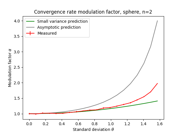
Refer to caption
Refer to caption
Refer to caption
Figure 4: Predicted (green curve) versus measured modulation factor α(n,θ)=nVar(n,θ)/θ2𝛼𝑛𝜃𝑛Var𝑛𝜃superscript𝜃2\alpha(n,\theta)=n\text{Var}(n,\theta)/\theta^{2} on the speed of convergence of the empirical Fréchet mean to the population Fréchet mean on the sphere 𝒮2subscript𝒮2{\cal S}_{2}, computed with N=5000𝑁5000N=5000 drawings to approximate the expectation for a number of samples n=2𝑛2n=2, n=4𝑛4n=4 and n=10𝑛10n=10 to n=100𝑛100n=100.

Results are plotted in Figure 4 for several values of n𝑛n and compared to the value predicted by our non-asymptotic high concentration formula Eq.(21) (green curve) and by the asymptotic CLT formula Eq.(22) (grey curve). We see that the non-asymptotic high concentration expansion closely predicts the normalized modulation factor for θ<0.8rad𝜃0.8𝑟𝑎𝑑\theta<0.8rad, whatever the number of samples. Above this value, the neglected terms in O(θ5)𝑂superscript𝜃5O(\theta^{5}) take the lead and increase to a maximum which depends on how close we are to θ=π/2𝜃𝜋2\theta=\pi/2. In this formula, the influence of the number n𝑛n of sample points is visible for a very small value, but disappears for 5 to 10 points both in the predicted and measured modulation factors (right of Fig.4). For a small number of samples, the asymptotic CLT formula is significantly overestimating the modulation factor for a large range of values of θ𝜃\theta, while is become a very good predictor on almost all the range of values for n10𝑛10n\geq 10.

Very similar results are obtained for a uniform distribution on the hypersphere of radius θ𝜃\theta on the sphere 𝒮3subscript𝒮3{\cal S}_{3} around the north pole (0,0,0,1)0001(0,0,0,1) as shown in Fig. 5 and in higher dimensions. The more we increase the dimension, the more the asymptotic BP-CLT is overestimating the modulation factor for a small number of samples. However, the asymptotic approximation remains quite good for a large number of samples even close to θ=π/2𝜃𝜋2\theta=\pi/2.

Refer to caption
Refer to caption
Refer to caption
Figure 5: Predicted (green curve) versus measured modulation factor α(n,θ)=nVar(n,θ)/θ2𝛼𝑛𝜃𝑛Var𝑛𝜃superscript𝜃2\alpha(n,\theta)=n\text{Var}(n,\theta)/\theta^{2} on the speed of convergence of the empirical Fréchet mean to the population Fréchet mean on the sphere 𝒮3subscript𝒮3{\cal S}_{3}, computed with N=5000𝑁5000N=5000 drawings to approximate the expectation for a number of samples n=2𝑛2n=2, n=4𝑛4n=4 and n=10𝑛10n=10 to n=100𝑛100n=100.

7.5 Experiments on the hyperbolic space

A similar experiment can be made on the hyperbolic space 3subscript3\mathbb{H}_{3}. We consider the positive sheet (t>0𝑡0t>0) of the hyperboloid of equation x2+y2+z2t2=1superscript𝑥2superscript𝑦2superscript𝑧2superscript𝑡21x^{2}+y^{2}+z^{2}-t^{2}=-1 embedded in 4superscript4\mathbb{R}^{4}. Using the pseudo-metric (x,y,z,t)2=x2+y2+z2t2subscriptsuperscriptnorm𝑥𝑦𝑧𝑡2superscript𝑥2superscript𝑦2superscript𝑧2superscript𝑡2\|(x,y,z,t)\|^{2}_{*}=x^{2}+y^{2}+z^{2}-t^{2}, the hyperbolic space 3subscript3\mathbb{H}_{3} can be seen as the pseudo-sphere of radius -1 in the Minkowski space 3,1superscript31\mathbb{R}^{3,1}. With these conventions, geodesics are the trace of 2-planes passing through the origin and the Riemannian distance is the arc-length d(x,y)=arccosh(x|y)𝑑𝑥𝑦arccoshsubscriptinner-product𝑥𝑦d(x,y)=\text{arccosh}(-\left<\>x\>\left|\>y\right.\right>_{*}).

As in the previous case, we consider a uniform distribution on the hypersphere of radius θ+𝜃superscript\theta\in\mathbb{R}^{+} centered at (0,0,0,1)0001(0,0,0,1) in 3subscript3\mathbb{H}_{3}. In the embedding space 4superscript4\mathbb{R}^{4}, this hypersphere in 3subscript3\mathbb{H}_{3} is the intersection of the hyperplane t=coshθ𝑡𝜃t=\cosh\theta with the hyperboloid. It is thus simply a sphere of radius sinhθ𝜃\sinh\theta in this hyperplane. A uniform distribution on the hypersphere is thus easily obtained from a uniform distribution on the 3-sphere. Because the hyperbolic space 3subscript3\mathbb{H}_{3} has negative curvature and is Hadamard, there exists a unique Fréchet mean which is the center of the hypersphere x¯=(0,0,0,1)¯𝑥0001\bar{x}=(0,0,0,1). However, the negative curvature may also cause the classical Gauss-Newton gradient descent algorithm to diverge when the variance of the distribution is large (see [7] for an example on SPD matrices with the affine-invariant metric). The algorithm may simply be modified with an adaptive Levenberg-Marquardt time-step τ<1𝜏1\tau<1 in the formula x¯t+1=expx¯t(τ1nilogx¯t(xi))superscript¯𝑥𝑡1subscriptsuperscript¯𝑥𝑡𝜏1𝑛subscript𝑖subscriptsuperscript¯𝑥𝑡subscript𝑥𝑖\bar{x}^{t+1}=\exp_{\bar{x}^{t}}(\tau\frac{1}{n}\sum_{i}\log_{\bar{x}^{t}}(x_{i})).

We draw an empirical distribution of n𝑛n points uniformly sampled on the hypersphere of radius θ𝜃\theta. We compute the square geodesic distance between the pole x¯=(0,0,0,1)¯𝑥0001\bar{x}=(0,0,0,1) and the obtained empirical Fréchet mean x¯nsubscript¯𝑥𝑛\bar{x}_{n}of this sample. Averaging this value for a large number N𝑁N of repeated random sampling allows us to compute a stochastic integral of the variance at the Fréchet mean Var(n,θ)=Var(x¯n)Var𝑛𝜃Varsubscript¯𝑥𝑛\text{Var}(n,\theta)=\text{Var}(\bar{x}_{n}). Finally, we compute the normalized modulation factor α(n,θ)=nVar(n,θ)/θ2𝛼𝑛𝜃𝑛Var𝑛𝜃superscript𝜃2\alpha(n,\theta)=n\text{Var}(n,\theta)/\theta^{2} which indicates how the rate of convergence differs from the Euclidean case.
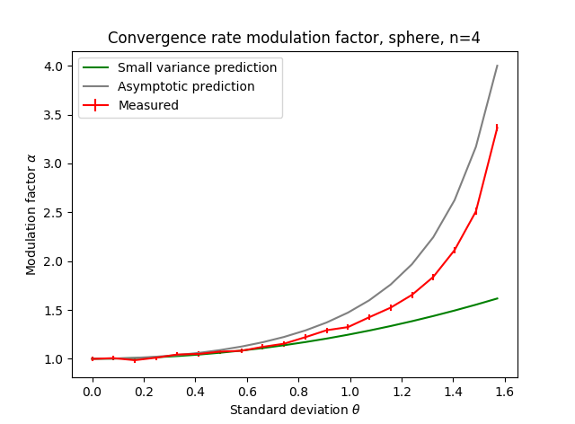
Refer to caption
Refer to caption
Refer to caption
Figure 6: Predicted (green curve) versus measured modulation factor α(n,θ)=nVar(n,θ)/θ2𝛼𝑛𝜃𝑛Var𝑛𝜃superscript𝜃2\alpha(n,\theta)=n\text{Var}(n,\theta)/\theta^{2} on the speed of convergence of the empirical Fréchet mean to the population Fréchet mean on the hyperbolic space 3subscript3\mathbb{H}_{3}, computed with N=5000𝑁5000N=5000 drawings to approximate the expectation. Top raw: curve along θ=[0;5]𝜃05\theta=[0;5] for a number of samples n=2𝑛2n=2, n=5𝑛5n=5 and n=10𝑛10n=10 to n=100𝑛100n=100.

Results are displayed in Figure 6 for several values of θ𝜃\theta and n𝑛n (red curve) and compared to the value predicted by our non-asymptotic high concentration formula Eq.(21) (green curve) and by the asymptotic CLT formula Eq.(22) (grey curve). We see that the non-asymptotic high concentration expansion closely predicts the normalized modulation factor for θ<1𝜃1\theta<1, whatever the number of samples. Above this value, the terms in O(θ5)𝑂superscript𝜃5O(\theta^{5}) neglected in the Taylor expansion take the lead and the formula gets useless. The asymptotic CLT formula is significantly underestimating the modulation factor for the whole range of values of θ𝜃\theta for a small number of samples. It becomes a very good predictor on all the range of values for n10𝑛10n\geq 10. In the presented experiments, we limited the radius θ𝜃\theta to 6 for visualization purposes. However, we have observed a modulating factor as low as α=0.01𝛼0.01\alpha=0.01 for θ=15𝜃15\theta=15 (i.e. an acceleration of the convergence by two orders of magnitude with respect to the Euclidean case) for two points. It is also interesting to notice that the number n𝑛n of points in the sample has a very limited influence on the modulation factor for n10𝑛10n\geq 10: the main factor is visibly the variance θ2superscript𝜃2\theta^{2} of the sample.

8 Discussion

We have derived in this paper a new type of approximation of the moments of the empirical mean x¯nsubscript¯𝑥𝑛\bar{x}_{n} of an IID n𝑛n-sample of a sufficiently concentrated distribution on a Riemannian and affine connection manifolds. This high concentration expansion of the moments of the empirical mean shows a bias in 1/n1𝑛1/n which is directly proportional to the gradient of the curvature tensor contracted twice with the covariance matrix. This unexpected bias, apparently never described before, is important in the small sample regime. The high concentration expansion of the covariance matrix of the empirical mean has also a curvature correction term modulating (accelerating or decelerating) the convergence with respect to the Euclidean case. The main variable controlling the modulation is the covariance-curvature tensor R(,)𝔐2𝑅subscript𝔐2R({\scriptscriptstyle{\bullet}},{\scriptscriptstyle{\circ}}){\scriptscriptstyle{\bullet}}\>\overset{\scriptscriptstyle{\bullet}}{{\scriptscriptstyle{\bullet}}}\>{\mathfrak{M}}_{2} (the matrix Aji=Rklji𝔐2klsubscriptsuperscript𝐴𝑖𝑗subscriptsuperscript𝑅𝑖𝑘𝑙𝑗superscriptsubscript𝔐2𝑘𝑙A^{i}_{j}=R^{i}_{klj}{\mathfrak{M}}_{2}^{kl} in coordinates).

Our new high-concentration expansion is valid in the small sample regime. Thus, it is a useful complement to the Bhattacharya-Patrangenaru central-limit theorem, which gives an asymptotic expansion for a large number of samples. With our notations, the BP-CLT states that the empirical mean x¯nsubscript¯𝑥𝑛\bar{x}_{n} converges in expectation to the true mean x¯¯𝑥\bar{x} with a rate of at least 1/n1𝑛1/\sqrt{n} and with covariance matrix (at the true mean) Cov(x¯n)=1n4H¯(-1)𝔐2H¯(-1)Covsubscript¯𝑥𝑛1𝑛4superscript¯𝐻(-1)subscript𝔐2superscript¯𝐻(-1)\text{Cov}(\bar{x}_{n})=\frac{1}{n}4\bar{H}^{\text{\tiny(-1)}}{\mathfrak{M}}_{2}\bar{H}^{\text{\tiny(-1)}}, where H¯¯𝐻\bar{H} is the expected Hessian of the Riemannian square distance (according to the distribution). The high concentration expansion of this expected Hessian H¯=2Id23R(,)𝔐2+O(ε3)¯𝐻2Id23𝑅subscript𝔐2𝑂superscript𝜀3\bar{H}=2\>\mathrm{Id}-\frac{2}{3}R({\scriptscriptstyle{\bullet}},{\scriptscriptstyle{\circ}}){\scriptscriptstyle{\bullet}}\>\overset{\scriptscriptstyle{\bullet}}{{\scriptscriptstyle{\bullet}}}\>{\mathfrak{M}}_{2}+O(\varepsilon^{3}) is controlled once again by the covariance-curvature tensor, as already observed in [33], so that both expansions are consistent in the high-concentration asymptotic regime.

In constant curvature spaces, we showed that both the asymptotic BP-CLT and the non-asymptotic high-concentration expansion predict a deviation of the decrease of the covariance of the empirical mean with respect to the Euclidean case. This modulation of the convergence speed can be encoded with a single multiplicative factor α𝛼\alpha which indicates that the variance of the Fréchet mean decreases faster in negatively curved space forms than in the Euclidean case, while it decreases more slowly in positive curvature space forms. The archetypal modulation factor goes to zero for an infinite negative curvature. This suggests that we could see here the beginning of the stickiness of the Fréchet mean described in stratified spaces. On the contrary, the modulation factor goes to infinity when we approach the limits of the Karcher & Kendall concentration conditions with a uniform distribution on the equator of the sphere, for which the Fréchet mean is not a single point anymore. Although an explicit formula has previously been established for the BP-CLT in space forms, it seems that the interpretation of the influence of the curvature of empirical means got unnoticed so far.

Acknowledgements.

This project has received funding from the European Research Council (ERC) under the European Union’s Horizon 2020 research and innovation program (grant G-Statistics agreement No 786854). Sincere thanks Yann Thanwerdas and Nicolas Guigui for their proofreading of the manuscript.

Appendix A Equivalence of notations with Darling’s paper

In the process of establishing the foundations of Kalman filtering on manifolds [13], Darling derived a coordinate free approximation of the exponential barycenter estimation in a manifold. The work of this research report was apparently unpublished in a journal, which is very unfortunate as it got completely unnoticed.

His Exponential Barycenter Formula Eq.(26) (Section 3.2, p.12) actually corresponds to the order 3 of our formula Eq.(12). However, the 4th order necessary to see that there is a bias on the empirical mean was not derived. Rephrased in the notations of this, his formula reads

logx(x¯)=𝔐113Rijk𝔐1i𝔐2jk+O(ε4).subscript𝑥¯𝑥subscript𝔐113subscript𝑅𝑖𝑗𝑘superscriptsubscript𝔐1𝑖superscriptsubscript𝔐2𝑗𝑘𝑂superscript𝜀4\log_{x}(\bar{x})={\mathfrak{M}}_{1}-\frac{1}{3}R_{ijk}{\mathfrak{M}}_{1}^{i}{\mathfrak{M}}_{2}^{jk}+O(\varepsilon^{4}).

However, the convention for the sign of the Riemannian curvature tensor is the opposite of ours. Indeed, Darling defines

R(u,v)w=DΓ(v)(wu)DΓ(u)(wv)+Γ(Γ(wu)v)Γ(Γ(wv)u).𝑅𝑢𝑣𝑤𝐷Γ𝑣tensor-product𝑤𝑢𝐷Γ𝑢tensor-product𝑤𝑣Γtensor-productΓtensor-product𝑤𝑢𝑣Γtensor-productΓtensor-product𝑤𝑣𝑢R(u,v)w=D\Gamma(v)(w\otimes u)-D\Gamma(u)(w\otimes v)+\Gamma(\Gamma(w\otimes u)\otimes v)-\Gamma(\Gamma(w\otimes v)\otimes u).

Taking w=b𝑤subscript𝑏w=\partial_{b}, u=c𝑢subscript𝑐u=\partial_{c}, v=d𝑣subscript𝑑v=\partial_{d}, we obtain

R(c,d)b=dΓbccΓbd+ΓedΓbceΓecΓbde.𝑅subscript𝑐subscript𝑑subscript𝑏subscript𝑑subscriptΓ𝑏𝑐subscript𝑐subscriptΓ𝑏𝑑subscriptΓ𝑒𝑑subscriptsuperscriptΓ𝑒𝑏𝑐subscriptΓ𝑒𝑐subscriptsuperscriptΓ𝑒𝑏𝑑R(\partial_{c},\partial_{d})\partial_{b}=\partial_{d}\Gamma_{bc}-\partial_{c}\Gamma_{bd}+\Gamma_{ed}\Gamma^{e}_{bc}-\Gamma_{ec}\Gamma^{e}_{bd}.

Given that the connection is torsion-free, we have Γij=ΓjisubscriptΓ𝑖𝑗subscriptΓ𝑗𝑖\Gamma_{ij}=\Gamma_{ji}, and we see that this formula is the opposite convention of the one used in this paper in Eq.2.

The index of the Riemannian curvature tensor also differ from ours. Here Rijk=R(i,j)ksubscript𝑅𝑖𝑗𝑘𝑅subscript𝑖subscript𝑗subscript𝑘R_{ijk}=R(\partial_{i},\partial_{j})\partial_{k}, so that Rijk𝔐1i𝔐2jk=R(𝔐1,)𝔐2subscript𝑅𝑖𝑗𝑘superscriptsubscript𝔐1𝑖superscriptsubscript𝔐2𝑗𝑘𝑅subscript𝔐1subscript𝔐2R_{ijk}{\mathfrak{M}}_{1}^{i}{\mathfrak{M}}_{2}^{jk}=R({\mathfrak{M}}_{1},{\scriptscriptstyle{\bullet}}){\scriptscriptstyle{\bullet}}\>\overset{\scriptscriptstyle{\bullet}}{{\scriptscriptstyle{\bullet}}}\>{\mathfrak{M}}_{2}. Taking the opposite due to the curvature convention correctly give the term R(,𝔐1)𝔐2𝑅subscript𝔐1subscript𝔐2R({\scriptscriptstyle{\bullet}},{\mathfrak{M}}_{1}){\scriptscriptstyle{\bullet}}\>\overset{\scriptscriptstyle{\bullet}}{{\scriptscriptstyle{\bullet}}}\>{\mathfrak{M}}_{2} of our formula Eq.(12).

References

  • [1] Bijan Afsari. Riemannian Lpsuperscript𝐿𝑝L^{p} center of mass: Existence, uniqueness, and convexity. Proceedings of the American Mathematical Society, 139(02):655–673, February 2011.
  • [2] Marc Arnaudon and Xue-Mei Li. Barycenters of measures transported by stochastic flows. The Annals of Probability, 33(4):1509–1543, July 2005.
  • [3] Bojan Basrak. Limit theorems for the inductive mean on metric trees. Journal of Applied Probability, 47(4):1136–1149, December 2010.
  • [4] Marcel Berger. A Panoramic View of Riemannian Geometry. Springer Berlin Heidelberg, Berlin, Heidelberg, 2003.
  • [5] Abhishek Bhattacharya and Rabi Bhattacharya. Statistics on Riemannian manifolds: asymptotic distribution and curvature. Proceedings of the American Mathematical Society, 136(8):2959–2967, 2008.
  • [6] Rabi Bhattacharya and Vic Patrangenaru. Large sample theory of intrinsic and extrinsic sample means on manifolds-II. The Annals of Statistics, 33(3):1225–1259, June 2005.
  • [7] Dario A. Bini and Bruno Iannazzo. Computing the Karcher mean of symmetric positive definite matrices. Linear Algebra and its Applications, 438(4):1700–1710, February 2013.
  • [8] Leo Brewin. Riemann normal coordinate expansions using Cadabra. Classical and Quantum Gravity, 26(17):175017, September 2009.
  • [9] Peter Buser and Hermann Karcher. Gromov’s almost flat manifolds. Number 81 in Astérisque. Société mathématique de France, 1981.
  • [10] Samuel R. Buss and Jay P. Fillmore. Spherical Averages and Applications to Spherical Splines and Interpolation. ACM Trans. Graph., 20(2):95–126, April 2001.
  • [11] Élie Cartan. Leçons sur la géométrie des espaces de Riemann. Gauthier-Villars, Paris, France, 1928.
  • [12] Élie Cartan. Groupes simples clos et ouverts et géométrie riemannienne. Journal de Mathématiques Pures et Appliquées, 9e série(tome 8):1–34, 1929.
  • [13] Richard William Ramsay Darling. Geometrically Intrinsic Nonlinear Recursive Filters II: Foundations. Electronic Journal of Probability, 5:1–18, 2000. arXiv: math/9809029.
  • [14] Manfredo Perdigao do Carmo. Riemannian geometry. Mathematics. Theory & Applications. Birkhäuser, Boston, 1992.
  • [15] Benjamin Eltzner and Stephan F. Huckemann. A Smeary Central Limit Theorem for Manifolds with Application to High Dimensional Spheres. arXiv:1801.06581 [math, stat], January 2018. arXiv: 1801.06581.
  • [16] M. Emery and G. Mokobodzki. Sur le barycentre d’une probabilité dans une variété. In Séminaire de Probabilités XXV, volume 1485, pages 220–233. Springer Berlin Heidelberg, Berlin, Heidelberg, 1991.
  • [17] Maurice Fréchet. Valeurs moyennes attachées a un triangle aléatoire. La revue scientifique, Fascicule 10:475–482, December 1943.
  • [18] Maurice Fréchet. Les éléments aléatoires de nature quelconque dans un espace distancié. Annales de l’Institut Henri Poincaré, 10:215–310, 1948.
  • [19] A V Gavrilov. Algebraic Properties of Covariant Derivative and Composition of Exponential Maps. Math. Tr., 9(1):3–20, 2006. English version in Siberian Advances in Mathematics, 2006, 16:3, 54-70.
  • [20] A. V. Gavrilov. The double exponential map and covariant derivation. Siberian Mathematical Journal, 48(1):56–61, January 2007.
  • [21] Karsten Grove and Hermann Karcher. How to conjugate C1-close group actions. Mathematische Zeitschrift, 132(1):11–20, March 1973.
  • [22] Susan Holmes. Personnal communication.
  • [23] Thomas Hotz, Stephan Huckemann, Huiling Le, J. S. Marron, Jonathan C. Mattingly, Ezra Miller, James Nolen, Megan Owen, Vic Patrangenaru, and Sean Skwerer. Sticky central limit theorems on open books. The Annals of Applied Probability, 23(6):2238–2258, December 2013.
  • [24] H. Karcher. Riemannian center of mass and mollifier smoothing. Communications on Pure and Applied Mathematics, 30(5):509–541, September 1977.
  • [25] Hermann Karcher. Riemannian Center of Mass and so called Karcher mean. arXiv:1407.2087 [math], July 2014.
  • [26] Wilfrid S. Kendall and Huiling Le. Limit theorems for empirical Fréchet means of independent and non-identically distributed manifold-valued random variables. Brazilian Journal of Probability and Statistics, 25(3):323–352, November 2011.
  • [27] W.S. Kendall. Probability, convexity, and harmonic maps with small image I: uniqueness and fine existence. Proc. London Math. Soc., 61(2):371–406, 1990.
  • [28] Huiling Le. Locating Fréchet Means with Application to Shape Spaces. Advances in Applied Probability, 33(2):324–338, 2001.
  • [29] Huiling Le. Estimation of Riemannian barycenters. LMS J. Comput. Math., 7:193–200, 2004.
  • [30] John M. Lee. Riemannian manifolds: an introduction to curvature. Number 176 in Graduate texts in mathematics. Springer, New York, 1997.
  • [31] Charles W. Misner, Kip S. Thorne, and John Archibald Wheeler. Gravitation. W. H. Freeman, San Francisco, 1973.
  • [32] Barrett O’Neill. Semi-Riemannian geometry: with applications to relativity. Number 103 in Pure and applied mathematics. Academic Press, New York, 1983.
  • [33] Xavier Pennec. Barycentric subspace analysis on manifolds. Annals of Statistics, 46(6A):2711–2746, 2018.
  • [34] M. M Postnikov. Geometry VI: Riemannian geometry. Springer, Berlin, 2010.
  • [35] M. Spivak. Differential Geometry, volume 1. Publish or Perish, Inc., 2nd edition, 1979.
  • [36] Le Yang. Riemannian median and its estimation. LMS Journal of Computation and Mathematics, 13:461–479, December 2010.
  • [37] Herbert Ziezold. On Expected Figures and a Strong Law of Large Numbers for Random Elements in Quasi-Metric Spaces. In J. Kožešnik, editor, Transactions of the Seventh Prague Conference on Information Theory, Statistical Decision Functions, Random Processes and of the 1974 European Meeting of Statisticians, number 7A, pages 591–602. Springer Netherlands, 1977.