Target Encirclement with any Smooth Pattern Using Range-only Measurements

Fei Dong dongf17@mails.tsinghua.edu.cn    Keyou You\corauthrefcor youky@tsinghua.edu.cn    Shiji Song shijis@tsinghua.edu.cn Department of Automation and BNRist, Tsinghua University, Beijing, 100084, China.
Abstract

This paper proposes a coordinate-free controller to drive a mobile robot to encircle a target at unknown position by only using range measurements. Different from the existing works, a backstepping based controller is proposed to encircle the target with zero steady-state error for any desired smooth pattern. Moreover, we show its asymptotic exponential convergence under a fixed set of control parameters, which are independent of the initial distance to the target. The effectiveness and advantages of the proposed controller are validated via simulations.

keywords:
Target encirclement, backstepping control, circumnavigation, range-only measurements.
thanks: This work was supported in part by the National Natural Science Foundation of China under Grant 61722308 and in part by the National Key Research and Development Program of China under Grant 2016YFC0300801.

, , \corauth[cor]Corresponding author

1 Introduction

Target tracking with robots has been widely applied in both military and civilian fields, such as border patrol, convey protection, and aerial surveillance, and has attracted considerable research attention in decades. One of the tracking patterns is target encirclement (Marasco et al., 2012), which requires that a tracking robot encloses the target with flexible commands to neutralize the target by restricting its movement. Particularly, circumnavigation refers to that the robot exactly slides on a circle centered at the target (Shames et al., 2012; Matveev et al., 2011). Many works have focused on this problem, see e.g., Frew et al. (2007); Deghat et al. (2014); Hafez et al. (2014); Cao (2015); Zhang et al. (2017); Xiao & Lu (2017); Yu & Liu (2017) and references therein. However, their controllers cannot be applied to the target encirclement of this work.

If the states (position, velocity, course, etc.) of both the robot and target are available, a Lyapunov guidance vector fields method is proposed by Lawrence (2003) and adopted in Frew et al. (2008). Moreover, both the backstepping control method and the sliding mode control method have been introduced in Jiang & Nijmeijer (1997) and Lee et al. (2013), respectively. Clearly, they are coordinate-based and cannot be applied in the GPS-denied environment.

If the robot state is available but the target state is unknown, e.g., the target is an intruder, the target position can be estimated based on sensor measurements, such as range-only (Shames et al., 2012), bearing-only (Deghat et al., 2014; Zheng et al., 2015), or received signal strength (Hu et al., 2011). For a stationary target, an adaptive localization algorithm is devised using range-only measurements in Shames et al. (2012). By using a single vision camera, a vision-based motion estimator and an extended Kalman filter are designed in Dobrokhodov et al. (2008) and Zhang & Liu (2010), respectively. Note that it is impossible to locate the target if the robot state is unknown.

If neither the robot state nor the target position is available, e.g., the robot is an underwater or indoor vehicle, this problem becomes much more difficult. A sliding mode approach is proposed in Matveev et al. (2011) to solve the circumnavigation problem. Although the chattering phenomenon can be eliminated or reduced, their approach cannot achieve zero steady-state. Besides, it requires a particular assumption that the initial position of the robot is sufficiently far away from the target. A range-only controller is devised in Milutinovic et al. (2014); Milutinović et al. (2017), whose control parameters strongly depend on the initial distance to the target. In addition, Cao (2015) introduces a geometrical guidance law, whose idea is to drive the robot towards the tangent point of an auxiliary circle. However, this method involves the computation of trigonometric and inverse trigonometric functions. Since there is no control input to the robot if it enters this auxiliary circle, this may result in large overshoots. To solve it, a switching idea is adopted in Zhang et al. (2017) where the switching is performed based on the tracking error.

Note that all the aforementioned range-only based controllers are only applicable to the circumnavigation problem of a stationary target. Clearly, this pattern cannot adapt to the time-varying/complicated environment, e.g. obstacle avoidance, circumnavigation of multiple targets, moving target, and etc. Thus, we are interested in the so-called target encirclement with smooth time-varying reference commands in this work. To this purpose, we propose a coordinate-free controller with range-only measurements by exploiting the backstepping control. In a preliminary version of this work (Dong & You, 2019), we have shown its effectiveness for the circumnavigation problem. For a time-varying reference command, our controller naturally contains its time derivative in the recursively backward process. Thus, our approach can guarantee global convergence and exponential stability with zero steady-state error. Moreover, the control parameters are independent of the initial state due to the use of a saturation function in the backstepping control. The effectiveness and advantages of the proposed controller are validated via simulations.

The rest of this paper is organized as follows. In Section 2, the problem under consideration is formulated in details. In Section 3, the proposed controller is given by exploiting the backstepping control method. In Section 4, we prove the stability and convergence of the proposed controller for the circumnavigation problem. Target encirclement with smooth time-varying commands is shown in Section 5. Simulations are included in Section 6, and some concluding remarks are drawn in Section 7.

2 Problem Formulation

Let 𝒑o:=[xo,yo]assignsubscript𝒑𝑜superscriptsubscript𝑥𝑜subscript𝑦𝑜\bm{p}_{o}:=[x_{o},y_{o}]^{\prime} be the unknown position of a stationary target and the dynamics of the robot is given by

𝒑˙(t)=vc[cosθ(t),sinθ(t)],θ˙(t)=u(t),formulae-sequence˙𝒑𝑡subscript𝑣𝑐superscript𝜃𝑡𝜃𝑡˙𝜃𝑡𝑢𝑡\begin{split}\dot{\bm{p}}(t)&=v_{c}[\cos\theta(t),\sin\theta(t)]^{\prime},\\ \dot{\theta}(t)&=u(t),\end{split} (1)

where 𝒑(t)2𝒑𝑡superscript2\bm{p}(t)\in\mathbb{R}^{2}, vcsubscript𝑣𝑐v_{c}, θ(t)𝜃𝑡\theta(t), and u(t)𝑢𝑡u(t) denote the position, constant linear speed, heading course, and angular speed of the robot, respectively.

Under mild conditions, the objective of this work is to design a proper controller u(t)𝑢𝑡u(t) by using range-only measurements

d(t):=𝒑(t)𝒑o2assign𝑑𝑡subscriptnorm𝒑𝑡subscript𝒑𝑜2\displaystyle d(t):=\|\bm{p}(t)-\bm{p}_{o}\|_{2}

such that the robot eventually encircles the target in the form of any given smooth pattern, which can be specified by a smooth reference signal r(t)𝑟𝑡r(t). That is,

limt|d(t)r(t)|=limt|d˙(t)r˙(t)|=0.subscript𝑡𝑑𝑡𝑟𝑡subscript𝑡˙𝑑𝑡˙𝑟𝑡0\lim_{t\rightarrow\infty}|d(t)-r(t)|=\lim_{t\rightarrow\infty}|\dot{d}(t)-\dot{r}(t)|=0. (2)

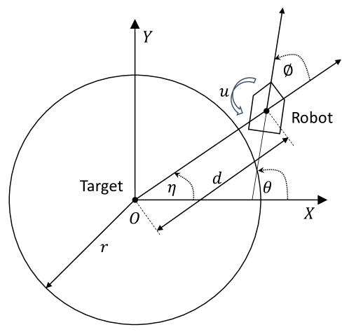
If r(t)rc𝑟𝑡subscript𝑟𝑐r(t)\equiv r_{c} is a positive constant, the desired pattern of the robot becomes an exact circle with the stationary target as its center. This is the celebrated circumnavigation problem in Cao (2015); Matveev et al. (2011) and see Fig. 1 for illustration. However, it is confirmed via simulations in Section 6 that their controllers cannot be directly extended to the case of time-varying r(t)𝑟𝑡r(t), which is the focus of this paper. Since the controller of this work only relies on range measurements between the robot and target, it is particularly useful in the GPS-denied environment and also substantially different from Dobrokhodov et al. (2008); Zhang & Liu (2010); Deghat et al. (2014); Xiao & Lu (2017), all of which need the GPS state information of the robot.

3 Controller Design

In this section, the controller is designed by using range-only measurements such that the distance d(t)𝑑𝑡d(t) to the target is able to track a smooth reference signal r(t)𝑟𝑡r(t) in the sense of (2). Our main idea is to exploit the advantage of the backstepping method, which is substantially different from Cao (2015); Matveev et al. (2011); Xiao & Lu (2017) and they can only solve the circumnavigation problem.

3.1 Range-only based controller for encircling

Let ϕ(t)(π,π]italic-ϕ𝑡𝜋𝜋\phi(t)\in(-\pi,\pi] be the angle formed by the direction from the target O𝑂O to the robot and the heading direction of the robot, see Fig. 1. By convention, the counterclockwise direction is set to be positive. Then, the robot dynamics in (1) can be transformed into

d˙(t)=vccosϕ(t),ϕ˙(t)=u(t)vcd(t)sinϕ(t).formulae-sequence˙𝑑𝑡subscript𝑣𝑐italic-ϕ𝑡˙italic-ϕ𝑡𝑢𝑡subscript𝑣𝑐𝑑𝑡italic-ϕ𝑡\begin{split}\dot{d}(t)&=v_{c}\cos\phi(t),\\ \dot{\phi}(t)&=u(t)-\frac{v_{c}}{d(t)}\sin\phi(t).\\ \end{split} (3)
Refer to caption
Figure 1: Target encirclement by a mobile robot.

From Fig. 1, we also have the relation that

ϕ(t)=θ(t)η(t),italic-ϕ𝑡𝜃𝑡𝜂𝑡\displaystyle\phi(t)=\theta(t)-\eta(t),

where η(t):=arctan((y(t)yo)/(x(t)xo))assign𝜂𝑡𝑦𝑡subscript𝑦𝑜𝑥𝑡subscript𝑥𝑜\eta(t):=\arctan((y(t)-y_{o})/(x(t)-x_{o})) is the angle between the direction from the target to the robot and the positive direction of x𝑥x-axis.

For a given smooth reference signal r(t)𝑟𝑡r(t), we exploit the backstepping method to design the following range-only based controller

u(t)=𝑢𝑡absent\displaystyle u(t)= vcα(t)d(t)+1vcα(t)×\displaystyle\frac{v_{c}\alpha(t)}{d(t)}+\frac{1}{v_{c}\alpha(t)}\times (4)
(k1(d˙(t)r˙(t)+k2sat(d(t)r(t)k3))r¨(t)),subscript𝑘1˙𝑑𝑡˙𝑟𝑡subscript𝑘2sat𝑑𝑡𝑟𝑡subscript𝑘3¨𝑟𝑡\displaystyle\left(k_{1}\left(\dot{d}(t)-\dot{r}(t)+k_{2}\text{sat}\big{(}\frac{d(t)-r(t)}{k_{3}}\big{)}\right)-\ddot{r}(t)\right),

where kisubscript𝑘𝑖k_{i}, i=1,2,3𝑖123i=1,2,3 are positive parameters, and

α(t)=|sinϕ(t)|=vc2(d˙(t))2/vc.𝛼𝑡italic-ϕ𝑡superscriptsubscript𝑣𝑐2superscript˙𝑑𝑡2subscript𝑣𝑐\alpha(t)=|\sin\phi(t)|=\sqrt{v_{c}^{2}-(\dot{d}(t))^{2}}/v_{c}.

The saturation function sat()sat\text{sat}(\cdot) is defined as

sat(η):={η,|η|<1,sgn(η),|η|1,assignsat𝜂cases𝜂𝜂1sgn𝜂𝜂1\displaystyle\text{sat}(\eta):=\begin{cases}\eta,&|\eta|<1,\\ \text{sgn}(\eta),&|\eta|\geq 1,\end{cases}

where sgn()sgn\text{sgn}(\cdot) is the standard signum function, and is utilized to ensure that all parameters work for any initial state of the robot. Moreover, we set d(t)=ε1𝑑𝑡subscript𝜀1d(t)=\varepsilon_{1} if d(t)ε1𝑑𝑡subscript𝜀1d(t)\leq\varepsilon_{1}, and α(t)=ε2𝛼𝑡subscript𝜀2\alpha(t)=\varepsilon_{2} if α(t)ε2𝛼𝑡subscript𝜀2\alpha(t)\leq\varepsilon_{2}, where εi,i=1,2formulae-sequencesubscript𝜀𝑖𝑖12\varepsilon_{i},i=1,2 are positive constant. Although it is extremely difficult to establish an explicit dependence, the tracking accuracy is positively related to k1subscript𝑘1k_{1}, and the convergence speed is mainly determined by k2subscript𝑘2k_{2} and k3subscript𝑘3k_{3}.

Moreover, one may employ a washout filter to track the derivative of d(t)𝑑𝑡d(t). That is, d˙(t)˙𝑑𝑡\dot{d}(t) in (4) is replaced by ξ(t)𝜉𝑡\xi(t), whose Laplace transform is given by

ξ(s)=hss+hd(s),𝜉𝑠𝑠𝑠𝑑𝑠\displaystyle\xi(s)=\frac{hs}{s+h}d(s), (5)

where s𝑠s is the Laplace operator, h>00h>0 is the filter parameter, and d(s)𝑑𝑠d(s) is the Laplace transform of the range-only input. Here the washout filter is used to damp the DC component of the range measurement d(t)𝑑𝑡d(t) (Lin et al., 2016). Noting that ξ(t)=d˙(t)𝜉𝑡˙𝑑𝑡\xi(t)=\dot{d}(t) if there is no measurement noise, and otherwise ξ(t)𝜉𝑡\xi(t) is a filtered version of d˙(t)˙𝑑𝑡\dot{d}(t). A similar idea of (5) has also been adopted in Guler & Fidan (2015).

3.2 Interpreting (4) from the backstepping control

Taking the derivative on both side of (3), we obtain that

d¨(t)=ϕ˙(t)vcsinϕ(t).¨𝑑𝑡˙italic-ϕ𝑡subscript𝑣𝑐italic-ϕ𝑡\displaystyle\ddot{d}(t)=-\dot{\phi}(t)v_{c}\sin\phi(t). (6)

Consider the following state vector of the robot

𝒙(t):=[x1(t),x2(t)]=[d(t),d˙(t)].assign𝒙𝑡superscriptsubscript𝑥1𝑡subscript𝑥2𝑡superscript𝑑𝑡˙𝑑𝑡\bm{x}(t):=[x_{1}(t),x_{2}(t)]^{\prime}=[d(t),\dot{d}(t)]^{\prime}. (7)

Then, it follows from (6) that

x˙1(t)=x2(t),x˙2(t)=f(𝒙(t))+g(𝒙(t))u(t),formulae-sequencesubscript˙𝑥1𝑡subscript𝑥2𝑡subscript˙𝑥2𝑡𝑓𝒙𝑡𝑔𝒙𝑡𝑢𝑡\begin{split}\dot{x}_{1}(t)&=x_{2}(t),\\ \dot{x}_{2}(t)&=f(\bm{x}(t))+g(\bm{x}(t))u(t),\\ \end{split} (8)

where the functions f𝑓f and g𝑔g are given by

f(𝒙(t))=vc2x1(t)sin2ϕ(t),g(𝒙(t))=vcsinϕ(t).formulae-sequence𝑓𝒙𝑡superscriptsubscript𝑣𝑐2subscript𝑥1𝑡superscript2italic-ϕ𝑡𝑔𝒙𝑡subscript𝑣𝑐italic-ϕ𝑡\begin{split}f(\bm{x}(t))&=\frac{v_{c}^{2}}{x_{1}(t)}\sin^{2}\phi(t),\\ g(\bm{x}(t))&=-v_{c}\sin\phi(t).\\ \end{split} (9)

Define an error vector 𝒆(t):=[e1(t),e2(t)]assign𝒆𝑡superscriptsubscript𝑒1𝑡subscript𝑒2𝑡\bm{e}(t):=[e_{1}(t),e_{2}(t)]^{\prime} by

e1(t):=x1(t)r(t),e2(t):=x2(t)s(t),formulae-sequenceassignsubscript𝑒1𝑡subscript𝑥1𝑡𝑟𝑡assignsubscript𝑒2𝑡subscript𝑥2𝑡𝑠𝑡\begin{split}e_{1}(t):=&x_{1}(t)-r(t),\\ e_{2}(t):=&x_{2}(t)-s(t),\\ \end{split} (10)

where s(t)𝑠𝑡s(t) is a virtual guidance command and is defined as

s(t):=c1e1(t)+r˙(t).assign𝑠𝑡subscript𝑐1subscript𝑒1𝑡˙𝑟𝑡\displaystyle s(t):=-c_{1}e_{1}(t)+\dot{r}(t). (11)

Here c1>0subscript𝑐10c_{1}>0 is a control parameter, and r˙(t)˙𝑟𝑡\dot{r}(t) is the derivative of the desired command r(t)𝑟𝑡r(t).

Consider the Lyapunov function candidate as

V1(e1)=12e12(t).subscript𝑉1subscript𝑒112superscriptsubscript𝑒12𝑡\displaystyle V_{1}(e_{1})=\frac{1}{2}e_{1}^{2}(t).

Taking the derivative of V1(e1)subscript𝑉1subscript𝑒1V_{1}(e_{1}), we have that

V˙1(e1)subscript˙𝑉1subscript𝑒1\displaystyle\dot{V}_{1}(e_{1}) =e1(t)e˙1(t)absentsubscript𝑒1𝑡subscript˙𝑒1𝑡\displaystyle=e_{1}(t)\dot{e}_{1}(t)
=c1e1(t)2+e1(t)e2(t).absentsubscript𝑐1subscript𝑒1superscript𝑡2subscript𝑒1𝑡subscript𝑒2𝑡\displaystyle=-c_{1}e_{1}(t)^{2}+e_{1}(t)e_{2}(t).

If e2(t)=0subscript𝑒2𝑡0e_{2}(t)=0, then V˙1(e1)0subscript˙𝑉1subscript𝑒10\dot{V}_{1}(e_{1})\leq 0 and x2(t)=s(t)subscript𝑥2𝑡𝑠𝑡x_{2}(t)=s(t). Moreover,

e˙1(t)=c1e1(t).subscript˙𝑒1𝑡subscript𝑐1subscript𝑒1𝑡\dot{e}_{1}(t)=-c_{1}e_{1}(t).

In this case, e1(t)subscript𝑒1𝑡e_{1}(t) exponentially converges to 00 as t𝑡t goes to infinity. Thus, it is sufficient to design a proper controller u(t)𝑢𝑡u(t) to asymptotically drive e2(t)subscript𝑒2𝑡e_{2}(t) to zero. A natural idea is to use a backstepping controller (Khalil, 2002; Jiang & Nijmeijer, 1997), i.e.,

u(t)=c2e2(t)+e1(t)+f(𝒙(t))s˙(t)g(𝒙(t)),𝑢𝑡subscript𝑐2subscript𝑒2𝑡subscript𝑒1𝑡𝑓𝒙𝑡˙𝑠𝑡𝑔𝒙𝑡\displaystyle u(t)=-\frac{c_{2}e_{2}(t)+e_{1}(t)+f(\bm{x}(t))-\dot{s}(t)}{g(\bm{x}(t))}, (12)

where c2>0subscript𝑐20c_{2}>0 is a positive parameter, and s˙(t)˙𝑠𝑡\dot{s}(t) is the derivative of the virtual command s(t)𝑠𝑡s(t).

To validate the controller in (12), consider the Lyapunov function candidate as

V2(𝒆)=V1(e1)+12e22(t).subscript𝑉2𝒆subscript𝑉1subscript𝑒112superscriptsubscript𝑒22𝑡\displaystyle V_{2}(\bm{e})=V_{1}(e_{1})+\frac{1}{2}e_{2}^{2}(t).

Taking derivative of V2(𝒆)subscript𝑉2𝒆V_{2}(\bm{e}) along with (8) leads to that

V˙2(𝒆)subscript˙𝑉2𝒆\displaystyle\dot{V}_{2}(\bm{e}) =e1(t)e˙1(t)+e2(t)e˙2(t)absentsubscript𝑒1𝑡subscript˙𝑒1𝑡subscript𝑒2𝑡subscript˙𝑒2𝑡\displaystyle=e_{1}(t)\dot{e}_{1}(t)+e_{2}(t)\dot{e}_{2}(t)
=e1(t)e˙1(t)+e2(t)(f(𝒙(t))+g(𝒙(t))u(t)s˙(t))absentsubscript𝑒1𝑡subscript˙𝑒1𝑡subscript𝑒2𝑡𝑓𝒙𝑡𝑔𝒙𝑡𝑢𝑡˙𝑠𝑡\displaystyle=e_{1}(t)\dot{e}_{1}(t)+e_{2}(t)\big{(}f(\bm{x}(t))+g(\bm{x}(t))u(t)-\dot{s}(t)\big{)}
=c1e12(t)c2e22(t)absentsubscript𝑐1superscriptsubscript𝑒12𝑡subscript𝑐2superscriptsubscript𝑒22𝑡\displaystyle=-c_{1}e_{1}^{2}(t)-c_{2}e_{2}^{2}(t)
0.absent0\displaystyle\leq 0.

Thus, V2(𝒆)subscript𝑉2𝒆V_{2}(\bm{e}) satisfies the following three conditions

  • Nonnegative: V2(𝒆)0subscript𝑉2𝒆0V_{2}(\bm{e})\geq 0, and V2(𝒆)=0subscript𝑉2𝒆0V_{2}(\bm{e})=0 if and only if 𝒆(t)=𝟎𝒆𝑡0\bm{e}(t)=\bm{0}.

  • Strictly decreasing: V˙2(𝒆)<0subscript˙𝑉2𝒆0\dot{V}_{2}(\bm{e})<0, 𝒆(t)𝟎for-all𝒆𝑡0\forall\bm{e}(t)\neq\bm{0}.

  • Radially unbounded: V2(𝒆)subscript𝑉2𝒆V_{2}(\bm{e})\rightarrow\infty, as 𝒆(t)2subscriptnorm𝒆𝑡2\|\bm{e}(t)\|_{2}\rightarrow\infty.

By Theorem 4.1 in Khalil (2002), the closed-loop system in (8) is asymptotically stable, i.e., d(t)r(t)𝑑𝑡𝑟𝑡d(t)\rightarrow r(t) and d˙(t)r˙(t)˙𝑑𝑡˙𝑟𝑡\dot{d}(t)\rightarrow\dot{r}(t) as t𝑡t\rightarrow\infty.

However, the backstepping controller in (12) further uses the information of the angle ϕ(t)italic-ϕ𝑡\phi(t). To solve it, we note from the dynamics in (3) that cosϕ(t)=x2(t)/vcitalic-ϕ𝑡subscript𝑥2𝑡subscript𝑣𝑐\cos\phi(t)=x_{2}(t)/v_{c}. Since sinϕ(t)=±1cos2ϕ(t)italic-ϕ𝑡plus-or-minus1superscript2italic-ϕ𝑡\sin\phi(t)=\pm\sqrt{1-\cos^{2}\phi(t)} and the sign of sinϕ(t)italic-ϕ𝑡\sin\phi(t) is unknown, we simply use α(t)=|sinϕ(t)|𝛼𝑡italic-ϕ𝑡\alpha(t)=|\sin\phi(t)| to replace it and the controller in (12) is modified as

u(t)𝑢𝑡\displaystyle u(t) =vcα(t)x1(t)1vcα(t)(c2e2(t)+e1(t)s˙(t))absentsubscript𝑣𝑐𝛼𝑡subscript𝑥1𝑡1subscript𝑣𝑐𝛼𝑡subscript𝑐2subscript𝑒2𝑡subscript𝑒1𝑡˙𝑠𝑡\displaystyle=-\frac{v_{c}\alpha(t)}{x_{1}(t)}-\frac{1}{v_{c}\alpha(t)}\big{(}c_{2}e_{2}(t)+e_{1}(t)-\dot{s}(t)\big{)}
=vcα(t)/x1(t)1/(vcα(t))×\displaystyle=-{v_{c}\alpha(t)}/{x_{1}(t)}-{1}/(v_{c}\alpha(t))\times
(c2e2(t)+e1(t)+c1x2(t)c1r˙(t)r¨(t))subscript𝑐2subscript𝑒2𝑡subscript𝑒1𝑡subscript𝑐1subscript𝑥2𝑡subscript𝑐1˙𝑟𝑡¨𝑟𝑡\displaystyle~{}~{}~{}~{}(c_{2}e_{2}(t)+e_{1}(t)+c_{1}x_{2}(t)-c_{1}\dot{r}(t)-\ddot{r}(t))
=vcα(t)/x1(t)1/(vcα(t))×\displaystyle=-{v_{c}\alpha(t)}/{x_{1}(t)}-{1}/(v_{c}\alpha(t))\times (13)
(k1(x2(t)r˙(t)+x1(t)r(t)k3)r¨(t)),subscript𝑘1subscript𝑥2𝑡˙𝑟𝑡subscript𝑥1𝑡𝑟𝑡subscript𝑘3¨𝑟𝑡\displaystyle~{}~{}~{}~{}{\left(k_{1}\left(x_{2}(t)-\dot{r}(t)+\displaystyle\frac{x_{1}(t)-r(t)}{k_{3}}\right)-\ddot{r}(t)\right)},

where k1=c1+c2subscript𝑘1subscript𝑐1subscript𝑐2k_{1}=c_{1}+c_{2}, and k3=(c1+c2)/(c1c2+1)subscript𝑘3subscript𝑐1subscript𝑐2subscript𝑐1subscript𝑐21k_{3}=(c_{1}+c_{2})/(c_{1}c_{2}+1).

When ϕ(t)[0,π]italic-ϕ𝑡0𝜋\phi(t)\in[0,\pi], it is clear that the controller in (3.2) is equivalent to that in (12). Thus, if there is a finite t1t0subscript𝑡1subscript𝑡0t_{1}\geq t_{0} such that ϕ(t)[0,π]italic-ϕ𝑡0𝜋\phi(t)\in[0,\pi], tt1for-all𝑡subscript𝑡1\forall t\geq t_{1} for any initial state ϕ(t0)italic-ϕsubscript𝑡0\phi(t_{0}), the controller in (3.2) can guarantee the global convergence.

To ensure the existence of such a finite t1subscript𝑡1t_{1}, the parameter k3subscript𝑘3k_{3} usually depends on the initial state of x1(t)subscript𝑥1𝑡x_{1}(t). Note that |x2(t)|vcsubscript𝑥2𝑡subscript𝑣𝑐|x_{2}(t)|\leq v_{c}, we adopt a saturation function to handle this problem. Then, the controller in (3.2) is further modified as (4).

In the sequel, we shall prove that the controller in (4) indeed drives the robot to encircle the target in the sense of (2).

3.3 Comparison with the literature

For the circumnavigation problem, i.e., r(t)rc𝑟𝑡subscript𝑟𝑐r(t)\equiv r_{c}, the proposed controller in (4) naturally reduces as

u(t)=vcα(t)d(t)+k1vcα(t)(d˙(t)+k2sat(d(t)rck3)).𝑢𝑡subscript𝑣𝑐𝛼𝑡𝑑𝑡subscript𝑘1subscript𝑣𝑐𝛼𝑡˙𝑑𝑡subscript𝑘2sat𝑑𝑡subscript𝑟𝑐subscript𝑘3\displaystyle u(t)=\frac{v_{c}\alpha(t)}{d(t)}+\frac{k_{1}}{v_{c}\alpha(t)}{\left(\dot{d}(t)+k_{2}\text{sat}(\frac{d(t)-r_{c}}{k_{3}})\right)}. (14)

When the robot is sliding on the desired orbit, i.e., d(t)=rc𝑑𝑡subscript𝑟𝑐d(t)=r_{c} and d˙(t)=0˙𝑑𝑡0\dot{d}(t)=0, the control output is exact vc/rcsubscript𝑣𝑐subscript𝑟𝑐v_{c}/r_{c}, which implies that there is no steady-state error. In contrast, the sliding mode controller in Matveev et al. (2011) cannot achieve zero steady-state error. Since this issue, Cao (2015) and Zhang et al. (2017) use switching controllers along with the distance error d(t)rc𝑑𝑡subscript𝑟𝑐d(t)-r_{c}. The idea of the geometrical method in Cao (2015) is to drive the robot towards the tangent point of an auxiliary circle, and there is no control when the robot enters the auxiliary circle, which may result in large overshoot.

In terms of the stability and convergence, our controller in (14) can ensure global convergence, and the control parameters are independent of the initial distance. In comparison, the sliding mode approach in Matveev et al. (2011) requires that the initial distance to the target is lager enough than the desired radius. The control parameters in Milutinović et al. (2017) are determined by solving a linear quadratic regulator (LQR) problem and depends on the initial distance.

Note that all methods mentioned above are concerned with the problem of target circumnavigation. Their methods cannot be directly extended to the case of smooth time-varying reference commands as confirmed in Section 6.

4 Target Encirclement with a Constant Reference Distance

As mentioned before, circumnavigation is a special case of target encirclement of this work, and is shown to be achieved under controller in (4) by setting r(t)rc𝑟𝑡subscript𝑟𝑐r(t)\equiv r_{c}.

4.1 Stability and convergence

Proposition 1.

Consider the encirclement system in (8) under the range-only based controller in (4). Let r(t)rc𝑟𝑡subscript𝑟𝑐r(t)\equiv r_{c} and 𝐱e:=[rc,0]assignsubscript𝐱𝑒superscriptsubscript𝑟𝑐0\bm{x}_{e}:=[r_{c},0]^{\prime}. If the controller parameters are selected to satisfy that

0<k2<vc,andk3=rcformulae-sequence0subscript𝑘2subscript𝑣𝑐andsubscript𝑘3subscript𝑟𝑐\displaystyle 0<k_{2}<v_{c},~{}\text{and}~{}k_{3}={r_{c}} (15)

there exists a finite t1>t0subscript𝑡1subscript𝑡0t_{1}>t_{0} such that

𝒙(t)𝒙eC𝒙(t1)𝒙eexp(ρ(tt1)),t>t1formulae-sequencenorm𝒙𝑡subscript𝒙𝑒𝐶norm𝒙subscript𝑡1subscript𝒙𝑒𝜌𝑡subscript𝑡1for-all𝑡subscript𝑡1\displaystyle\|\bm{x}(t)-\bm{x}_{e}\|\leq C\|\bm{x}(t_{1})-\bm{x}_{e}\|\exp\left(-\rho(t-t_{1})\right),\forall t>t_{1}

where 𝐱(t)𝐱𝑡\bm{x}(t) is defined in (7), ρ𝜌\rho and C𝐶C are two positive constants.

Thus, a proper set of parameters in (15) ensures that the robot completes the circumnavigation task for any initial state and the convergence is exponentially fast.

If 𝒙(t)=𝒙e𝒙𝑡subscript𝒙𝑒\bm{x}(t)=\bm{x}_{e}, the controller in (4) reduces to u(t)=vc/rc𝑢𝑡subscript𝑣𝑐subscript𝑟𝑐u(t)=v_{c}/r_{c}, which together with (3) implies that there is no steady-state error. In contrast, the sliding mode approach in Matveev et al. (2011) cannot achieve zero steady-state error.

4.2 Proof of Proposition 1

If ϕ(t)[0,π]italic-ϕ𝑡0𝜋\phi(t)\in[0,\pi], the controller in (3.2) is equivalent to that in (12), the effectiveness of which has been proved in Section 3.2. Thus, we first show that there must exist a finite time instant t1t0subscript𝑡1subscript𝑡0t_{1}\geq t_{0} such that ϕ(t)[0,π],tt1formulae-sequenceitalic-ϕ𝑡0𝜋for-all𝑡subscript𝑡1\phi(t)\in[0,\pi],\forall t\geq t_{1} for any initial state, see Lemma 2. Then, the closed-loop system in (8) under (14) is shown to be asymptotically stable in Lemma 3 and exponentially stable in Lemma 4.

Lemma 2.

Under the conditions in Proposition 1, there must exist a finite time instant t1t0subscript𝑡1subscript𝑡0t_{1}\geq t_{0} such that ϕ(t)[0,π]italic-ϕ𝑡0𝜋\phi(t)\in[0,\pi], tt1for-all𝑡subscript𝑡1\forall t\geq t_{1}, for any initial state ϕ(t0)(π,π]italic-ϕsubscript𝑡0𝜋𝜋\phi(t_{0})\in(-\pi,\pi].

{pf}

We prove that (a) ϕ(t)[0,π]italic-ϕ𝑡0𝜋\phi(t)\in[0,\pi] for any tt0𝑡subscript𝑡0t\geq t_{0} if ϕ(t0)[0,π]italic-ϕsubscript𝑡00𝜋\phi(t_{0})\in[0,\pi] and (b) there exists a t1>t0subscript𝑡1subscript𝑡0t_{1}>t_{0} such that ϕ(t1)[0,π]italic-ϕsubscript𝑡10𝜋\phi(t_{1})\in[0,\pi] for any ϕ(t0)(π,0)italic-ϕsubscript𝑡0𝜋0\phi(t_{0})\in(-\pi,0).

Combining (3) with (14), we obtain that

ϕ˙(t)˙italic-ϕ𝑡\displaystyle\dot{\phi}(t) =vcα(t)d(t)+k1vcα(t)(d˙(t)+k2sat(d(t)rck3))absentsubscript𝑣𝑐𝛼𝑡𝑑𝑡subscript𝑘1subscript𝑣𝑐𝛼𝑡˙𝑑𝑡subscript𝑘2sat𝑑𝑡subscript𝑟𝑐subscript𝑘3\displaystyle=\frac{v_{c}\alpha(t)}{d(t)}+\frac{k_{1}}{v_{c}\alpha(t)}{\big{(}\dot{d}(t)+k_{2}\text{sat}(\frac{d(t)-r_{c}}{k_{3}})\big{)}}
vcd(t)sinϕ(t).subscript𝑣𝑐𝑑𝑡italic-ϕ𝑡\displaystyle-\frac{v_{c}}{d(t)}\sin\phi(t). (16)

To prove part (a), we just need to show that ϕ˙(t)>0˙italic-ϕ𝑡0\dot{\phi}(t)>0 if ϕ(t)=0italic-ϕ𝑡0\phi(t)=0, and ϕ˙(t)<0˙italic-ϕ𝑡0\dot{\phi}(t)<0 if ϕ(t)=πitalic-ϕ𝑡𝜋\phi(t)=\pi. If ϕ(t)=0italic-ϕ𝑡0\phi(t)=0, it follows from (4.2) that

ϕ˙(t)˙italic-ϕ𝑡\displaystyle\dot{\phi}(t) =(vcε2)1k1(vc+k2sat(d(t)rck3))absentsuperscriptsubscript𝑣𝑐subscript𝜀21subscript𝑘1subscript𝑣𝑐subscript𝑘2sat𝑑𝑡subscript𝑟𝑐subscript𝑘3\displaystyle=(v_{c}\varepsilon_{2})^{-1}k_{1}\left(v_{c}+k_{2}\text{sat}(\frac{d(t)-r_{c}}{k_{3}})\right)
(vcε2)1k1(vck2)>0,absentsuperscriptsubscript𝑣𝑐subscript𝜀21subscript𝑘1subscript𝑣𝑐subscript𝑘20\displaystyle\geq(v_{c}\varepsilon_{2})^{-1}k_{1}(v_{c}-k_{2})>0,

where the last inequality uses the fact that vc>k2subscript𝑣𝑐subscript𝑘2{v_{c}}>k_{2}. Similarly, ϕ(t)=πitalic-ϕ𝑡𝜋\phi(t)=\pi leads to that

ϕ˙(t)˙italic-ϕ𝑡\displaystyle\dot{\phi}(t) =(vcε2)1k1(vc+k2sat(d(t)rck3))absentsuperscriptsubscript𝑣𝑐subscript𝜀21subscript𝑘1subscript𝑣𝑐subscript𝑘2sat𝑑𝑡subscript𝑟𝑐subscript𝑘3\displaystyle=(v_{c}\varepsilon_{2})^{-1}k_{1}\left(-v_{c}+k_{2}\text{sat}(\frac{d(t)-r_{c}}{k_{3}})\right)
(vcε2)1k1(vc+k2)<0.absentsuperscriptsubscript𝑣𝑐subscript𝜀21subscript𝑘1subscript𝑣𝑐subscript𝑘20\displaystyle\leq(v_{c}\varepsilon_{2})^{-1}k_{1}(-v_{c}+k_{2})<0. (17)

To prove part (b), four cases in Fig. 2 are considered.

Refer to caption

Figure 2: States of the robot.

For the case in Fig. 2(a), i.e., d(t0)[rc,)𝑑subscript𝑡0subscript𝑟𝑐d(t_{0})\in[r_{c},\infty) and ϕ(t0)[π/2,0)italic-ϕsubscript𝑡0𝜋20\phi(t_{0})\in[-\pi/2,0), it follows from (4) and (4.2) that d˙(t0)0˙𝑑subscript𝑡00\dot{d}(t_{0})\geq 0 and ϕ˙(t0)>0˙italic-ϕsubscript𝑡00\dot{\phi}(t_{0})>0. Thus, there must exist a t>t0subscript𝑡subscript𝑡0t_{*}>t_{0} such that 0>ϕ(t)>π/20italic-ϕsubscript𝑡𝜋20>\phi(t_{*})>-\pi/2 and d˙(t)>0˙𝑑subscript𝑡0\dot{d}(t_{*})>0. This implies that d(t)>rc𝑑subscript𝑡subscript𝑟𝑐d(t_{*})>r_{c}, and

ϕ˙(t)˙italic-ϕsubscript𝑡\displaystyle\dot{\phi}(t_{*}) =k1vcsinϕ(t)(d˙(t)+k2sat(d(t)rck3))absentsubscript𝑘1subscript𝑣𝑐italic-ϕsubscript𝑡˙𝑑subscript𝑡subscript𝑘2sat𝑑subscript𝑡subscript𝑟𝑐subscript𝑘3\displaystyle=-\frac{k_{1}}{v_{c}\sin\phi(t_{*})}{\left(\dot{d}(t_{*})+k_{2}\text{sat}(\frac{d(t_{*})-r_{c}}{k_{3}})\right)}
2vcsinϕ(t)d(t)2subscript𝑣𝑐italic-ϕsubscript𝑡𝑑subscript𝑡\displaystyle~{}~{}~{}~{}-\frac{2v_{c}\sin\phi(t_{*})}{d(t_{*})}
>k1cotϕ(t)absentsubscript𝑘1italic-ϕsubscript𝑡\displaystyle>-{k_{1}}{\cot\phi(t_{*})}
>0.absent0\displaystyle>0.

Thus, ϕ(t)italic-ϕ𝑡\phi(t) will monotonically increase until ϕ(t1)0italic-ϕsubscript𝑡10\phi(t_{1})\geq 0 at some finite time instant t1subscript𝑡1t_{1}.

For the case in Fig. 2(b), i.e., d(t0)[rc,)𝑑subscript𝑡0subscript𝑟𝑐d(t_{0})\in[r_{c},\infty) and ϕ(t0)(π,π/2)italic-ϕsubscript𝑡0𝜋𝜋2\phi(t_{0})\in(-\pi,-\pi/2), it follows from (4.2) and (4.2) that

{ϕ˙(t)>0,ifϕ(t)=π/2,ϕ˙(t)<0,ifϕ(t)=π.cases˙italic-ϕ𝑡0ifitalic-ϕ𝑡𝜋2˙italic-ϕ𝑡0ifitalic-ϕ𝑡𝜋\displaystyle\begin{cases}\dot{\phi}(t)>0,&\text{if}~{}\phi(t)=-\pi/2,\\ \dot{\phi}(t)<0,&\text{if}~{}\phi(t)=-\pi.\end{cases}

In this case, there are three possible results after some finite time Δ>0Δ0\Delta>0: (i) ϕ(t0+Δ)<πitalic-ϕsubscript𝑡0Δ𝜋\phi(t_{0}+\Delta)<-\pi and d(t0+Δ)rc𝑑subscript𝑡0Δsubscript𝑟𝑐d(t_{0}+\Delta)\geq r_{c}, then part (b) is finished; (ii) ϕ(t0+Δ)>π/2italic-ϕsubscript𝑡0Δ𝜋2\phi(t_{0}+\Delta)>-\pi/2 and d(t0+Δ)rc𝑑subscript𝑡0Δsubscript𝑟𝑐d(t_{0}+\Delta)\geq r_{c}, which is the case in Fig. 2(a); (iii) d(t0+Δ)<rc𝑑subscript𝑡0Δsubscript𝑟𝑐d(t_{0}+\Delta)<r_{c} which is to be shown for the cases in Fig. 2(c) and (d).

For d(t0)(0,rc)𝑑subscript𝑡00subscript𝑟𝑐d(t_{0})\in(0,r_{c}), it contains both cases in Fig. 2(c) and (d). When ϕ(t)=π/2italic-ϕ𝑡𝜋2\phi(t)=-\pi/2, it follows from (4.2) that

ϕ˙(t)˙italic-ϕ𝑡\displaystyle\dot{\phi}(t) =2vcd(t)k1k2rcvc(d(t)rc)absent2subscript𝑣𝑐𝑑𝑡subscript𝑘1subscript𝑘2subscript𝑟𝑐subscript𝑣𝑐𝑑𝑡subscript𝑟𝑐\displaystyle=\frac{-2v_{c}}{d(t)}-\frac{k_{1}k_{2}}{r_{c}v_{c}}({d(t)-r_{c}}) (18)
=d2(t)+rcd(t)2rcvc2/(k1k2)rcvcd(t)/(k1k2).absentsuperscript𝑑2𝑡subscript𝑟𝑐𝑑𝑡2subscript𝑟𝑐superscriptsubscript𝑣𝑐2subscript𝑘1subscript𝑘2subscript𝑟𝑐subscript𝑣𝑐𝑑𝑡subscript𝑘1subscript𝑘2\displaystyle=\frac{-d^{2}(t)+r_{c}d(t)-{2r_{c}v_{c}^{2}}/{(k_{1}k_{2})}}{{r_{c}v_{c}d(t)}/{(k_{1}k_{2})}}. (19)

Note that the numerator in the last equality is quadratic in d(t)𝑑𝑡d(t). If k1k2<8vc2subscript𝑘1subscript𝑘28superscriptsubscript𝑣𝑐2k_{1}k_{2}<8v_{c}^{2}, then it can be easily verified that

rc24×2rcvc2k1k2<0superscriptsubscript𝑟𝑐242subscript𝑟𝑐superscriptsubscript𝑣𝑐2subscript𝑘1subscript𝑘20\displaystyle r_{c}^{2}-4\times\frac{2r_{c}v_{c}^{2}}{k_{1}k_{2}}<0

and ϕ˙(t)<0˙italic-ϕ𝑡0\dot{\phi}(t)<0 for ϕ(t)=π/2italic-ϕ𝑡𝜋2\phi(t)=-\pi/2 and any d(t)(0,rc)𝑑𝑡0subscript𝑟𝑐d(t)\in(0,r_{c}). If k1k28vc2subscript𝑘1subscript𝑘28superscriptsubscript𝑣𝑐2k_{1}k_{2}\geq 8v_{c}^{2}, there exists an equilibrium 𝒚~e:=[d,π/2]assignsubscript~𝒚𝑒superscriptsubscript𝑑𝜋2\tilde{\bm{y}}_{e}:=[d_{*},-\pi/2]^{\prime} such that ϕ˙(t)=0˙italic-ϕ𝑡0\dot{\phi}(t)=0, where d(0,rc)subscript𝑑0subscript𝑟𝑐d_{*}\in(0,r_{c}). However, this equilibrium 𝒚~esubscript~𝒚𝑒\tilde{\bm{y}}_{e} is unstable. To prove it, we define 𝒚(t):=[d(t),ϕ(t)]assign𝒚𝑡superscript𝑑𝑡italic-ϕ𝑡\bm{y}(t):=[d(t),\phi(t)]^{\prime} and linearize the closed-loop system in (3) around 𝒚~esubscript~𝒚𝑒\tilde{\bm{y}}_{e} as follows

𝒚˙(t)=F(𝒚(t)𝒚~e)˙𝒚𝑡𝐹𝒚𝑡subscript~𝒚𝑒\displaystyle\dot{\bm{y}}(t)=F(\bm{y}(t)-\tilde{\bm{y}}_{e})

where the Jacobian matrix F𝐹F is given by

F=[0vck1k2rcvc2vcd2k1].𝐹matrix0subscript𝑣𝑐subscript𝑘1subscript𝑘2subscript𝑟𝑐subscript𝑣𝑐2subscript𝑣𝑐superscriptsubscript𝑑2subscript𝑘1\displaystyle F=\begin{bmatrix}0&v_{c}\\ \displaystyle\frac{k_{1}k_{2}}{r_{c}v_{c}}-\frac{2v_{c}}{d_{*}^{2}}&k_{1}\end{bmatrix}.

It is clear that at least one eigenvalue of F𝐹F has positive real part, i.e., the equilibrium 𝒚~esubscript~𝒚𝑒\tilde{\bm{y}}_{e} is unstable. Thus, ϕ(t)italic-ϕ𝑡\phi(t) cannot converge to π/2𝜋2-\pi/2 for any d(t)(0,rc)𝑑𝑡0subscript𝑟𝑐d(t)\in(0,r_{c}).

Suppose that ϕ(t)italic-ϕ𝑡\phi(t) can stay in (π/2,0)𝜋20(-\pi/2,0) for all time, then we have d˙(t)>0˙𝑑𝑡0\dot{d}(t)>0 in light of (3). Together with the fact that ϕ(t)italic-ϕ𝑡\phi(t) cannot converge to π/2𝜋2-\pi/2 for any d(t)(0,rc)𝑑𝑡0subscript𝑟𝑐d(t)\in(0,r_{c}), there must exist some finite time Δ>0Δ0\Delta>0 such that d(t0+Δ)rc𝑑subscript𝑡0Δsubscript𝑟𝑐d(t_{0}+\Delta)\geq r_{c}, which is the case in Fig. 2(a).

Similarly, d(t)>0𝑑𝑡0d(t)>0 implies that ϕ(t)italic-ϕ𝑡\phi(t) cannot stay in (π,π/2)𝜋𝜋2(-\pi,-\pi/2) for all time.

Consequently, there must exist a finite t1subscript𝑡1t_{1} such that ϕ(t1)[0,π]italic-ϕsubscript𝑡10𝜋\phi(t_{1})\in[0,\pi] for any ϕ(t0)(π,0)italic-ϕsubscript𝑡0𝜋0\phi(t_{0})\in(-\pi,0).  

In virtue of Lemma 2, the controller in (3.2) is eventually equivalent to that in (12), whose effectiveness has been shown in Section 3.2.

Lemma 3.

Under the conditions in Proposition 1, the closed-loop system in (8) is asymptotically stable.

{pf}

In view of Lemma 2, it holds that ϕ(t)[0,π]italic-ϕ𝑡0𝜋\phi(t)\in[0,\pi] for any tt1𝑡subscript𝑡1t\geq t_{1}. By (4.2), we obtain that

ϕ˙(t)=k1vcsinϕ(t)(d˙(t)+k2sat(d(t)rck3)).˙italic-ϕ𝑡subscript𝑘1subscript𝑣𝑐italic-ϕ𝑡˙𝑑𝑡subscript𝑘2sat𝑑𝑡subscript𝑟𝑐subscript𝑘3\displaystyle\dot{\phi}(t)=\frac{k_{1}}{v_{c}\sin\phi(t)}{\left(\dot{d}(t)+k_{2}\text{sat}(\frac{d(t)-r_{c}}{k_{3}})\right)}. (20)

Consider the Lyapunov function candidate as

V3(𝒙)=k1k2rcx1(t)sat(τrck3)dτ+12x22(t).subscript𝑉3𝒙subscript𝑘1subscript𝑘2superscriptsubscriptsubscript𝑟𝑐subscript𝑥1𝑡sat𝜏subscript𝑟𝑐subscript𝑘3d𝜏12superscriptsubscript𝑥22𝑡\displaystyle V_{3}(\bm{x})=k_{1}k_{2}\int_{r_{c}}^{x_{1}(t)}{\text{sat}(\frac{\tau-r_{c}}{k_{3}})}\text{d}\tau+\frac{1}{2}x_{2}^{2}(t).

Taking the time derivative of V3(𝒙)subscript𝑉3𝒙V_{3}(\bm{x}) along with (6), (8) and (20) leads to that

V˙3(𝒙)subscript˙𝑉3𝒙\displaystyle\dot{V}_{3}(\bm{x}) =k1k2sat(x1(t)rck3)x2(t)+x2(t)x˙2(t)absentsubscript𝑘1subscript𝑘2satsubscript𝑥1𝑡subscript𝑟𝑐subscript𝑘3subscript𝑥2𝑡subscript𝑥2𝑡subscript˙𝑥2𝑡\displaystyle=k_{1}k_{2}{\text{sat}(\frac{x_{1}(t)-r_{c}}{k_{3}})}x_{2}(t)+x_{2}(t)\dot{x}_{2}(t)
=k1k2sat(x1(t)rck3)x2(t)absentsubscript𝑘1subscript𝑘2satsubscript𝑥1𝑡subscript𝑟𝑐subscript𝑘3subscript𝑥2𝑡\displaystyle=k_{1}k_{2}{\text{sat}(\frac{x_{1}(t)-r_{c}}{k_{3}})}x_{2}(t)
x2(t)(k1x2(t)+k1k2sat(x1(t)rck3))subscript𝑥2𝑡subscript𝑘1subscript𝑥2𝑡subscript𝑘1subscript𝑘2satsubscript𝑥1𝑡subscript𝑟𝑐subscript𝑘3\displaystyle~{}~{}~{}~{}-x_{2}(t)\left(k_{1}x_{2}(t)+k_{1}k_{2}\text{sat}(\frac{x_{1}(t)-r_{c}}{k_{3}})\right)
=k1x22(t)absentsubscript𝑘1superscriptsubscript𝑥22𝑡\displaystyle=-k_{1}x_{2}^{2}(t)
0.absent0\displaystyle\leq 0.

However, V˙3(𝒙)subscript˙𝑉3𝒙\dot{V}_{3}(\bm{x}) is not always negative definite, e.g., V˙3(𝒙)=0subscript˙𝑉3𝒙0\dot{V}_{3}(\bm{x})=0 for x2(t)=0subscript𝑥2𝑡0x_{2}(t)=0 and any x1(t)>0subscript𝑥1𝑡0x_{1}(t)>0. Let 𝒮:={𝒙|V˙3(𝒙)=0}assign𝒮conditional-set𝒙subscript˙𝑉3𝒙0\mathcal{S}:=\{\bm{x}|\dot{V}_{3}(\bm{x})=0\}. For any 𝒙0𝒮subscript𝒙0𝒮{\bm{x}}_{0}\in\mathcal{S} but 𝒙0𝒙esubscript𝒙0subscript𝒙𝑒{\bm{x}}_{0}\neq\bm{x}_{e}, it holds that

x˙2(t)|𝒙(t)=𝒙0=k1k2sat(x1(t)rck3)0.evaluated-atsubscript˙𝑥2𝑡𝒙𝑡subscript𝒙0subscript𝑘1subscript𝑘2satsubscript𝑥1𝑡subscript𝑟𝑐subscript𝑘30\displaystyle\dot{x}_{2}(t)|_{\bm{x}(t)={\bm{x}}_{0}}=k_{1}k_{2}\text{sat}\big{(}\frac{x_{1}(t)-r_{c}}{k_{3}}\big{)}\neq 0.

Thus, x2(t)subscript𝑥2𝑡x_{2}(t) cannot maintain the state 𝒙(t)=𝒙o𝒙𝑡subscript𝒙𝑜\bm{x}(t)=\bm{x}_{o}, i.e., 𝒙0subscript𝒙0{\bm{x}}_{0} cannot stay identically in 𝒮𝒮\mathcal{S}.

Moreover, V3(𝒙)subscript𝑉3𝒙V_{3}(\bm{x}) is nonnegative and radially unbounded. By the LaSalle’s invariance theorem (Khalil, 2002, Corollary 4.2), 𝒙e=[rc,0]subscript𝒙𝑒superscriptsubscript𝑟𝑐0\bm{x}_{e}=[r_{c},0]^{\prime} is an asymptotically stable equilibrium point of the closed-loop system in (8).  

If the initial position of the robot is far away from the target, i.e., d(t0)rck3much-greater-than𝑑subscript𝑡0subscript𝑟𝑐subscript𝑘3d(t_{0})-r_{c}\gg k_{3} and ϕ(t0)[0,π]italic-ϕsubscript𝑡00𝜋\phi(t_{0})\in[0,\pi]. It follows from (20) that

ϕ˙(t0)=k1vcsinϕ(t0)(vccosϕ(t0)+k2).˙italic-ϕsubscript𝑡0subscript𝑘1subscript𝑣𝑐italic-ϕsubscript𝑡0subscript𝑣𝑐italic-ϕsubscript𝑡0subscript𝑘2\displaystyle\dot{\phi}(t_{0})=\frac{k_{1}}{v_{c}\sin\phi(t_{0})}{\left(v_{c}\cos\phi(t_{0})+k_{2}\right)}. (21)

For simplicity, we define φ:=cos1(k2/vc).assign𝜑superscript1subscript𝑘2subscript𝑣𝑐\varphi:=\cos^{-1}(-k_{2}/v_{c}). If ϕ(t0)[0,φ)italic-ϕsubscript𝑡00𝜑\phi(t_{0})\in[0,\varphi), then ϕ˙(t0)>0˙italic-ϕsubscript𝑡00\dot{\phi}(t_{0})>0 according to (21). Hence, ϕ(t)italic-ϕ𝑡\phi(t) monotonically increases until ϕ(t)=φitalic-ϕsubscript𝑡𝜑\phi(t_{*})=\varphi at some finite time instant t>t0subscript𝑡subscript𝑡0t_{*}>t_{0}. Similarly, if ϕ(t0)(φ,π]italic-ϕsubscript𝑡0𝜑𝜋\phi(t_{0})\in(\varphi,\pi], then ϕ(t)italic-ϕ𝑡\phi(t) monotonically decreases until ϕ(t)=φitalic-ϕsubscript𝑡𝜑\phi(t_{*})=\varphi. Once ϕ(t)=φitalic-ϕ𝑡𝜑\phi(t)=\varphi, it follows from (21) that ϕ˙(t)=0˙italic-ϕ𝑡0\dot{\phi}(t)=0, i.e., d˙(t)+k2=0˙𝑑𝑡subscript𝑘20\dot{d}(t)+k_{2}=0. Consequently, d(t)𝑑𝑡d(t) converges to rcsubscript𝑟𝑐r_{c} at the speed d˙(t)=k2˙𝑑𝑡subscript𝑘2\dot{d}(t)=-k_{2} until d(t2)rc=k3𝑑subscript𝑡2subscript𝑟𝑐subscript𝑘3d(t_{2})-r_{c}=k_{3}, where t2>t1subscript𝑡2subscript𝑡1t_{2}>t_{1} is finite. The above statement is to be validated in Subsection 6.1.

Lemma 4 further proves that the proposed controller in (14) is able to ensure that the convergence is exponentially fast.

Lemma 4.

Under the conditions in Proposition 1, there must exist a finite t1t0subscript𝑡1subscript𝑡0t_{1}\geq t_{0} such that

𝒙(t)𝒙eC𝒙(t1)𝒙eexp(ρ(tt1)),t>t1formulae-sequencenorm𝒙𝑡subscript𝒙𝑒𝐶norm𝒙subscript𝑡1subscript𝒙𝑒𝜌𝑡subscript𝑡1for-all𝑡subscript𝑡1\displaystyle\|\bm{x}(t)-\bm{x}_{e}\|\leq C\|\bm{x}(t_{1})-\bm{x}_{e}\|\exp\left(-\rho(t-t_{1})\right),\forall t>t_{1}

where ρ𝜌\rho and C𝐶C are two positive constants.

{pf}

In view of Lemma 3, there must exist a finite t1t0subscript𝑡1subscript𝑡0t_{1}\geq t_{0} such that |x1(t1)rc|<k3subscript𝑥1subscript𝑡1subscript𝑟𝑐subscript𝑘3|x_{1}(t_{1})-r_{c}|<k_{3} and ϕ(t1)[0,π]italic-ϕsubscript𝑡10𝜋\phi(t_{1})\in[0,\pi]. Thus, for any t>t1𝑡subscript𝑡1t>t_{1}, it follows from (8) and (14) that

𝒙˙(t)=A(𝒙(t)𝒙e),˙𝒙𝑡𝐴𝒙𝑡subscript𝒙𝑒\displaystyle\dot{\bm{x}}(t)=A(\bm{x}(t)-\bm{x}_{e}), (22)

where

A=[01k1k2/k3k1].𝐴matrix01subscript𝑘1subscript𝑘2subscript𝑘3subscript𝑘1\displaystyle A=\begin{bmatrix}0&1\\ -{k_{1}k_{2}}/{k_{3}}&-{k_{1}}\end{bmatrix}. (23)

One can easily verify that both the eigenvalues of A𝐴A have negative real part, i.e., A𝐴A is Hurwitz.

In addition, it follows from (22) that the trajectory of this system after t1subscript𝑡1t_{1} must satisfy

𝒙(t)𝒙e=Qexp(Λ(tt1))Q1(𝒙(t1)𝒙e),t>t1,formulae-sequence𝒙𝑡subscript𝒙𝑒𝑄Λ𝑡subscript𝑡1superscript𝑄1𝒙subscript𝑡1subscript𝒙𝑒for-all𝑡subscript𝑡1\displaystyle\bm{x}(t)-\bm{x}_{e}=Q\exp\left(\Lambda(t-t_{1})\right)Q^{-1}(\bm{x}(t_{1})-\bm{x}_{e}),\forall t>t_{1},

where A=QΛQ1𝐴𝑄Λsuperscript𝑄1A=Q\Lambda Q^{-1}, Λ=diag(λ1,λ2)Λdiagsubscript𝜆1subscript𝜆2\Lambda=\text{diag}(\lambda_{1},\lambda_{2}), and λisubscript𝜆𝑖\lambda_{i}, i=1,2𝑖12i=1,2 is the eigenvalue of A𝐴A. Finally, it holds that

𝒙(t)𝒙enorm𝒙𝑡subscript𝒙𝑒\displaystyle\|\bm{x}(t)-\bm{x}_{e}\| =Qexp(Λ(tt1))Q1(𝒙(t1)𝒙e)absentnorm𝑄Λ𝑡subscript𝑡1superscript𝑄1𝒙subscript𝑡1subscript𝒙𝑒\displaystyle=\|Q\exp(\Lambda(t-t_{1}))Q^{-1}(\bm{x}(t_{1})-\bm{x}_{e})\|
C𝒙(t1)𝒙eexp(ρ(tt1))absent𝐶norm𝒙subscript𝑡1subscript𝒙𝑒𝜌𝑡subscript𝑡1\displaystyle\leq C\|\bm{x}(t_{1})-\bm{x}_{e}\|\exp(-\rho(t-t_{1}))

where C=QQ1𝐶norm𝑄normsuperscript𝑄1C=\|Q\|\|Q^{-1}\|,

ρ={(k1Δ)/2,ifΔ>0,k1/2,ifΔ0,\displaystyle\rho=\begin{cases}(k_{1}-\sqrt{\Delta})/2&~{},\text{if}~{}\Delta>0,\\ k_{1}/2&,~{}\text{if}~{}\Delta\leq 0,\end{cases}

and Δ=k124×k1k2/k3Δsuperscriptsubscript𝑘124subscript𝑘1subscript𝑘2subscript𝑘3\Delta=k_{1}^{2}-4\times{k_{1}k_{2}}/{k_{3}}.  

Proof of Proposition 1. In view of Lemma 2, there must exist a finite t1t0subscript𝑡1subscript𝑡0t_{1}\geq t_{0} such that ϕ(t)[0,π]italic-ϕ𝑡0𝜋\phi(t)\in[0,\pi], tt1for-all𝑡subscript𝑡1\forall t\geq t_{1}, for any ϕ(t0)(π,π]italic-ϕsubscript𝑡0𝜋𝜋\phi(t_{0})\in(-\pi,\pi]. Once ϕ(t)italic-ϕ𝑡\phi(t) enters the region [0,π]0𝜋[0,\pi], the closed-loop system in (8) asymptotically converges to the equilibrium 𝒙e=[rc,0]subscript𝒙𝑒superscriptsubscript𝑟𝑐0\bm{x}_{e}=[r_{c},0]^{\prime} by Lemma 3. Thus 𝒙esubscript𝒙𝑒\bm{x}_{e} is a global stable equilibrium for any initial states. Furthermore, if |x1(t)rc|<k3subscript𝑥1𝑡subscript𝑟𝑐subscript𝑘3|x_{1}(t)-r_{c}|<k_{3} and x2(t)(x1(t)rc)subscript𝑥2𝑡subscript𝑥1𝑡subscript𝑟𝑐x_{2}(t)(x_{1}(t)-r_{c}), the convergence is exponentially fast based on Lemma 4.

5 Target Encirclement with Smooth Patterns

In this section, we show that the controller in (4) is further able to follow smooth time-varying r(t)𝑟𝑡r(t). For example, the command in (2) is generated by a sine function. In comparison, either the sliding mode approach in Matveev et al. (2011) or the geometrical method in Cao (2015) is unable to complete this task.

Proposition 5.

Consider the encirclement system in (8) under the range-only based controller in (4). Suppose that the command r(t)𝑟𝑡r(t) is twice continuous differentiable, and r˙(t)˙𝑟𝑡\dot{r}(t), r¨(t)¨𝑟𝑡\ddot{r}(t) denote the first and second order derivatives of r(t)𝑟𝑡r(t), respectively. If |r˙(t)|rv˙𝑟𝑡subscript𝑟𝑣|\dot{r}(t)|\leq r_{v}, |r¨(t)|ra¨𝑟𝑡subscript𝑟𝑎|\ddot{r}(t)|\leq r_{a}, and the controller parameters are selected to satisfy that

k1>k2k3,k1(vck2rv)>ra,andk1(vc2rv2)>rvra,formulae-sequencesubscript𝑘1subscript𝑘2subscript𝑘3formulae-sequencesubscript𝑘1subscript𝑣𝑐subscript𝑘2subscript𝑟𝑣subscript𝑟𝑎andsubscript𝑘1superscriptsubscript𝑣𝑐2superscriptsubscript𝑟𝑣2subscript𝑟𝑣subscript𝑟𝑎\displaystyle k_{1}>\frac{k_{2}}{k_{3}},~{}k_{1}(v_{c}-k_{2}-r_{v})>r_{a},~{}\text{and}~{}k_{1}(v_{c}^{2}-r_{v}^{2})>r_{v}r_{a}, (24)

and ϕ(t0)[0,π]italic-ϕsubscript𝑡00𝜋\phi(t_{0})\in[0,\pi], then there exists a finite t1>t0subscript𝑡1subscript𝑡0t_{1}>t_{0} such that

𝒛(t)C𝒛(t1)exp(ρ(tt1)),t>t1formulae-sequencenorm𝒛𝑡𝐶norm𝒛subscript𝑡1𝜌𝑡subscript𝑡1for-all𝑡subscript𝑡1\displaystyle\|\bm{z}(t)\|\leq C\|\bm{z}(t_{1})\|\exp\left(-\rho(t-t_{1})\right),\forall t>t_{1}

where 𝐳(t):=𝐱(t)𝐱e(t)assign𝐳𝑡𝐱𝑡subscript𝐱𝑒𝑡\bm{z}(t):=\bm{x}(t)-\bm{x}_{e}(t), 𝐱e(t):=[r(t),r˙(t)]assignsubscript𝐱𝑒𝑡superscript𝑟𝑡˙𝑟𝑡\bm{x}_{e}(t):=[r(t),\dot{r}(t)]^{\prime}, ρ𝜌\rho and C𝐶C are two positive constants.

{pf}

Firstly, we show that ϕ(t)[0,π]italic-ϕ𝑡0𝜋\phi(t)\in[0,\pi] holds for all tt0𝑡subscript𝑡0t\geq t_{0}.

Submitting (4) into (3) yields that

ϕ˙(t)˙italic-ϕ𝑡\displaystyle\dot{\phi}(t) =vcα(t)d(t)vcd(t)sinϕ(t)+1vcα(t)×\displaystyle=\frac{v_{c}\alpha(t)}{d(t)}-\frac{v_{c}}{d(t)}\sin\phi(t)+\frac{1}{v_{c}\alpha(t)}\times (25)
(k1(d˙(t)r˙(t)+k2sat(d(t)r(t)k3))r¨(t)).subscript𝑘1˙𝑑𝑡˙𝑟𝑡subscript𝑘2sat𝑑𝑡𝑟𝑡subscript𝑘3¨𝑟𝑡\displaystyle~{}~{}~{}~{}\left(k_{1}\left(\dot{d}(t)-\dot{r}(t)+k_{2}\text{sat}\big{(}\frac{d(t)-r(t)}{k_{3}}\big{)}\right)-\ddot{r}(t)\right).

If ϕ(t)=0italic-ϕ𝑡0\phi(t)=0, it follows from (24) and (25) that

ϕ˙(t)˙italic-ϕ𝑡\displaystyle\dot{\phi}(t) =(vcε2)1(k1(vc+k2sat(e1(t)k3)r˙(t))r¨(t))absentsuperscriptsubscript𝑣𝑐subscript𝜀21subscript𝑘1subscript𝑣𝑐subscript𝑘2satsubscript𝑒1𝑡subscript𝑘3˙𝑟𝑡¨𝑟𝑡\displaystyle=(v_{c}\varepsilon_{2})^{-1}\left(k_{1}(v_{c}+k_{2}\text{sat}(\frac{e_{1}(t)}{k_{3}})-\dot{r}(t))-\ddot{r}(t)\right)
(vcε2)1(k1(vck2rv)ra)>0.absentsuperscriptsubscript𝑣𝑐subscript𝜀21subscript𝑘1subscript𝑣𝑐subscript𝑘2subscript𝑟𝑣subscript𝑟𝑎0\displaystyle\geq(v_{c}\varepsilon_{2})^{-1}\left(k_{1}(v_{c}-k_{2}-r_{v})-r_{a}\right)>0.

Similarly, if ϕ(t)=πitalic-ϕ𝑡𝜋\phi(t)=\pi, then

ϕ˙(t)˙italic-ϕ𝑡\displaystyle\dot{\phi}(t) =(vcε2)1(k1(vc+k2sat(e1(t)k3)r˙(t))r¨(t))absentsuperscriptsubscript𝑣𝑐subscript𝜀21subscript𝑘1subscript𝑣𝑐subscript𝑘2satsubscript𝑒1𝑡subscript𝑘3˙𝑟𝑡¨𝑟𝑡\displaystyle=(v_{c}\varepsilon_{2})^{-1}\left(k_{1}(-v_{c}+k_{2}\text{sat}(\frac{e_{1}(t)}{k_{3}})-\dot{r}(t))-\ddot{r}(t)\right)
(vcε2)1(k1(vc+k2+rv)+ra)<0.absentsuperscriptsubscript𝑣𝑐subscript𝜀21subscript𝑘1subscript𝑣𝑐subscript𝑘2subscript𝑟𝑣subscript𝑟𝑎0\displaystyle\leq(v_{c}\varepsilon_{2})^{-1}\left(k_{1}(-v_{c}+k_{2}+r_{v})+r_{a}\right)<0.

Hence, ϕ(t)[0,π]italic-ϕ𝑡0𝜋\phi(t)\in[0,\pi] holds for any tt0𝑡subscript𝑡0t\geq t_{0}.

Let

s(t)𝑠𝑡\displaystyle s(t) :=k2sat(e1(t)k3)+r˙(t),assignabsentsubscript𝑘2satsubscript𝑒1𝑡subscript𝑘3˙𝑟𝑡\displaystyle:=-k_{2}\text{sat}(\frac{e_{1}(t)}{k_{3}})+\dot{r}(t),
e1(1)subscript𝑒11\displaystyle e_{1}(1) :=d(t)r(t),assignabsent𝑑𝑡𝑟𝑡\displaystyle:=d(t)-r(t), (26)
e2(t)subscript𝑒2𝑡\displaystyle{e}_{2}(t) :=d˙(t)s(t).assignabsent˙𝑑𝑡𝑠𝑡\displaystyle:=\dot{d}(t)-s(t).

Then, the proposed controller in (4) can be rewritten as

u(t)=vcα(t)/d(t)+(vcα(t))1(k1e2(t)r¨(t)).𝑢𝑡subscript𝑣𝑐𝛼𝑡𝑑𝑡superscriptsubscript𝑣𝑐𝛼𝑡1subscript𝑘1subscript𝑒2𝑡¨𝑟𝑡\displaystyle u(t)={v_{c}\alpha(t)}/{d(t)}+(v_{c}\alpha(t))^{-1}(k_{1}{e}_{2}(t)-\ddot{r}(t)).

Consider the Lyapunov function candidate as

V4(𝒆)=12e22(t)/2+subscript𝑉4𝒆limit-from12superscriptsubscript𝑒22𝑡2\displaystyle V_{4}(\bm{e})=\frac{1}{2}{e}_{2}^{2}(t)/2+
k23k3(r(t)d(t)sat(τr(t)k3)dτ+d(t)r(t)sat(r(t)τk3)dτ).superscriptsubscript𝑘23subscript𝑘3superscriptsubscript𝑟𝑡𝑑𝑡sat𝜏𝑟𝑡subscript𝑘3d𝜏subscriptsuperscript𝑟𝑡𝑑𝑡sat𝑟𝑡𝜏subscript𝑘3d𝜏\displaystyle~{}~{}~{}~{}\frac{k_{2}^{3}}{k_{3}}\left(\int_{r(t)}^{d(t)}{\text{sat}(\frac{\tau-r(t)}{k_{3}})}\text{d}\tau+\int^{r(t)}_{d(t)}{\text{sat}(\frac{r(t)-\tau}{k_{3}})}\text{d}\tau\right).

Taking the time derivative of V4(𝒆)subscript𝑉4𝒆V_{4}(\bm{e}), we obtain that

V˙4(𝒆)=k22k3sat(e1(t)k3)e˙1(t)+e2(t)e˙2(t)subscript˙𝑉4𝒆superscriptsubscript𝑘22subscript𝑘3satsubscript𝑒1𝑡subscript𝑘3subscript˙𝑒1𝑡subscript𝑒2𝑡subscript˙𝑒2𝑡\displaystyle\dot{V}_{4}(\bm{e})=\frac{k_{2}^{2}}{k_{3}}\text{sat}(\frac{e_{1}(t)}{k_{3}})\dot{e}_{1}(t)+{e}_{2}(t)\dot{e}_{2}(t)
=k22k3sat(e1(t)k3)e˙1(t)+e2(t)(k1e2(t)+r¨(t)s˙(t)).absentsuperscriptsubscript𝑘22subscript𝑘3satsubscript𝑒1𝑡subscript𝑘3subscript˙𝑒1𝑡subscript𝑒2𝑡subscript𝑘1subscript𝑒2𝑡¨𝑟𝑡˙𝑠𝑡\displaystyle~{}~{}~{}~{}=\frac{k_{2}^{2}}{k_{3}}\text{sat}(\frac{e_{1}(t)}{k_{3}})\dot{e}_{1}(t)+{e}_{2}(t)(-k_{1}{e}_{2}(t)+\ddot{r}(t)-\dot{s}(t)).

If |e1(t)|<k3subscript𝑒1𝑡subscript𝑘3|e_{1}(t)|<k_{3}, it follows from (5) that

s˙(t)=k2e˙1(t)/k3+r¨(t)˙𝑠𝑡subscript𝑘2subscript˙𝑒1𝑡subscript𝑘3¨𝑟𝑡\displaystyle\dot{s}(t)=-{k_{2}\dot{e}_{1}(t)}/{k_{3}}+\ddot{r}(t)

which together with (24) implies that

V˙4(𝒆)subscript˙𝑉4𝒆\displaystyle\dot{V}_{4}(\bm{e}) =k23k33e12(t)(k1k2k3)e22(t)absentsuperscriptsubscript𝑘23superscriptsubscript𝑘33superscriptsubscript𝑒12𝑡subscript𝑘1subscript𝑘2subscript𝑘3superscriptsubscript𝑒22𝑡\displaystyle=-\frac{k_{2}^{3}}{k_{3}^{3}}{e_{1}^{2}(t)}-(k_{1}-\frac{k_{2}}{k_{3}}){e}_{2}^{2}(t)
0.absent0\displaystyle\leq 0.

If |e1(t)|k3subscript𝑒1𝑡subscript𝑘3|e_{1}(t)|\geq k_{3}, we have s˙(t)=r¨(t)˙𝑠𝑡¨𝑟𝑡\dot{s}(t)=\ddot{r}(t), and

V˙4(𝒆)=k1e22(t)+k22k3sgn(e1(t))e2(t)k23k3.subscript˙𝑉4𝒆subscript𝑘1superscriptsubscript𝑒22𝑡superscriptsubscript𝑘22subscript𝑘3sgnsubscript𝑒1𝑡subscript𝑒2𝑡superscriptsubscript𝑘23subscript𝑘3\displaystyle\dot{V}_{4}(\bm{e})=-k_{1}{e}_{2}^{2}(t)+\frac{k_{2}^{2}}{k_{3}}\text{sgn}\left(e_{1}(t)\right){e}_{2}(t)-\frac{k_{2}^{3}}{k_{3}}. (27)

Since the right hand side of (27) is quadratic in e2(t)subscript𝑒2𝑡{e}_{2}(t), it can be easily verified that

(k22k3sgn(e1(t)))24×(k1)(k23k3)superscriptsuperscriptsubscript𝑘22subscript𝑘3sgnsubscript𝑒1𝑡24subscript𝑘1superscriptsubscript𝑘23subscript𝑘3\displaystyle\left(\frac{k_{2}^{2}}{k_{3}}\text{sgn}(e_{1}(t))\right)^{2}-4\times(-k_{1})(-\frac{k_{2}^{3}}{k_{3}}) =k23k3(k2k34k1)absentsuperscriptsubscript𝑘23subscript𝑘3subscript𝑘2subscript𝑘34subscript𝑘1\displaystyle=\frac{k_{2}^{3}}{k_{3}}(\frac{k_{2}}{k_{3}}-4k_{1})
<0.absent0\displaystyle<0.

Hence, it holds that V˙4(𝒆)0.subscript˙𝑉4𝒆0\dot{V}_{4}(\bm{e})\leq 0.

One can easily verify that the Lyapunov function candidate V4(𝒆)subscript𝑉4𝒆V_{4}(\bm{e}) is nonnegative, strictly decreasing, and radially unbounded. Thus, 𝒆(t)𝒆𝑡{\bm{e}}(t) asymptotically converges to 𝟎0\bm{0} as t𝑡t\rightarrow\infty, which implies that the states 𝒙(t)=[d(t),d˙(t)]𝒙𝑡superscript𝑑𝑡˙𝑑𝑡\bm{x}(t)=[d(t),\dot{d}(t)]^{\prime} asymptotically converge to 𝒙e(t)=[r(t),r˙(t)]subscript𝒙𝑒𝑡superscript𝑟𝑡˙𝑟𝑡\bm{x}_{e}(t)=[r(t),\dot{r}(t)]^{\prime}.

Thus, there must exist a finite t1t0subscript𝑡1subscript𝑡0t_{1}\geq t_{0} such that |z1(t1)|<k3subscript𝑧1subscript𝑡1subscript𝑘3|z_{1}(t_{1})|<k_{3}. For any t>t1𝑡subscript𝑡1t>t_{1}, it follows from (4) and (8) that

d¨(t)=k1(z2(t)+k2k3z1(t))+r¨(t)¨𝑑𝑡subscript𝑘1subscript𝑧2𝑡subscript𝑘2subscript𝑘3subscript𝑧1𝑡¨𝑟𝑡\displaystyle\ddot{d}(t)=-k_{1}\left(z_{2}(t)+\frac{k_{2}}{k_{3}}z_{1}(t)\right)+\ddot{r}(t) (28)

and

𝒛˙(t)=F𝒛(t)˙𝒛𝑡𝐹𝒛𝑡\displaystyle\dot{\bm{z}}(t)=F\bm{z}(t) (29)

where

F=[01k1k2/k3k1].𝐹matrix01subscript𝑘1subscript𝑘2subscript𝑘3subscript𝑘1\displaystyle F=\begin{bmatrix}0&1\\ -k_{1}k_{2}/k_{3}&-k_{1}\end{bmatrix}.

The rest of the proof is of the same as that in Lemma 4.  

6 Simulations

Consider a robot as described in (1), and set the linear speed vcsubscript𝑣𝑐v_{c} as 0.50.50.5m/sms\mathrm{m}\mathrm{/}\mathrm{s}. For brevity, let 𝒚(t):=[𝒑(t),θ(t)]assign𝒚𝑡superscriptsuperscript𝒑𝑡𝜃𝑡\bm{y}(t):=[\bm{p}^{\prime}(t),\theta(t)]^{\prime} denote the state of the robot.

Table 1: Parameters of the proposed controller
Parameter k1subscript𝑘1k_{1} k2subscript𝑘2k_{2} k3subscript𝑘3k_{3} hh ε1subscript𝜀1\varepsilon_{1} ε2subscript𝜀2\varepsilon_{2}
Value 20 0.45 2.0 100 0.01 0.01

6.1 Target encirclement with a constant distance

Let the target position be 𝒑o=[2,2]subscript𝒑𝑜superscript22\bm{p}_{o}=[2,2]^{\prime}. To test the global convergence of the proposed controller, we select eight different initial states for the robot, e.g., 𝒚(t0)=[7,2,3π/5]𝒚subscript𝑡0superscript723𝜋5\bm{y}(t_{0})=[7,2,-3\pi/5]^{\prime}, [2,7,π/2]superscript27𝜋2[2,7,\pi/2]^{\prime}, [3,2,π]superscript32𝜋[-3,2,\pi]^{\prime}, [2,3,π/2]superscript23𝜋2[2,-3,-\pi/2]^{\prime}, [2.5,2,0]superscript2.520[2.5,2,0]^{\prime}, [2,2.5,π/2]superscript22.5𝜋2[2,2.5,\pi/2]^{\prime}, [1.5,2,π]superscript1.52𝜋[1.5,2,\pi]^{\prime}, and [2,1.5,π/2]superscript21.5𝜋2[2,1.5,-\pi/2]^{\prime}, see Fig. 3. The square and the arrow denote the initial position and initial course. The control parameters are given in Table 1, satisfying (15). From Fig. 3, all trajectories of the robot form a circle centered at the target with the radius rc=2subscript𝑟𝑐2r_{c}=2.

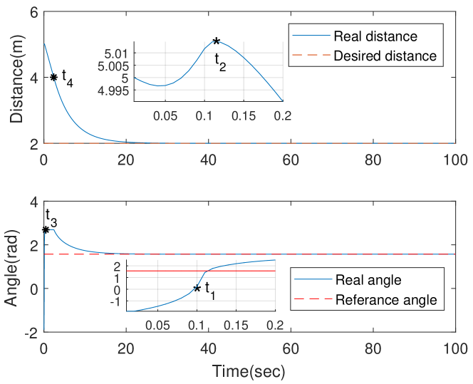
Fig. 4 illustrates the distance d(t)𝑑𝑡d(t) and angle ϕ(t)italic-ϕ𝑡\phi(t) for the initial state 𝒚(t0)=[7,2,3π/5]𝒚subscript𝑡0superscript723𝜋5\bm{y}(t_{0})=[7,2,-3\pi/5]^{\prime}. The dash lines in Fig. 4 represent the desired radius rc=2subscript𝑟𝑐2r_{c}=2 and reference angle π/2𝜋2\pi/2, respectively. It is clear that the target circumnavigation task is eventually completed with zero steady-state error.
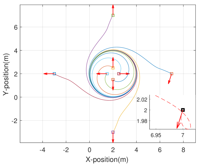
Refer to caption

Figure 3: Trajectories of the robot with different initial states.

Refer to caption

Figure 4: Distance d(t)𝑑𝑡d(t) and angle ϕ(t)italic-ϕ𝑡\phi(t) versus time.

From the partially enlarged view in Fig. 4, we observe that the angle ϕ(t)italic-ϕ𝑡\phi(t) increases from ϕ(t0)=3π/5italic-ϕsubscript𝑡03𝜋5\phi(t_{0})=-3\pi/5 to ϕ(t1)=0italic-ϕsubscript𝑡10\phi(t_{1})=0 at the initial stage. Then, ϕ(t)italic-ϕ𝑡\phi(t) further increases until ϕ(t3)=arccos(k2/vc)italic-ϕsubscript𝑡3subscript𝑘2subscript𝑣𝑐\phi(t_{3})=\arccos(-k_{2}/v_{c}) by crossing ϕ(t2)=π/2italic-ϕsubscript𝑡2𝜋2\phi(t_{2})=\pi/2. From t3subscript𝑡3t_{3} to t4subscript𝑡4t_{4}, ϕ(t)italic-ϕ𝑡\phi(t) maintains the value arccos(k2/vc)subscript𝑘2subscript𝑣𝑐\arccos(-k_{2}/v_{c}), and d(t)𝑑𝑡d(t) converges to rcsubscript𝑟𝑐r_{c} at the speed k2subscript𝑘2-k_{2}. At the time instant t4subscript𝑡4t_{4}, it holds that d(t4)=rc+k3𝑑subscript𝑡4subscript𝑟𝑐subscript𝑘3d(t_{4})=r_{c}+k_{3}. Note that, all these observations are consistent with the statements in Subsection 4.2.
Refer to caption

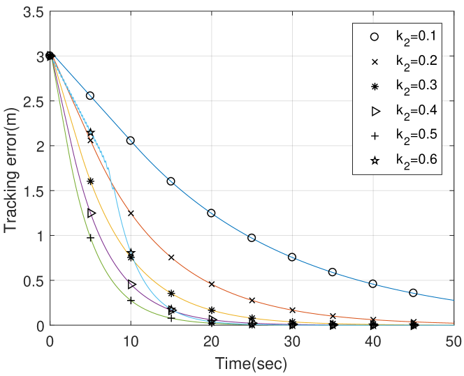
Figure 5: Distance error d(t)rc𝑑𝑡subscript𝑟𝑐d(t)-r_{c} versus time with different k2subscript𝑘2k_{2}.

Fig. 5 shows the relationship between the convergence speed and parameter k2subscript𝑘2k_{2}. The initial state is 𝒚(t0)=[7,2,π/2]𝒚subscript𝑡0superscript72𝜋2\bm{y}(t_{0})=[7,2,-\pi/2]^{\prime}, and the parameters are given in Table 1. If k2>vcsubscript𝑘2subscript𝑣𝑐k_{2}>v_{c}, e.g., k2=0.6subscript𝑘20.6k_{2}=0.6, the oscillation occurs.

6.2 Target encirclement with smooth patterns

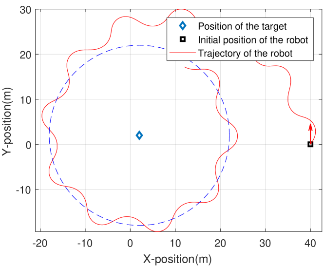
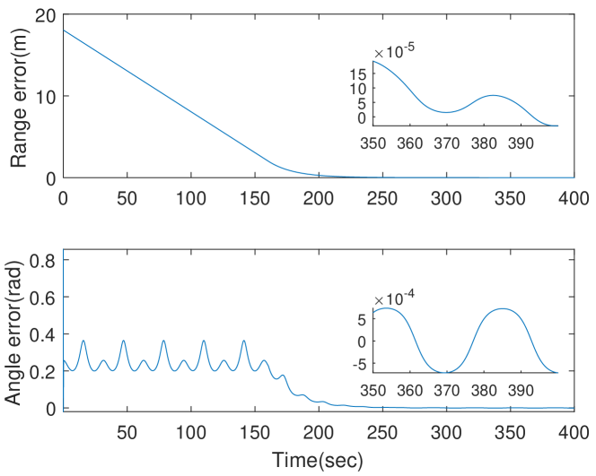
In this subsection, we set the reference command as r(t)=20+1.8sin(0.2t)𝑟𝑡201.80.2𝑡r(t)=20+1.8\sin(0.2t). Obviously, |r˙(t)|rv=0.36˙𝑟𝑡subscript𝑟𝑣0.36|\dot{r}(t)|\leq r_{v}=0.36, and |r¨(t)|ra=0.072¨𝑟𝑡subscript𝑟𝑎0.072|\ddot{r}(t)|\leq r_{a}=0.072. k2subscript𝑘2k_{2} is set as 0.10.10.1 and the other parameters are given in Table 1. Moreover, the initial state is 𝒚(t0)=[40,0,π/2]𝒚subscript𝑡0superscript400𝜋2\bm{y}(t_{0})=[40,0,\pi/2]^{\prime}, satisfying all conditions in Proposition 5.

The results are shown in Fig. 6 and Fig. 7, where the range error is the difference between d(t)𝑑𝑡d(t) and r(t)𝑟𝑡r(t), and the angle error is that between ϕ(t)italic-ϕ𝑡\phi(t) and arccos(r˙(t)/vc)˙𝑟𝑡subscript𝑣𝑐\arccos(\dot{r}(t)/v_{c}). By (3), ϕ(t)=arccos(r˙(t)/vc)italic-ϕ𝑡˙𝑟𝑡subscript𝑣𝑐\phi(t)=\arccos(\dot{r}(t)/v_{c}) implies that d˙(t)=r˙(t)˙𝑑𝑡˙𝑟𝑡\dot{d}(t)=\dot{r}(t). It is clear that 𝒙(t)=[d(t),d˙(t)]𝒙𝑡superscript𝑑𝑡˙𝑑𝑡\bm{x}(t)=[d(t),\dot{d}(t)]^{\prime} converges to 𝒙e(t)=[r(t),r˙(t)]subscript𝒙𝑒𝑡superscript𝑟𝑡˙𝑟𝑡\bm{x}_{e}(t)=[r(t),\dot{r}(t)]^{\prime} as t𝑡t\rightarrow\infty.

Refer to caption

Figure 6: Trajectory of the robot with time-varying commands.

Refer to caption

Figure 7: Distance d(t)𝑑𝑡d(t) and angular ϕ(t)italic-ϕ𝑡\phi(t) versus time with time-varying commands.

6.3 Target encirclement with measurement noises
Refer to caption


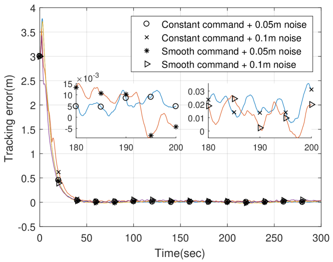
Figure 8: Tracking errors with different level noises.
Table 2: Parameters of the proposed controller
Parameter k1subscript𝑘1k_{1} k2subscript𝑘2k_{2} k3subscript𝑘3k_{3} hh ε1subscript𝜀1\varepsilon_{1} ε2subscript𝜀2\varepsilon_{2}
Value 1 0.25 2.0 1 0.01 0.01

In this subsection, the range measurement is corrupted by an additive white Gaussian noise, i.e.,

d(t)=𝒑(t)𝒑o2+ω(t),𝑑𝑡subscriptnorm𝒑𝑡subscript𝒑𝑜2𝜔𝑡d(t)=\|\bm{p}(t)-\bm{p}_{o}\|_{2}+\omega(t),

where ω(t)𝒩(0,σ2)similar-to𝜔𝑡𝒩0superscript𝜎2\omega(t)\sim\mathcal{N}(0,\sigma^{2}). The constant command and time-varying reference command are set as rc=2subscript𝑟𝑐2r_{c}=2 and r(t)=rc+0.8sin(0.04t)𝑟𝑡subscript𝑟𝑐0.80.04𝑡r(t)=r_{c}+0.8*\sin(0.04t), respectively. Fig. 8 shows the results with different noise level: σ=0.05and0.1𝜎0.05and0.1\sigma=0.05~{}\text{and}~{}0.1, (2.5%rcand5%rcpercent2.5subscript𝑟𝑐andpercent5subscript𝑟𝑐2.5\%r_{c}~{}\text{and}~{}5\%r_{c}). The initial state is 𝒚(t0)=[7,2,π/2]𝒚subscript𝑡072𝜋2\bm{y}(t_{0})=[7,2,-\pi/2], and the parameters are selected as Table 2. From the partially enlarged view of Fig. 8, we observe that the tracking errors are smaller than the measurement errors. This illustrates that the proposed controller is robust against measurement noises.

6.4 Comparison with the existing methods

For comparison, we consider the constraint on control output and let |u(t)|u¯𝑢𝑡¯𝑢|u(t)|\leq\bar{u}, where u¯=1¯𝑢1\bar{u}=1rad/srads\mathrm{r}\mathrm{a}\mathrm{d}\mathrm{/}\mathrm{s} (Matveev et al., 2011) in this subsection. The comparison methods are the geometrical approach (Cao, 2015) with parameters k=1𝑘1k=1 and ra=9.95subscript𝑟𝑎9.95r_{a}=9.95, the switching approach (Zhang et al., 2017) with parameter k=1.4/rc𝑘1.4subscript𝑟𝑐k=1.4/r_{c}, and the sliding mode approach (Matveev et al., 2011) with δ=0.83𝛿0.83\delta=0.83 and γ=0.3𝛾0.3\gamma=0.3.

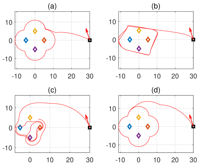
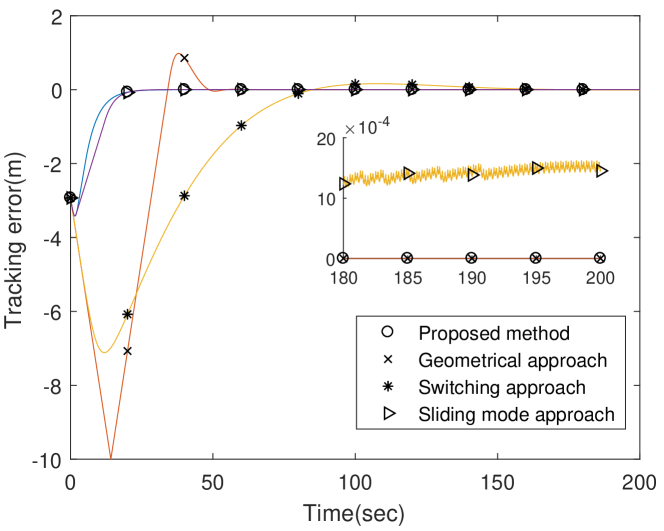
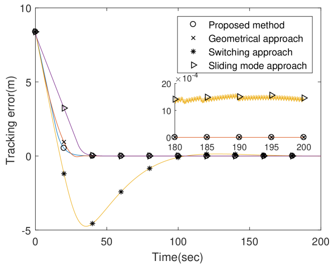
Fig. 9 and Fig. 10 show the results with a constant command rc=10subscript𝑟𝑐10r_{c}=10, where the initial states of the robot are 𝒚(t0)=[7,7,3π/4]𝒚subscript𝑡0773𝜋4\bm{y}(t_{0})=[7,7,-3\pi/4] and 𝒚(t0)=[15,15,3π/4]𝒚subscript𝑡015153𝜋4\bm{y}(t_{0})=[15,15,-3\pi/4], respectively. The parameters are configured as Table 1. When d(t)<ra𝑑𝑡subscript𝑟𝑎d(t)<r_{a}, the control output of the geometrical approach is zero, a large overshoot occurs in this simulation. Furthermore, the convergence speed of the switching approach is slowest. Even though the trajectory generated by the sliding mode approach is similar to that generated by the proposed controller, the sliding mode approach is chattering and has steady-state error, see the partially enlarged view in Fig. 9 and Fig. 10.

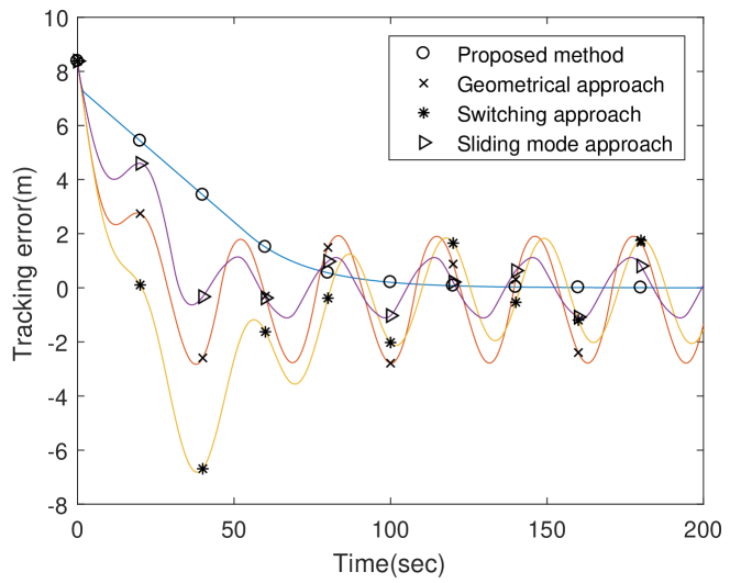
Fig. 11 provides the results with smooth patterns. All the methods in Cao (2015); Zhang et al. (2017); Matveev et al. (2011) fail to follow the time-varying command r(t)=10+1.8sin(0.2t)𝑟𝑡101.80.2𝑡r(t)=10+1.8\sin(0.2t).

To encircle multiple targets as Matveev et al. (2017), let

d(t):=mini𝒑(t)𝒑i2assign𝑑𝑡subscript𝑖subscriptnorm𝒑𝑡subscript𝒑𝑖2d(t):=\min_{i}\|\bm{p}(t)-\bm{p}_{i}\|_{2}

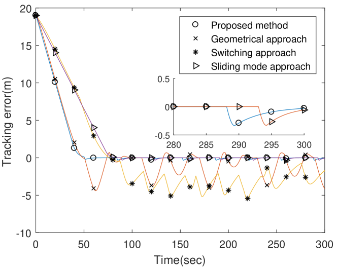
where 𝒑isubscript𝒑𝑖\bm{p}_{i} is the position of the i𝑖i-th target. The trajectories and the tracking errors are given in Fig. 12 and Fig. 13. The proposed method achieves similar performance with that of the sliding mode approach, while either the geometrical approach or the switching approach is unable to complete this task.

Overall, the controller in (4) can handle several target encircling issues, such as measurement noises, time-varying reference commands, and multiple targets in the simulation.
Refer to caption

Figure 9: Comparison of tracking performance with constant reference command.

Refer to caption

Figure 10: Comparison of tracking performance with constant reference command.

Refer to caption

Figure 11: Comparison of tracking performance with time-varying reference command.

Refer to caption

Figure 12: Multi-target encirclement under different control methods: (a) proposed method, (b) geometrical approach, (c) switching approach, (d) sliding mode approach.

Refer to caption

Figure 13: Comparison of tracking performance.

7 Conclusions

In this paper, we have proposed a coordinate-free controller to drive a robot to encircle a stationary target with any smooth patterns by only using the range measurements. The proposed controller, which is inspired by the backstepping control method, can guarantee global convergence and exponential stability with zero steady-state error. The simulations validated our theoretical results.

References

  • (1)
  • Cao (2015) Cao, Y. (2015), ‘UAV circumnavigating an unknown target under a GPS-denied environment with range-only measurements’, Automatica 55, 150–158.
  • Deghat et al. (2014) Deghat, M., Shames, I., Anderson, B. D. O. & Yu, C. (2014), ‘Localization and circumnavigation of a slowly moving target using bearing measurements’, IEEE Transactions on Automatic Control 59(8), 2182–2188.
  • Dobrokhodov et al. (2008) Dobrokhodov, V. N., Kaminer, I. I., Jones, K. D. & Ghabcheloo, R. (2008), ‘Vision-based tracking and motion estimation for moving targets using unmanned air vehicles’, Journal of Guidance Control & Dynamics 31(4), 907–917.
  • Dong & You (2019) Dong, F. & You, K. (2019), Circumnavigation of an unknown target using backstepping control based on range-only measurements, in ‘Chinese Control Conference’.
  • Frew et al. (2007) Frew, E. W., Lawrence, D. A., Dixon, C., Elston, J. & Pisano, W. J. (2007), Lyapunov guidance vector fields for unmanned aircraft applications, in ‘American Control Conference’, pp. 371–376.
  • Frew et al. (2008) Frew, E. W., Lawrence, D. A. & Steve, M. (2008), ‘Coordinated standoff tracking of moving targets using Lyapunov guidance vector fields’, Journal of Guidance Control & Dynamics 31(2), 290–306.
  • Guler & Fidan (2015) Guler, S. & Fidan, B. (2015), Range based target capture and station keeping of nonholonomic vehicles without GPS, in ‘European Control Conference’, pp. 2970–2975.
  • Hafez et al. (2014) Hafez, A. T., Iskandarani, M., Givigi, S. N., Yousefi, S., Rabbath, C. A. & Beaulieu, A. (2014), Using linear model predictive control via feedback linearization for dynamic encirclement, in ‘American Control Conference’, pp. 3868–3873.
  • Hu et al. (2011) Hu, J., Xie, L. & Zhang, C. (2011), ‘Energy-based multiple target localization and pursuit in mobile sensor networks’, IEEE Transactions on Instrumentation & Measurement 61(1), 212–220.
  • Jiang & Nijmeijer (1997) Jiang, Z.-P. & Nijmeijer, H. (1997), ‘Tracking control of mobile robots: A case study in backstepping’, Automatica 33(7), 1393–1399.
  • Khalil (2002) Khalil, H. K. (2002), Nonlinear Systems (3rd Ed.), Prentice Hall.
  • Lawrence (2003) Lawrence, D. (2003), Lyapunov vector fields for UAV flock coordination, in ‘2nd AIAA Unmanned Unlimited Conference, Workshop, and Exhibit’.
  • Lee et al. (2013) Lee, J. K., Park, J. B. & Choi, Y. H. (2013), ‘Tracking control of nonholonomic wheeled mobile robot based on new sliding surface with approach angle’, IFAC Proceedings Volumes 46(29), 38–43.
  • Lin et al. (2016) Lin, J., Song, S., You, K. & Wu, C. (2016), ‘3-D velocity regulation for nonholonomic source seeking without position measurement’, IEEE Transactions on Control Systems Technology 24(2), 711–718.
  • Marasco et al. (2012) Marasco, A. J., Givigi, S. N. & Rabbath, C. A. (2012), Model predictive control for the dynamic encirclement of a target, in ‘American Control Conference’.
  • Matveev et al. (2017) Matveev, A. S., Semakova, A. A. & Savkin, A. V. (2017), ‘Tight circumnavigation of multiple moving targets based on a new method of tracking environmental boundaries’, Automatica 79, 52 – 60.
  • Matveev et al. (2011) Matveev, A. S., Teimoori, H. & Savkin, A. V. (2011), ‘Range-only measurements based target following for wheeled mobile robots’, Automatica 47(1), 177–184.
  • Milutinović et al. (2017) Milutinović, D., Casbeer, D., Cao, Y. & Kingston, D. (2017), ‘Coordinate frame free Dubins vehicle circumnavigation using only range-based measurements’, International Journal of Robust & Nonlinear Control 27(16), 2937–2960.
  • Milutinovic et al. (2014) Milutinovic, D., Casbeer, D., Cao, Y. & Kingston, D. (2014), Coordinate frame free Dubins vehicle circumnavigation, in ‘American Control Conference’, pp. 891–896.
  • Shames et al. (2012) Shames, I., Dasgupta, S., Fidan, B. & Anderson, B. D. O. (2012), ‘Circumnavigation using distance measurements under slow drift’, IEEE Transactions on Automatic Control 57(4), 889–903.
  • Xiao & Lu (2017) Xiao, Y. & Lu, L. (2017), ‘Target enclosing and trajectory tracking for a mobile robot with input disturbances’, IEEE Control Systems Letters 1(2), 221–226.
  • Yu & Liu (2017) Yu, X. & Liu, L. (2017), ‘Target enclosing and trajectory tracking for a mobile robot with input disturbances’, IEEE Control Systems Letters 1(2), 221–226.
  • Zhang & Liu (2010) Zhang, M. & Liu, H. H. T. (2010), Vision-based tracking and estimation of ground moving target using unmanned aerial vehicle, in ‘American Control Conference’, pp. 6968–6973.
  • Zhang et al. (2017) Zhang, M., Tian, P. & Chen, X. (2017), ‘Unmanned aerial vehicle guidance law for ground target circumnavigation using range-based measurements’, International Journal of Control Automation & Systems 15(5), 2455–2460.
  • Zheng et al. (2015) Zheng, R., Liu, Y. & Sun, D. (2015), ‘Enclosing a target by nonholonomic mobile robots with bearing-only measurements’, Automatica 53, 400–407.