On the Noisy Gradient Descent that Generalizes as SGD

Jingfeng Wu    Wenqing Hu    Haoyi Xiong    Jun Huan    Vladimir Braverman    Zhanxing Zhu
Abstract

The gradient noise of SGD is considered to play a central role in the observed strong generalization abilities of deep learning. While past studies confirm that the magnitude and covariance structure of gradient noise are critical for regularization, it remains unclear whether or not the class of noise distributions is important. In this work we provide negative results by showing that noises in classes different from the SGD noise can also effectively regularize gradient descent. Our finding is based on a novel observation on the structure of the SGD noise: it is the multiplication of the gradient matrix and a sampling noise that arises from the mini-batch sampling procedure. Moreover, the sampling noises unify two kinds of gradient regularizing noises that belong to the Gaussian class: the one using (scaled) Fisher as covariance and the one using the gradient covariance of SGD as covariance. Finally, thanks to the flexibility of choosing noise class, an algorithm is proposed to perform noisy gradient descent that generalizes well, the variant of which even benefits large batch SGD training without hurting generalization.

SGD, Noise, Regularization

1 Introduction

Stochastic gradient descent (SGD) is one of the standard workhorses for optimizing deep models (Bottou, 1991). Though initially proposed to remedy the computational bottleneck of gradient descent (GD), recent studies suggest SGD in addition induces a crucial implicit regularization, which prevents the over-parameterized models from converging to the minima that cannot generalize well (Zhang et al., 2017; Zhu et al., 2018; Jastrzębski et al., 2017; Hoffer et al., 2017; Keskar et al., 2017). To gain intuitions, one can compare the generalization abilities of (i) GD vs. SGD, (ii) small batch SGD vs. large batch SGD, and (iii) SGD vs. gradient Langevin dynamic (GLD). Empirical studies confirm that (i) SGD outperforms GD (Zhu et al., 2018), (ii) small batch SGD generalizes better than large batch SGD (Hoffer et al., 2017; Keskar et al., 2017), and (iii) GLD cannot compete with SGD (Zhu et al., 2018). To understand why these phenomena happen, let us look at the differences between the compared algorithms. Firstly SGD can be viewed as GD, an deterministic algorithm, with an unbiased noise inserted at every iteration, which is called the gradient noise (Bottou et al., 2018). Secondly the gradient noise of the small batch SGD has a much larger magnitude than that of the large batch SGD (Hoffer et al., 2017; Jastrzębski et al., 2017). Thirdly, even though the noise magnitude is tuned to be equal, the SGD noise has a nontrivial covariance structure, instead of just being a white noise as in GLD (Zhu et al., 2018). The above discussions exhibit a critical fact:

Certain noises can effectively regularize gradient descent.

Despite the efforts spent, this important yet implicit regularization effect induced by noise has never been fully understood. From the Bayesian perspective, the noise is interpreted to perform variational inference (Mandt et al., 2017; Chaudhari & Soatto, 2017). Such interpretation, however, requires unrealistic assumptions such as the noise has constant covariance (Mandt et al., 2017) or certain force is conservative (Chaudhari & Soatto, 2017). Another theory argues that the noise enables the gradient algorithm to escape from sharp minima (Zhu et al., 2018; Hu et al., 2019; Simsekli et al., 2019) that typically generalize worse (Hochreiter & Schmidhuber, 1997; Keskar et al., 2017). Hence GD enhanced by such noise tends to find flat minima that generalize well. This explanation hold valid to some extent; but the escaping behavior is too subtle to fit practice — the loss/accuracy does not jump significantly after the dynamic reaching a minimum, e.g., see the final epochs of Figure 4 in (Huang et al., 2017). Therefore the algorithm does not explicitly escape from minima in practice. Although the mechanism has not been completely understood, we can still recognize and utilize such implicit regularization by studying the properties of gradient noise.

We next summarize three important aspects of gradient noise that might introduce the regularization effects: noise magnitude, covariance structure and distribution class of noise.

Noise magnitude  The large batch SGD encounters performance deterioration compared with the small batch one, thus the magnitude of gradient noise matters (Hoffer et al., 2017; Keskar et al., 2017; Smith & Le, 2018). Furthermore, Jastrzębski et al. (2017) show that the ratio of learning rate to batch size, which directly controls the noise magnitude, has an important influence on the generalization of SGD: in a certain range, greater the ratio, larger the noise, and better the generalization.

Noise covariance structure  From the perspective of escaping from minima, Zhu et al. (2018) emphasize the importance of the noise covariance structure for regularization. They show that when the noise covariance contains curvature information, it performs better for escaping from sharp minima (Zhu et al., 2018; Hu et al., 2019; Daneshmand et al., 2018). Surprisingly, the covariance of the SGD noise aligns with the Hessian of the loss surface to some extent (Zhu et al., 2018; Li et al., 2019), which then partly explains the benefits brought by the SGD noise.

Noise class  Many works assume that the SGD noise belongs to the Gaussian class due to the classical central limit theorem  (Ahn et al., 2012; Chen et al., 2014; Shang et al., 2015; Mandt et al., 2017; Zhu et al., 2018). Nonetheless, Simsekli et al. (2019) first argue that the second moment of SGD noise might not exist, thus the Gaussianity assumption requires a second thought, since the classical central limit theorem has to be revised for heavy-tailed distributions (Gnedenko & Kolmogorov, 1968; Bertoin, 1998). Instead in this case, the central limit theorem leads to Levy distribution which they adopt for modeling SGD noise. By assuming so they obtain a faster escaping behavior of SGD (Simsekli et al., 2019; Nguyen et al., 2019; Şimşekli et al., 2019). Later Panigrahi et al. (2019) directly perform Gasussianity testing during the process of SGD learning deep neural networks. They empirically find that when the batch size is greater than 256256256, the SGD noise can be treated as Gaussian in the early phase of training; but in general the SGD noise does not have to be Gaussian alike.

While past studies confirm the importance of noise magnitude and covariance structure, the role of noise class in regularizing a gradient method has not been fully explored. In this work, we attempt to address this issue from a novel perspective of sampling noise. Taking SGD for instance, we notice the gradient noise is indeed caused by the mini-batch sampling procedure. This observation enables us to establish a key notion called the sampling noise to characterize the stochasticity of mini-batch sampling. Based on the sampling noise, we show that noises in classes different from the SGD noise can also effectively regularize gradient descent, thus provide negative evidence on the impact of the noise class. On the other hand, thanks to the flexibility of choosing noise class, we are allowed to use noisy gradient descent with best fitted noises based on practical requirements, beyond the vanilla SGD. This finding supports the methods to employ structured Gaussian noises for improving GD/large batch SGD (Zhu et al., 2018; Wen et al., 2019).

Contributions  In summary we obtain the following important results:

  1. 1.

    A novel perspective is proposed for interpreting the SGD noise: it is the multiplication of a gradient matrix and a sampling noise which raises from the mini-batch sampling process. A general class of noisy gradient descent is thus defined based on the sampling noise.

  2. 2.

    The regularization role of the distribution class of gradient noise is then investigated. In both theory and experiments, we demonstrate that the noise class might not be a crux for regularization, provided suitable noise magnitude and covariance structure.

  3. 3.

    Two kinds of gradient regularizing noises from the Gaussian classes are then revised, i.e., the one using the (scaled) Fisher as covariance (Wen et al., 2019) and the one employing the gradient covariance of SGD as covariance (Zhu et al., 2018). The equivalence between them is established by analyzing their sampling noises.

  4. 4.

    Thanks to the unimportance of the noise class, an algorithm is proposed to perform generalizable noisy gradient descent with noises from various classes. Its variant even benefits large batch SGD training without hurting generalization.

2 The gradient noise of SGD

Let the training data be {xi}i=1nsuperscriptsubscriptsubscript𝑥𝑖𝑖1𝑛\{x_{i}\}_{i=1}^{n}, and consider the empirical loss L(θ)=1ni=1n(xi;θ)𝐿𝜃1𝑛superscriptsubscript𝑖1𝑛subscript𝑥𝑖𝜃L(\theta)=\frac{1}{n}\sum_{i=1}^{n}\ell(x_{i};\theta), where (x;θ)𝑥𝜃\ell(x;\theta) is the loss over one sample and θd𝜃superscript𝑑\theta\in\mathbbm{R}^{d} is the parameter to be optimized. Define the loss vector as (θ)=((x1;θ),,(xn;θ))1×n𝜃subscript𝑥1𝜃subscript𝑥𝑛𝜃superscript1𝑛\mathcal{L}(\theta)=\left(\ell(x_{1};\theta),\dots,\ell(x_{n};\theta)\right)\in\mathbbm{R}^{1\times n}, then the gradient matrix is θ(θ)=(θ(x1;θ),,θ(xn;θ))d×nsubscript𝜃𝜃subscript𝜃subscript𝑥1𝜃subscript𝜃subscript𝑥𝑛𝜃superscript𝑑𝑛\operatorname{\nabla}_{\theta}\mathcal{L}(\theta)=\left(\operatorname{\nabla}_{\theta}\ell(x_{1};\theta),\dots,\operatorname{\nabla}_{\theta}\ell(x_{n};\theta)\right)\in\mathbbm{R}^{d\times n}. Let 𝟙=(1,,1)Tn1superscript11𝑇superscript𝑛\mathbbm{1}=(1,\dots,1)^{T}\in\mathbbm{R}^{n}, then L(θ)=1n(θ)𝟙𝐿𝜃1𝑛𝜃1L(\theta)=\frac{1}{n}\mathcal{L}(\theta)\cdot\mathbbm{1}.

SGD  During each iteration of SGD, the algorithm first randomly draws a mini-batch of samples with index set Bt={i1,,ib}subscript𝐵𝑡subscript𝑖1subscript𝑖𝑏B_{t}=\{i_{1},\dots,i_{b}\} in size |Bt|=bsubscript𝐵𝑡𝑏|B_{t}|=b, and then performs parameter update using the stochastic gradient g~(θ)~𝑔𝜃\tilde{g}(\theta) computed by the mini-batch and learning rate η𝜂\eta,

θt+1=θtηg~(θt),g~(θt)=1biBtθ(xi;θt).formulae-sequencesubscript𝜃𝑡1subscript𝜃𝑡𝜂~𝑔subscript𝜃𝑡~𝑔subscript𝜃𝑡1𝑏subscript𝑖subscript𝐵𝑡subscript𝜃subscript𝑥𝑖subscript𝜃𝑡\theta_{t+1}=\theta_{t}-\eta\tilde{g}(\theta_{t}),\quad\tilde{g}(\theta_{t})=\frac{1}{b}\sum_{i\in B_{t}}\operatorname{\nabla}_{\theta}\ell(x_{i};\theta_{t}).

Sampling noise  Note that the stochasticity of g~(θt)~𝑔subscript𝜃𝑡\tilde{g}(\theta_{t}) is caused by the randomness of the mini-batch sampling procedure, thus the stochastic gradient could be written as

g~(θt)=θ(θt)𝒲sgd,~𝑔subscript𝜃𝑡subscript𝜃subscript𝜃𝑡subscript𝒲sgd\tilde{g}(\theta_{t})=\operatorname{\nabla}_{\theta}\mathcal{L}(\theta_{t})\cdot\mathcal{W}_{\mathrm{sgd}},

where 𝒲sgdnsubscript𝒲sgdsuperscript𝑛\mathcal{W}_{\mathrm{sgd}}\in\mathbbm{R}^{n} is a random sampling vector characterizing the mini-batch sampling process. For instance considering mini-batch SGD without replacement, the sampling vector 𝒲sgdsubscript𝒲sgd\mathcal{W}_{\mathrm{sgd}} contains exactly b𝑏b multiples of 1b1𝑏\frac{1}{b} and nb𝑛𝑏n-b multiples of zero with random index. It is easy to see that 𝔼[𝒲sgd]=1n𝟙𝔼delimited-[]subscript𝒲sgd1𝑛1\mathbbm{E}[\mathcal{W}_{\mathrm{sgd}}]=\frac{1}{n}\mathbbm{1}, thus 𝔼[g~(θt)]=1nθ(θt)𝟙=θL(θt)𝔼delimited-[]~𝑔subscript𝜃𝑡1𝑛subscript𝜃subscript𝜃𝑡1subscript𝜃𝐿subscript𝜃𝑡\mathbbm{E}[\tilde{g}(\theta_{t})]=\frac{1}{n}\operatorname{\nabla}_{\theta}\mathcal{L}(\theta_{t})\cdot\mathbbm{1}=\operatorname{\nabla}_{\theta}L(\theta_{t}), i.e., the stochastic gradient g~(θt)~𝑔subscript𝜃𝑡\tilde{g}(\theta_{t}) is an unbiased estimator of the full gradient θL(θt)subscript𝜃𝐿subscript𝜃𝑡\operatorname{\nabla}_{\theta}L(\theta_{t}).

Define the sampling noise as 𝒱sgd=𝒲sgd1n𝟙subscript𝒱sgdsubscript𝒲sgd1𝑛1\mathcal{V}_{\mathrm{sgd}}=\mathcal{W}_{\mathrm{sgd}}-\frac{1}{n}\mathbbm{1}. Then the stochastic gradient has the decomposition of

g~(θt)=θL(θt)+θ(θt)𝒱sgd,𝔼[𝒱sgd]=0.formulae-sequence~𝑔subscript𝜃𝑡subscript𝜃𝐿subscript𝜃𝑡subscript𝜃subscript𝜃𝑡subscript𝒱sgd𝔼delimited-[]subscript𝒱sgd0\tilde{g}(\theta_{t})=\operatorname{\nabla}_{\theta}L(\theta_{t})+\operatorname{\nabla}_{\theta}\mathcal{L}(\theta_{t})\cdot\mathcal{V}_{\mathrm{sgd}},\quad\mathbbm{E}[\mathcal{V}_{\mathrm{sgd}}]=0.

The first two moments of 𝒱sgdsubscript𝒱sgd\mathcal{V}_{\mathrm{sgd}} are given in Proposition 1.

Proposition 1.

(Mean and covariance of the SGD sampling noise) For mini-batch sampled without replacement, the SGD sampling noise 𝒱sgdsubscript𝒱sgd\mathcal{V}_{\mathrm{sgd}} satisfies

𝔼[𝒱sgd]=0,Var[𝒱sgd]=nbbn(n1)(I1n𝟙𝟙T).formulae-sequence𝔼delimited-[]subscript𝒱sgd0Varsubscript𝒱sgd𝑛𝑏𝑏𝑛𝑛1𝐼1𝑛superscript11𝑇\mathbbm{E}[\mathcal{V}_{\mathrm{sgd}}]=0,\quad\operatorname{Var}[\mathcal{V}_{\mathrm{sgd}}]=\frac{n-b}{bn(n-1)}\left(I-\frac{1}{n}\mathbbm{1}\mathbbm{1}^{T}\right).

For mini-batch sampled with replacement, the SGD sampling noise 𝒱sgdsuperscriptsubscript𝒱sgd\mathcal{V}_{\mathrm{sgd}}^{\prime} satisfies

𝔼[𝒱sgd]=0,Var[𝒱sgd]=1bn(I1n𝟙𝟙T).formulae-sequence𝔼delimited-[]superscriptsubscript𝒱sgd0Varsuperscriptsubscript𝒱sgd1𝑏𝑛𝐼1𝑛superscript11𝑇\mathbbm{E}[\mathcal{V}_{\mathrm{sgd}}^{\prime}]=0,\quad\operatorname{Var}[\mathcal{V}_{\mathrm{sgd}}^{\prime}]=\frac{1}{bn}\left(I-\frac{1}{n}\mathbbm{1}\mathbbm{1}^{T}\right).

The proof is left in Section A.1 of the Supplementary Materials. If not stated otherwise, we focus on SGD with replacement in the remaining parts. However, our arguments hold for both of them with mild modifications.

Gradient noise  From the viewpoint of sampling noise, the gradient noise of SGD is the multiplication of the gradient matrix and its sampling noise,

υsgd(θt)=g~(θt)θL(θt)=θ(θt)𝒱sgd.subscript𝜐sgdsubscript𝜃𝑡~𝑔subscript𝜃𝑡subscript𝜃𝐿subscript𝜃𝑡subscript𝜃subscript𝜃𝑡subscript𝒱sgd\upsilon_{\mathrm{sgd}}(\theta_{t})=\tilde{g}(\theta_{t})-\operatorname{\nabla}_{\theta}L(\theta_{t})=\operatorname{\nabla}_{\theta}\mathcal{L}(\theta_{t})\cdot\mathcal{V}_{\mathrm{sgd}}.

Note that while the sampling noise 𝒱sgdsubscript𝒱sgd\mathcal{V}_{\mathrm{sgd}} is state-independent, the gradient noise υsgd(θt)subscript𝜐sgdsubscript𝜃𝑡\upsilon_{\mathrm{sgd}}(\theta_{t}) is coupled with the parameter θtsubscript𝜃𝑡\theta_{t}. By Proposition 1, the first two moments of the gradient noise are 𝔼[υsgd(θt)]=θ(θt)𝔼[𝒱sgd]=0𝔼delimited-[]subscript𝜐sgdsubscript𝜃𝑡subscript𝜃subscript𝜃𝑡𝔼delimited-[]subscript𝒱sgd0\mathbbm{E}[\upsilon_{\mathrm{sgd}}(\theta_{t})]=\operatorname{\nabla}_{\theta}\mathcal{L}(\theta_{t})\mathbbm{E}[\mathcal{V}_{\mathrm{sgd}}]=0 and

C(θt)=Var[υsgd(θt)]=θ(θt)Var[𝒱sgd]θ(θt)T𝐶subscript𝜃𝑡Varsubscript𝜐sgdsubscript𝜃𝑡subscript𝜃subscript𝜃𝑡Varsubscript𝒱sgdsubscript𝜃superscriptsubscript𝜃𝑡𝑇\displaystyle C(\theta_{t})=\operatorname{Var}[\upsilon_{\mathrm{sgd}}(\theta_{t})]=\operatorname{\nabla}_{\theta}\mathcal{L}(\theta_{t})\operatorname{Var}[\mathcal{V}_{\mathrm{sgd}}]\operatorname{\nabla}_{\theta}\mathcal{L}(\theta_{t})^{T} (1)
=1b(1n(θt)(θt)TL(θt)L(θt)T).absent1𝑏1𝑛subscript𝜃𝑡superscriptsubscript𝜃𝑡𝑇𝐿subscript𝜃𝑡𝐿superscriptsubscript𝜃𝑡𝑇\displaystyle=\frac{1}{b}\left(\frac{1}{n}\operatorname{\nabla}\mathcal{L}(\theta_{t})\operatorname{\nabla}\mathcal{L}(\theta_{t})^{T}-\operatorname{\nabla}L(\theta_{t})\operatorname{\nabla}L(\theta_{t})^{T}\right).

In the following we call C(θt)𝐶subscript𝜃𝑡C(\theta_{t}) the SGD covariance.

As the structure of the SGD noise is clear, we turn to discuss the properties of the noise that affect its implicit regularization. Studies on large batch SGD training (Keskar et al., 2017; Hoffer et al., 2017) exhibit the importance of the noise magnitude, which is controlled by ηb𝜂𝑏\sqrt{\tfrac{\eta}{b}} (Jastrzębski et al., 2017). And from the viewpoint of escaping from minima, the implicit bias of SGD is also closely related to the noise covariance structure C(θ)𝐶𝜃C(\theta)  (Zhu et al., 2018; Hu et al., 2019; Li et al., 2019). Recently, the role of the noise class raises research interests, as discussed below.

2.1 The class of the SGD noise

Due to the i.i.d. sampling of a mini-batch, as the batch size approaches infinity, the theory about limit theorems guarantees that the SGD noise converges to certain infinite divisible distribution (Gnedenko & Kolmogorov, 1968; Bertoin, 1998). If the second moment of the noise is finite, the limiting infinite divisible distribution will belong to the Gaussian class. Thus many works assume the Gaussianity of the SGD noise (Chen et al., 2014; Ahn et al., 2012; Shang et al., 2015; Mandt et al., 2017; Jastrzębski et al., 2017; Zhu et al., 2018). However, if the second moment does not exist, so that the noise is heavy-tailed, then the gradient noise should converge to a Levy type distribution, as assumed by (Simsekli et al., 2019; Nguyen et al., 2019; Şimşekli et al., 2019). Moreover, it is also questionable whether in practice the batch size is large enough for applying limit theorems. We investigate the two issues in the following.

The finiteness of the SGD covariance  Based on analysis of the structure of the SGD noise, we have C(θt)=θ(θt)Var[𝒱sgd]θ(θt)T𝐶subscript𝜃𝑡subscript𝜃subscript𝜃𝑡Varsubscript𝒱sgdsubscript𝜃superscriptsubscript𝜃𝑡𝑇C(\theta_{t})=\operatorname{\nabla}_{\theta}\mathcal{L}(\theta_{t})\operatorname{Var}[\mathcal{V}_{\mathrm{sgd}}]\operatorname{\nabla}_{\theta}\mathcal{L}(\theta_{t})^{T} by Eq. (1), and Var[𝒱sgd]Varsubscript𝒱sgd\operatorname{Var}[\mathcal{V}_{\mathrm{sgd}}] is finite by Proposition 1. Thus if the gradient matrix θ(θt)subscript𝜃subscript𝜃𝑡\operatorname{\nabla}_{\theta}\mathcal{L}(\theta_{t}) is bounded (almost everywhere), then C(θt)𝐶subscript𝜃𝑡C(\theta_{t}) must be finite (almost everywhere). Firstly, the typical components of neural networks are twice differentiable (almost everywhere) (Goodfellow et al., 2016); moreover, with common deep learning tricks such as near-zero initialization, early stopping, learning rate decay, weight decay, etc, the optimization process only happens in a small area around the near-zero initialization (Neyshabur et al., 2017; Jacot et al., 2018; Cao & Gu, 2019). Therefore it is reasonable to assume that the gradient matrix θ(θt)subscript𝜃subscript𝜃𝑡\operatorname{\nabla}_{\theta}\mathcal{L}(\theta_{t}) is bounded almost everywhere in the area of our concerns. Thereby we argue that it is safe to assume the finiteness of the SGD covariance.

The non-Gaussianity of the SGD noise  Even with finite covariance, it is still unclear whether in practice the batch size is sufficiently large for the Gaussian to be a good approximation for the SGD noise, especially when it comes to the extremely high dimensional parameter in deep learning. To validate this, Panigrahi et al. (2019) directly perform Gaussianity tests to the SGD noise during the training of deep neural networks. They empirically find that when the batch size is greater than 256256256, the SGD noise behaves like a Gaussian one in the early phase of training; but generally the SGD noise does not belong to the Gaussian class.

The impact of the noise class  We conclude that the SGD noise belongs to a particular distribution class that is neither Levy nor Gaussian. One might wonder if this particular distribution class of SGD noise is crucial for its regularization effects. In the remaining of this work, we address this issue by studying a general framework of noisy gradient descent which can employ noises from various classes, including the SGD noise class and the Gaussian class. The framework is called the multiplicative SGD (MSGD).

2.2 Multiplicative SGD

During each iteration, the proposed MSGD randomly generates a sampling vector 𝒲n𝒲superscript𝑛\mathcal{W}\in\mathbbm{R}^{n} with mean as 𝔼[𝒲]=1n𝟙𝔼delimited-[]𝒲1𝑛1\mathbbm{E}[\mathcal{W}]=\frac{1}{n}\mathbbm{1}, and then takes update

θt+1=θtηθ(θt)𝒲.subscript𝜃𝑡1subscript𝜃𝑡𝜂subscript𝜃subscript𝜃𝑡𝒲\theta_{t+1}=\theta_{t}-\eta\operatorname{\nabla}_{\theta}\mathcal{L}(\theta_{t})\mathcal{W}.

Denote the sampling noise as 𝒱=𝒲1N𝟙𝒱𝒲1𝑁1\mathcal{V}=\mathcal{W}-\frac{1}{N}\mathbbm{1}, then the gradient noise is υ(θt)=θ(θt)𝒱𝜐subscript𝜃𝑡subscript𝜃subscript𝜃𝑡𝒱\upsilon(\theta_{t})=\operatorname{\nabla}_{\theta}\mathcal{L}(\theta_{t})\mathcal{V}. Since our goal is to study the impact of noise class, the covariance of the gradient noise thus has to be fixed for excluding the influences of the noise magnitude and covariance structure. To this end it is sufficient to fix the covariance of the sampling noise, i.e., Var[𝒱]=Var[𝒱sgd]Var𝒱Varsubscript𝒱sgd\operatorname{Var}[\mathcal{V}]=\operatorname{Var}[\mathcal{V}_{\mathrm{sgd}}]. The MSGD can then be written as

θt+1=θtηθL(θt)+ηθ(θt)𝒱,subscript𝜃𝑡1subscript𝜃𝑡𝜂subscript𝜃𝐿subscript𝜃𝑡𝜂subscript𝜃subscript𝜃𝑡𝒱\displaystyle\theta_{t+1}=\theta_{t}-\eta\operatorname{\nabla}_{\theta}L(\theta_{t})+\eta\operatorname{\nabla}_{\theta}\mathcal{L}(\theta_{t})\mathcal{V}, (2)
where𝔼[𝒱]=0,Var[𝒱]=Var[𝒱sgd].formulae-sequencewhere𝔼delimited-[]𝒱0Var𝒱Varsubscript𝒱sgd\displaystyle\text{where}\quad\mathbbm{E}[\mathcal{V}]=0,\quad\operatorname{Var}[\mathcal{V}]=\operatorname{Var}[\mathcal{V}_{\mathrm{sgd}}].

In the MSGD iteration (2), the gradient noise υ(θt)𝜐subscript𝜃𝑡\upsilon(\theta_{t}) is decided by the deterministic gradient matrix θ(θt)subscript𝜃subscript𝜃𝑡\operatorname{\nabla}_{\theta}\mathcal{L}(\theta_{t}) and a sampling noise 𝒱𝒱\mathcal{V}. Thus we can control the class of the gradient noise by choosing the class of the sampling noise. For example, the gradient noise υ(θt)𝜐subscript𝜃𝑡\upsilon(\theta_{t}) becomes the SGD noise if 𝒱=𝒱sgd𝒱subscript𝒱sgd\mathcal{V}=\mathcal{V}_{\mathrm{sgd}}. Besides, if the sampling noise belongs to the Gaussian class, i.e., 𝒱G𝒩(0,Var[𝒱sgd])similar-tosubscript𝒱G𝒩0Varsubscript𝒱sgd\mathcal{V}_{\text{G}}\sim\mathcal{N}\left(0,\operatorname{Var}[\mathcal{V}_{\mathrm{sgd}}]\right), then the gradient noise υG(θt)=θ(θt)𝒱Gsubscript𝜐Gsubscript𝜃𝑡subscript𝜃subscript𝜃𝑡subscript𝒱G\upsilon_{\text{G}}(\theta_{t})=\operatorname{\nabla}_{\theta}\mathcal{L}(\theta_{t})\mathcal{V}_{\text{G}} is also Gaussian, i.e., υG(θt)𝒩(0,C(θt))similar-tosubscript𝜐Gsubscript𝜃𝑡𝒩0𝐶subscript𝜃𝑡\upsilon_{\text{G}}(\theta_{t})\sim\mathcal{N}\left(0,C(\theta_{t})\right), where C(θt)=θ(θt)Var[𝒱sgd]θ(θt)T𝐶subscript𝜃𝑡subscript𝜃subscript𝜃𝑡Varsubscript𝒱sgdsubscript𝜃superscriptsubscript𝜃𝑡𝑇C(\theta_{t})=\operatorname{\nabla}_{\theta}\mathcal{L}(\theta_{t})\operatorname{Var}[\mathcal{V}_{\mathrm{sgd}}]\operatorname{\nabla}_{\theta}\mathcal{L}(\theta_{t})^{T} by Eq. (1). In this case we call the iteration (2) the Gaussian MSGD. Moreover, gradient noises in other classes of practical interests can also be obtained with suitable sampling noises, e.g., Bernoulli sampling noises and sparse Gaussian sampling noises.

We then explore the role of the noise class by studying the generalization abilities of the MSGD iteration (2) with noises from different classes.

3 Theoretical study

We first theoretically revise the role of the noise class for regularizing the algorithm. For the solution θ^^𝜃\hat{\theta} found by noisy gradient descent and the optimal parameter θsubscript𝜃\theta_{*}, the generalization error can be measured as 𝔼x,θ^[(x;θ^)(x;θ)]subscript𝔼𝑥^𝜃delimited-[]𝑥^𝜃𝑥subscript𝜃\mathbbm{E}_{x,\hat{\theta}}\left[\ell(x;\hat{\theta})-\ell(x;\theta_{*})\right]. Now suppose the loss function (x;θ)𝑥𝜃\ell(x;\theta) can be approximated by a quadratic one (with respect to θ𝜃\theta), then the generalization error involves just the first two moments of θ^^𝜃\hat{\theta}, which depends on at most the second moment information about the gradient noise, since the noise only accumulates linearly in the final solution θ^^𝜃\hat{\theta} because of the linearity of the gradient. Hence intuitively, provided the noise covariance, the generalization error has little dependence on the particular class that the gradient noise belongs to.

To formalize the above intuition, we follow the setting of (Bach & Moulines, 2013; Dieuleveut et al., 2017; Défossez & Bach, 2015) and consider an online linear regression problem

minθf(θ):=12𝔼(x,y)[(xTθy)2].assignsubscript𝜃𝑓𝜃12subscript𝔼𝑥𝑦delimited-[]superscriptsuperscript𝑥𝑇𝜃𝑦2\min_{\theta}f(\theta):=\frac{1}{2}\mathbbm{E}_{(x,y)}[(x^{T}\theta-y)^{2}]. (𝒫𝒫\mathcal{P})

Let Σ=𝔼x[xxT]Σsubscript𝔼𝑥delimited-[]𝑥superscript𝑥𝑇\Sigma=\mathbbm{E}_{x}[xx^{T}], then f(θ)𝑓𝜃f(\theta) always admits an optimal θ=Σ𝔼(x,y)[yx]subscript𝜃superscriptΣsubscript𝔼𝑥𝑦delimited-[]𝑦𝑥\theta_{*}=\Sigma^{\dagger}\mathbbm{E}_{(x,y)}[yx]. Denote the residual as ϵ=yxTθitalic-ϵ𝑦superscript𝑥𝑇subscript𝜃\epsilon=y-x^{T}\theta_{*}, then 𝔼[ϵx]=0𝔼delimited-[]italic-ϵ𝑥0\mathbbm{E}[\epsilon x]=0. We also adopt the following standard assumptions (Bach & Moulines, 2013; Dieuleveut et al., 2017; Défossez & Bach, 2015):

𝔼[x22xxT]R2Σ;precedes-or-equals𝔼delimited-[]superscriptsubscriptnorm𝑥22𝑥superscript𝑥𝑇superscript𝑅2Σ\displaystyle\mathbbm{E}\left[\left\|x\right\|_{2}^{2}xx^{T}\right]\preceq R^{2}\Sigma; (𝒜1subscript𝒜1\mathcal{A}_{1})
𝔼[ϵ2xxT]σ2Σ;precedes-or-equals𝔼delimited-[]superscriptitalic-ϵ2𝑥superscript𝑥𝑇superscript𝜎2Σ\displaystyle\mathbbm{E}\left[\epsilon^{2}xx^{T}\right]\preceq\sigma^{2}\Sigma; (𝒜2subscript𝒜2\mathcal{A}_{2})
ΣλI.precedes-or-equalsΣ𝜆𝐼\displaystyle\Sigma\preceq\lambda I. (𝒜3subscript𝒜3\mathcal{A}_{3})
Remark.

The assumption (𝒜1subscript𝒜1\mathcal{A}_{1}) is satisfied when the data is almost surely bounded, i.e., x2Rsubscriptnorm𝑥2𝑅\left\|x\right\|_{2}\leq R; and (𝒜2subscript𝒜2\mathcal{A}_{2}) holds for almost surely bounded data or when the model is well-specified, i.e., ϵnsubscriptitalic-ϵ𝑛\epsilon_{n} is independent with xnsubscript𝑥𝑛x_{n}, and i.i.d. of zero mean and variance σ2superscript𝜎2\sigma^{2} (Dieuleveut et al., 2017).

Typically the problem (𝒫𝒫\mathcal{P}) is learned by the averaged solution θ¯n=1n+1i=0nθisubscript¯𝜃𝑛1𝑛1superscriptsubscript𝑖0𝑛subscript𝜃𝑖\bar{\theta}_{n}=\frac{1}{n+1}\sum_{i=0}^{n}\theta_{i} of the (small batch) SGD (Bach & Moulines, 2013; Dieuleveut et al., 2017; Défossez & Bach, 2015)

θn+1=θnηrbn(xrxrTθnyrxr),subscript𝜃𝑛1subscript𝜃𝑛𝜂subscript𝑟subscript𝑏𝑛subscript𝑥𝑟superscriptsubscript𝑥𝑟𝑇subscript𝜃𝑛subscript𝑦𝑟subscript𝑥𝑟\theta_{n+1}=\theta_{n}-\eta\sum_{r\in b_{n}}\left(x_{r}x_{r}^{T}\theta_{n}-y_{r}x_{r}\right), (3)

where bnsubscript𝑏𝑛b_{n} is the index set of a randomly sampled mini-batch with a small batch size |bn|=bsubscript𝑏𝑛𝑏|b_{n}|=b. We note b𝑏b could be 111. To validate our understanding, we also consider the following (large batch) MSGD algorithm

θn+1=θnηrBnwr(xrxrTθnyrxr),subscript𝜃𝑛1subscript𝜃𝑛𝜂subscript𝑟subscript𝐵𝑛subscript𝑤𝑟subscript𝑥𝑟superscriptsubscript𝑥𝑟𝑇subscript𝜃𝑛subscript𝑦𝑟subscript𝑥𝑟\theta_{n+1}=\theta_{n}-\eta\sum_{r\in B_{n}}w_{r}\left(x_{r}x_{r}^{T}\theta_{n}-y_{r}x_{r}\right), (4)

where Bnsubscript𝐵𝑛B_{n} is the index set of a randomly sampled mini-batch, with a relatively large batch size |Bn|=B>bsubscript𝐵𝑛𝐵𝑏|B_{n}|=B>b, and 𝒲=(wr1,,wrB)T𝒲superscriptsubscript𝑤subscript𝑟1subscript𝑤subscript𝑟𝐵𝑇\mathcal{W}=(w_{r_{1}},\dots,w_{r_{B}})^{T} is a random sampling vector where 𝔼[𝒲]=1B𝟙𝔼delimited-[]𝒲1𝐵1\mathbbm{E}[\mathcal{W}]=\frac{1}{B}\mathbbm{1}.

The following theorem characterizes the generalization error of the large batch MSGD (4) and the small batch SGD (3).

Theorem 1.

Suppose the covariance of the sampling vector in MSGD (4) satisfies Var[𝒲]=BbbB(B1)(I1B𝟙𝟙T)Var𝒲𝐵𝑏𝑏𝐵𝐵1𝐼1𝐵superscript11𝑇\operatorname{Var}[\mathcal{W}]=\frac{B-b}{bB(B-1)}\left(I-\frac{1}{B}\mathbbm{1}\mathbbm{1}^{T}\right). Then for both of the large batch MSGD (4) and the small batch SGD (3), we have

𝔼θ¯n[f(θ¯n)]f(θ)C1n+1+C2(n+1)2,subscript𝔼subscript¯𝜃𝑛delimited-[]𝑓subscript¯𝜃𝑛𝑓subscript𝜃subscript𝐶1𝑛1subscript𝐶2superscript𝑛12\mathbbm{E}_{\bar{\theta}_{n}}[f(\bar{\theta}_{n})]-f(\theta_{*})\leq\frac{C_{1}}{n+1}+\frac{C_{2}}{(n+1)^{2}},

where C1subscript𝐶1C_{1} and C2subscript𝐶2C_{2} are constants that depend on b𝑏b, η𝜂\eta, R𝑅R, σ𝜎\sigma, λ𝜆\lambda and θ0subscript𝜃0\theta_{0}, but not B𝐵B.

The proof is left in Supplementary Materials, Section A.2. The generalization error bound is indeed optimal as it matches the statistical lower bounds in certain circumstances (Dieuleveut et al., 2017).

According to Theorem 1, provided appropriate noise covariance (see Proposition 1), the large batch MSGD generalizes as the small batch SGD, and its generalization does not depend on the specific class of its gradient noise. Hence the noise class is not crucial for generalization, at least for the quadratic loss. For general loss functions, we empirically validate our understanding in the next section.

4 Empirical study

In this section we present our empirical results. The setup details are explained in Supplementary Materials, Section C.

To begin with, we propose Algorithm 1 for efficiently performing the MSGD iteration (2). The key idea of Algorithm 1 is that the gradient operator commutes with the multiplication operator. Using Algorithm 1, we can easily inject noises with the SGD covariance to GD.

Algorithm 1 Multiplicative SGD
1:  Input: Initial parameter θ0dsubscript𝜃0superscript𝑑\theta_{0}\in\mathbb{R}^{d}, training data {(xi,yi)}i=1nsuperscriptsubscriptsubscript𝑥𝑖subscript𝑦𝑖𝑖1𝑛\{(x_{i},y_{i})\}_{i=1}^{n}, loss function i(θ)=((xi,yi),θ)subscript𝑖𝜃subscript𝑥𝑖subscript𝑦𝑖𝜃\ell_{i}(\theta)=\ell((x_{i},y_{i}),\theta)\in\mathbbm{R}, loss vector (θ)=(1(θ),,n(θ))1×n𝜃subscript1𝜃subscript𝑛𝜃superscript1𝑛\mathcal{L}(\theta)=\left(\ell_{1}(\theta),\dots,\ell_{n}(\theta)\right)\in\mathbbm{R}^{1\times n}, learning rate η>0𝜂0\eta>0
2:  for k=0,1,2,,K1𝑘012𝐾1k=0,1,2,...,K-1 do
3:     Generate a sampling noise 𝒱n𝒱superscript𝑛\mathcal{V}\in\mathbbm{R}^{n} with zero mean and desired covariance
4:     Compute the sampling vector 𝒲=1n𝟙+𝒱𝒲1𝑛1𝒱\mathcal{W}=\frac{1}{n}\mathbbm{1}+\mathcal{V}
5:     Compute the randomized loss L~(θk)=(θk)𝒲~𝐿subscript𝜃𝑘subscript𝜃𝑘𝒲\tilde{L}(\theta_{k})=\mathcal{L}(\theta_{k})\mathcal{W}
6:     Compute the stochastic gradient θL~(θk)subscript𝜃~𝐿subscript𝜃𝑘\operatorname{\nabla}_{\theta}\tilde{L}(\theta_{k})
7:     Update the parameter θk+1=θkηθL~(θk)subscript𝜃𝑘1subscript𝜃𝑘𝜂subscript𝜃~𝐿subscript𝜃𝑘\theta_{k+1}=\theta_{k}-\eta\operatorname{\nabla}_{\theta}\tilde{L}(\theta_{k})
8:  end for
9:  Output: Output θKsubscript𝜃𝐾\theta_{K}

4.1 Gaussian noise with SGD covariance

In this part we discuss the ways to generate Gaussian gradient noises with covariance as the SGD covariance. Such noises in the Gaussian class is of great importance for both theoretical analysis of the implicit regularization (Zhu et al., 2018; Jastrzębski et al., 2017) and empirical algorithms for large batch SGD training (Wen et al., 2019). We denote the desired Gaussian noise as υG(θ)𝒩(0,C(θ))similar-tosubscript𝜐G𝜃𝒩0𝐶𝜃\upsilon_{\text{G}}(\theta)\sim\mathcal{N}\left(0,C(\theta)\right), where C(θ)𝐶𝜃C(\theta) is the SGD covariance as defined in Eq. (1).

SVD  The typical approach of generating υG(θ)subscript𝜐G𝜃\upsilon_{\text{G}}(\theta) is based on the singular value decomposition (SVD) (Zhu et al., 2018): one first computes the covariance matrix and then applies SVD on it, C(θ)=U(θ)Λ(θ)U(θ)T𝐶𝜃𝑈𝜃Λ𝜃𝑈superscript𝜃𝑇C(\theta)=U(\theta)\Lambda(\theta)U(\theta)^{T}, then transforms a white noise ϵditalic-ϵsuperscript𝑑\epsilon\in\mathbbm{R}^{d} into the Gaussian noise desired, υG(θ)=U(θ)Λ(θ)12ϵsubscript𝜐G𝜃𝑈𝜃Λsuperscript𝜃12italic-ϵ\upsilon_{\text{G}}(\theta)=U(\theta)\Lambda(\theta)^{\frac{1}{2}}\epsilon.

However, there are two obstacles in the above approach: (i) evaluating and storing the covariance matrix C(θ)d×d𝐶𝜃superscript𝑑𝑑C(\theta)\in\mathbbm{R}^{d\times d} is computationally unacceptable, with both n𝑛n and d𝑑d being large; (ii) performing SVD for a d×d𝑑𝑑d\times d matrix is comprehensively hard when d𝑑d is extremely large, e.g., deep neural networks. Furthermore, (i) and (ii) repeat at every iteration of parameter update, since C(θ)𝐶𝜃C(\theta) depends on the parameter θ𝜃\theta. In compromise, current works suggest to approximate C(θ)𝐶𝜃C(\theta) using only its diagonal or block diagonal elements (Wen et al., 2019; Zhu et al., 2018; Jastrzębski et al., 2017; Martens & Grosse, 2015). Generally, there is no guarantee that the diagonal information could approximate the full SGD covariance well; specifically, Zhu et al. (2018) demonstrate that such diagonal approximation cannot recover the regularization effects of SGD. Thus a more effective approach of generating Gaussian noise with the SGD covariance is demanded.

Gaussian sampling noise  As discussed before, a gradient noise belongs to the Gaussian class if and only if its sampling noise is also Gaussian. Thus based on the MSGD framework (2), to insert a Gaussian gradient noise υG(θ)𝒩(0,C(θ))similar-tosubscript𝜐G𝜃𝒩0𝐶𝜃\upsilon_{\text{G}}(\theta)\sim\mathcal{N}\left(0,C(\theta)\right), we only need to apply Algorithm 1 with its corresponding Gaussian sampling noise, which is 𝒱G𝒩(0,Var[𝒱sgd])similar-tosubscript𝒱G𝒩0Varsubscript𝒱sgd\mathcal{V}_{\text{G}}\sim\mathcal{N}\left(0,\operatorname{Var}[\mathcal{V}_{\mathrm{sgd}}]\right) according to Eq. (1). Notice that the covariance of the SGD sampling noise admits a natural decomposition as Var[𝒱sgd]=1bn(I1n𝟙𝟙T)=1bn(I1n𝟙𝟙T)(I1n𝟙𝟙T)TVarsubscript𝒱sgd1𝑏𝑛𝐼1𝑛superscript11𝑇1𝑏𝑛𝐼1𝑛superscript11𝑇superscript𝐼1𝑛superscript11𝑇𝑇\operatorname{Var}[\mathcal{V}_{\mathrm{sgd}}]=\frac{1}{bn}\left(I-\frac{1}{n}\mathbbm{1}\mathbbm{1}^{T}\right)=\frac{1}{bn}\left(I-\frac{1}{n}\mathbbm{1}\mathbbm{1}^{T}\right)\left(I-\frac{1}{n}\mathbbm{1}\mathbbm{1}^{T}\right)^{T}. Thus the Gaussian sampling noise could be obtained by letting 𝒱G=1bn(I1n𝟙𝟙T)ϵsubscript𝒱G1𝑏𝑛𝐼1𝑛superscript11𝑇italic-ϵ\mathcal{V}_{\text{G}}=\frac{1}{\sqrt{bn}}\left(I-\frac{1}{n}\mathbbm{1}\mathbbm{1}^{T}\right)\epsilon, where ϵnitalic-ϵsuperscript𝑛\epsilon\in\mathbbm{R}^{n} is a white noise. We use MSGD-Cov to name this approach of injecting Gaussian gradient noise with the SGD covariance.
Refer to caption Refer to caption Refer to caption
(a) Small FashionMNIST (b) Small SVHN (c) CIFAR-10
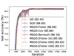
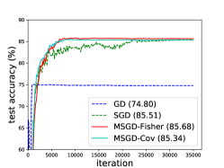
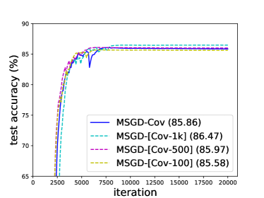
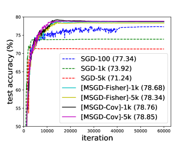
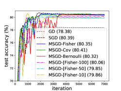
Figure 1: The generalization of MSGD. X-axis: number of iterations; y-axis: test accuracy. (a): We randomly draw 1,00010001,000 samples from FashionMNIST as the training set, then train a small convolutional network with them. (b): We use 25,0002500025,000 samples from SVHN as the training set, then train a VGG-11 without Batch Normalization. (c): We train a ResNet-18 on CIFAR-10 without using data augmentation and weight decay. MSGD-Fisher: MSGD with Gaussian gradient noise whose covariance is the scaled Fisher. MSGD-Cov: MSGD with Gaussian gradient noise whose covariance is the SGD covariance. MSGD-Bernoulli: MSGD with Bernoulli sampling noise. MSGD-[Fisher-𝐁𝐁\mathbf{B}]: MSGD-Fisher with the Fisher estimated using a mini-batch of samples in size B𝐵B.
Remark.

In the traditional setting of machine learning, the number of samples is much larger than the number of parameters, dnmuch-less-than𝑑𝑛d\ll n. And the SVD method for generating Gaussian noises is indeed plausible in this case. However, when it comes to deep neural networks where ndmuch-less-than𝑛𝑑n\ll d, it turns out computing the full gradient could be much cheaper than explicitly evaluating the covariance matrix and performing SVD. Thus for modern machine learning, our approach is far more efficient than the SVD method for injecting Gaussian noises with the SGD covariance.

Experiments  In Figure 1 we test MSGD-Cov on various datasets and models. The results consistently suggest that the MSGD-Cov can generalize well as the vanilla SGD, though its noise belongs to a different distribution class. More interestingly, we observe that the MSGD-Cov converges faster than the vanilla SGD.

4.2 Fisher vs. SGD covariance

In this part we discuss two kinds of commonly used Gaussian noises: the Gaussian noises with covariance as the SGD covariance, i.e., υC(θ)𝒩(0,C(θ))similar-tosubscript𝜐C𝜃𝒩0𝐶𝜃\upsilon_{\text{C}}(\theta)\sim\mathcal{N}(0,C(\theta)) (Zhu et al., 2018) and the scaled Fisher, i.e., υF(θ)𝒩(0,1bF(θ))similar-tosubscript𝜐F𝜃𝒩01𝑏𝐹𝜃\upsilon_{\text{F}}(\theta)\sim\mathcal{N}(0,\frac{1}{b}F(\theta)), where F(θ)=1nθ(θ)θ(θ)T𝐹𝜃1𝑛subscript𝜃𝜃subscript𝜃superscript𝜃𝑇F(\theta)=\frac{1}{n}\operatorname{\nabla}_{\theta}\mathcal{L}(\theta)\operatorname{\nabla}_{\theta}\mathcal{L}(\theta)^{T} is the Fisher. We call the MSGD with these two noises the MSGD-Cov and the MSGD-Fisher, respectively. The two noises sometimes cause confusion in literature, since both of them are adopted for simulating the SGD noise (Zhu et al., 2018; Wen et al., 2019); but we are not sure whether or not they have the same regularization effects (Martens, 2014; Kunstner et al., 2019; Thomas et al., 2019). The connection between the SGD covariance and the Fisher is clear: C(θ)=1b(F(θ)θL(θ)θL(θ)T)𝐶𝜃1𝑏𝐹𝜃subscript𝜃𝐿𝜃subscript𝜃𝐿superscript𝜃𝑇C(\theta)=\frac{1}{b}(F(\theta)-\operatorname{\nabla}_{\theta}L(\theta)\operatorname{\nabla}_{\theta}L(\theta)^{T}), i.e., ignoring a factor of scaling, C(θ)𝐶𝜃C(\theta) is the second central moment of the SGD noise, while F(θ)𝐹𝜃F(\theta) is the second raw moment. Next we discuss their common ground on imposing regularization.

Intuitively the two dynamics should not be far away from each other. We can see this by investigating the MSGD iteration (2). At the early phase of the training, the gradient term is much larger than the noise term in scale (Shwartz-Ziv & Tishby, 2017) and dominates the optimization. Thus the noise term almost makes no contribution, no matter whether its covariance is the SGD covariance or the scaled Fisher. During the latter phase, however, the gradient turns to be close to zero, thus C(θ)1bF(θ)𝐶𝜃1𝑏𝐹𝜃C(\theta)\approx\frac{1}{b}F(\theta) and υC(θ)υF(θ)subscript𝜐C𝜃subscript𝜐F𝜃\upsilon_{\text{C}}(\theta)\approx\upsilon_{\text{F}}(\theta). However, by such discussion neither the approximation is clear nor do we know about the transition phase.

Thanks to the sampling noise, we are able to develop a mathematical equivalence between the two noises along the whole training phase. Let 𝒱Csubscript𝒱C\mathcal{V}_{\text{C}} and 𝒱Fsubscript𝒱F\mathcal{V}_{\text{F}} be the sampling noises for υC(θ)subscript𝜐C𝜃\upsilon_{\text{C}}(\theta) and υF(θ)subscript𝜐F𝜃\upsilon_{\text{F}}(\theta) respectively, i.e., υC(θ)=θ(θ)𝒱Csubscript𝜐C𝜃subscript𝜃𝜃subscript𝒱C\upsilon_{\text{C}}(\theta)=\operatorname{\nabla}_{\theta}\mathcal{L}(\theta)\mathcal{V}_{\text{C}} and υF(θ)=θ(θ)𝒱Fsubscript𝜐F𝜃subscript𝜃𝜃subscript𝒱F\upsilon_{\text{F}}(\theta)=\operatorname{\nabla}_{\theta}\mathcal{L}(\theta)\mathcal{V}_{\text{F}}. By the MSGD algorithm we have

𝒱C=subscript𝒱Cabsent\displaystyle\mathcal{V}_{\text{C}}= 1bn(I1n𝟙𝟙T)ϵ=1bnϵ1bn𝟙Tϵn𝟙,1𝑏𝑛𝐼1𝑛superscript11𝑇italic-ϵ1𝑏𝑛italic-ϵ1𝑏𝑛superscript1𝑇italic-ϵ𝑛1\displaystyle\frac{1}{\sqrt{bn}}\left(I-\frac{1}{n}\mathbbm{1}\mathbbm{1}^{T}\right)\epsilon=\frac{1}{\sqrt{bn}}\epsilon-\frac{1}{\sqrt{bn}}\frac{\mathbbm{1}^{T}\epsilon}{n}\mathbbm{1},
𝒱F=subscript𝒱Fabsent\displaystyle\mathcal{V}_{\text{F}}= 1bnϵ,ϵ𝒩(0,In×n).similar-to1𝑏𝑛italic-ϵitalic-ϵ𝒩0subscript𝐼𝑛𝑛\displaystyle\frac{1}{\sqrt{bn}}\epsilon,\qquad\epsilon\sim\mathcal{N}(0,I_{n\times n}).

Note the matrix (I1N𝟙𝟙T)𝐼1𝑁superscript11𝑇\left(I-\frac{1}{N}\mathbbm{1}\mathbbm{1}^{T}\right) centralizes a random vector. But the components of the white noise ϵitalic-ϵ\epsilon are already i.i.d. of zero mean, thus 𝟙Tϵn0superscript1𝑇italic-ϵ𝑛0\frac{\mathbbm{1}^{T}\epsilon}{n}\approx 0 by the law of large numbers. Hence 𝒱C𝒱Fsubscript𝒱Csubscript𝒱F\mathcal{V}_{\text{C}}\approx\mathcal{V}_{\text{F}} and υC(θ)υF(θ)subscript𝜐C𝜃subscript𝜐F𝜃\upsilon_{\text{C}}(\theta)\approx\upsilon_{\text{F}}(\theta). Moreover, the equivalence holds no matter where the parameter θ𝜃\theta is, thanks to the fact that the sampling noises are state-independent. We conclude that the Fisher Gaussian noise and the SGD covariance noise must lead to identical regularization effect for learning deep models.

Experiments  In Figure 1 we present the experimental results regards MSGD-Cov and MSGD-Fisher. Consistent with our analysis, the behavior of the MSGD-Fisher perfectly approximates that of the MSGD-Cov. Hence the equivalence between the Fisher noise and the SGD covariance noise from the Gaussian class has been verified from both theory and experiments. In the following study, we focus on MSGD-Fisher as the representative of the algorithms with noises from the Gaussian class.

4.3 Bernoulli sampling noise

Notice that the Fisher sampling noise 𝒱Fsubscript𝒱F\mathcal{V}_{\text{F}} has i.i.d. components and loses the covariance structure of the SGD sampling noise. Nonetheless it can still regularize GD well (see MSGD-Fisher in Figure 1). It suggests that a sampling noise with independent components is capable enough for imposing regularization.

To further verify this conjecture, we consider a Bernoulli sampling noise: 𝒱B=(v1,,vn)Tsubscript𝒱Bsuperscriptsubscript𝑣1subscript𝑣𝑛𝑇\mathcal{V}_{\text{B}}=(v_{1},\dots,v_{n})^{T}, where the components are i.i.d. and (vi=1b1n)=bn,(vi=1n)=nbnformulae-sequencesubscript𝑣𝑖1𝑏1𝑛𝑏𝑛subscript𝑣𝑖1𝑛𝑛𝑏𝑛\mathbbm{P}(v_{i}=\frac{1}{b}-\frac{1}{n})=\frac{b}{n},\mathbbm{P}(v_{i}=-\frac{1}{n})=\frac{n-b}{n}. Then 𝔼[𝒱B]=0𝔼delimited-[]subscript𝒱B0\mathbbm{E}\left[\mathcal{V}_{\text{B}}\right]=0 and Var[𝒱B]=nbbn2I=Diag(Var[𝒱sgd])Varsubscript𝒱B𝑛𝑏𝑏superscript𝑛2𝐼DiagVardelimited-[]subscript𝒱sgd\operatorname{Var}[\mathcal{V}_{\text{B}}]=\frac{n-b}{bn^{2}}I=\operatorname{Diag}\left(\mathrm{Var}\left[\mathcal{V}_{\mathrm{sgd}}\right]\right), i.e., the covariance of the Bernoulli sampling noise is exactly the diagonal of the covariance of SGD sampling noise. The Bernuolli sampling noise can also be easily injected to GD by Algorithm 1, and we call such algorithm the MSGD-Bernoulli.

Experiments  In Figure 1 we find the MSGD-Bernoulli and the MSGD-Fisher both generalize as the vanilla SGD. Thus sampling noises with independent components do not lose the regularization ability. In contrast, gradient noises with independent components can never recover the regularization effects of the SGD noise. For example one can look at the performance of GLD diag in (Zhu et al., 2018). This comparison reveals a fundamental advantage of understanding the gradient noise from its sampling noise.
Refer to caption Refer to caption Refer to caption
(a) Small SVHN (b) CIFAR-10 (c) CIFAR-10 Standard
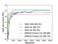
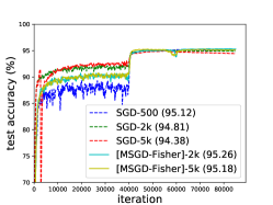
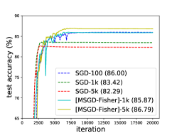
Figure 2: The generalization of mini-batch MSGD. X-axis: number of iterations; y-axis: test accuracy. (a): We use 25,0002500025,000 samples from SVHN as the training set, then train a VGG-11 without Batch Normalization. (b): We train a ResNet-18 on CIFAR-10 without using data augmentation and weight decay. (c): We train a ResNet-18 on CIFAR-10 with full tricks. SGD-𝐁𝐁\mathbf{B}: SGD with batch size B𝐵B. [MSGD-Fisher]-𝐁𝐁\mathbf{B}: mini-batch MSGD with batch size B𝐵B, and an compensatory sampling noise from the (sparse) Gaussian class.

4.4 Sparse Gaussian sampling noises

We then study another class of gradient noise who has sparse Gaussian sampling noise. The gradient noise is constructed as below: we first draw a mini-batch of samples uniformly at random in size B𝐵B, then estimate the Fisher using this mini-batch, then generate a Gaussian noise using the estimated Fisher as covariance, finally the noise is properly scaled to maintain the magnitude. By Algorithm 1, the sampling noise is generated as

𝒱F=B/b𝒱sgd(B)ϵ,superscriptsubscript𝒱𝐹direct-product𝐵𝑏subscript𝒱sgd𝐵italic-ϵ\mathcal{V}_{F}^{\prime}=\sqrt{B/b}\cdot\mathcal{V}_{\mathrm{sgd}}(B)\odot\epsilon,

where 𝒱sgd(B)subscript𝒱sgd𝐵\mathcal{V}_{\mathrm{sgd}}(B) is the SGD sampling noise with batch size B𝐵B, and ϵnitalic-ϵsuperscript𝑛\epsilon\in\mathbbm{R}^{n} is a white noise. MSGD using 𝒱Fsuperscriptsubscript𝒱𝐹\mathcal{V}_{F}^{\prime} as sampling noise is denoted as MSGD-[Fisher-B𝐵B], where B𝐵B is the batch size. Note that 𝔼[𝒱F]=0𝔼delimited-[]superscriptsubscript𝒱𝐹0\mathbbm{E}[\mathcal{V}_{F}^{\prime}]=0 and Var[𝒱F]=Var[𝒱sgd(b)]Varsuperscriptsubscript𝒱𝐹Varsubscript𝒱sgd𝑏\operatorname{Var}[\mathcal{V}_{F}^{\prime}]=\operatorname{Var}[\mathcal{V}_{\mathrm{sgd}}(b)], i.e., the sampling noise has the same magnitude and covariance structure as the SGD sampling noise. Because 𝒱Fsuperscriptsubscript𝒱𝐹\mathcal{V}_{F}^{\prime} is a sparse Gaussian noise, its gradient noise belongs to neither the Gaussian class nor the SGD noise class.

Experiments  The performance of MSGD-[Fisher-B𝐵B] is shown in Figures 1. Even with a very small batch size, e.g., 101010 for FashionMNIST and 100100100 for SVHN, MSGD-[Fisher-B𝐵B] can generalize as MSGD-Fisher and SGD. These results further support our understanding that the noise class is not the crux for regularization.

4.5 Mini-batch MSGD

Finally, we discuss the mini-batch version of MSGD which is of practical interests. During each iteration of the vanilla MSGD, the information of full training set is required, which is unacceptable in practice. As an extension, we introduce Algorithm 2, the mini-batch MSGD. For example, when the plugged noise is Fisher Gaussian noise, we call the algorithm [MSGD-Fisher]-B𝐵B, where B𝐵B denotes the batch size of the mini-batch MSGD algorithm. We emphasize that the sampling noise in [MSGD-Fisher]-B𝐵B is a sparse Gaussian noise plus an SGD sampling noise, thus it belongs to a new class different from what we have discussed before. However, thanks to the fact that noise class is unimportant the regularization ability, the noises we adopt here do not limit the capability of the mini-batch MSGD.

Algorithm 2 Mini-Batch Multiplicative SGD
1:  Input: Initial parameter θ0dsubscript𝜃0superscript𝑑\theta_{0}\in\mathbb{R}^{d}, training data {(xi,yi)}i=1nsuperscriptsubscriptsubscript𝑥𝑖subscript𝑦𝑖𝑖1𝑛\{(x_{i},y_{i})\}_{i=1}^{n}, loss function i(θ)=((xi,yi),θ)subscript𝑖𝜃subscript𝑥𝑖subscript𝑦𝑖𝜃\ell_{i}(\theta)=\ell((x_{i},y_{i}),\theta)\in\mathbbm{R}, learning rate η>0𝜂0\eta>0, batch size b𝑏b
2:  for k=0,1,2,,K1𝑘012𝐾1k=0,1,2,...,K-1 do
3:     Uniformly sample a mini-batch {k1,,kb}subscript𝑘1subscript𝑘𝑏\{k_{1},\dots,k_{b}\} and collect the loss vector (θk)=(k1(θk),,kb(θk))1×bsubscript𝜃𝑘subscriptsubscript𝑘1subscript𝜃𝑘subscriptsubscript𝑘𝑏subscript𝜃𝑘superscript1𝑏\mathcal{L}(\theta_{k})=\left(\ell_{k_{1}}(\theta_{k}),\dots,\ell_{k_{b}}(\theta_{k})\right)\in\mathbbm{R}^{1\times b}
4:     Generate a sampling noise 𝒱b𝒱superscript𝑏\mathcal{V}\in\mathbbm{R}^{b} of zero mean and desired covariance
5:     Compute the sampling vector 𝒲=1b𝟙+𝒱𝒲1𝑏1𝒱\mathcal{W}=\frac{1}{b}\mathbbm{1}+\mathcal{V}
6:     Calculate the randomized loss L~(θk)=(θk)𝒲~𝐿subscript𝜃𝑘subscript𝜃𝑘𝒲\tilde{L}(\theta_{k})=\mathcal{L}(\theta_{k})\mathcal{W}
7:     Compute the stochastic gradient θL~(θk)subscript𝜃~𝐿subscript𝜃𝑘\operatorname{\nabla}_{\theta}\tilde{L}(\theta_{k})
8:     Update the parameter θk+1=θkηθL~(θk)subscript𝜃𝑘1subscript𝜃𝑘𝜂subscript𝜃~𝐿subscript𝜃𝑘\theta_{k+1}=\theta_{k}-\eta\operatorname{\nabla}_{\theta}\tilde{L}(\theta_{k})
9:  end for
10:  Output: Output θKsubscript𝜃𝐾\theta_{K}

Large batch training  When training with SGD, as the batch size becomes large, the generalization gets hurt since the gradient noise tends to be small  (Keskar et al., 2017). A promising method to close the generalization gap of large batch training is adding a compensatory gradient noise, e.g., a Gaussian gradient noise using scaled Fisher as covariance (Wen et al., 2019). However as we have discussed in Section 4.1, it is computationally costly to directly insert a structured Gaussian noise via SVD. Instead, the algorithm [MSGD-Fisher]-B𝐵B provides an efficient method for injecting a compensatory sampling noise from the (sparse) Gaussian class.

Experiments  We thus perform large batch training experiments with our [MSGD-Fisher]-B𝐵B algorithm. The results are shown in Figure 2. Since in this case the covariance of the sampling noise becomes hard to calculate, we simply tune the noise magnitude to achieve its best performance. As illustrated in Figure 2 (a) (b), on toy datasets the [MSGD-Fisher]-B𝐵B with large batch size has a even better generalization compared with small batch SGD. Its convergence is also faster. Even in real settings of training ResNet-18 on CIFAR10, Figure 2 (c) demonstrates that the [MSGD-Fisher]-B𝐵B with large batch size generalizes well as the small batch SGD, while SGD with large batch size performs worse.

4.6 Empirical studies summary

In Figure 1 we compare the generalization performance of noisy gradient descents with noises from various different classes. We find that, provide suitable magnitude and covariance structure, all the concerned noises can regularize gradient descent as the SGD noise. These empirical results together with the theoretical evidence verify our understanding that the noise class is not a crux for regularization. An interesting additional finding is that Gaussian MSGD tends to converge faster than others.

In Figure 2 we present the empirical results of the mini-batch MSGD (Algorithm 2). Our algorithm perfectly closes the generalization gap of large batch training by injecting compensatory (sparse) Gaussian sampling noises. Besides, our algorithm achieves this effect in a more efficient manner than the traditional way of inserting Gaussian gradient noise based on SVD. These results demonstrate the promising application of the mini-batch MSGD algorithm in practice.

5 Discussion

Benefits of Gaussian gradient noise  The continuous stochastic differential equations (SDEs) have been widely used for approximating and analyzing the discrete SGD iterations (Li et al., 2017; Hu et al., 2017; Orvieto & Lucchi, 2019). For SGD, this continuous approximation only hold in weak sense (Li et al., 2017). For Gaussian MSGD, however, a strong convergence can be established between the discrete iterations and the continuous SDEs. This is discussed more in Supplementary Materials, Section B. The strong convergence guarantees a path-wise closeness between the discrete iterations and the continuous paths, beyond the close behavior at the level of probability distributions guaranteed by weak convergence. This advantage of Gaussian MSGD might account for its observed faster convergence.

The importance of the gradient matrix θ(θ)subscript𝜃𝜃\operatorname{\nabla}_{\theta}\mathcal{L}(\theta)  Consider the MSGD-Bernoulli/Fisher and the GLD diag from (Zhu et al., 2018), empirical studies show that the MSGD-Bernoulli/Fisher generalize well as SGD, while the GLD diag performs much worse. In the MSGD-Bernoulli/Fisher the sampling noises have independent components, and in the GLD diag the gradient noise has independent components. Though the compared algorithms all discard certain “dependece” in their noises, the MSGD-Bernoulli/Fisher keep the full information of the gradient matrix, while the GLD diag severally destroys its structure. We thus conjecture that the gradient matrix contains key information for the regularization induced by noises.

6 Conclusion

In this work we introduce a novel kind of gradient noise as the composition of the gradient matrix and a sampling noise, which includes the SGD noise. By investigating these noises we find the noise class is not a crux for regularization, provided suitable noise magnitude and covariance structure. Furthermore, we show that the scaled Fisher and the gradient covariance of SGD is equivalent when serve as the covariance of noises from the Gaussian class. Finally, an algorithm is proposed to perform noisy gradient descent that generalizes as SGD. The algorithm can be extended for practical usage like large batch training.

Acknowledgement

This project is supported by National Natural Science Foundation of China (No.61806009 and 61932001), PKU-Baidu Funding 2019BD005, Beijing Academy of Artificial Intelligence (BAAI), Intelligent Manufacturing Action Plan of Industrial Solid Foundation Program (JCKY2018204C004), NSF CAREER grant 1652257, ONR Award N00014-18-1-2364, and the Lifelong Learning Machines program from DARPA/MTO.

References

  • Ahn et al. (2012) Ahn, S., Korattikara, A., and Welling, M. Bayesian posterior sampling via stochastic gradient fisher scoring. In Proceedings of the 29th International Coference on International Conference on Machine Learning, pp.  1771–1778. Omnipress, 2012.
  • Bach & Moulines (2013) Bach, F. and Moulines, E. Non-strongly-convex smooth stochastic approximation with convergence rate o (1/n). In Advances in neural information processing systems, pp. 773–781, 2013.
  • Bertoin (1998) Bertoin, J. Levy Processes (Cambridge Tracts in Mathematics). Cambridge University Press, 1998.
  • Borkar & Mitter (1999) Borkar, V. S. and Mitter, S. K. A strong approximation theorem for stochastic recursive algorithms. Journal of optimization theory and applications, 100(3):499–513, 1999.
  • Bottou (1991) Bottou, L. Stochastic gradient learning in neural networks. Proceedings of Neuro-Nımes, 91(8), 1991.
  • Bottou et al. (2018) Bottou, L., Curtis, F. E., and Nocedal, J. Optimization methods for large-scale machine learning. Siam Review, 60(2):223–311, 2018.
  • Cao & Gu (2019) Cao, Y. and Gu, Q. Generalization bounds of stochastic gradient descent for wide and deep neural networks. In Advances in Neural Information Processing Systems, pp. 10835–10845, 2019.
  • Chaudhari & Soatto (2017) Chaudhari, P. and Soatto, S. Stochastic gradient descent performs variational inference, converges to limit cycles for deep networks. arXiv preprint arXiv:1710.11029, 2017.
  • Chen et al. (2014) Chen, T., Fox, E., and Guestrin, C. Stochastic gradient hamiltonian monte carlo. In International Conference on Machine Learning, pp. 1683–1691, 2014.
  • Daneshmand et al. (2018) Daneshmand, H., Kohler, J., Lucchi, A., and Hofmann, T. Escaping saddles with stochastic gradients. arXiv preprint arXiv:1803.05999, 2018.
  • Défossez & Bach (2015) Défossez, A. and Bach, F. Averaged least-mean-squares: Bias-variance trade-offs and optimal sampling distributions. In Artificial Intelligence and Statistics, pp.  205–213, 2015.
  • Dieuleveut et al. (2017) Dieuleveut, A., Flammarion, N., and Bach, F. Harder, better, faster, stronger convergence rates for least-squares regression. The Journal of Machine Learning Research, 18(1):3520–3570, 2017.
  • Gnedenko & Kolmogorov (1968) Gnedenko, B. and Kolmogorov, A. Limit Distributions for Sums of Independent Random Variables (English translation by K. L. Chung). Addison-Wesley, 1968.
  • Goodfellow et al. (2016) Goodfellow, I., Bengio, Y., and Courville, A. Deep learning. MIT press, 2016.
  • Hochreiter & Schmidhuber (1997) Hochreiter, S. and Schmidhuber, J. Flat minima. Neural Computation, 9(1):1–42, 1997.
  • Hoffer et al. (2017) Hoffer, E., Hubara, I., and Soudry, D. Train longer, generalize better: closing the generalization gap in large batch training of neural networks. In Guyon, I., Luxburg, U. V., Bengio, S., Wallach, H., Fergus, R., Vishwanathan, S., and Garnett, R. (eds.), Advances in Neural Information Processing Systems 30, pp.  1731–1741. Curran Associates, Inc., 2017.
  • Hu et al. (2017) Hu, W., Junchi Li, C., Li, L., and Liu, J.-G. On the diffusion approximation of nonconvex stochastic gradient descent. arXiv preprint arXiv:1705.07562, 2017.
  • Hu et al. (2019) Hu, W., Zhu, Z., Xiong, H., and Huan, J. Quasi-potential as an implicit regularizer for the loss function in the stochastic gradient descent. arXiv preprint arXiv:1901.06054, 2019.
  • Huang et al. (2017) Huang, G., Liu, Z., Van Der Maaten, L., and Weinberger, K. Q. Densely connected convolutional networks. In Proceedings of the IEEE conference on computer vision and pattern recognition, pp.  4700–4708, 2017.
  • Jacot et al. (2018) Jacot, A., Gabriel, F., and Hongler, C. Neural tangent kernel: Convergence and generalization in neural networks. In Advances in neural information processing systems, pp. 8571–8580, 2018.
  • Jastrzębski et al. (2017) Jastrzębski, S., Kenton, Z., Arpit, D., Ballas, N., Fischer, A., Bengio, Y., and Storkey, A. Three factors influencing minima in sgd. arXiv preprint arXiv:1711.04623, 2017.
  • Keskar et al. (2017) Keskar, N. S., Mudigere, D., Nocedal, J., Smelyanskiy, M., and Tang, P. T. P. On large-batch training for deep learning: Generalization gap and sharp minima. In In International Conference on Learning Representations (ICLR), 2017.
  • Kunstner et al. (2019) Kunstner, F., Hennig, P., and Balles, L. Limitations of the empirical fisher approximation for natural gradient descent. In Advances in Neural Information Processing Systems, pp. 4158–4169, 2019.
  • Li et al. (2017) Li, Q., Tai, C., and Weinan, E. Stochastic modified equations and adaptive stochastic gradient algorithms. In International Conference on Machine Learning, pp. 2101–2110, 2017.
  • Li et al. (2019) Li, X., Gu, Q., Zhou, Y., Chen, T., and Banerjee, A. Hessian based analysis of sgd for deep nets: Dynamics and generalization. arXiv preprint arXiv:1907.10732, 2019.
  • Mandt et al. (2017) Mandt, S., Hoffman, M. D., and Blei, D. M. Stochastic gradient descent as approximate bayesian inference. The Journal of Machine Learning Research, 18(1):4873–4907, 2017.
  • Martens (2014) Martens, J. New insights and perspectives on the natural gradient method, 2014.
  • Martens & Grosse (2015) Martens, J. and Grosse, R. Optimizing neural networks with kronecker-factored approximate curvature. In International conference on machine learning, pp. 2408–2417, 2015.
  • Neyshabur et al. (2017) Neyshabur, B., Bhojanapalli, S., Mcallester, D., and Srebro, N. Exploring generalization in deep learning. In Guyon, I., Luxburg, U. V., Bengio, S., Wallach, H., Fergus, R., Vishwanathan, S., and Garnett, R. (eds.), Advances in Neural Information Processing Systems 30, pp.  5947–5956. Curran Associates, Inc., 2017.
  • Nguyen et al. (2019) Nguyen, T. H., Şimşekli, U., Gürbüzbalaban, M., and Richard, G. First exit time analysis of stochastic gradient descent under heavy-tailed gradient noise. arXiv preprint arXiv:1906.09069, 2019.
  • Øksendal (2003) Øksendal, B. Stochastic differential equations. In Stochastic differential equations, pp.  65–84. Springer, 2003.
  • Orvieto & Lucchi (2019) Orvieto, A. and Lucchi, A. Continuous-time models for stochastic optimization algorithms. In Advances in Neural Information Processing Systems, pp. 12589–12601, 2019.
  • Panigrahi et al. (2019) Panigrahi, A., Somani, R., Goyal, N., and Netrapalli, P. Non-gaussianity of stochastic gradient noise. arXiv preprint arXiv:1910.09626, 2019.
  • Shang et al. (2015) Shang, X., Zhu, Z., Leimkuhler, B., and Storkey, A. J. Covariance-controlled adaptive langevin thermostat for large-scale bayesian sampling. In Advances in Neural Information Processing Systems, pp. 37–45, 2015.
  • Shwartz-Ziv & Tishby (2017) Shwartz-Ziv, R. and Tishby, N. Opening the black box of deep neural networks via information. arXiv preprint arXiv:1703.00810, 2017.
  • Şimşekli et al. (2019) Şimşekli, U., Gürbüzbalaban, M., Nguyen, T. H., Richard, G., and Sagun, L. On the heavy-tailed theory of stochastic gradient descent for deep neural networks. arXiv preprint arXiv:1912.00018, 2019.
  • Simsekli et al. (2019) Simsekli, U., Sagun, L., and Gurbuzbalaban, M. A tail-index analysis of stochastic gradient noise in deep neural networks. arXiv preprint arXiv:1901.06053, 2019.
  • Smith & Le (2018) Smith, S. L. and Le, Q. V. A bayesian perspective on generalization and stochastic gradient descent. International Conference on Learning Representations, 2018. URL https://openreview.net/forum?id=BJij4yg0Z.
  • Thomas et al. (2019) Thomas, V., Pedregosa, F., van Merriënboer, B., Mangazol, P.-A., Bengio, Y., and Roux, N. L. On the interplay between noise and curvature and its effect on optimization and generalization, 2019.
  • Wen et al. (2019) Wen, Y., Luk, K., Gazeau, M., Zhang, G., Chan, H., and Ba, J. Interplay between optimization and generalization of stochastic gradient descent with covariance noise, 2019.
  • Zhang et al. (2017) Zhang, C., Bengio, S., Hardt, M., Recht, B., and Vinyals, O. Understanding deep learning requires rethinking generalization. In International Conference on Learning Representations, 2017.
  • Zhu et al. (2018) Zhu, Z., Wu, J., Yu, B., Wu, L., and Ma, J. The anisotropic noise in stochastic gradient descent: Its behavior of escaping from minima and regularization effects. arXiv preprint arXiv:1803.00195, 2018.

Appendix A Missing proofs in main paper

A.1 Proof of Proposition 1

Proof.

We first calculate the expectation and variance of the sampling random vector 𝒲sgdsubscript𝒲sgd\mathcal{W}_{\mathrm{sgd}}, then obtain that of the sampling noise 𝒱sgdsubscript𝒱sgd\mathcal{V}_{\mathrm{sgd}}.

Sampling with replacement

In the circumstance of sampling with replacement, the sampling random vector 𝒲sgdsubscript𝒲sgd\mathcal{W}_{\mathrm{sgd}} could be decompose as

𝒲sgd=𝒲1++𝒲b,subscript𝒲sgdsuperscript𝒲1superscript𝒲𝑏\mathcal{W}_{\mathrm{sgd}}=\mathcal{W}^{1}+\dots+\mathcal{W}^{b},

where 𝒲1,,𝒲bsuperscript𝒲1superscript𝒲𝑏\mathcal{W}^{1},\dots,\mathcal{W}^{b} are i.i.d. and each of them represents once sampling procedure. Thus 𝒲i=(w1i,,wni)Tsuperscript𝒲𝑖superscriptsubscriptsuperscript𝑤𝑖1subscriptsuperscript𝑤𝑖𝑛𝑇\mathcal{W}^{i}=(w^{i}_{1},\dots,w^{i}_{n})^{T} contains one multiple of 1b1𝑏\frac{1}{b} and n1𝑛1n-1 multiples of zero, with random index. Hence we have

𝔼[wji]=1bn,𝔼[wjiwji]=1b2n,𝔼[wjiwki]=0,jk.formulae-sequence𝔼delimited-[]subscriptsuperscript𝑤𝑖𝑗1𝑏𝑛formulae-sequence𝔼delimited-[]subscriptsuperscript𝑤𝑖𝑗subscriptsuperscript𝑤𝑖𝑗1superscript𝑏2𝑛formulae-sequence𝔼delimited-[]subscriptsuperscript𝑤𝑖𝑗subscriptsuperscript𝑤𝑖𝑘0for-all𝑗𝑘\mathbbm{E}[w^{i}_{j}]=\frac{1}{bn},\quad\mathbbm{E}[w^{i}_{j}w^{i}_{j}]=\frac{1}{b^{2}n},\quad\mathbbm{E}[w^{i}_{j}w^{i}_{k}]=0,\ \forall j\neq k.

Thus

𝔼[𝒲i]=𝔼delimited-[]superscript𝒲𝑖absent\displaystyle\mathbbm{E}[\mathcal{W}^{i}]= 1bn𝟙,1𝑏𝑛1\displaystyle\frac{1}{bn}\mathbbm{1},
Var[𝒲i]=Varsuperscript𝒲𝑖absent\displaystyle\operatorname{Var}[\mathcal{W}^{i}]= 𝔼[𝒲i(𝒲i)T]𝔼[𝒲i]𝔼[𝒲i]T=(1b2n1b2n)1b2n2𝟙𝟙T=1b2n(I1n𝟙𝟙T).𝔼delimited-[]superscript𝒲𝑖superscriptsuperscript𝒲𝑖𝑇𝔼delimited-[]superscript𝒲𝑖𝔼superscriptdelimited-[]superscript𝒲𝑖𝑇matrix1superscript𝑏2𝑛missing-subexpressionmissing-subexpressionmissing-subexpressionmissing-subexpressionmissing-subexpressionmissing-subexpression1superscript𝑏2𝑛1superscript𝑏2superscript𝑛2superscript11𝑇1superscript𝑏2𝑛𝐼1𝑛superscript11𝑇\displaystyle\mathbbm{E}[\mathcal{W}^{i}(\mathcal{W}^{i})^{T}]-\mathbbm{E}[\mathcal{W}^{i}]\mathbbm{E}[\mathcal{W}^{i}]^{T}=\begin{pmatrix}\frac{1}{b^{2}n}&&\\ &\ddots&\\ &&\frac{1}{b^{2}n}\end{pmatrix}-\frac{1}{b^{2}n^{2}}\mathbbm{1}\mathbbm{1}^{T}=\frac{1}{b^{2}n}\left(I-\frac{1}{n}\mathbbm{1}\mathbbm{1}^{T}\right).

Recall 𝒲1,,𝒲bsuperscript𝒲1superscript𝒲𝑏\mathcal{W}^{1},\dots,\mathcal{W}^{b} are i.i.d., thus

𝔼[𝒲sgd]=b𝔼[𝒲i]=1n𝟙,Var[𝒲sgd]=bVar[𝒲i]=1bn(I1n𝟙𝟙T).formulae-sequence𝔼delimited-[]subscript𝒲sgd𝑏𝔼delimited-[]superscript𝒲𝑖1𝑛1Varsubscript𝒲sgd𝑏Varsuperscript𝒲𝑖1𝑏𝑛𝐼1𝑛superscript11𝑇\mathbbm{E}[\mathcal{W}_{\mathrm{sgd}}]=b\mathbbm{E}[\mathcal{W}^{i}]=\frac{1}{n}\mathbbm{1},\quad\operatorname{Var}[\mathcal{W}_{\mathrm{sgd}}]=b\operatorname{Var}[\mathcal{W}^{i}]=\frac{1}{bn}\left(I-\frac{1}{n}\mathbbm{1}\mathbbm{1}^{T}\right).

Therefore for the sampling noise 𝒱sgd=𝒲sgd1n𝟙subscript𝒱sgdsubscript𝒲sgd1𝑛1\mathcal{V}_{\mathrm{sgd}}=\mathcal{W}_{\mathrm{sgd}}-\frac{1}{n}\mathbbm{1} we have

𝔼[𝒱sgd]=0,Var[𝒱sgd]=1bn(I1n𝟙𝟙T).formulae-sequence𝔼delimited-[]subscript𝒱sgd0Varsubscript𝒱sgd1𝑏𝑛𝐼1𝑛superscript11𝑇\mathbbm{E}[\mathcal{V}_{\mathrm{sgd}}]=0,\quad\operatorname{Var}[\mathcal{V}_{\mathrm{sgd}}]=\frac{1}{bn}\left(I-\frac{1}{n}\mathbbm{1}\mathbbm{1}^{T}\right).

Sampling without replacement

Let 𝒲sgd=(w1,,wn)Tsuperscriptsubscript𝒲sgdsuperscriptsubscriptsuperscript𝑤1subscriptsuperscript𝑤𝑛𝑇\mathcal{W}_{\mathrm{sgd}}^{\prime}=(w^{\prime}_{1},\dots,w^{\prime}_{n})^{T}. In the case of sampling without replacement, we know the sampling random vector 𝒲sgdsuperscriptsubscript𝒲sgd\mathcal{W}_{\mathrm{sgd}}^{\prime} contains exactly b𝑏b multiples of 1b1𝑏\frac{1}{b}s and nb𝑛𝑏n-b multiples of zero, with random index. Hence we have

𝔼[wj]=(n1b1)1b(nb)=1n,𝔼[(wj)2]=(n1b1)1b2(nb)=1bn,𝔼[wjwk]=(n2b2)1b2(nb)=b1bn(n1),jk.formulae-sequence𝔼delimited-[]subscriptsuperscript𝑤𝑗binomial𝑛1𝑏11𝑏binomial𝑛𝑏1𝑛𝔼delimited-[]superscriptsubscriptsuperscript𝑤𝑗2binomial𝑛1𝑏11superscript𝑏2binomial𝑛𝑏1𝑏𝑛𝔼delimited-[]subscriptsuperscript𝑤𝑗subscriptsuperscript𝑤𝑘binomial𝑛2𝑏21superscript𝑏2binomial𝑛𝑏𝑏1𝑏𝑛𝑛1for-all𝑗𝑘\mathbbm{E}[w^{\prime}_{j}]=\frac{\binom{n-1}{b-1}\frac{1}{b}}{\binom{n}{b}}=\frac{1}{n},\quad\mathbbm{E}[(w^{\prime}_{j})^{2}]=\frac{\binom{n-1}{b-1}\frac{1}{b^{2}}}{\binom{n}{b}}=\frac{1}{bn},\quad\mathbbm{E}[w^{\prime}_{j}w^{\prime}_{k}]=\frac{\binom{n-2}{b-2}\frac{1}{b^{2}}}{\binom{n}{b}}=\frac{b-1}{bn(n-1)},\ \forall j\neq k.

Thus

𝔼[𝒲sgd]=𝔼delimited-[]superscriptsubscript𝒲sgdabsent\displaystyle\mathbbm{E}[\mathcal{W}_{\mathrm{sgd}}^{\prime}]= 1N𝟙,1𝑁1\displaystyle\frac{1}{N}\mathbbm{1},
Var[𝒲sgd]=Varsuperscriptsubscript𝒲sgdabsent\displaystyle\operatorname{Var}[\mathcal{W}_{\mathrm{sgd}}^{\prime}]= 𝔼[𝒲sgd(𝒲sgd)T]𝔼[𝒲i]𝔼[𝒲i]T𝔼delimited-[]superscriptsubscript𝒲sgdsuperscriptsuperscriptsubscript𝒲sgd𝑇𝔼delimited-[]superscript𝒲𝑖𝔼superscriptdelimited-[]superscript𝒲𝑖𝑇\displaystyle\mathbbm{E}[\mathcal{W}_{\mathrm{sgd}}^{\prime}(\mathcal{W}_{\mathrm{sgd}}^{\prime})^{T}]-\mathbbm{E}[\mathcal{W}^{i}]\mathbbm{E}[\mathcal{W}^{i}]^{T}
=\displaystyle= (1bnb1bn(n1)b1bn(n1)b1bn(n1)1bnb1bn(n1)b1bn(n1)b1bn(n1)1b2n)1n2𝟙𝟙T=nbbn(n1)(I1n𝟙𝟙T).matrix1𝑏𝑛𝑏1𝑏𝑛𝑛1𝑏1𝑏𝑛𝑛1𝑏1𝑏𝑛𝑛11𝑏𝑛𝑏1𝑏𝑛𝑛1𝑏1𝑏𝑛𝑛1𝑏1𝑏𝑛𝑛11superscript𝑏2𝑛1superscript𝑛2superscript11𝑇𝑛𝑏𝑏𝑛𝑛1𝐼1𝑛superscript11𝑇\displaystyle\begin{pmatrix}\frac{1}{bn}&\frac{b-1}{bn(n-1)}&\cdots&\frac{b-1}{bn(n-1)}\\ \frac{b-1}{bn(n-1)}&\frac{1}{bn}&\cdots&\frac{b-1}{bn(n-1)}\\ \vdots&\vdots&\ddots&\vdots\\ \frac{b-1}{bn(n-1)}&\frac{b-1}{bn(n-1)}&\cdots&\frac{1}{b^{2}n}\end{pmatrix}-\frac{1}{n^{2}}\mathbbm{1}\mathbbm{1}^{T}=\frac{n-b}{bn(n-1)}\left(I-\frac{1}{n}\mathbbm{1}\mathbbm{1}^{T}\right).

Therefore for the sampling noise 𝒱sgd=𝒲sgd1n𝟙superscriptsubscript𝒱sgdsuperscriptsubscript𝒲sgd1𝑛1\mathcal{V}_{\mathrm{sgd}}^{\prime}=\mathcal{W}_{\mathrm{sgd}}^{\prime}-\frac{1}{n}\mathbbm{1} we have

𝔼[𝒱sgd]=0,Var[𝒱sgd]=nbbn(n1)(I1n𝟙𝟙T).formulae-sequence𝔼delimited-[]superscriptsubscript𝒱sgd0Varsuperscriptsubscript𝒱sgd𝑛𝑏𝑏𝑛𝑛1𝐼1𝑛superscript11𝑇\mathbbm{E}[\mathcal{V}_{\mathrm{sgd}}^{\prime}]=0,\quad\operatorname{Var}[\mathcal{V}_{\mathrm{sgd}}^{\prime}]=\frac{n-b}{bn(n-1)}\left(I-\frac{1}{n}\mathbbm{1}\mathbbm{1}^{T}\right).

A.2 Proof of Theorem 1

Proof.

Let

ϵn=ynxnTθ,subscriptitalic-ϵ𝑛subscript𝑦𝑛superscriptsubscript𝑥𝑛𝑇subscript𝜃\epsilon_{n}=y_{n}-x_{n}^{T}\theta_{*},

by assumption we have

𝔼[ϵnxn]=0,𝔼[ϵn]=0,𝔼[ϵ2xxT]σ2Σ.formulae-sequence𝔼delimited-[]subscriptitalic-ϵ𝑛subscript𝑥𝑛0formulae-sequence𝔼delimited-[]subscriptitalic-ϵ𝑛0precedes-or-equals𝔼delimited-[]superscriptitalic-ϵ2𝑥superscript𝑥𝑇superscript𝜎2Σ\mathbbm{E}[\epsilon_{n}x_{n}]=0,\quad\mathbbm{E}[\epsilon_{n}]=0,\quad\mathbbm{E}[\epsilon^{2}xx^{T}]\preceq\sigma^{2}\Sigma.

Recall the MSGD updates

θn+1=θnηrBnwr(xrxrTθnyrxr),subscript𝜃𝑛1subscript𝜃𝑛𝜂subscript𝑟subscript𝐵𝑛subscript𝑤𝑟subscript𝑥𝑟superscriptsubscript𝑥𝑟𝑇subscript𝜃𝑛subscript𝑦𝑟subscript𝑥𝑟\theta_{n+1}=\theta_{n}-\eta\sum_{r\in B_{n}}w_{r}\left(x_{r}x_{r}^{T}\theta_{n}-y_{r}x_{r}\right),

hence we have

θn+1θ=(IηrBnwrxrxrT)(θnθ)+ηrBnwrϵrxr.subscript𝜃𝑛1subscript𝜃𝐼𝜂subscript𝑟subscript𝐵𝑛subscript𝑤𝑟subscript𝑥𝑟superscriptsubscript𝑥𝑟𝑇subscript𝜃𝑛subscript𝜃𝜂subscript𝑟subscript𝐵𝑛subscript𝑤𝑟subscriptitalic-ϵ𝑟subscript𝑥𝑟\theta_{n+1}-\theta_{*}=\left(I-\eta\sum_{r\in B_{n}}w_{r}x_{r}x_{r}^{T}\right)(\theta_{n}-\theta_{*})+\eta\sum_{r\in B_{n}}w_{r}\epsilon_{r}x_{r}.

Define

L(k)=rBkwrxrxrT,𝐿𝑘subscript𝑟subscript𝐵𝑘subscript𝑤𝑟subscript𝑥𝑟superscriptsubscript𝑥𝑟𝑇\displaystyle L(k)=\sum_{r\in B_{k}}w_{r}x_{r}x_{r}^{T}, (5)
M(i,k)={(IηL(i))(IηL(k)),ikI,i<k.𝑀𝑖𝑘casesotherwise𝐼𝜂𝐿𝑖𝐼𝜂𝐿𝑘𝑖𝑘otherwise𝐼𝑖𝑘\displaystyle M(i,k)=\begin{cases}&\left(I-\eta L(i)\right)\cdots\left(I-\eta L(k)\right),\quad i\geq k\\ &I,\quad i<k.\end{cases} (6)
N(k)=rBkwrϵrxr,𝑁𝑘subscript𝑟subscript𝐵𝑘subscript𝑤𝑟subscriptitalic-ϵ𝑟subscript𝑥𝑟\displaystyle N(k)=\sum_{r\in B_{k}}w_{r}\epsilon_{r}x_{r}, (7)

Then recursively we obtain

θiθ=M(i,1)(θ0θ)+ηk=1iM(i,k+1)N(k).subscript𝜃𝑖subscript𝜃𝑀𝑖1subscript𝜃0subscript𝜃𝜂superscriptsubscript𝑘1𝑖𝑀𝑖𝑘1𝑁𝑘\theta_{i}-\theta_{*}=M(i,1)(\theta_{0}-\theta_{*})+\eta\sum_{k=1}^{i}M(i,k+1)N(k). (8)

Moments of L(k)𝐿𝑘L(k)

We first calculate the first and second moments of N(k)𝑁𝑘N(k) defined in Eq. (7). Since 𝔼[wr]=1B,𝔼[wi2]=1bB,𝔼[wiwj]=b1bB(B1),ijformulae-sequence𝔼delimited-[]subscript𝑤𝑟1𝐵formulae-sequence𝔼delimited-[]superscriptsubscript𝑤𝑖21𝑏𝐵formulae-sequence𝔼delimited-[]subscript𝑤𝑖subscript𝑤𝑗𝑏1𝑏𝐵𝐵1𝑖𝑗\mathbbm{E}[w_{r}]=\frac{1}{B},\ \mathbbm{E}[w_{i}^{2}]=\frac{1}{bB},\ \mathbbm{E}[w_{i}w_{j}]=\frac{b-1}{bB(B-1)},\ i\neq j, and 𝔼[x22xxT]R2Σ,ΣλIformulae-sequenceprecedes-or-equals𝔼delimited-[]superscriptsubscriptnorm𝑥22𝑥superscript𝑥𝑇superscript𝑅2Σprecedes-or-equalsΣ𝜆𝐼\mathbbm{E}\left[\left\|x\right\|_{2}^{2}xx^{T}\right]\preceq R^{2}\Sigma,\ \Sigma\preceq\lambda I, we have

𝔼[L(k)]=𝔼delimited-[]𝐿𝑘absent\displaystyle\mathbbm{E}\left[L(k)\right]= r=1B𝔼[wr]𝔼[xrxrT]=B1BΣ=Σ.superscriptsubscript𝑟1𝐵𝔼delimited-[]subscript𝑤𝑟𝔼delimited-[]subscript𝑥𝑟superscriptsubscript𝑥𝑟𝑇𝐵1𝐵ΣΣ\displaystyle\sum_{r=1}^{B}\mathbbm{E}[w_{r}]\cdot\mathbbm{E}[x_{r}x_{r}^{T}]=B\cdot\frac{1}{B}\cdot\Sigma=\Sigma.
𝔼[L(k)2]=𝔼delimited-[]𝐿superscript𝑘2absent\displaystyle\mathbbm{E}\left[L(k)^{2}\right]= 𝔼r=1Bwr2xrxrTxrxrT+2𝔼r=1B1s=2BwrwsxrxrTxsxsT𝔼superscriptsubscript𝑟1𝐵superscriptsubscript𝑤𝑟2subscript𝑥𝑟superscriptsubscript𝑥𝑟𝑇subscript𝑥𝑟superscriptsubscript𝑥𝑟𝑇2𝔼superscriptsubscript𝑟1𝐵1superscriptsubscript𝑠2𝐵subscript𝑤𝑟subscript𝑤𝑠subscript𝑥𝑟superscriptsubscript𝑥𝑟𝑇subscript𝑥𝑠superscriptsubscript𝑥𝑠𝑇\displaystyle\mathbbm{E}\sum_{r=1}^{B}w_{r}^{2}x_{r}x_{r}^{T}x_{r}x_{r}^{T}+2\mathbbm{E}\sum_{r=1}^{B-1}\sum_{s=2}^{B}w_{r}w_{s}x_{r}x_{r}^{T}x_{s}x_{s}^{T}
=\displaystyle= r=1B𝔼[wr2]𝔼[xr22xrxrT]+2r=1B1s=2B𝔼[wrws]𝔼[xrxrT]𝔼[xsxsT]superscriptsubscript𝑟1𝐵𝔼delimited-[]superscriptsubscript𝑤𝑟2𝔼delimited-[]superscriptsubscriptnormsubscript𝑥𝑟22subscript𝑥𝑟superscriptsubscript𝑥𝑟𝑇2superscriptsubscript𝑟1𝐵1superscriptsubscript𝑠2𝐵𝔼delimited-[]subscript𝑤𝑟subscript𝑤𝑠𝔼delimited-[]subscript𝑥𝑟superscriptsubscript𝑥𝑟𝑇𝔼delimited-[]subscript𝑥𝑠superscriptsubscript𝑥𝑠𝑇\displaystyle\sum_{r=1}^{B}\mathbbm{E}[w_{r}^{2}]\cdot\mathbbm{E}\left[\left\|x_{r}\right\|_{2}^{2}x_{r}x_{r}^{T}\right]+2\sum_{r=1}^{B-1}\sum_{s=2}^{B}\mathbbm{E}[w_{r}w_{s}]\cdot\mathbbm{E}[x_{r}x_{r}^{T}]\cdot\mathbbm{E}[x_{s}x_{s}^{T}]
=\displaystyle= B1bB𝔼[x22xxT]+2B(B1)2b1bB(B1)Σ2𝐵1𝑏𝐵𝔼delimited-[]superscriptsubscriptnorm𝑥22𝑥superscript𝑥𝑇2𝐵𝐵12𝑏1𝑏𝐵𝐵1superscriptΣ2\displaystyle B\cdot\frac{1}{bB}\cdot\mathbbm{E}\left[\left\|x\right\|_{2}^{2}xx^{T}\right]+2\frac{B(B-1)}{2}\cdot\frac{b-1}{bB(B-1)}\cdot\Sigma^{2}
precedes-or-equals\displaystyle\preceq 1bR2Σ+b1bλΣ=R2+(b1)λbΣ.1𝑏superscript𝑅2Σ𝑏1𝑏𝜆Σsuperscript𝑅2𝑏1𝜆𝑏Σ\displaystyle\frac{1}{b}R^{2}\Sigma+\frac{b-1}{b}\lambda\Sigma=\frac{R^{2}+(b-1)\lambda}{b}\Sigma.

Moments of M(i,k)𝑀𝑖𝑘M(i,k)

We only consider ik𝑖𝑘i\geq k.

𝔼[M(i,k)]=𝔼delimited-[]𝑀𝑖𝑘absent\displaystyle\mathbbm{E}[M(i,k)]= (Iη𝔼[L(i)])(Iη𝔼[L(k)])=(IηΣ)ik+1.𝐼𝜂𝔼delimited-[]𝐿𝑖𝐼𝜂𝔼delimited-[]𝐿𝑘superscript𝐼𝜂Σ𝑖𝑘1\displaystyle\left(I-\eta\mathbbm{E}[L(i)]\right)\cdots\left(I-\eta\mathbbm{E}[L(k)]\right)=(I-\eta\Sigma)^{i-k+1}.
𝔼M(i,k)M(i,k)T=𝔼𝑀𝑖𝑘𝑀superscript𝑖𝑘𝑇absent\displaystyle\mathbbm{E}M(i,k)M(i,k)^{T}= 𝔼M(i,k+1)(IηL(k))2M(i,k+1)T𝔼𝑀𝑖𝑘1superscript𝐼𝜂𝐿𝑘2𝑀superscript𝑖𝑘1𝑇\displaystyle\mathbbm{E}M(i,k+1)\left(I-\eta L(k)\right)^{2}M(i,k+1)^{T}
=\displaystyle= 𝔼M(i,k+1)(I2ηL(k)+η2L(k)2)M(i,k+1)T𝔼𝑀𝑖𝑘1𝐼2𝜂𝐿𝑘superscript𝜂2𝐿superscript𝑘2𝑀superscript𝑖𝑘1𝑇\displaystyle\mathbbm{E}M(i,k+1)\left(I-2\eta L(k)+\eta^{2}L(k)^{2}\right)M(i,k+1)^{T}
\displaystyle\leq 𝔼M(i,k+1)(I2ηΣ+η2R2+(b1)λbΣ)M(i,k+1)T𝔼𝑀𝑖𝑘1𝐼2𝜂Σsuperscript𝜂2superscript𝑅2𝑏1𝜆𝑏Σ𝑀superscript𝑖𝑘1𝑇\displaystyle\mathbbm{E}M(i,k+1)\left(I-2\eta\Sigma+\eta^{2}\frac{R^{2}+(b-1)\lambda}{b}\Sigma\right)M(i,k+1)^{T}
=\displaystyle= 𝔼M(i,k+1)M(i,k+1)Tη(2ηR2+(b1)λb)𝔼M(i,k+1)ΣM(i,k+1)T.𝔼𝑀𝑖𝑘1𝑀superscript𝑖𝑘1𝑇𝜂2𝜂superscript𝑅2𝑏1𝜆𝑏𝔼𝑀𝑖𝑘1Σ𝑀superscript𝑖𝑘1𝑇\displaystyle\mathbbm{E}M(i,k+1)M(i,k+1)^{T}-\eta\left(2-\eta\frac{R^{2}+(b-1)\lambda}{b}\right)\mathbbm{E}M(i,k+1)\Sigma M(i,k+1)^{T}.

Hence

𝔼M(i,k+1)ΣM(i,k+1)T1η(2ηR2+(b1)λb)(𝔼M(i,k+1)M(i,k+1)T𝔼M(i,k)M(i,k)T).𝔼𝑀𝑖𝑘1Σ𝑀superscript𝑖𝑘1𝑇1𝜂2𝜂superscript𝑅2𝑏1𝜆𝑏𝔼𝑀𝑖𝑘1𝑀superscript𝑖𝑘1𝑇𝔼𝑀𝑖𝑘𝑀superscript𝑖𝑘𝑇\mathbbm{E}M(i,k+1)\Sigma M(i,k+1)^{T}\leq\frac{1}{\eta\left(2-\eta\frac{R^{2}+(b-1)\lambda}{b}\right)}\left(\mathbbm{E}M(i,k+1)M(i,k+1)^{T}-\mathbbm{E}M(i,k)M(i,k)^{T}\right).

Moments of N(k)𝑁𝑘N(k)

𝔼[N(k)]=𝔼delimited-[]𝑁𝑘absent\displaystyle\mathbbm{E}[N(k)]= rBk𝔼[wr]𝔼[ϵrxr]=B1B0=0.subscript𝑟subscript𝐵𝑘𝔼delimited-[]subscript𝑤𝑟𝔼delimited-[]subscriptitalic-ϵ𝑟subscript𝑥𝑟𝐵1𝐵00\displaystyle\sum_{r\in B_{k}}\mathbbm{E}[w_{r}]\cdot\mathbbm{E}[\epsilon_{r}x_{r}]=B\cdot\frac{1}{B}\cdot 0=0.
𝔼[N(k)N(k)T]=𝔼delimited-[]𝑁𝑘𝑁superscript𝑘𝑇absent\displaystyle\mathbbm{E}\left[N(k)N(k)^{T}\right]= 𝔼r=1Bwr2ϵr2xrxrT+2𝔼r=1B1s=2BwrwsϵrϵsxrxsT𝔼superscriptsubscript𝑟1𝐵superscriptsubscript𝑤𝑟2superscriptsubscriptitalic-ϵ𝑟2subscript𝑥𝑟superscriptsubscript𝑥𝑟𝑇2𝔼superscriptsubscript𝑟1𝐵1superscriptsubscript𝑠2𝐵subscript𝑤𝑟subscript𝑤𝑠subscriptitalic-ϵ𝑟subscriptitalic-ϵ𝑠subscript𝑥𝑟superscriptsubscript𝑥𝑠𝑇\displaystyle\mathbbm{E}\sum_{r=1}^{B}w_{r}^{2}\epsilon_{r}^{2}x_{r}x_{r}^{T}+2\mathbbm{E}\sum_{r=1}^{B-1}\sum_{s=2}^{B}w_{r}w_{s}\epsilon_{r}\epsilon_{s}x_{r}x_{s}^{T}
=\displaystyle= r=1B𝔼[wr2]𝔼[ϵr2xrxrT]+2r=1B1s=2B𝔼[wr]𝔼[ws]𝔼[ϵrxr]𝔼[ϵsxs]Tsuperscriptsubscript𝑟1𝐵𝔼delimited-[]superscriptsubscript𝑤𝑟2𝔼delimited-[]superscriptsubscriptitalic-ϵ𝑟2subscript𝑥𝑟superscriptsubscript𝑥𝑟𝑇2superscriptsubscript𝑟1𝐵1superscriptsubscript𝑠2𝐵𝔼delimited-[]subscript𝑤𝑟𝔼delimited-[]subscript𝑤𝑠𝔼delimited-[]subscriptitalic-ϵ𝑟subscript𝑥𝑟𝔼superscriptdelimited-[]subscriptitalic-ϵ𝑠subscript𝑥𝑠𝑇\displaystyle\sum_{r=1}^{B}\mathbbm{E}[w_{r}^{2}]\cdot\mathbbm{E}[\epsilon_{r}^{2}x_{r}x_{r}^{T}]+2\sum_{r=1}^{B-1}\sum_{s=2}^{B}\mathbbm{E}[w_{r}]\cdot\mathbbm{E}[w_{s}]\cdot\mathbbm{E}[\epsilon_{r}x_{r}]\cdot\mathbbm{E}[\epsilon_{s}x_{s}]^{T}
=\displaystyle= B1bB𝔼[ϵ2xxT]+2B(B1)21B20𝐵1𝑏𝐵𝔼delimited-[]superscriptitalic-ϵ2𝑥superscript𝑥𝑇2𝐵𝐵121superscript𝐵20\displaystyle B\cdot\frac{1}{bB}\cdot\mathbbm{E}[\epsilon^{2}xx^{T}]+2\frac{B(B-1)}{2}\cdot\frac{1}{B^{2}}\cdot 0
\displaystyle\leq 1bσ2Σ.1𝑏superscript𝜎2Σ\displaystyle\frac{1}{b}\sigma^{2}\Sigma.

Calculate averaging

Takeing expectation to wksubscript𝑤𝑘w_{k} and Bksubscript𝐵𝑘B_{k}, we have

𝔼i=0n1j=i+1nθiθ,Σ(θjθ)𝔼superscriptsubscript𝑖0𝑛1superscriptsubscript𝑗𝑖1𝑛subscript𝜃𝑖subscript𝜃Σsubscript𝜃𝑗subscript𝜃\displaystyle\mathbbm{E}\sum_{i=0}^{n-1}\sum_{j=i+1}^{n}\left<\theta_{i}-\theta_{*},\Sigma(\theta_{j}-\theta_{*})\right>
=\displaystyle= 𝔼i=0n1j=i+1nθiθ,Σ(M(j,i+1)(θiθ)+ηk=i+1jM(j,k+1)N(k))𝔼superscriptsubscript𝑖0𝑛1superscriptsubscript𝑗𝑖1𝑛subscript𝜃𝑖subscript𝜃Σ𝑀𝑗𝑖1subscript𝜃𝑖subscript𝜃𝜂superscriptsubscript𝑘𝑖1𝑗𝑀𝑗𝑘1𝑁𝑘\displaystyle\mathbbm{E}\sum_{i=0}^{n-1}\sum_{j=i+1}^{n}\left<\theta_{i}-\theta_{*},\Sigma\left(M(j,i+1)(\theta_{i}-\theta_{*})+\eta\sum_{k=i+1}^{j}M(j,k+1)N(k)\right)\right>
=\displaystyle= 𝔼i=0n1j=i+1nθiθ,ΣM(j,i+1)(θiθ)𝔼superscriptsubscript𝑖0𝑛1superscriptsubscript𝑗𝑖1𝑛subscript𝜃𝑖subscript𝜃Σ𝑀𝑗𝑖1subscript𝜃𝑖subscript𝜃\displaystyle\mathbbm{E}\sum_{i=0}^{n-1}\sum_{j=i+1}^{n}\left<\theta_{i}-\theta_{*},\Sigma M(j,i+1)(\theta_{i}-\theta_{*})\right>
=\displaystyle= 𝔼i=0n1j=i+1nθiθ,Σ(IηΣ)ji(θiθ)𝔼superscriptsubscript𝑖0𝑛1superscriptsubscript𝑗𝑖1𝑛subscript𝜃𝑖subscript𝜃Σsuperscript𝐼𝜂Σ𝑗𝑖subscript𝜃𝑖subscript𝜃\displaystyle\mathbbm{E}\sum_{i=0}^{n-1}\sum_{j=i+1}^{n}\left<\theta_{i}-\theta_{*},\Sigma\left(I-\eta\Sigma\right)^{j-i}(\theta_{i}-\theta_{*})\right>
=\displaystyle= 𝔼i=0n1θiθ,η1(IηΣ(IηΣ)ni+1)(θiθ)𝔼superscriptsubscript𝑖0𝑛1subscript𝜃𝑖subscript𝜃superscript𝜂1𝐼𝜂Σsuperscript𝐼𝜂Σ𝑛𝑖1subscript𝜃𝑖subscript𝜃\displaystyle\mathbbm{E}\sum_{i=0}^{n-1}\left<\theta_{i}-\theta_{*},\eta^{-1}\left(I-\eta\Sigma-(I-\eta\Sigma)^{n-i+1}\right)(\theta_{i}-\theta_{*})\right>
\displaystyle\leq 𝔼i=0nθiθ,η1(IηΣ)(θiθ)𝔼superscriptsubscript𝑖0𝑛subscript𝜃𝑖subscript𝜃superscript𝜂1𝐼𝜂Σsubscript𝜃𝑖subscript𝜃\displaystyle\mathbbm{E}\sum_{i=0}^{n}\left<\theta_{i}-\theta_{*},\eta^{-1}\left(I-\eta\Sigma\right)(\theta_{i}-\theta_{*})\right>
=\displaystyle= η1𝔼i=0nθiθ22𝔼i=0nΣ12(θiθ)22,superscript𝜂1𝔼superscriptsubscript𝑖0𝑛superscriptsubscriptnormsubscript𝜃𝑖subscript𝜃22𝔼superscriptsubscript𝑖0𝑛superscriptsubscriptnormsuperscriptΣ12subscript𝜃𝑖subscript𝜃22\displaystyle\eta^{-1}\mathbbm{E}\sum_{i=0}^{n}\left\|\theta_{i}-\theta_{*}\right\|_{2}^{2}-\mathbbm{E}\sum_{i=0}^{n}\left\|\Sigma^{\frac{1}{2}}(\theta_{i}-\theta_{*})\right\|_{2}^{2},

which implies that

(n+1)2𝔼Σ12(θ¯nθ)22=𝔼i,j=0nθiθ,Σ(θjθ)superscript𝑛12𝔼superscriptsubscriptnormsuperscriptΣ12subscript¯𝜃𝑛subscript𝜃22𝔼superscriptsubscript𝑖𝑗0𝑛subscript𝜃𝑖subscript𝜃Σsubscript𝜃𝑗subscript𝜃\displaystyle(n+1)^{2}\mathbbm{E}\left\|\Sigma^{\frac{1}{2}}(\bar{\theta}_{n}-\theta_{*})\right\|_{2}^{2}=\mathbbm{E}\sum_{i,j=0}^{n}\left<\theta_{i}-\theta_{*},\Sigma(\theta_{j}-\theta_{*})\right>
=\displaystyle= 𝔼i=0nθiθ,Σ(θiθ)+2𝔼i=0n1j=i+1nθiθ,Σ(θjθ)𝔼superscriptsubscript𝑖0𝑛subscript𝜃𝑖subscript𝜃Σsubscript𝜃𝑖subscript𝜃2𝔼superscriptsubscript𝑖0𝑛1superscriptsubscript𝑗𝑖1𝑛subscript𝜃𝑖subscript𝜃Σsubscript𝜃𝑗subscript𝜃\displaystyle\mathbbm{E}\sum_{i=0}^{n}\left<\theta_{i}-\theta_{*},\Sigma(\theta_{i}-\theta_{*})\right>+2\mathbbm{E}\sum_{i=0}^{n-1}\sum_{j=i+1}^{n}\left<\theta_{i}-\theta_{*},\Sigma(\theta_{j}-\theta_{*})\right>
\displaystyle\leq 𝔼i=0nΣ12(θiθ)22+2η1𝔼i=0nθiθ222𝔼i=0nΣ12(θiθ)22𝔼superscriptsubscript𝑖0𝑛superscriptsubscriptnormsuperscriptΣ12subscript𝜃𝑖subscript𝜃222superscript𝜂1𝔼superscriptsubscript𝑖0𝑛superscriptsubscriptnormsubscript𝜃𝑖subscript𝜃222𝔼superscriptsubscript𝑖0𝑛superscriptsubscriptnormsuperscriptΣ12subscript𝜃𝑖subscript𝜃22\displaystyle\mathbbm{E}\sum_{i=0}^{n}\left\|\Sigma^{\frac{1}{2}}(\theta_{i}-\theta_{*})\right\|_{2}^{2}+2\eta^{-1}\mathbbm{E}\sum_{i=0}^{n}\left\|\theta_{i}-\theta_{*}\right\|_{2}^{2}-2\mathbbm{E}\sum_{i=0}^{n}\left\|\Sigma^{\frac{1}{2}}(\theta_{i}-\theta_{*})\right\|_{2}^{2}
\displaystyle\leq 2η1𝔼i=0nθiθ22,2superscript𝜂1𝔼superscriptsubscript𝑖0𝑛superscriptsubscriptnormsubscript𝜃𝑖subscript𝜃22\displaystyle 2\eta^{-1}\mathbbm{E}\sum_{i=0}^{n}\left\|\theta_{i}-\theta_{*}\right\|_{2}^{2},

and in the following we bound 𝔼i=0nθiθ22𝔼superscriptsubscript𝑖0𝑛superscriptsubscriptnormsubscript𝜃𝑖subscript𝜃22\mathbbm{E}\sum_{i=0}^{n}\left\|\theta_{i}-\theta_{*}\right\|_{2}^{2}. We do so by bounding each term.

Now since the solution of θisubscript𝜃𝑖\theta_{i} in Eq. (8) and the fact 𝔼[N(k)]=0𝔼delimited-[]𝑁𝑘0\mathbbm{E}[N(k)]=0, we have

𝔼θiθ22=𝔼superscriptsubscriptnormsubscript𝜃𝑖subscript𝜃22absent\displaystyle\mathbbm{E}\left\|\theta_{i}-\theta_{*}\right\|_{2}^{2}= 𝔼M(i,1)(θ0θ)22+η2𝔼k=1ij=1iM(i,k+1)N(k),M(i,j+1)N(j)𝔼superscriptsubscriptnorm𝑀𝑖1subscript𝜃0subscript𝜃22superscript𝜂2𝔼superscriptsubscript𝑘1𝑖superscriptsubscript𝑗1𝑖𝑀𝑖𝑘1𝑁𝑘𝑀𝑖𝑗1𝑁𝑗\displaystyle\mathbbm{E}\left\|M(i,1)(\theta_{0}-\theta_{*})\right\|_{2}^{2}+\eta^{2}\mathbbm{E}\sum_{k=1}^{i}\sum_{j=1}^{i}\left<M(i,k+1)N(k),\ M(i,j+1)N(j)\right>
=\displaystyle= 𝔼M(i,1)(θ0θ)22+η2𝔼k=1iM(i,k+1)N(k),M(i,k+1)N(k).𝔼superscriptsubscriptnorm𝑀𝑖1subscript𝜃0subscript𝜃22superscript𝜂2𝔼superscriptsubscript𝑘1𝑖𝑀𝑖𝑘1𝑁𝑘𝑀𝑖𝑘1𝑁𝑘\displaystyle\mathbbm{E}\left\|M(i,1)(\theta_{0}-\theta_{*})\right\|_{2}^{2}+\eta^{2}\mathbbm{E}\sum_{k=1}^{i}\left<M(i,k+1)N(k),\ M(i,k+1)N(k)\right>.

In conclusion we have

12η(n+1)2𝔼Σ12(θ¯nθ)22𝔼i=0nθiθ2212𝜂superscript𝑛12𝔼superscriptsubscriptnormsuperscriptΣ12subscript¯𝜃𝑛subscript𝜃22𝔼superscriptsubscript𝑖0𝑛superscriptsubscriptnormsubscript𝜃𝑖subscript𝜃22\displaystyle\frac{1}{2}\eta(n+1)^{2}\mathbbm{E}\left\|\Sigma^{\frac{1}{2}}(\bar{\theta}_{n}-\theta_{*})\right\|_{2}^{2}\leq\mathbbm{E}\sum_{i=0}^{n}\left\|\theta_{i}-\theta_{*}\right\|_{2}^{2}
=\displaystyle= 𝔼i=0nM(i,1)(θ0θ)22+η2𝔼i=0nk=1iM(i,k+1)N(k),M(i,k+1)N(k).𝔼superscriptsubscript𝑖0𝑛superscriptsubscriptnorm𝑀𝑖1subscript𝜃0subscript𝜃22superscript𝜂2𝔼superscriptsubscript𝑖0𝑛superscriptsubscript𝑘1𝑖𝑀𝑖𝑘1𝑁𝑘𝑀𝑖𝑘1𝑁𝑘\displaystyle\mathbbm{E}\sum_{i=0}^{n}\left\|M(i,1)(\theta_{0}-\theta_{*})\right\|_{2}^{2}+\eta^{2}\mathbbm{E}\sum_{i=0}^{n}\sum_{k=1}^{i}\left<M(i,k+1)N(k),\ M(i,k+1)N(k)\right>.

We call the two terms as the noiseless term and the noise term.

Noise term

We bound the noise term by observing that

𝔼M(i,k+1)N(k),M(i,k+1)N(k)𝔼𝑀𝑖𝑘1𝑁𝑘𝑀𝑖𝑘1𝑁𝑘\displaystyle\mathbbm{E}\left<M(i,k+1)N(k),\ M(i,k+1)N(k)\right>
=\displaystyle= 𝔼M(i,k+1)N(k)N(k)TM(i,k+1)T𝔼𝑀𝑖𝑘1𝑁𝑘𝑁superscript𝑘𝑇𝑀superscript𝑖𝑘1𝑇\displaystyle\mathbbm{E}M(i,k+1)N(k)N(k)^{T}M(i,k+1)^{T}
=\displaystyle= 𝔼Tr[N(k)N(k)TM(i,k+1)TM(i,k+1)]𝔼Tr𝑁𝑘𝑁superscript𝑘𝑇𝑀superscript𝑖𝑘1𝑇𝑀𝑖𝑘1\displaystyle\mathbbm{E}\operatorname{Tr}\left[N(k)N(k)^{T}M(i,k+1)^{T}M(i,k+1)\right]
=\displaystyle= Tr[𝔼[N(k)N(k)T]𝔼[M(i,k+1)TM(i,k+1)]]Tr𝔼delimited-[]𝑁𝑘𝑁superscript𝑘𝑇𝔼delimited-[]𝑀superscript𝑖𝑘1𝑇𝑀𝑖𝑘1\displaystyle\operatorname{Tr}\left[\mathbbm{E}\left[N(k)N(k)^{T}\right]\cdot\mathbbm{E}\left[M(i,k+1)^{T}M(i,k+1)\right]\right]
precedes-or-equals\displaystyle\preceq σ2Tr[Σ𝔼[M(i,k+1)TM(i,k+1)]]superscript𝜎2TrΣ𝔼delimited-[]𝑀superscript𝑖𝑘1𝑇𝑀𝑖𝑘1\displaystyle\sigma^{2}\operatorname{Tr}\left[\Sigma\cdot\mathbbm{E}\left[M(i,k+1)^{T}M(i,k+1)\right]\right]
=\displaystyle= σ2Tr𝔼[M(i,k+1)ΣM(i,k+1)T]superscript𝜎2Tr𝔼delimited-[]𝑀𝑖𝑘1Σ𝑀superscript𝑖𝑘1𝑇\displaystyle\sigma^{2}\operatorname{Tr}\mathbbm{E}\left[M(i,k+1)\Sigma M(i,k+1)^{T}\right]
\displaystyle\leq σ2η(2ηR2+(b1)λb)Tr(𝔼M(i,k+1)M(i,k+1)T𝔼M(i,k)M(i,k)T).superscript𝜎2𝜂2𝜂superscript𝑅2𝑏1𝜆𝑏Tr𝔼𝑀𝑖𝑘1𝑀superscript𝑖𝑘1𝑇𝔼𝑀𝑖𝑘𝑀superscript𝑖𝑘𝑇\displaystyle\frac{\sigma^{2}}{\eta\left(2-\eta\frac{R^{2}+(b-1)\lambda}{b}\right)}\operatorname{Tr}\left(\mathbbm{E}M(i,k+1)M(i,k+1)^{T}-\mathbbm{E}M(i,k)M(i,k)^{T}\right).

Hence

η2𝔼i=0nk=1iM(i,k+1)N(k),M(i,k+1)N(k)superscript𝜂2𝔼superscriptsubscript𝑖0𝑛superscriptsubscript𝑘1𝑖𝑀𝑖𝑘1𝑁𝑘𝑀𝑖𝑘1𝑁𝑘\displaystyle\eta^{2}\mathbbm{E}\sum_{i=0}^{n}\sum_{k=1}^{i}\left<M(i,k+1)N(k),\ M(i,k+1)N(k)\right>
\displaystyle\leq ησ2(2ηR2+(b1)λb)i=0nk=1iTr(𝔼M(i,k+1)M(i,k+1)T𝔼M(i,k)M(i,k)T)𝜂superscript𝜎22𝜂superscript𝑅2𝑏1𝜆𝑏superscriptsubscript𝑖0𝑛superscriptsubscript𝑘1𝑖Tr𝔼𝑀𝑖𝑘1𝑀superscript𝑖𝑘1𝑇𝔼𝑀𝑖𝑘𝑀superscript𝑖𝑘𝑇\displaystyle\frac{\eta\sigma^{2}}{\left(2-\eta\frac{R^{2}+(b-1)\lambda}{b}\right)}\sum_{i=0}^{n}\sum_{k=1}^{i}\operatorname{Tr}\left(\mathbbm{E}M(i,k+1)M(i,k+1)^{T}-\mathbbm{E}M(i,k)M(i,k)^{T}\right)
=\displaystyle= ησ2(2ηR2+(b1)λb)i=0nTr(𝔼M(i,i+1)M(i,i+1)T𝔼M(i,1)M(i,1)T)𝜂superscript𝜎22𝜂superscript𝑅2𝑏1𝜆𝑏superscriptsubscript𝑖0𝑛Tr𝔼𝑀𝑖𝑖1𝑀superscript𝑖𝑖1𝑇𝔼𝑀𝑖1𝑀superscript𝑖1𝑇\displaystyle\frac{\eta\sigma^{2}}{\left(2-\eta\frac{R^{2}+(b-1)\lambda}{b}\right)}\sum_{i=0}^{n}\operatorname{Tr}\left(\mathbbm{E}M(i,i+1)M(i,i+1)^{T}-\mathbbm{E}M(i,1)M(i,1)^{T}\right)
\displaystyle\leq ησ2(2ηR2+(b1)λb)i=0nTr(𝔼M(i,i+1)M(i,i+1)T)𝜂superscript𝜎22𝜂superscript𝑅2𝑏1𝜆𝑏superscriptsubscript𝑖0𝑛Tr𝔼𝑀𝑖𝑖1𝑀superscript𝑖𝑖1𝑇\displaystyle\frac{\eta\sigma^{2}}{\left(2-\eta\frac{R^{2}+(b-1)\lambda}{b}\right)}\sum_{i=0}^{n}\operatorname{Tr}\left(\mathbbm{E}M(i,i+1)M(i,i+1)^{T}\right)
=\displaystyle= ησ2(2ηR2+(b1)λb)(n+1)Tr[I]=ησ2(2ηR2+(b1)λb)(n+1)d.𝜂superscript𝜎22𝜂superscript𝑅2𝑏1𝜆𝑏𝑛1Tr𝐼𝜂superscript𝜎22𝜂superscript𝑅2𝑏1𝜆𝑏𝑛1𝑑\displaystyle\frac{\eta\sigma^{2}}{\left(2-\eta\frac{R^{2}+(b-1)\lambda}{b}\right)}(n+1)\operatorname{Tr}[I]=\frac{\eta\sigma^{2}}{\left(2-\eta\frac{R^{2}+(b-1)\lambda}{b}\right)}(n+1)d.

Noiseless term

Let E0=(θ0θ)(θ0θ)Tsubscript𝐸0subscript𝜃0subscript𝜃superscriptsubscript𝜃0subscript𝜃𝑇E_{0}=(\theta_{0}-\theta_{*})(\theta_{0}-\theta_{*})^{T}. Define two linear operators S𝑆S and T𝑇T from symmetric matrices to symmetric matrices as

SA=𝑆𝐴absent\displaystyle SA= 𝔼[L(k)AL(k)]𝔼delimited-[]𝐿𝑘𝐴𝐿𝑘\displaystyle\mathbbm{E}\left[L(k)AL(k)\right]
TA=𝑇𝐴absent\displaystyle TA= ΣA+AΣη𝔼[L(k)AL(k)]=ΣA+AΣηSA.Σ𝐴𝐴Σ𝜂𝔼delimited-[]𝐿𝑘𝐴𝐿𝑘Σ𝐴𝐴Σ𝜂𝑆𝐴\displaystyle\Sigma A+A\Sigma-\eta\mathbbm{E}\left[L(k)AL(k)\right]=\Sigma A+A\Sigma-\eta SA.

With these notations and M(i,1)=(IηL(i))(IηL(1))𝑀𝑖1𝐼𝜂𝐿𝑖𝐼𝜂𝐿1M(i,1)=(I-\eta L(i))\cdots(I-\eta L(1)), we recursively have

𝔼[M(i,1)TM(i,1)]=(IηT)iI.𝔼delimited-[]𝑀superscript𝑖1𝑇𝑀𝑖1superscript𝐼𝜂𝑇𝑖𝐼\mathbbm{E}\left[M(i,1)^{T}M(i,1)\right]=(I-\eta T)^{i}I.

Next we bound the noiseless term

𝔼i=0nM(i,1)(θ0θ)22=𝔼superscriptsubscript𝑖0𝑛superscriptsubscriptnorm𝑀𝑖1subscript𝜃0subscript𝜃22absent\displaystyle\mathbbm{E}\sum_{i=0}^{n}\left\|M(i,1)(\theta_{0}-\theta_{*})\right\|_{2}^{2}= 𝔼i=0nTr[M(i,1)TM(i,1)(θ0θ)(θ0θ)T]𝔼superscriptsubscript𝑖0𝑛Tr𝑀superscript𝑖1𝑇𝑀𝑖1subscript𝜃0subscript𝜃superscriptsubscript𝜃0subscript𝜃𝑇\displaystyle\mathbbm{E}\sum_{i=0}^{n}\operatorname{Tr}\left[M(i,1)^{T}M(i,1)(\theta_{0}-\theta_{*})(\theta_{0}-\theta_{*})^{T}\right]
=\displaystyle= i=0n𝔼M(i,1)TM(i,1),E0superscriptsubscript𝑖0𝑛𝔼𝑀superscript𝑖1𝑇𝑀𝑖1subscript𝐸0\displaystyle\sum_{i=0}^{n}\left<\mathbbm{E}M(i,1)^{T}M(i,1),E_{0}\right>
=\displaystyle= i=0n(IηT)iI,E0superscriptsubscript𝑖0𝑛superscript𝐼𝜂𝑇𝑖𝐼subscript𝐸0\displaystyle\sum_{i=0}^{n}\left<(I-\eta T)^{i}I,E_{0}\right>
=\displaystyle= η1T1(I(IηT)n+1)I,E0superscript𝜂1superscript𝑇1𝐼superscript𝐼𝜂𝑇𝑛1𝐼subscript𝐸0\displaystyle\left<\eta^{-1}T^{-1}\left(I-(I-\eta T)^{n+1}\right)I,E_{0}\right>
\displaystyle\leq η1T1I,E0.superscript𝜂1superscript𝑇1𝐼subscript𝐸0\displaystyle\left<\eta^{-1}T^{-1}I,E_{0}\right>.

Let M=T1I𝑀superscript𝑇1𝐼M=T^{-1}I, then I=TM=ΣM+MΣηSM𝐼𝑇𝑀Σ𝑀𝑀Σ𝜂𝑆𝑀I=TM=\Sigma M+M\Sigma-\eta SM, hence by the Kronecker’s produce we have

I+ηSM=ΣM+MΣ=(ΣI+IΣ)M,𝐼𝜂𝑆𝑀Σ𝑀𝑀Σtensor-productΣ𝐼tensor-product𝐼Σ𝑀I+\eta SM=\Sigma M+M\Sigma=\left(\Sigma\otimes I+I\otimes\Sigma\right)M,

thus

M=(ΣI+IΣ)1I+(ΣI+IΣ)1ηSM=12Σ1+(ΣI+IΣ)1ηSM.𝑀superscripttensor-productΣ𝐼tensor-product𝐼Σ1𝐼superscripttensor-productΣ𝐼tensor-product𝐼Σ1𝜂𝑆𝑀12superscriptΣ1superscripttensor-productΣ𝐼tensor-product𝐼Σ1𝜂𝑆𝑀M=\left(\Sigma\otimes I+I\otimes\Sigma\right)^{-1}I+\left(\Sigma\otimes I+I\otimes\Sigma\right)^{-1}\eta SM=\frac{1}{2}\Sigma^{-1}+\left(\Sigma\otimes I+I\otimes\Sigma\right)^{-1}\eta SM.

Therefore

𝔼i=0nM(i,1)(θ0θ)22=η1M,E0=12ηΣ1,E0+(ΣI+IΣ)1SM,E0𝔼superscriptsubscript𝑖0𝑛superscriptsubscriptnorm𝑀𝑖1subscript𝜃0subscript𝜃22superscript𝜂1𝑀subscript𝐸012𝜂superscriptΣ1subscript𝐸0superscripttensor-productΣ𝐼tensor-product𝐼Σ1𝑆𝑀subscript𝐸0\displaystyle\mathbbm{E}\sum_{i=0}^{n}\left\|M(i,1)(\theta_{0}-\theta_{*})\right\|_{2}^{2}=\left<\eta^{-1}M,E_{0}\right>=\frac{1}{2\eta}\left<\Sigma^{-1},E_{0}\right>+\left<\left(\Sigma\otimes I+I\otimes\Sigma\right)^{-1}SM,E_{0}\right>
=\displaystyle= 12η(θ0θ)TΣ1(θ0θ)+SM,(ΣI+IΣ)1E0.12𝜂superscriptsubscript𝜃0subscript𝜃𝑇superscriptΣ1subscript𝜃0subscript𝜃𝑆𝑀superscripttensor-productΣ𝐼tensor-product𝐼Σ1subscript𝐸0\displaystyle\frac{1}{2\eta}(\theta_{0}-\theta_{*})^{T}\Sigma^{-1}(\theta_{0}-\theta_{*})+\left<SM,\left(\Sigma\otimes I+I\otimes\Sigma\right)^{-1}E_{0}\right>.

We left to bound SM𝑆𝑀SM and (ΣI+IΣ)1E0superscripttensor-productΣ𝐼tensor-product𝐼Σ1subscript𝐸0\left(\Sigma\otimes I+I\otimes\Sigma\right)^{-1}E_{0}.

Bound (ΣI+IΣ)1E0superscripttensor-productΣ𝐼tensor-product𝐼Σ1subscript𝐸0\left(\Sigma\otimes I+I\otimes\Sigma\right)^{-1}E_{0}

By Cauchy-Schwarz inequality we have

E0=Σ12Σ12(θ0θ)(θ0θ)TΣ12Σ12(θ0θ)TΣ1(θ0θ)Σ.subscript𝐸0superscriptΣ12superscriptΣ12subscript𝜃0subscript𝜃superscriptsubscript𝜃0subscript𝜃𝑇superscriptΣ12superscriptΣ12precedes-or-equalssuperscriptsubscript𝜃0subscript𝜃𝑇superscriptΣ1subscript𝜃0subscript𝜃ΣE_{0}=\Sigma^{\frac{1}{2}}\Sigma^{-\frac{1}{2}}(\theta_{0}-\theta_{*})(\theta_{0}-\theta_{*})^{T}\Sigma^{-\frac{1}{2}}\Sigma^{\frac{1}{2}}\preceq(\theta_{0}-\theta_{*})^{T}\Sigma^{-1}(\theta_{0}-\theta_{*})\cdot\Sigma.

Thus

(ΣI+IΣ)1E0(θ0θ)TΣ1(θ0θ)(ΣI+IΣ)1Σ=(θ0θ)TΣ1(θ0θ)12I.precedes-or-equalssuperscripttensor-productΣ𝐼tensor-product𝐼Σ1subscript𝐸0superscriptsubscript𝜃0subscript𝜃𝑇superscriptΣ1subscript𝜃0subscript𝜃superscripttensor-productΣ𝐼tensor-product𝐼Σ1Σsuperscriptsubscript𝜃0subscript𝜃𝑇superscriptΣ1subscript𝜃0subscript𝜃12𝐼\left(\Sigma\otimes I+I\otimes\Sigma\right)^{-1}E_{0}\preceq(\theta_{0}-\theta_{*})^{T}\Sigma^{-1}(\theta_{0}-\theta_{*})\cdot\left(\Sigma\otimes I+I\otimes\Sigma\right)^{-1}\Sigma=(\theta_{0}-\theta_{*})^{T}\Sigma^{-1}(\theta_{0}-\theta_{*})\cdot\frac{1}{2}I.
Bound SM𝑆𝑀SM

Firstly by definition,

Tr[SM]=Tr𝑆𝑀absent\displaystyle\operatorname{Tr}[SM]= 𝔼Tr[L(k)ML(k)]=𝔼r=1BTr[wr2xrxrTMxrxrT]+2𝔼r=1B1s=2BTr[wrwsxrxrTMxsxsT]𝔼Tr𝐿𝑘𝑀𝐿𝑘𝔼superscriptsubscript𝑟1𝐵Trsuperscriptsubscript𝑤𝑟2subscript𝑥𝑟superscriptsubscript𝑥𝑟𝑇𝑀subscript𝑥𝑟superscriptsubscript𝑥𝑟𝑇2𝔼superscriptsubscript𝑟1𝐵1superscriptsubscript𝑠2𝐵Trsubscript𝑤𝑟subscript𝑤𝑠subscript𝑥𝑟superscriptsubscript𝑥𝑟𝑇𝑀subscript𝑥𝑠superscriptsubscript𝑥𝑠𝑇\displaystyle\mathbbm{E}\operatorname{Tr}\left[L(k)ML(k)\right]=\mathbbm{E}\sum_{r=1}^{B}\operatorname{Tr}[w_{r}^{2}x_{r}x_{r}^{T}Mx_{r}x_{r}^{T}]+2\mathbbm{E}\sum_{r=1}^{B-1}\sum_{s=2}^{B}\operatorname{Tr}[w_{r}w_{s}x_{r}x_{r}^{T}Mx_{s}x_{s}^{T}]
=\displaystyle= r=1B𝔼[wr2]Tr[𝔼[xr22xrxrT]M]+2r=1B1s=2B𝔼[wrws]Tr[𝔼[xrxrT]M𝔼[xsxsT]]superscriptsubscript𝑟1𝐵𝔼delimited-[]superscriptsubscript𝑤𝑟2Tr𝔼delimited-[]superscriptsubscriptnormsubscript𝑥𝑟22subscript𝑥𝑟superscriptsubscript𝑥𝑟𝑇𝑀2superscriptsubscript𝑟1𝐵1superscriptsubscript𝑠2𝐵𝔼delimited-[]subscript𝑤𝑟subscript𝑤𝑠Tr𝔼delimited-[]subscript𝑥𝑟superscriptsubscript𝑥𝑟𝑇𝑀𝔼delimited-[]subscript𝑥𝑠superscriptsubscript𝑥𝑠𝑇\displaystyle\sum_{r=1}^{B}\mathbbm{E}[w_{r}^{2}]\cdot\operatorname{Tr}\left[\mathbbm{E}\left[\left\|x_{r}\right\|_{2}^{2}x_{r}x_{r}^{T}\right]M\right]+2\sum_{r=1}^{B-1}\sum_{s=2}^{B}\mathbbm{E}[w_{r}w_{s}]\cdot\operatorname{Tr}\left[\mathbbm{E}[x_{r}x_{r}^{T}]\cdot M\cdot\mathbbm{E}[x_{s}x_{s}^{T}]\right]
\displaystyle\leq B1bBTr[R2ΣM]+2B(B1)2b1bB(B1)Tr[ΣMΣ]𝐵1𝑏𝐵Trsuperscript𝑅2Σ𝑀2𝐵𝐵12𝑏1𝑏𝐵𝐵1TrΣ𝑀Σ\displaystyle B\cdot\frac{1}{bB}\cdot\operatorname{Tr}\left[R^{2}\Sigma M\right]+2\frac{B(B-1)}{2}\cdot\frac{b-1}{bB(B-1)}\cdot\operatorname{Tr}\left[\Sigma M\Sigma\right]
\displaystyle\leq R2bTr[ΣM]+b1bλTr[MΣ]=R2+(b1)λbTr[ΣM].superscript𝑅2𝑏TrΣ𝑀𝑏1𝑏𝜆Tr𝑀Σsuperscript𝑅2𝑏1𝜆𝑏TrΣ𝑀\displaystyle\frac{R^{2}}{b}\cdot\operatorname{Tr}\left[\Sigma M\right]+\frac{b-1}{b}\cdot\lambda\cdot\operatorname{Tr}\left[M\Sigma\right]=\frac{R^{2}+(b-1)\lambda}{b}\operatorname{Tr}\left[\Sigma M\right].

Secondly taking trace we have

d=Tr[I]=Tr[TM]=2Tr[ΣM]ηTr[SM]2Tr[ΣM]2bR2+(b1)λTr[SM],𝑑Tr𝐼Tr𝑇𝑀2TrΣ𝑀𝜂Tr𝑆𝑀2TrΣ𝑀2𝑏superscript𝑅2𝑏1𝜆Tr𝑆𝑀d=\operatorname{Tr}[I]=\operatorname{Tr}[TM]=2\operatorname{Tr}[\Sigma M]-\eta\operatorname{Tr}[SM]\geq 2\operatorname{Tr}[\Sigma M]\geq\frac{2b}{R^{2}+(b-1)\lambda}\operatorname{Tr}[SM],

which implies that Tr[SM]R2+(b1)λ2bdTr𝑆𝑀superscript𝑅2𝑏1𝜆2𝑏𝑑\operatorname{Tr}[SM]\leq\frac{R^{2}+(b-1)\lambda}{2b}d.

To sum up we have

SM,(ΣI+IΣ)1E0𝑆𝑀superscripttensor-productΣ𝐼tensor-product𝐼Σ1subscript𝐸0\displaystyle\left<SM,\ \left(\Sigma\otimes I+I\otimes\Sigma\right)^{-1}E_{0}\right>
\displaystyle\leq 12(θ0θ)TΣ1(θ0θ)SM,I12superscriptsubscript𝜃0subscript𝜃𝑇superscriptΣ1subscript𝜃0subscript𝜃𝑆𝑀𝐼\displaystyle\frac{1}{2}(\theta_{0}-\theta_{*})^{T}\Sigma^{-1}(\theta_{0}-\theta_{*})\cdot\left<SM,I\right>
=\displaystyle= 12(θ0θ)TΣ1(θ0θ)Tr[SM]12superscriptsubscript𝜃0subscript𝜃𝑇superscriptΣ1subscript𝜃0subscript𝜃Tr𝑆𝑀\displaystyle\frac{1}{2}(\theta_{0}-\theta_{*})^{T}\Sigma^{-1}(\theta_{0}-\theta_{*})\cdot\operatorname{Tr}[SM]
\displaystyle\leq (R2+(b1)λ)d4b(θ0θ)TΣ1(θ0θ).superscript𝑅2𝑏1𝜆𝑑4𝑏superscriptsubscript𝜃0subscript𝜃𝑇superscriptΣ1subscript𝜃0subscript𝜃\displaystyle\frac{(R^{2}+(b-1)\lambda)d}{4b}(\theta_{0}-\theta_{*})^{T}\Sigma^{-1}(\theta_{0}-\theta_{*}).

Therefore for the noiseless term we have

𝔼i=0nM(i,1)(θ0θ)22=12η(θ0θ)TΣ1(θ0θ)+SM,(ΣI+IΣ)1E0𝔼superscriptsubscript𝑖0𝑛superscriptsubscriptnorm𝑀𝑖1subscript𝜃0subscript𝜃2212𝜂superscriptsubscript𝜃0subscript𝜃𝑇superscriptΣ1subscript𝜃0subscript𝜃𝑆𝑀superscripttensor-productΣ𝐼tensor-product𝐼Σ1subscript𝐸0\displaystyle\mathbbm{E}\sum_{i=0}^{n}\left\|M(i,1)(\theta_{0}-\theta_{*})\right\|_{2}^{2}=\frac{1}{2\eta}(\theta_{0}-\theta_{*})^{T}\Sigma^{-1}(\theta_{0}-\theta_{*})+\left<SM,\left(\Sigma\otimes I+I\otimes\Sigma\right)^{-1}E_{0}\right>
\displaystyle\leq (12η+(R2+(b1)λ)d4b)(θ0θ)TΣ1(θ0θ).12𝜂superscript𝑅2𝑏1𝜆𝑑4𝑏superscriptsubscript𝜃0subscript𝜃𝑇superscriptΣ1subscript𝜃0subscript𝜃\displaystyle\left(\frac{1}{2\eta}+\frac{(R^{2}+(b-1)\lambda)d}{4b}\right)(\theta_{0}-\theta_{*})^{T}\Sigma^{-1}(\theta_{0}-\theta_{*}).

In conclusion we have

12η(n+1)2𝔼Σ12(θ¯nθ)22noiseless term+noise term12𝜂superscript𝑛12𝔼superscriptsubscriptnormsuperscriptΣ12subscript¯𝜃𝑛subscript𝜃22noiseless termnoise term\displaystyle\frac{1}{2}\eta(n+1)^{2}\mathbbm{E}\left\|\Sigma^{\frac{1}{2}}(\bar{\theta}_{n}-\theta_{*})\right\|_{2}^{2}\leq\text{noiseless term}+\text{noise term}
\displaystyle\leq ησ2(2ηR2+(b1)λb)(n+1)d+(12η+(R2+(b1)λ)d4b)(θ0θ)TΣ1(θ0θ).𝜂superscript𝜎22𝜂superscript𝑅2𝑏1𝜆𝑏𝑛1𝑑12𝜂superscript𝑅2𝑏1𝜆𝑑4𝑏superscriptsubscript𝜃0subscript𝜃𝑇superscriptΣ1subscript𝜃0subscript𝜃\displaystyle\frac{\eta\sigma^{2}}{\left(2-\eta\frac{R^{2}+(b-1)\lambda}{b}\right)}(n+1)d+\left(\frac{1}{2\eta}+\frac{(R^{2}+(b-1)\lambda)d}{4b}\right)(\theta_{0}-\theta_{*})^{T}\Sigma^{-1}(\theta_{0}-\theta_{*}).

Hence

𝔼Σ12(θ¯nθ)221n+12σ2d(2ηR2+(b1)λb)+1(n+1)2(1+(R2+(b1)λ)ηd2b)(θ0θ)TΣ1(θ0θ),𝔼superscriptsubscriptnormsuperscriptΣ12subscript¯𝜃𝑛subscript𝜃221𝑛12superscript𝜎2𝑑2𝜂superscript𝑅2𝑏1𝜆𝑏1superscript𝑛121superscript𝑅2𝑏1𝜆𝜂𝑑2𝑏superscriptsubscript𝜃0subscript𝜃𝑇superscriptΣ1subscript𝜃0subscript𝜃\mathbbm{E}\left\|\Sigma^{\frac{1}{2}}(\bar{\theta}_{n}-\theta_{*})\right\|_{2}^{2}\leq\frac{1}{n+1}\cdot\frac{2\sigma^{2}d}{\left(2-\eta\frac{R^{2}+(b-1)\lambda}{b}\right)}+\frac{1}{(n+1)^{2}}\cdot\left(1+\frac{(R^{2}+(b-1)\lambda)\eta d}{2b}\right)(\theta_{0}-\theta_{*})^{T}\Sigma^{-1}(\theta_{0}-\theta_{*}),

which complete our proof.

Appendix B Strong convergence of Gaussian MSGD and its SDE

Theorem 2.

(Strong convergence between Gaussian MSGD and SDE) Let T0𝑇0T\geq 0. Let C(θ)𝐶𝜃C(\theta) be the diffusion matrix, e.g., C(θ)=1bNθ(θ)D×N𝐶𝜃1𝑏𝑁subscript𝜃𝜃superscript𝐷𝑁C(\theta)=\frac{1}{\sqrt{bN}}\operatorname{\nabla}_{\theta}\mathcal{L}(\theta)\in\mathbbm{R}^{D\times N}. Assume there exist some L,M>0𝐿𝑀0L,M>0 such that maxi=1,2,,N(|θi(θ)|)Msubscript𝑖12𝑁subscript𝜃subscript𝑖𝜃𝑀\max\limits_{i=1,2,...,N}(|\nabla_{\theta}\ell_{i}(\theta)|)\leq M and that i(θ)subscript𝑖𝜃\nabla\ell_{i}(\theta) are Lipschitz continuous with bounded Lipschitz constant L>0𝐿0L>0 uniformly for all i=1,2,,N𝑖12𝑁i=1,2,...,N.

Then the Gaussian MSGD iteration (9)

θk+1θk=ηθL(θk)+ηC(θk)𝒲k+1,𝒲k𝒩(0,I),i.i.d.formulae-sequenceformulae-sequencesubscript𝜃𝑘1subscript𝜃𝑘𝜂subscript𝜃𝐿subscript𝜃𝑘𝜂𝐶subscript𝜃𝑘subscript𝒲𝑘1similar-tosubscript𝒲𝑘𝒩0𝐼𝑖𝑖𝑑\theta_{k+1}-\theta_{k}=-\eta\nabla_{\theta}L(\theta_{k})+\eta C(\theta_{k})\mathcal{W}_{k+1},\ \mathcal{W}_{k}\sim\mathcal{N}(0,I),\ i.i.d. (9)

is a order 111 strong approximation to SDE (10)

dΘt=θL(Θt)dt+ηC(Θt)dWt,Θ0=θ0,WtN is a standard Brownian motionformulae-sequencedsubscriptΘ𝑡subscript𝜃𝐿subscriptΘ𝑡d𝑡𝜂𝐶subscriptΘ𝑡dsubscript𝑊𝑡subscriptΘ0subscript𝜃0WtN is a standard Brownian motion\mathrm{d}\Theta_{t}=-\nabla_{\theta}L(\Theta_{t})\mathrm{d}t+\sqrt{\eta}C(\Theta_{t})\mathrm{d}W_{t},\ \Theta_{0}=\theta_{0},\ \text{$W_{t}\in\mathbbm{R}^{N}$ is a standard Brownian motion} (10)

i.e., there exist a constant C𝐶C independent on η𝜂\eta but depending on L𝐿L and M𝑀M such that

𝔼Θkηθk2Cη2, for all 0kT/η.formulae-sequence𝔼superscriptnormsubscriptΘ𝑘𝜂subscript𝜃𝑘2𝐶superscript𝜂2 for all 0𝑘𝑇𝜂\mathbbm{E}\|\Theta_{k\eta}-\theta_{k}\|^{2}\leq C\eta^{2},\quad\text{ for all }0\leq k\leq\lfloor T/\eta\rfloor. (11)
Proof.

We show that, as η0𝜂0\eta\rightarrow 0, the discrete iteration θksubscript𝜃𝑘\theta_{k} of Eq. (9) in strong norm and on finite–time intervals is close to the solution of the SDE (10). The main techniques follow (Borkar & Mitter, 1999), but (Borkar & Mitter, 1999) only considered the case when C(θ)𝐶𝜃C(\theta) is a constant.

For vector xd𝑥superscript𝑑x\in\mathbbm{R}^{d}, we define its norm as |x|:=xTxassign𝑥superscript𝑥𝑇𝑥|x|:=\sqrt{x^{T}x}; for matrix Xd1×d2𝑋superscriptsubscript𝑑1subscript𝑑2X\in\mathbbm{R}^{d_{1}\times d_{2}}, we define its norm as |X|:=Tr(XTX)=Tr(XXT)assign𝑋Trsuperscript𝑋𝑇𝑋Tr𝑋superscript𝑋𝑇|X|:=\sqrt{\operatorname{Tr}(X^{T}X)}=\sqrt{\operatorname{Tr}(XX^{T})}.

Let Θ^tsubscript^Θ𝑡\widehat{\Theta}_{t} be the process defined by the integral form of the stochastic differential equation

Θ^tΘ^0=0tθL(Θ^sηη)ds+η0tC(Θ^sηη)dWs,Θ^0=θ0.formulae-sequencesubscript^Θ𝑡subscript^Θ0superscriptsubscript0𝑡subscript𝜃𝐿subscript^Θ𝑠𝜂𝜂differential-d𝑠𝜂superscriptsubscript0𝑡𝐶subscript^Θ𝑠𝜂𝜂differential-dsubscript𝑊𝑠subscript^Θ0subscript𝜃0\widehat{\Theta}_{t}-\widehat{\Theta}_{0}=-\int_{0}^{t}\nabla_{\theta}L(\widehat{\Theta}_{\lfloor\frac{s}{\eta}\rfloor\eta})\mathrm{d}s+\sqrt{\eta}\int_{0}^{t}C(\widehat{\Theta}_{\lfloor\frac{s}{\eta}\rfloor\eta})\mathrm{d}W_{s}\ ,\ \widehat{\Theta}_{0}=\theta_{0}\ . (12)

Here for a real positive number a>0𝑎0a>0 we define a=max{k+,k<a}𝑎𝑘subscript𝑘𝑎\lfloor a\rfloor=\max\left\{k\in\mathbb{N}_{+},k<a\right\}. From (12) we see that we have, for k=0,1,2,𝑘012k=0,1,2,...

Θ^(k+1)ηΘ^kη=ηθL(Θ^kη)ηC(Θ^kη)(W(k+1)ηWkη).subscript^Θ𝑘1𝜂subscript^Θ𝑘𝜂𝜂subscript𝜃𝐿subscript^Θ𝑘𝜂𝜂𝐶subscript^Θ𝑘𝜂subscript𝑊𝑘1𝜂subscript𝑊𝑘𝜂\widehat{\Theta}_{(k+1)\eta}-\widehat{\Theta}_{k\eta}=-\eta\nabla_{\theta}L(\widehat{\Theta}_{k\eta})-\sqrt{\eta}C(\widehat{\Theta}_{k\eta})(W_{(k+1)\eta}-W_{k\eta})\ . (13)

Since η(W(k+1)ηWkη)𝒩(0,η2I)similar-to𝜂subscript𝑊𝑘1𝜂subscript𝑊𝑘𝜂𝒩0superscript𝜂2𝐼\sqrt{\eta}(W_{(k+1)\eta}-W_{k\eta})\sim\mathcal{N}(0,\eta^{2}I), we could let η𝒲k+1=η(W(k+1)ηWkη)𝜂subscript𝒲𝑘1𝜂subscript𝑊𝑘1𝜂subscript𝑊𝑘𝜂\eta\mathcal{W}_{k+1}=\sqrt{\eta}(W_{(k+1)\eta}-W_{k\eta}), where 𝒲k+1subscript𝒲𝑘1\mathcal{W}_{k+1} is the i.i.d. Gaussian sequence in (9). From here, we see that

Θ^kη=θk,subscript^Θ𝑘𝜂subscript𝜃𝑘\widehat{\Theta}_{k\eta}=\theta_{k}\ , (14)

where θksubscript𝜃𝑘\theta_{k} is the solution to (9).

We first bound Θ^tsubscript^Θ𝑡\widehat{\Theta}_{t} in Eq. (12) and ΘtsubscriptΘ𝑡\Theta_{t} in Eq. (10). Then we could obtain the error estimation of θk=Θ^kηsubscript𝜃𝑘subscript^Θ𝑘𝜂\theta_{k}=\widehat{\Theta}_{k\eta} and ΘkηsubscriptΘ𝑘𝜂\Theta_{k\eta} by simply set t=kη𝑡𝑘𝜂t=k\eta.

Since we assumed that θi(θ)subscript𝜃subscript𝑖𝜃\nabla_{\theta}\ell_{i}(\theta) is L𝐿L–Lipschitz continuous, we get |C(θ1)C(θ2)|=1bNi=1N|θi(θ1)θi(θ2)|21bNNL2|θ1θ2|2L|θ1θ2|𝐶subscript𝜃1𝐶subscript𝜃21𝑏𝑁superscriptsubscript𝑖1𝑁superscriptsubscript𝜃subscript𝑖subscript𝜃1subscript𝜃subscript𝑖subscript𝜃221𝑏𝑁𝑁superscript𝐿2superscriptsubscript𝜃1subscript𝜃22𝐿subscript𝜃1subscript𝜃2|C(\theta_{1})-C(\theta_{2})|=\dfrac{1}{\sqrt{bN}}\sqrt{\sum\limits_{i=1}^{N}|\nabla_{\theta}\ell_{i}(\theta_{1})-\nabla_{\theta}\ell_{i}(\theta_{2})|^{2}}\leq\dfrac{1}{\sqrt{bN}}\sqrt{NL^{2}|\theta_{1}-\theta_{2}|^{2}}\leq L|\theta_{1}-\theta_{2}| since b1𝑏1b\geq 1. Thus C(θ)𝐶𝜃C(\theta) is also L𝐿L–Lipschitz continuous. Take a difference between (12) and (10) we get

Θ^tΘt=0t[θL(Θsηη)θL(Θs)]ds+η0t[C(Θ^sη)C(Θs)]dWs.subscript^Θ𝑡subscriptΘ𝑡superscriptsubscript0𝑡delimited-[]subscript𝜃𝐿subscriptΘ𝑠𝜂𝜂subscript𝜃𝐿subscriptΘ𝑠differential-d𝑠𝜂superscriptsubscript0𝑡delimited-[]𝐶subscript^Θ𝑠𝜂𝐶subscriptΘ𝑠differential-dsubscript𝑊𝑠\widehat{\Theta}_{t}-\Theta_{t}=-\int_{0}^{t}[\nabla_{\theta}L(\Theta_{\lfloor\frac{s}{\eta}\rfloor\eta})-\nabla_{\theta}L(\Theta_{s})]\mathrm{d}s+\sqrt{\eta}\int_{0}^{t}[C(\widehat{\Theta}_{\lfloor\frac{s}{\eta}\rfloor})-C(\Theta_{s})]\mathrm{d}W_{s}\ . (15)

We can estimate

|θL(Θ^sηη)θL(Θs)|2superscriptsubscript𝜃𝐿subscript^Θ𝑠𝜂𝜂subscript𝜃𝐿subscriptΘ𝑠2\displaystyle|\nabla_{\theta}L(\widehat{\Theta}_{\lfloor\frac{s}{\eta}\rfloor\eta})-\nabla_{\theta}L(\Theta_{s})|^{2} (16)
\displaystyle\leq 2|θL(Θ^sηη)θL(Θsηη)|2+2|θL(Θsηη)θL(Θs)|22superscriptsubscript𝜃𝐿subscript^Θ𝑠𝜂𝜂subscript𝜃𝐿subscriptΘ𝑠𝜂𝜂22superscriptsubscript𝜃𝐿subscriptΘ𝑠𝜂𝜂subscript𝜃𝐿subscriptΘ𝑠2\displaystyle 2|\nabla_{\theta}L(\widehat{\Theta}_{\lfloor\frac{s}{\eta}\rfloor\eta})-\nabla_{\theta}L(\Theta_{\lfloor\frac{s}{\eta}\rfloor\eta})|^{2}+2|\nabla_{\theta}L(\Theta_{\lfloor\frac{s}{\eta}\rfloor\eta})-\nabla_{\theta}L(\Theta_{s})|^{2}
\displaystyle\leq 2L2|Θ^sηηΘsηη|2+2L2|ΘsηηΘs|2,2superscript𝐿2superscriptsubscript^Θ𝑠𝜂𝜂subscriptΘ𝑠𝜂𝜂22superscript𝐿2superscriptsubscriptΘ𝑠𝜂𝜂subscriptΘ𝑠2\displaystyle 2L^{2}|\widehat{\Theta}_{\lfloor\frac{s}{\eta}\rfloor\eta}-\Theta_{\lfloor\frac{s}{\eta}\rfloor\eta}|^{2}+2L^{2}|\Theta_{\lfloor\frac{s}{\eta}\rfloor\eta}-\Theta_{s}|^{2}\ ,

where we used the inequality |θL(θ1)θL(θ2)|1Ni=1N|θi(θ1)θi(θ2)|L|θ1θ2|subscript𝜃𝐿subscript𝜃1subscript𝜃𝐿subscript𝜃21𝑁superscriptsubscript𝑖1𝑁subscript𝜃subscript𝑖subscript𝜃1subscript𝜃subscript𝑖subscript𝜃2𝐿subscript𝜃1subscript𝜃2|\nabla_{\theta}L(\theta_{1})-\nabla_{\theta}L(\theta_{2})|\leq\dfrac{1}{N}\sum\limits_{i=1}^{N}|\nabla_{\theta}\ell_{i}(\theta_{1})-\nabla_{\theta}\ell_{i}(\theta_{2})|\leq L|\theta_{1}-\theta_{2}|.

Similarly, we estimate

|C(Θ^sηη)C(Θs)|2superscript𝐶subscript^Θ𝑠𝜂𝜂𝐶subscriptΘ𝑠2\displaystyle|C(\widehat{\Theta}_{\lfloor\frac{s}{\eta}\rfloor\eta})-C(\Theta_{s})|^{2} (17)
\displaystyle\leq 2|C(Θ^sηη)C(Θsηη)|2+2|C(Θsηη)C(Θs)|22superscript𝐶subscript^Θ𝑠𝜂𝜂𝐶subscriptΘ𝑠𝜂𝜂22superscript𝐶subscriptΘ𝑠𝜂𝜂𝐶subscriptΘ𝑠2\displaystyle 2|C(\widehat{\Theta}_{\lfloor\frac{s}{\eta}\rfloor\eta})-C(\Theta_{\lfloor\frac{s}{\eta}\rfloor\eta})|^{2}+2|C(\Theta_{\lfloor\frac{s}{\eta}\rfloor\eta})-C(\Theta_{s})|^{2}
\displaystyle\leq 2L2|Θ^sηηΘsηη|2+2L2|ΘsηηΘs|2.2superscript𝐿2superscriptsubscript^Θ𝑠𝜂𝜂subscriptΘ𝑠𝜂𝜂22superscript𝐿2superscriptsubscriptΘ𝑠𝜂𝜂subscriptΘ𝑠2\displaystyle 2L^{2}|\widehat{\Theta}_{\lfloor\frac{s}{\eta}\rfloor\eta}-\Theta_{\lfloor\frac{s}{\eta}\rfloor\eta}|^{2}+2L^{2}|\Theta_{\lfloor\frac{s}{\eta}\rfloor\eta}-\Theta_{s}|^{2}\ .

On the other hand, from (15), the Itô’s isometry (Øksendal, 2003) and Cauchy–Schwarz inequality we have

𝔼|Θ^tΘt|2𝔼superscriptsubscript^Θ𝑡subscriptΘ𝑡2\displaystyle\mathbbm{E}|\widehat{\Theta}_{t}-\Theta_{t}|^{2} (18)
\displaystyle\leq 2𝔼|0t[θL(Θsηη)θL(Θs)]ds|2+2η𝔼|0t[C(Θ^sη)C(Θs)]dWs|22𝔼superscriptsuperscriptsubscript0𝑡delimited-[]subscript𝜃𝐿subscriptΘ𝑠𝜂𝜂subscript𝜃𝐿subscriptΘ𝑠differential-d𝑠22𝜂𝔼superscriptsuperscriptsubscript0𝑡delimited-[]𝐶subscript^Θ𝑠𝜂𝐶subscriptΘ𝑠differential-dsubscript𝑊𝑠2\displaystyle{2\mathbbm{E}\left|\int_{0}^{t}[\nabla_{\theta}L(\Theta_{\lfloor\frac{s}{\eta}\rfloor\eta})-\nabla_{\theta}L(\Theta_{s})]\mathrm{d}s\right|^{2}+2\eta\mathbbm{E}\left|\int_{0}^{t}[C(\widehat{\Theta}_{\lfloor\frac{s}{\eta}\rfloor})-C(\Theta_{s})]\mathrm{d}W_{s}\right|^{2}}
\displaystyle\leq 2𝔼|0t[θL(Θsηη)θL(Θs)]ds|2+2η0t𝔼|C(Θ^sη)C(Θs)|2ds2𝔼superscriptsuperscriptsubscript0𝑡delimited-[]subscript𝜃𝐿subscriptΘ𝑠𝜂𝜂subscript𝜃𝐿subscriptΘ𝑠differential-d𝑠22𝜂superscriptsubscript0𝑡𝔼superscript𝐶subscript^Θ𝑠𝜂𝐶subscriptΘ𝑠2differential-d𝑠\displaystyle{2\mathbbm{E}\left|\int_{0}^{t}[\nabla_{\theta}L(\Theta_{\lfloor\frac{s}{\eta}\rfloor\eta})-\nabla_{\theta}L(\Theta_{s})]\mathrm{d}s\right|^{2}+2\eta\int_{0}^{t}\mathbbm{E}\left|C(\widehat{\Theta}_{\lfloor\frac{s}{\eta}\rfloor})-C(\Theta_{s})\right|^{2}\mathrm{d}s}
\displaystyle\leq 20t𝔼|θL(Θsηη)θL(Θs)|2ds+2η0t𝔼|C(Θ^sη)C(Θs)|2ds.2superscriptsubscript0𝑡𝔼superscriptsubscript𝜃𝐿subscriptΘ𝑠𝜂𝜂subscript𝜃𝐿subscriptΘ𝑠2differential-d𝑠2𝜂superscriptsubscript0𝑡𝔼superscript𝐶subscript^Θ𝑠𝜂𝐶subscriptΘ𝑠2differential-d𝑠\displaystyle{2\int_{0}^{t}\mathbbm{E}\left|\nabla_{\theta}L(\Theta_{\lfloor\frac{s}{\eta}\rfloor\eta})-\nabla_{\theta}L(\Theta_{s})\right|^{2}\mathrm{d}s+2\eta\int_{0}^{t}\mathbbm{E}\left|C(\widehat{\Theta}_{\lfloor\frac{s}{\eta}\rfloor})-C(\Theta_{s})\right|^{2}\mathrm{d}s\ .}

Combining (16), (17) and (18) we obtain that

𝔼|Θ^tΘt|2𝔼superscriptsubscript^Θ𝑡subscriptΘ𝑡2\displaystyle\mathbbm{E}|\widehat{\Theta}_{t}-\Theta_{t}|^{2} (19)
\displaystyle\leq 20t(2L2𝔼|Θ^sηηΘsηη|2+2L2𝔼|ΘsηηΘs|2)ds2superscriptsubscript0𝑡2superscript𝐿2𝔼superscriptsubscript^Θ𝑠𝜂𝜂subscriptΘ𝑠𝜂𝜂22superscript𝐿2𝔼superscriptsubscriptΘ𝑠𝜂𝜂subscriptΘ𝑠2differential-d𝑠\displaystyle{2\int_{0}^{t}\left(2L^{2}\mathbbm{E}|\widehat{\Theta}_{\lfloor\frac{s}{\eta}\rfloor\eta}-\Theta_{\lfloor\frac{s}{\eta}\rfloor\eta}|^{2}+2L^{2}\mathbbm{E}|\Theta_{\lfloor\frac{s}{\eta}\rfloor\eta}-\Theta_{s}|^{2}\right)\mathrm{d}s}
+2η0t(2L2𝔼|Θ^sηηΘsηη|2+2L2𝔼|ΘsηηΘs|2)ds.2𝜂superscriptsubscript0𝑡2superscript𝐿2𝔼superscriptsubscript^Θ𝑠𝜂𝜂subscriptΘ𝑠𝜂𝜂22superscript𝐿2𝔼superscriptsubscriptΘ𝑠𝜂𝜂subscriptΘ𝑠2differential-d𝑠\displaystyle{+2\eta\int_{0}^{t}\left(2L^{2}\mathbbm{E}|\widehat{\Theta}_{\lfloor\frac{s}{\eta}\rfloor\eta}-\Theta_{\lfloor\frac{s}{\eta}\rfloor\eta}|^{2}+2L^{2}\mathbbm{E}|\Theta_{\lfloor\frac{s}{\eta}\rfloor\eta}-\Theta_{s}|^{2}\right)\mathrm{d}s\ .}
=\displaystyle= 4(1+η)L2(0t𝔼|Θ^sηηΘsηη|2ds+0t𝔼|ΘsηηΘs|2ds).41𝜂superscript𝐿2superscriptsubscript0𝑡𝔼superscriptsubscript^Θ𝑠𝜂𝜂subscriptΘ𝑠𝜂𝜂2differential-d𝑠superscriptsubscript0𝑡𝔼superscriptsubscriptΘ𝑠𝜂𝜂subscriptΘ𝑠2differential-d𝑠\displaystyle{4(1+\eta)L^{2}\cdot\left(\int_{0}^{t}\mathbbm{E}|\widehat{\Theta}_{\lfloor\frac{s}{\eta}\rfloor\eta}-\Theta_{\lfloor\frac{s}{\eta}\rfloor\eta}|^{2}\mathrm{d}s+\int_{0}^{t}\mathbbm{E}|\Theta_{\lfloor\frac{s}{\eta}\rfloor\eta}-\Theta_{s}|^{2}\mathrm{d}s\right)\ .}

Since we assumed that there is an M>0𝑀0M>0 such that maxi=1,2,N(|θi(θ)|)Msubscript𝑖12𝑁subscript𝜃subscript𝑖𝜃𝑀\max\limits_{i=1,2...,N}(|\nabla_{\theta}\ell_{i}(\theta)|)\leq M, we conclude that |θL(θ)|1Ni=1N|θi(θ)|Msubscript𝜃𝐿𝜃1𝑁superscriptsubscript𝑖1𝑁subscript𝜃subscript𝑖𝜃𝑀|\nabla_{\theta}L(\theta)|\leq\dfrac{1}{N}\sum\limits_{i=1}^{N}|\nabla_{\theta}\ell_{i}(\theta)|\leq M and |C(θ)|1bNi=1N|θi(θ)|2M𝐶𝜃1𝑏𝑁superscriptsubscript𝑖1𝑁superscriptsubscript𝜃subscript𝑖𝜃2𝑀|C(\theta)|\leq\dfrac{1}{\sqrt{bN}}\sqrt{\sum\limits_{i=1}^{N}|\nabla_{\theta}\ell_{i}(\theta)|^{2}}\leq M since b1𝑏1b\geq 1. By (10), the Itô’s isometry (Øksendal, 2003), the Cauchy-Schwarz inequality and 0ssηηη0𝑠𝑠𝜂𝜂𝜂0\leq s-\lfloor\frac{s}{\eta}\rfloor\eta\leq\eta we know that

𝔼|ΘsηηΘs|2𝔼superscriptsubscriptΘ𝑠𝜂𝜂subscriptΘ𝑠2\displaystyle\mathbbm{E}|\Theta_{\lfloor\frac{s}{\eta}\rfloor\eta}-\Theta_{s}|^{2} (20)
=\displaystyle= 𝔼|sηηsθL(Θu)du+ηsηηsC(Θu)dWu|2𝔼superscriptsuperscriptsubscript𝑠𝜂𝜂𝑠subscript𝜃𝐿subscriptΘ𝑢differential-d𝑢𝜂superscriptsubscript𝑠𝜂𝜂𝑠𝐶subscriptΘ𝑢differential-dsubscript𝑊𝑢2\displaystyle{\mathbbm{E}\left|-\int_{\lfloor\frac{s}{\eta}\rfloor\eta}^{s}\nabla_{\theta}L(\Theta_{u})\mathrm{d}u+\sqrt{\eta}\int_{\lfloor\frac{s}{\eta}\rfloor\eta}^{s}C(\Theta_{u})\mathrm{d}W_{u}\right|^{2}}
\displaystyle\leq 2𝔼|sηηsθL(Θu)du|2+2η𝔼|sηηsC(Θu)dWu|22𝔼superscriptsuperscriptsubscript𝑠𝜂𝜂𝑠subscript𝜃𝐿subscriptΘ𝑢differential-d𝑢22𝜂𝔼superscriptsuperscriptsubscript𝑠𝜂𝜂𝑠𝐶subscriptΘ𝑢differential-dsubscript𝑊𝑢2\displaystyle{2\mathbbm{E}\left|\int_{\lfloor\frac{s}{\eta}\rfloor\eta}^{s}\nabla_{\theta}L(\Theta_{u})\mathrm{d}u\right|^{2}+2\eta\mathbbm{E}\left|\int_{\lfloor\frac{s}{\eta}\rfloor\eta}^{s}C(\Theta_{u})\mathrm{d}W_{u}\right|^{2}}
\displaystyle\leq 2𝔼(sηηs|θL(Θu)|du)2+2ηsηηs𝔼|C(Θu)|2du2𝔼superscriptsuperscriptsubscript𝑠𝜂𝜂𝑠subscript𝜃𝐿subscriptΘ𝑢differential-d𝑢22𝜂superscriptsubscript𝑠𝜂𝜂𝑠𝔼superscript𝐶subscriptΘ𝑢2differential-d𝑢\displaystyle{2\mathbbm{E}\left(\int_{\lfloor\frac{s}{\eta}\rfloor\eta}^{s}\left|\nabla_{\theta}L(\Theta_{u})\right|\mathrm{d}u\right)^{2}+2\eta\int_{\lfloor\frac{s}{\eta}\rfloor\eta}^{s}\mathbbm{E}|C(\Theta_{u})|^{2}\mathrm{d}u}
\displaystyle\leq 2ηsηηs𝔼|θL(Θu)|2du+2ηsηηs𝔼|C(Θu)|2du2𝜂superscriptsubscript𝑠𝜂𝜂𝑠𝔼superscriptsubscript𝜃𝐿subscriptΘ𝑢2differential-d𝑢2𝜂superscriptsubscript𝑠𝜂𝜂𝑠𝔼superscript𝐶subscriptΘ𝑢2differential-d𝑢\displaystyle{2\eta\int_{\lfloor\frac{s}{\eta}\rfloor\eta}^{s}\mathbbm{E}|\nabla_{\theta}L(\Theta_{u})|^{2}\mathrm{d}u+2\eta\int_{\lfloor\frac{s}{\eta}\rfloor\eta}^{s}\mathbbm{E}|C(\Theta_{u})|^{2}\mathrm{d}u}
\displaystyle\leq 2η2M2+2η2M2=4η2M2.2superscript𝜂2superscript𝑀22superscript𝜂2superscript𝑀24superscript𝜂2superscript𝑀2\displaystyle{2\eta^{2}M^{2}+2\eta^{2}M^{2}=4\eta^{2}M^{2}\ .}

Combining (20) and (19) we obtain

𝔼|Θ^tΘt|24(1+η)L2(0t𝔼|Θ^sηηΘsηη|2ds+4η2M2t).𝔼superscriptsubscript^Θ𝑡subscriptΘ𝑡241𝜂superscript𝐿2superscriptsubscript0𝑡𝔼superscriptsubscript^Θ𝑠𝜂𝜂subscriptΘ𝑠𝜂𝜂2differential-d𝑠4superscript𝜂2superscript𝑀2𝑡\mathbbm{E}|\widehat{\Theta}_{t}-\Theta_{t}|^{2}\leq 4(1+\eta)L^{2}\cdot\left(\int_{0}^{t}\mathbbm{E}|\widehat{\Theta}_{\lfloor\frac{s}{\eta}\rfloor\eta}-\Theta_{\lfloor\frac{s}{\eta}\rfloor\eta}|^{2}\mathrm{d}s+4\eta^{2}M^{2}t\right)\ . (21)

Set T>0𝑇0T>0 and m(t)=max0st𝔼|Θ^sΘs|2𝑚𝑡subscript0𝑠𝑡𝔼superscriptsubscript^Θ𝑠subscriptΘ𝑠2m(t)=\max\limits_{0\leq s\leq t}\mathbbm{E}|\widehat{\Theta}_{s}-\Theta_{s}|^{2}, noticing that m(sηη)m(s)𝑚𝑠𝜂𝜂𝑚𝑠m(\lfloor\frac{s}{\eta}\rfloor\eta)\leq m(s) (as sηηs𝑠𝜂𝜂𝑠\lfloor\frac{s}{\eta}\rfloor\eta\leq s), then the above gives for any 0tT0𝑡𝑇0\leq t\leq T,

m(t)4(1+η)L2(0tm(s)ds+4η2M2T).𝑚𝑡41𝜂superscript𝐿2superscriptsubscript0𝑡𝑚𝑠differential-d𝑠4superscript𝜂2superscript𝑀2𝑇m(t)\leq 4(1+\eta)L^{2}\cdot\left(\int_{0}^{t}m(s)\mathrm{d}s+4\eta^{2}M^{2}T\right)\ . (22)

By Gronwall’s inequality we obtain that for 0tT0𝑡𝑇0\leq t\leq T,

m(t)16(1+η)L2η2M2Te4(1+η)L2t.𝑚𝑡161𝜂superscript𝐿2superscript𝜂2superscript𝑀2𝑇superscript𝑒41𝜂superscript𝐿2𝑡m(t)\leq 16(1+\eta)L^{2}\eta^{2}M^{2}Te^{4(1+\eta)L^{2}t}. (23)

Suppose 0<η<10𝜂10<\eta<1, then there is a constant C𝐶C which is independent on η𝜂\eta s.t.

𝔼|Θ^tΘt|2m(t)Cη2.𝔼superscriptsubscript^Θ𝑡subscriptΘ𝑡2𝑚𝑡𝐶superscript𝜂2\mathbbm{E}|\widehat{\Theta}_{t}-\Theta_{t}|^{2}\leq m(t)\leq C\eta^{2}. (24)

Set t=kη𝑡𝑘𝜂t=k\eta in (24) and make use of (14), we finish the proof.

Remark.

As we have seen in the previous proof, the functions θL(θ)subscript𝜃𝐿𝜃\nabla_{\theta}L(\theta) and C(θ)𝐶𝜃C(\theta) are both L𝐿L–Lipschitz continuous, and thus the SDE (10) admits a unique solution ((Øksendal, 2003), Section 5.2).

Appendix C Experiments setups and further results

The experiments are conducted using GeForce GTX 1080 Ti and PyTorch 1.0.0.

C.1 FashionMNIST

Dataset

We randomly choose 1,00010001,000 original test data as our training set, and use the 60,0006000060,000 original training data as our test set. Thus we have 1,00010001,000 training data and 60,0006000060,000 test data. We scale the image data to [0,1]01[0,1].

Model

We use a LeNet alike convolutional network:

input conv1max_poolReLUconv2absentconv1max_poolReLUconv2absent\displaystyle\Rightarrow\text{conv1}\Rightarrow\text{max\_pool}\Rightarrow\text{ReLU}\Rightarrow\text{conv2}\Rightarrow
max_poolReLUfc1ReLUfc2output.max_poolReLUfc1ReLUfc2output\displaystyle\text{max\_pool}\Rightarrow\text{ReLU}\Rightarrow\text{fc1}\Rightarrow\text{ReLU}\Rightarrow\text{fc2}\Rightarrow\text{output}.

Both convolutional layers use 5×5555\times 5 kernels with 101010 channels and no padding. The number of hidden units between fully connected layers are 505050. The total number of parameters of this network are 11,3301133011,330.

Optimization

We use standard (stochastic) gradient descent optimizer. The learning rate is 0.010.010.01. If not stated otherwise, the batch size of SGD is 505050.

C.2 SVHN

Dataset

We randomly choose 25,0002500025,000 original test data as our training set, and 75,0007500075,000 original training data as our test set. Thus we have 25,0002500025,000 training data and 75,0007500075,000 test data. We scale the image data to [0,1]01[0,1].

Model

We use standard VGG-11 without Batch Normalization.

Optimization

We use standard (stochastic) gradient descent optimizer. The learning rate is 0.050.050.05. If not stated otherwise, the batch size of SGD is 100100100.

C.3 CIFAR-10

Dataset

We use standard CIFAR-10 dataset. We scale the image into [0,1]01[0,1].

Models

We use two models: VGG-11 without Batch Normalization and standard ResNet-18.

Optimization for VGG-11

We use momentum (stochastic) gradient descent optimizer. The momentum is 0.90.90.9. The learning rate is 0.010.010.01 decayed by 0.10.10.1 at iteration 40,0004000040,000 and 60,0006000060,000. If not stated otherwise, the batch size of SGD is 100100100.

Optimization for ResNet-18

We use momentum (stochastic) gradient descent optimizer. The momentum is 0.90.90.9. The learning rate is 0.10.10.1 decayed by 0.10.10.1 at iteration 40,0004000040,000 and 60,0006000060,000. If not stated otherwise, the batch size of SGD is 100100100.

For large batch training, we use ghost batch normalization (Hoffer et al., 2017).

Specially, for the experiments to obtain state-of-the-art performance on ResNet-18, we also use standard data augmentation and weight decay 5×1045superscript1045\times 10^{-4}.

C.4 Additional experiments

FashionMNIST and SVHN

Figure 3 shows additional experiments for MSGD-Cov. We see that indeed for MSGD-Cov, 1) the performance is similar to MSGD-Fisher, and 2) noises from different classes can generalize similarly.
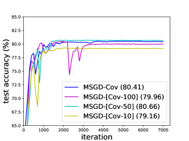
Refer to caption Refer to caption
(a) Small FashionMNIST (b) SVHN
Figure 3: The generalization of MSGD. X-axis: number of iterations; y-axis: test accuracy. (a): We randomly draw 1,00010001,000 samples from FashionMNIST as the training set, then train a small convolutional network with them. (b): We use 25,0002500025,000 samples from SVHN as the training set, then train a VGG-11 without Batch Normalization. MSGD-Cov: MSGD with Gaussian gradient noise whose covariance is the SGD covariance. MSGD-[Cov-𝐁𝐁\mathbf{B}]: MSGD-Cov with the SGD covariance estimated using a mini-batch of samples in size B𝐵B.

VGG-11

Figure 4 repeats our experiments in main text on VGG-11. The results are consistent with our main conclusions.
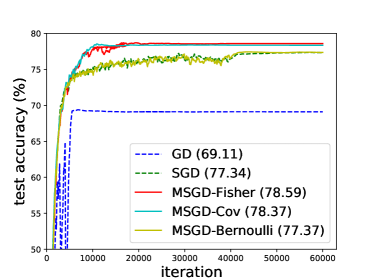
Refer to caption Refer to caption
(a) CIFAR-10, VGG-11 (b) CIFAR-10, VGG-11
Figure 4: The generalization of MSGD and mini-batch MSGD. X-axis: number of iterations; y-axis: test accuracy. (a) (b): We train a VGG-11 on CIFAR-10 without using Batch Normalization, data augmentation and weight decay. MSGD-Fisher: MSGD with Gaussian gradient noise whose covariance is the scaled Fisher. MSGD-Cov: MSGD with Gaussian gradient noise whose covariance is the SGD covariance. MSGD-Bernoulli: MSGD with Bernoulli sampling noise. SGD-𝐁𝐁\mathbf{B}: SGD with batch size B𝐵B. [MSGD-Fisher]-𝐁𝐁\mathbf{B}: mini-batch MSGD with batch size B𝐵B, and an compensatory gradient noise whose covariance is the estimated Fisher. textbf[MSGD-Cov]-𝐁𝐁\mathbf{B}: mini-batch MSGD with batch size B𝐵B, and an compensatory gradient noise whose covariance is the estimated SGD covariance.

CIFAR-100

Table 1 show addtional result for CIFAR-100 on ResNet-18. The setups follow Figure 2 (c), except that the dataset is CIFAR-100 instead of CIFAR-10.

Table 1: Additioal experimetns for CIFAR-100 on ResNet-18
Algorithm Test Accuracy
SGD-500 76.38%percent76.3876.38\%
SGD-2k 72.78%percent72.7872.78\%
[MSGD-Fisher]-2k 76.83%percent76.8376.83\%
SGD-5k 59.16%percent59.1659.16\%
[MSGD-Fisher]-5k 76.46%percent76.4676.46\%