$B$ anomalies in the nonminimal universal extra dimension model

Abstract

We investigate the $B$ anomalies in the framework of the nonminimal universal extra dimension models. Newly measured polarization parameters in $B\to D^{(*)}\tau\nu$, $P_{\tau}(D^{(*)})$ and $F_{L}(D^{*})$ as well as the ratios $R(D^{(*)})$ are considered altogether. The Kaluza-Klein modes of the $W$-boson and charged scalar contributes as the new physics effects. We find that the model parameters fit the global data very well with the minimum $\chi^{2}/{\rm d.o.f.}$ near unity, rendering $B_{c}\to\tau\nu$ branching ratios to be a few percents. The best-fit values of $R(D)$ and $R(D^{*})$ are still far from ($\gtrsim 2\sigma$) the standard model predictions.

I Introduction

The standard model (SM) of particle physics has been up to now very successful to explain many phenomena in our universe. The last missing piece of the SM, the Higgs particle was finally discovered in 2012. But there must be some new physics (NP) beyond the SM. Flavor physics is a good testing ground for the NP. Recently, some anomalies are reported in $b\to c$ semileptonic decays. The fraction of the branching ratios

$$R(D^{(*)})\equiv\frac{{\rm Br}(B\to D^{(*)}\tau\nu)}{{\rm Br}(B\to D^{(*)}\ell\nu)}~{},$$ (1)

reveals an excess over the SM predictions Amhis ,

$$R(D)_{\rm SM} = 0.299\pm 0.003~{},$$

$$R(D^{*})_{\rm SM} = 0.258\pm 0.005~{}.$$ (2)

Experiments including BABAR, Belle, and LHCb have reported somewhat larger values of $R(D^{(*)})$ than those of Eq. (2) by about $2\sim 3\sigma$ BaBar_PRL ; BaBar1 ; Belle1 ; Belle1607 ; Belle1703 ; Belle1612 ; Belle1709 ; Belle1904 ; LHCb1 ; LHCb2 . Recently the Belle collaboration announced new results Belle1904

$$R(D)_{\rm Belle1904} = 0.307\pm 0.037\pm 0.016~{},$$

$$R(D^{*})_{\rm Belle1904} = 0.283\pm 0.018\pm 0.014~{},$$ (3)

which are rather closer to Eq. (2) than the previous data and consistent with the SM within $1.2\sigma$. Combined results for all data by the heavy flavor averaging group (HFLAV) collaboration HFAG2019

$$R(D)_{\rm HFLAV} = 0.340\pm 0.027\pm 0.013~{},$$

$$R(D^{*})_{\rm HFLAV} = 0.295\pm 0.011\pm 0.008~{},$$ (4)

give a discrepancy between the SM predictions and experimental data at $3.08\sigma$ level. The BABAR measurements BaBar_PRL ; BaBar1 exclude at the 99.8% confidence level the type-II two-Higgs-doublet model (2HDM) where a charged Higgs boson contributes to $R(D^{(*)})$, while the Belle measurements Belle1 are compatible with the type-II 2HDM. It was shown that an anomalous $\tau$ coupling to the charged Higgs in the 2HDM can explain the data very well jplee . In extra dimension models the overlapping between the wave functions of $\tau$ and the neutral scalar could be weak to make $\tau$ screened from the scalar vacuum, resulting in an enhancement of $\tau$ couplings to charged Higgs. For discussions in the 2HDM, see Refs. Andreas ; Fazio ; Cline ; Koerner ; Chen ; Iguro . There are many other NP scenarios to explain the $R(D^{(*)})$ anomaly, including leptoquark models Dorsner ; Alonso ; Bauer ; Barbieri ; DiLuzio ; Calibbi ; Becirevic , composite models Barbieri2 ; Buttazzo ; Bordone ; Matsuzaki , warped extra dimensions Megias1 ; Megias2 ; DAmbrosio ; Blanke0 , etc. Kang ; Huang ; Bardhan .

On top of the ratio $R(D^{(*)})$ the Belle collaboration measured the relevant polarizations in $B\to D^{(*)}\tau\nu$ decays. One can consider observable parameters associated with $D^{*}$ as well as $\tau$. The $\tau$-polarization asymmetry is defined as

$$P_{\tau}(D^{(*)})\equiv\frac{\Gamma^{D^{(*)}}_{\tau}(+)-\Gamma^{D^{(*)}}_{\tau}(-)}{\Gamma^{D^{(*)}}_{\tau}(+)+\Gamma^{D^{(*)}}_{\tau}(-)}~{},$$ (5)

where $\Gamma^{D^{(*)}}_{\tau}(\pm)$ is the decay width for $(\pm)~{}\tau$ helicity. The SM predictions are Tanaka2010 ; Tanaka2012

$$P_{\tau}(D)_{\rm SM}=0.325\pm 0.009~{},~{}~{}~{}P_{\tau}(D^{*})_{\rm SM}=-0.497\pm 0.013~{}.$$ (6)

The experimental result is Belle1612 ; Belle1709

$$P_{\tau}(D^{*})=-0.38\pm 0.51^{+0.21}_{-0.16}~{}.$$ (7)

The longitudinal $D^{*}$ polarization is

$$F_{L}(D^{*})\equiv\frac{\Gamma(B\to D^{*}_{L}\tau\nu)}{\Gamma(B\to D^{*}\tau\nu)}~{},$$ (8)

where the Belle’s measurement is Abdesselam

$$F_{L}(D^{*})=0.60\pm 0.08\pm 0.035~{},$$ (9)

while the SM value is estimated to be Alok2016

$$F_{L}(D^{*})_{\rm SM}=0.46\pm 0.04~{}.$$ (10)

The polarization parameters could provide more information about the Lorentz structure of possible NP.

In this paper we consider the nonminimal universal extra dimension (nmUED) model Cheng ; Aguila0301 ; Aguila0302 ; Flacke08 ; Datta1205 ; Datta1408 ; Datta16 ; Datta17 to fit the global data on $R(D^{(*)})$ and polarization parameters. In the universal extra dimension (UED) models there is an extra spacelike dimension with a flat metric compactified on an $S^{1}/Z_{2}$ orbifold, where the SM particles could reside. Each SM particles is accompanied by infinite towers of Kaluza-Klein (KK) states. There are two branes at the endpoints of the orbifold. The reflection symmetry of the bulk space provides with the KK-parity conservation. The lightest KK particle is a natural candidate for dark matter, which makes the UED scenario a strong alternative to the SM. As discussed in Biswas , in the minimal version of the UED (MUED) there are no new couplings at the tree level relevant to $R(D^{(*)})$. The radiative corrections include bulk corrections and boundary localized ones. In the MUED models the latter is adjusted to cancel the cutoff dependent corrections. The nmUED models allow the boundary localized terms (BLTs) to be free parameters. In this analysis we include the BLTs with free strength parameters. The presence of BLTs changes mass spectrum and couplings of KK modes of the UED model. The NP effects enter through the possible interactions between a pair of zero-mode fermion and even KK-modes of charged gauge boson or scalar, associated with the BLTs Biswas ; Dasgupta . These kinds of interactions are not allowed in the MUED because of the KK-wave function orthogonality. Since the new interactions contribute to $R(D^{(*)})$ at the tree level, we expect the nmUED model would provide some hints to solve the $R(D^{(*)})$ puzzle.

The paper is organized as follows. In the next section the nmUED model is introduced. Section III provides the various observables in numerical forms. The results and discussions are given in Sec. IV, and we conclude in Sec. V.

II nmUED model

We assume that there is one flat extra dimension ($y$) compactified on an $S^{1}/Z_{2}$ orbifold with radius $R$. Two branes are located at the endpoints $y=0$ and $y=\pi R$ where both boundary terms are equal. The 5D action for fermions $f$ is Biswas

$${\cal S}_{f} = \sum_{f=q,\ell}\int d^{4}x\int_{0}^{\pi R}dy\left\{i{\bar{\Psi}}^{f}_{L}\Gamma^{M}{\cal D}_{M}\Psi^{f}_{L}+r_{f}\left[\delta(y)+\delta(y-\pi R)\right]i{\bar{\Psi}}^{f}_{L}\gamma^{\mu}{\cal D}_{\mu}P_{L}\Psi^{f}_{L}\right.$$ (11)

$$\left.+i{\bar{\Psi}}^{f}_{R}\Gamma^{M}{\cal D}_{M}\Psi^{f}_{R}+r_{f}\left[\delta(y)+\delta(y-\pi R)\right]i{\bar{\Psi}}_{R}\gamma^{\mu}{\cal D}_{\mu}P_{R}\Psi^{f}_{R}\right\}~{},$$

where $\Psi^{f}_{L,R}(x,y)$ are the 5D four component Dirac spinors for fermions $f=q,\ell$. In terms of two component spinors,

$$\Psi^{f}_{L,R}(x,y)=\begin{pmatrix}\psi^{f}_{L,R}(x,y)\\ \chi^{f}_{L,R}(x,y)\end{pmatrix}=\sum_{n}\begin{pmatrix}\psi^{f(n)}_{L,R}(x)F^{f(n)}_{L,R}(y)\\ \chi^{f(n)}_{L,R}(x)G^{f(n)}_{L,R}(y)\end{pmatrix}~{},$$ (12)

where $F^{f(n)}_{L,R}(y)$ and $G^{f(n)}_{L,R}(y)$ are the $n$-th KK-wave functions. In Eq. (11) $r_{f}$ is the strength of the boundary localized terms. They are related to the mass of the $n$th KK-excitation $m_{f^{(n)}}$ by the transcendental equation

$$\frac{r_{f}m_{f^{(n)}}}{2}=\left\{\begin{array}[]{cc}-\tan\left(\frac{m_{f^{(n)}}\pi R}{2}\right)~{}\text{for even}~{}n\\ \cot\left(\frac{m_{f^{(n)}}\pi R}{2}\right)~{}\text{for odd}~{}n\end{array}\right.~{}.$$ (13)

As for the gauge boson sector, the 5D action is

$${\cal S}_{\rm gauge} = -\frac{1}{4}\int d^{4}x\int_{0}^{\pi R}dy\left\{W^{i}_{MN}W^{iMN}+r_{V}\left[\delta(y)+\delta(y-\pi R)\right]W^{i}_{\mu\nu}W^{i\mu\nu}\right.$$ (14)

$$\left.+B_{MN}B^{MN}+r_{V}\left[\delta(y)+\delta(y-\pi R)\right]B_{\mu\nu}B^{\mu\nu}\right\}~{},$$

where $W^{i}_{MN}$, $B_{MN}$ are the 5D gauge field strength tensors. The $n$th KK-mass of the gauge boson is

$$M_{W^{(n)}}=\sqrt{M_{W}^{2}+m_{V^{(n)}}^{2}}~{},$$ (15)

where $m_{V^{(n)}}$ satisfies the same transcendental equation as Eq. (13). For the $5D$ scalar field $\Phi(x,y)$, the action is

$${\cal S}_{\phi}=\int d^{4}x\int_{0}^{\pi R}dy\left\{\left({\cal D}_{M}\Phi\right)^{\dagger}\left({\cal D}^{M}\Phi\right)+r_{\phi}\left[\delta(y)+\delta(y-\pi R)\right]\left({\cal D}_{\mu}\Phi\right)^{\dagger}\left({\cal D}^{\mu}\Phi\right)\right\}~{}.$$ (16)

We choose $r_{\phi}=r_{V}$ for proper gauge fixing Jha , and consequently the mass of the KK-scalar is $m_{\phi^{(n)}}=m_{V^{(n)}}$. The Yukawa interaction is described by

$${\cal S}_{Y}=-\sum_{f}\int d^{4}x\int_{0}^{\pi R}dy\left\{\lambda_{5}{\bar{\Psi}}^{f}_{L}{\tilde{\Phi}}\Psi^{f}_{R}+r_{Y}\left[\delta(y)+\delta(y-\pi R)\right]\lambda_{5}{\bar{\psi}^{f}}_{L}{\tilde{\Phi}}\chi^{f}_{R}+{\rm H.c.}\right\}~{},$$ (17)

where $\lambda_{5}$ is the $5D$ Yukawa coupling and $r_{Y}$ is the boundary strength.

In nmUED, new KK particles contribute to $B$ decays. As mentioned in Sec. I even KK-modes of $W$-boson as well as charged Higgs couple to a pair of zero-mode fermions, which provide new vector and scalar interactions respectively. The effects are encoded in the overlap integrals

$$I_{n}^{fg} = \sqrt{\pi R\left(1+\frac{r_{V}}{\pi R}\right)}\int_{0}^{\pi R}dy\Big{\{}1+r_{f}\left[\delta(y)+\delta(y-\pi R)\right]\Big{\}}a^{n}F_{L}^{f(0)}F_{L}^{f(0)}~{},$$ (18)

$$I_{n}^{fY} = \sqrt{\pi R\left(1+\frac{r_{V}}{\pi R}\right)}\int_{0}^{\pi R}dy\Big{\{}1+r_{Y}\left[\delta(y)+\delta(y-\pi R)\right]\Big{\}}f^{n}F_{L}^{f(0)}G_{R}^{f(0)}~{},$$

where $a^{n}$ and $h^{n}$ are $n$th KK-mode of the $W$-boson and scalar, respectively. For $r_{\phi}=r_{V}$, $a^{n}=h^{n}$, and further if $r_{f}=r_{Y}$ then Biswas

$$I_{n}^{fg}=I_{n}^{fY}\equiv I_{n}^{f}=\frac{\sqrt{2}({\hat{r}}_{f}-{\hat{r}}_{V})\sqrt{1+{\hat{r}}_{V}}}{(1+{\hat{r}}_{f})\sqrt{1+r_{V}^{2}m_{V^{(n)}}^{2}/4+{\hat{r}}_{V}}}~{},$$ (19)

where ${\hat{r}}\equiv r/(\pi R)$. Actually, $I_{n}^{f}$ is the interaction term between a pair of zero-mode fermion $f$ and $n$th KK-modes of $W$-boson or scalar, which encodes the NP effects on observables.

III Observables

Now the effective Hamiltonian for $b\to c\ell\nu$ is

$${\cal H}_{\rm eff}=\frac{4G_{F}}{\sqrt{2}}V_{cb}\sum_{\ell=\mu,\tau}\left\{(1+C_{V}^{\ell}){\cal O}_{V}^{\ell}+C_{S}^{\ell}{\cal O}_{S}^{\ell}\right\}~{},$$ (20)

where the operators ${\cal O}_{V,S}^{\ell}$ are defined by

$${\cal O}_{V}^{\ell} = \left({\bar{c}}_{L}\gamma^{\mu}b_{L}\right)\left({\bar{\ell}}_{L}\gamma_{\mu}\nu_{\ell L}\right)~{},$$ (21)

$${\cal O}_{S}^{\ell} = \left({\bar{c}}_{L}b_{R}\right)\left({\bar{\ell}}_{R}\nu_{\ell L}\right)~{}.$$ (22)

The NP effects are encapsulated in the Wilson coefficients $C_{V,S}^{\ell}$ given as Biswas

$$C_{V}^{\ell} = \sum_{n\geq 2}\left[\frac{M_{W}^{2}}{M_{W^{(n)}}^{2}}\right]I_{n}^{q}I_{n}^{\ell}~{},$$ (23)

$$C_{S}^{\ell} = \sum_{n\geq 2}\left[\frac{m_{b}m_{\ell}}{M_{W^{(n)}}^{2}}\right]\left[\frac{M_{W}^{2}}{M_{W^{(n)}}^{2}}\right]\left\{\cos\left(\frac{1}{2}\tan^{-1}\left[\frac{m_{c}}{m_{f^{(n)}}}\right]-\frac{1}{2}\tan^{-1}\left[\frac{m_{\ell}}{m_{f^{(n)}}}\right]\right)\right.$$ (24)

$$-\left.\sin\left(\frac{1}{2}\tan^{-1}\left[\frac{m_{c}}{m_{f^{(n)}}}\right]+\frac{1}{2}\tan^{-1}\left[\frac{m_{\ell}}{m_{f^{(n)}}}\right]\right)\right\}I_{n}^{q}I_{n}^{\ell}~{}.$$

From ${\cal H}_{\rm eff}$ one can calculate the transition amplitudes and decay rates for $B\to D^{(*)}$ decays, and construct various observable parameters. We only concentrate on the numerical results for the observables in our analysis. Numerically the observables for $B\to D^{(*)}\ell\nu_{\ell}$ decays are (at $\mu=m_{b}$ scale) Blanke

$$R(D) = 2R_{\rm SM}(D)\frac{\left(1+C_{V}^{\tau}\right)^{2}+1.54\left(1+C_{V}^{\tau}\right)C_{S}^{\tau}+1.09\left(C_{S}^{\tau}\right)^{2}}{1+\left(1+C_{V}^{\mu}\right)^{2}+1.54\left(1+C_{V}^{\mu}\right)C_{S}^{\mu}+1.09\left(C_{S}^{\mu}\right)^{2}}~{},$$ (25)

$$R(D^{*}) = 2R_{\rm SM}(D^{*})\frac{\left(1+C_{V}^{\tau}\right)^{2}+0.13\left(1+C_{V}^{\tau}\right)C_{S}^{\tau}+0.05\left(C_{S}^{\tau}\right)^{2}}{1+\left(1+C_{V}^{\mu}\right)^{2}+0.13\left(1+C_{V}^{\mu}\right)C_{S}^{\mu}+0.05\left(C_{S}^{\mu}\right)^{2}}~{},$$ (26)

$$P_{\tau}(D) = \frac{0.32\left(1+C_{V}^{\tau}\right)^{2}+1.54\left(1+C_{V}^{\tau}\right)C_{S}^{\tau}+1.09\left(C_{S}^{\tau}\right)^{2}}{\left(1+C_{V}^{\tau}\right)^{2}+1.54\left(1+C_{V}^{\tau}\right)C_{S}^{\tau}+1.09\left(C_{S}^{\tau}\right)^{2}}~{},$$ (27)

$$P_{\tau}(D^{*}) = \frac{-0.49\left(1+C_{V}^{\tau}\right)^{2}+0.13\left(1+C_{V}^{\tau}\right)C_{S}^{\tau}+0.05\left(C_{S}^{\tau}\right)^{2}}{\left(1+C_{V}^{\tau}\right)^{2}+0.13\left(1+C_{V}^{\tau}\right)C_{S}^{\tau}+0.05\left(C_{S}^{\tau}\right)^{2}}~{},$$ (28)

$$F_{L}(D^{*}) = \frac{0.46\left(1+C_{V}^{\tau}\right)^{2}+0.13\left(1+C_{V}^{\tau}\right)C_{S}^{\tau}+0.05\left(C_{S}^{\tau}\right)^{2}}{\left(1+C_{V}^{\tau}\right)^{2}+0.13\left(1+C_{V}^{\tau}\right)C_{S}^{\tau}+0.05\left(C_{S}^{\tau}\right)^{2}}~{},$$ (29)

$${\rm Br}(B_{c}\to\tau\nu) = 0.02\left(\frac{f_{B_{c}}}{0.43~{}{\rm GeV}}\right)\Big{[}1+C_{V}^{\tau}+4.3C_{S}^{\tau}\Big{]}^{2}~{}.$$ (30)

The results are obtained from the numerical values of the relevant form factors of $B\to D$ Aoki and $B\to D^{*}$ transitions Amhis ; Bernlochner .

The branching ratio of $B_{c}\to\tau\nu$, ${\rm Br}(B_{c}\to\tau\nu)$ could impose strong constraints on $R(D^{(*)})$ Alonso2016 . Since ${\rm Br}(B_{c}\to\tau\nu)\sim\left(1+C_{V}^{\tau}+4.3C_{S}^{\tau}\right)^{2}$, the branching ratio directly affects the relevant Wilson coefficients. There are still debates on the upper bound of ${\rm Br}(B_{c}\to\tau\nu)$. The strongest bound is from Ref. Akeroyd where ${\rm Br}(B_{c}\to\tau\nu)<10\%$. On the other hand, Ref. Blanke argues that the branching ratio could be as large as $60\%$. In this analysis we do not explicitly impose the ${\rm Br}(B_{c}\to\tau\nu)$ constraints, because as we will see later our results are compatible with small values of ${\rm Br}(B_{c}\to\tau\nu)$. The experimental data for various observables used in this analysis are listed in Table 1.

	$R(D)$	$R(D^{*})$
BABAR	$0.440\pm 0.058\pm 0.042$	$0.332\pm 0.024\pm 0.018$ BaBar1
Belle(2015)	$0.375\pm 0.064\pm 0.026$	$0.293\pm 0.038\pm 0.015$ Belle1
Belle(2016)	$-$	$0.302\pm 0.030\pm 0.011$ Belle1607
Belle(2017)	$-$	$0.276\pm 0.034^{+0.029}_{-0.026}$ Belle1703
Belle(2017)	$-$	$0.270\pm 0.035^{+0.028}_{-0.025}$ Belle1612 ; Belle1709
Belle(2019)	$0.307\pm 0.037\pm 0.016$	$0.283\pm 0.018\pm 0.014$ Belle1904
LHCb(2015)	$-$	$0.336\pm 0.027\pm 0.030$ LHCb1
LHCb(2017)	$-$	$0.291\pm 0.019\pm 0.026\pm 0.013$ LHCb2
	$P_{\tau}(D^{*})$	$F_{L}(D^{*})$
Belle(2017)	$-0.38\pm 0.51^{+0.21}_{-0.16}$Belle1612 ; Belle1709	$-$
Belle(2019)	$-$	$0.60\pm 0.08\pm 0.04$ Abdesselam

Table 1: Experimental data for $R(D^{(*)})$, $P_{\tau}(D^{(*)})$ and $F_{L}(D^{*})$. The uncertainties are $\pm$(statistical)$\pm$(systematic). For the third uncertainty of LHCb(1711), see LHCb2 for details. For BABAR, Belle(2015), and Belle(2019) results, the correlations between $R(D)$ and $R(D^{*})$ are $-0.31$, $-0.50$ and $-0.51$ respectively HFAG2019 .

IV Results

We implement the global $\chi^{2}$ fit for the observables in Table 1. We first define the $\chi^{2}$ as

$$\chi^{2}\equiv\sum_{i,j}\left[{\cal O}_{i}^{\rm exp}-{\cal O}_{i}^{\rm th}\right]{\cal C}_{ij}^{-1}\left[{\cal O}_{j}^{\rm exp}-{\cal O}_{j}^{\rm th}\right]~{},$$ (31)

where ${\cal O}_{i}^{\rm exp}$ are the experimental data while ${\cal O}_{i}^{\rm th}$ are the theoretical predictions of Eqs.(25)-(30), and ${\cal C}_{ij}$ are the correlation matrix elements.

There are two major constraints. One is from the oblique parameters of the electroweak precision test (EWPT) Flacke2012 ; Flacke2013 ; Datta2013 ; Dey . In the nmUED model, the Fermi constant is modified by the tree level contributions of even $n$th KK-modes of $W$-bosons to the four-fermion interactions. This kind of correction is absent in the MUED scenario. The Fermi constant in nmUED is now written as

$$G_{F}=G_{F}^{0}+\delta G_{F}~{}.$$ (32)

Here $G_{F}^{0}$ is the Fermi constant in the SM and $\delta G_{F}$ is the correction from the new contributions of $W^{\pm}$ KK-modes. Explicitly Biswas ,

$$G_{F}^{0}=\frac{g^{2}}{4\sqrt{2}M_{W}^{2}}~{},~{}~{}~{}\delta G_{F}=\sum_{n\geq 2}\frac{g^{2}(I_{n}^{\ell})^{2}}{4\sqrt{2}m_{W^{(n)}}^{2}}~{},$$ (33)

where $g$ is the gauge coupling constant. Note that $\delta G_{F}\sim(I_{n}^{\ell})^{2}$ because the Fermi constant is derived from the muon lifetime. We only consider the 2nd KK contributions for simplicity. Now the Fermi constant is related to the Peskin-Tacheuchi parameters as Flacke2012

$$S_{\rm nmUED}=0~{},~{}~{}~{}T_{\rm nmUED}=-\frac{1}{\alpha}\frac{\delta G_{F}}{G_{F}}~{},~{}~{}~{}U_{\rm nmUED}=\frac{4\sin^{2}\theta_{W}}{\alpha}\frac{\delta G_{F}}{G_{F}}~{},$$ (34)

where we neglect possible loop effects which are subdominant compared to the tree-level contributions to $\delta G_{F}$. We use the data Gfitter

$$S=0.05\pm 0.11~{},~{}~{}~{}T=0.09\pm 0.13~{},~{}~{}~{}U=0.01\pm 0.11~{},$$ (35)

where the correlation coefficients are

$$\rho_{ST}=0.90~{},~{}~{}~{}\rho_{TU}=-0.83~{},~{}~{}~{}\rho_{US}=-0.59~{}.$$ (36)

Following the methods of Dey , we impose the $S$, $T$, $U$ constraints by requiring $\chi_{STU}^{2}<6.18$ at $2\sigma$ where $\chi_{STU}^{2}$ is defined by the covariant matrix relevant for the $S$, $T$, $U$ parameters, similarly to Eq. (31).

The other major constraint comes from the LHC dilepton resonance searches. At the LHC the second KK gauge boson $A^{(2)}$ can be produced via the KK number violating interactions, subsequently decaying into the SM particles. Recent results from ATLAS dilepton resonance searches at the 13 TeV with $13.3~{}{\rm fb}^{-1}$ provide a stringent constraint on the nmUED parameters Flacke2017 . We reflect the results of Flacke2017 on the strength of the BLKT in the gauge sector to constrain our analysis to the region $0\leq r_{V}/R\leq 0.5$. The best-fit values for the minimum $\chi^{2}$ are listed in Table 2.

$R(D)$	$R(D^{*})$	$P_{\tau}(D)$	$P_{\tau}(D^{*})$	$F_{L}(D^{*})$	${\rm Br}(B_{c}\to\tau\nu)$	$\chi^{2}_{\rm min}/{\rm d.o.f.}$
$0.343$	$0.296$	$0.320$	$-0.490$	$0.460$	$2.75\times 10^{-2}$	$1.25$

Table 2: Best-fit values.

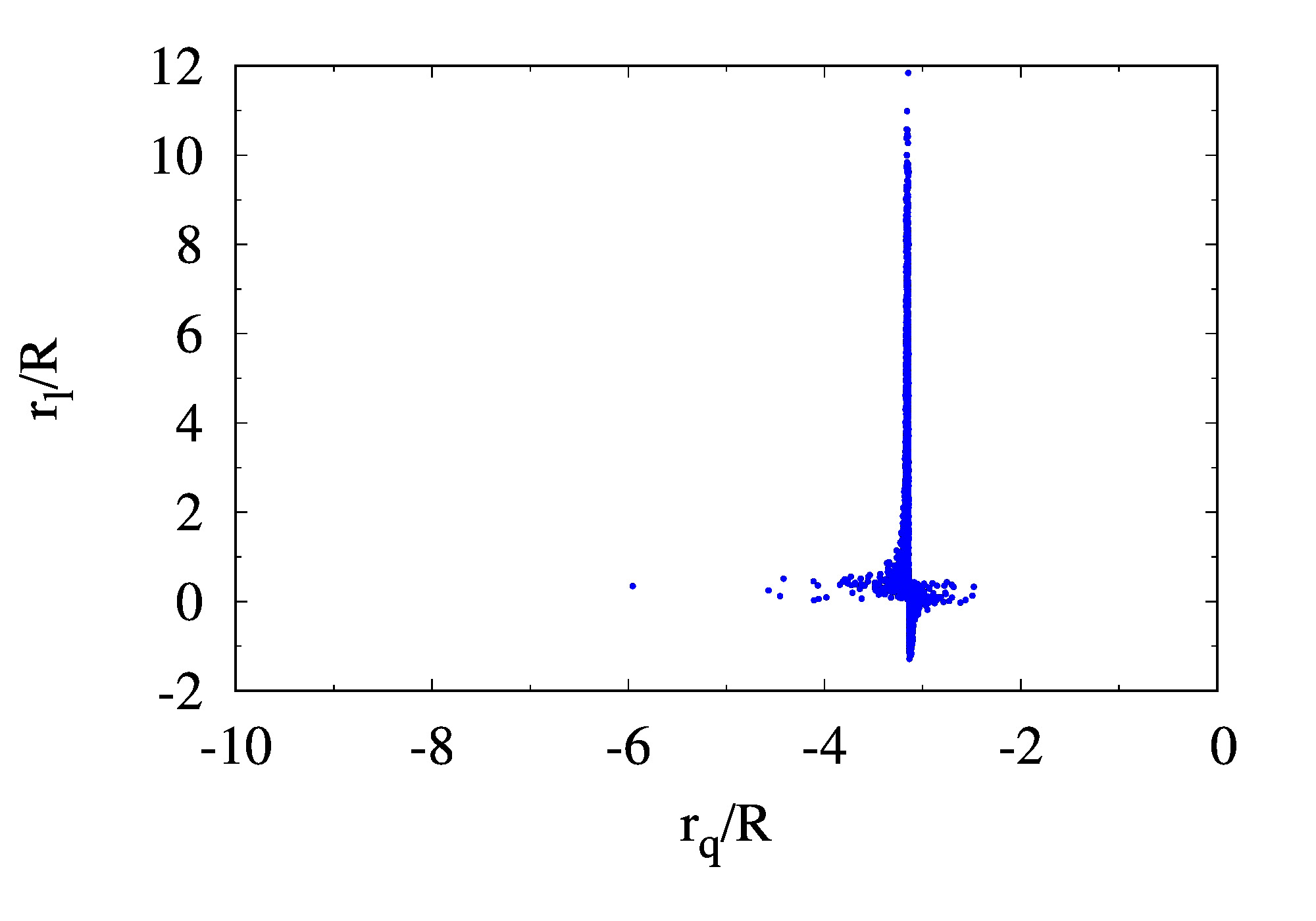
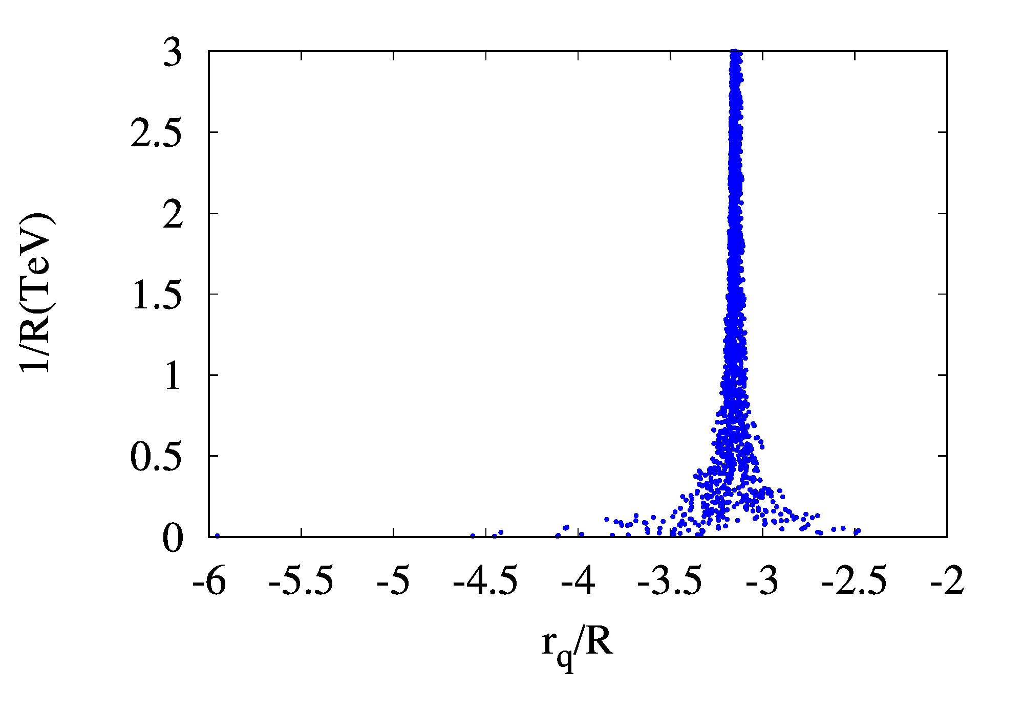
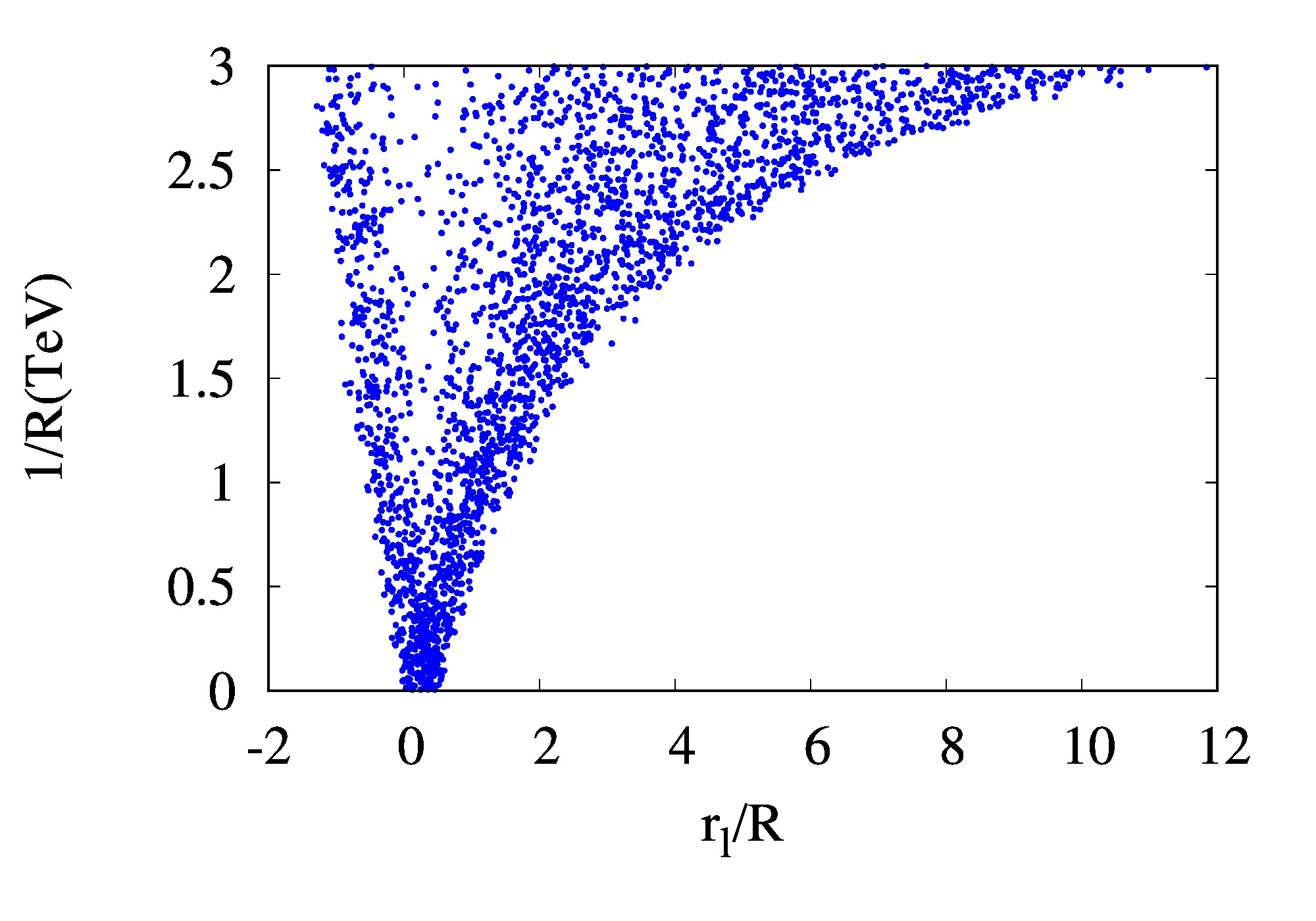
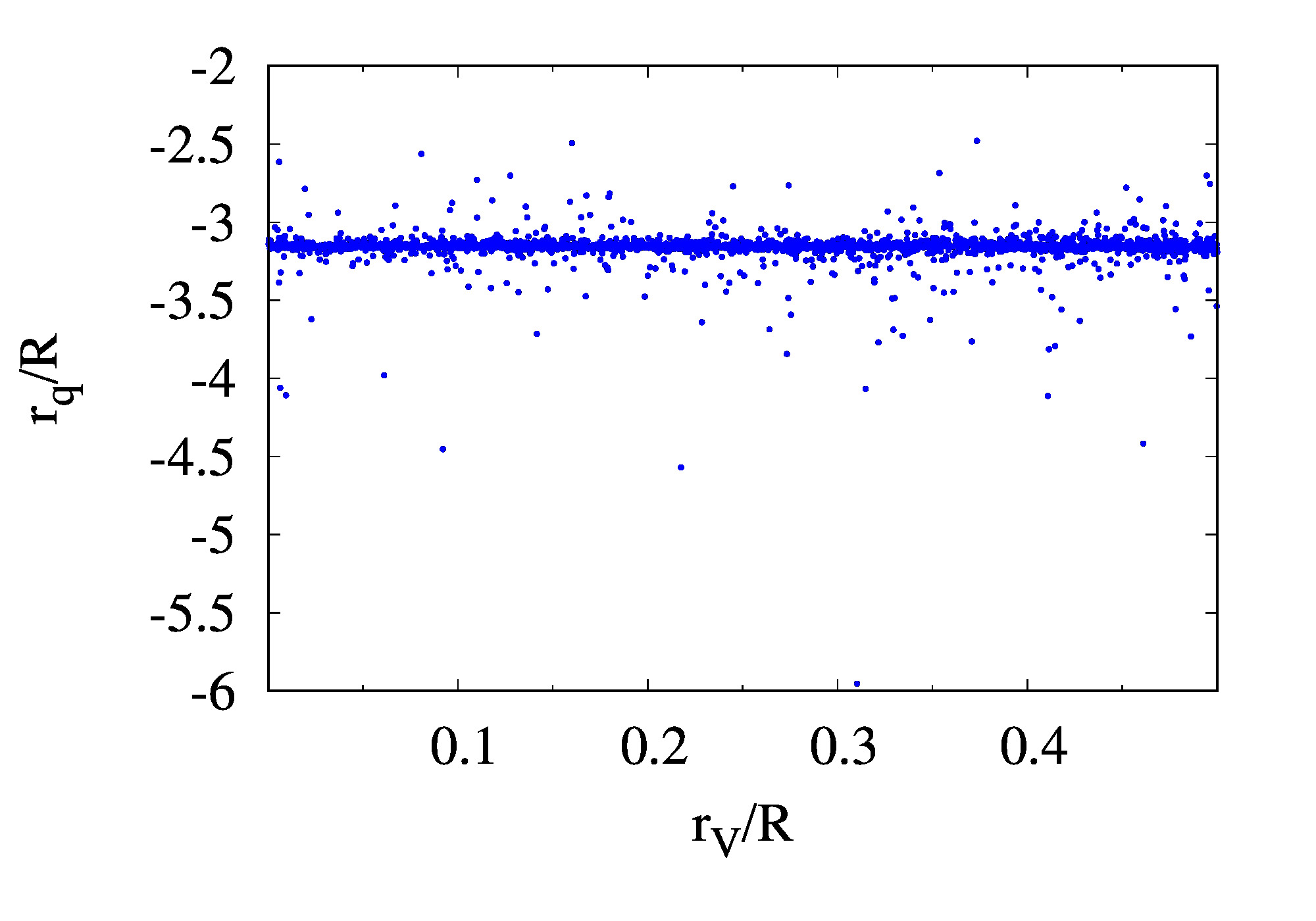
In Fig. 1, we plot the allowed regions of the nmUED parameters at the $2\sigma$ level. We scanned over the range $0\leq 1/R\leq 3~{}{\rm TeV}$.

(a)	(b)
(c)	(d)

Figure 1: Allowed regions of model parameters of nmUED at the $2\sigma$ level.

A noticeable feature is that the allowed range of $r_{q}/R$ is rather narrow with negative values, contrary to that of $r_{\ell}/R$ as shown in Fig. 1 (a). In the nmUED models, $r_{q,\ell}$ are considered as free parameters and can be negative but with some restrictions. The fields $F_{L,R}^{f(n)}$ and $G_{L,R}^{f(n)}$ of Eq. (12) have normalization factor Datta16 ; Datta17 ; Biswas ,

$$N_{n}^{f}=\sqrt{\frac{2}{\pi R}}\frac{1}{\sqrt{1+r_{f}^{2}m_{f^{(n)}}^{2}/4+r_{f}/(\pi R)}}~{}.$$ (37)

For $N_{n}^{f}$ to be meaningful, $r_{f}/(\pi R)>-1-r_{f}^{2}m_{f^{(n)}}^{2}/4$ and for small values of $r_{f}m_{f^{(n)}}$, $r_{f}/R\gtrsim-\pi$. Our results of Fig. 1 satisfy this requirement. Note that the points near $r_{q}/R=-\pi$ are favorable for larger $R(D)$ and smaller $\chi^{2}$.

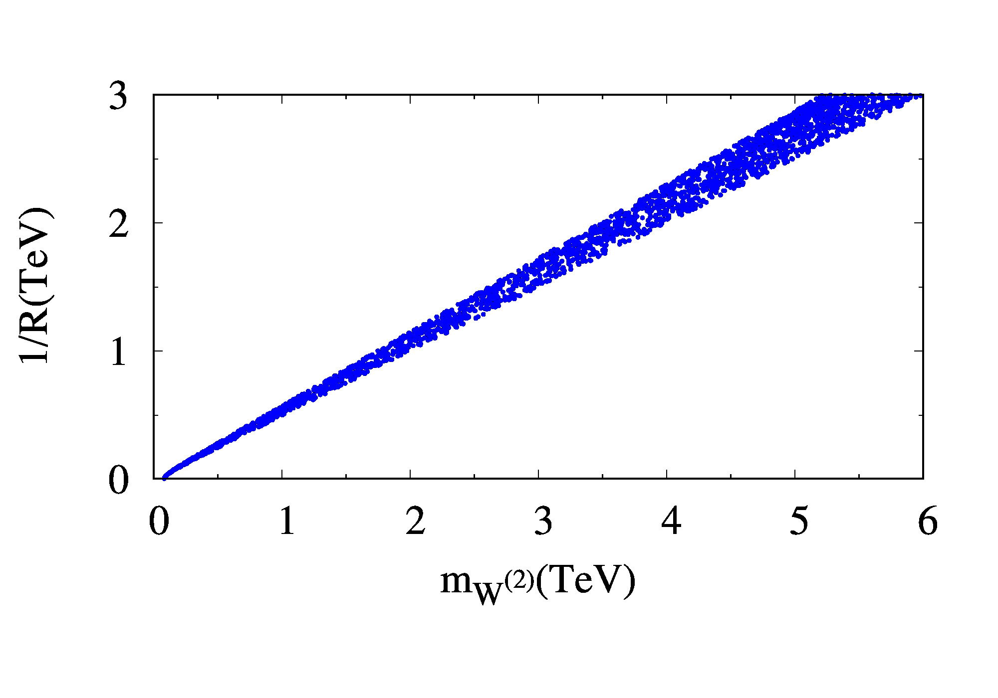
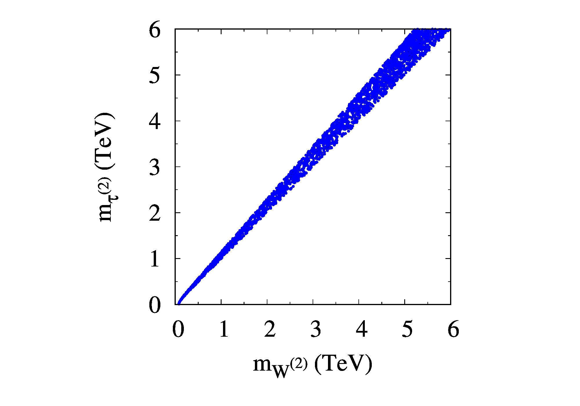
Figure 2 shows the 2nd KK masses $m_{W^{(2)}}$ and $m_{\tau^{(2)}}$.

(a)	(b)

Figure 2: Mass scales of nmUED at $2\sigma$.

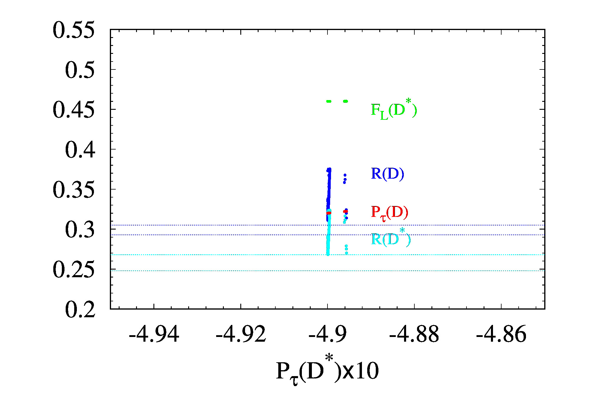
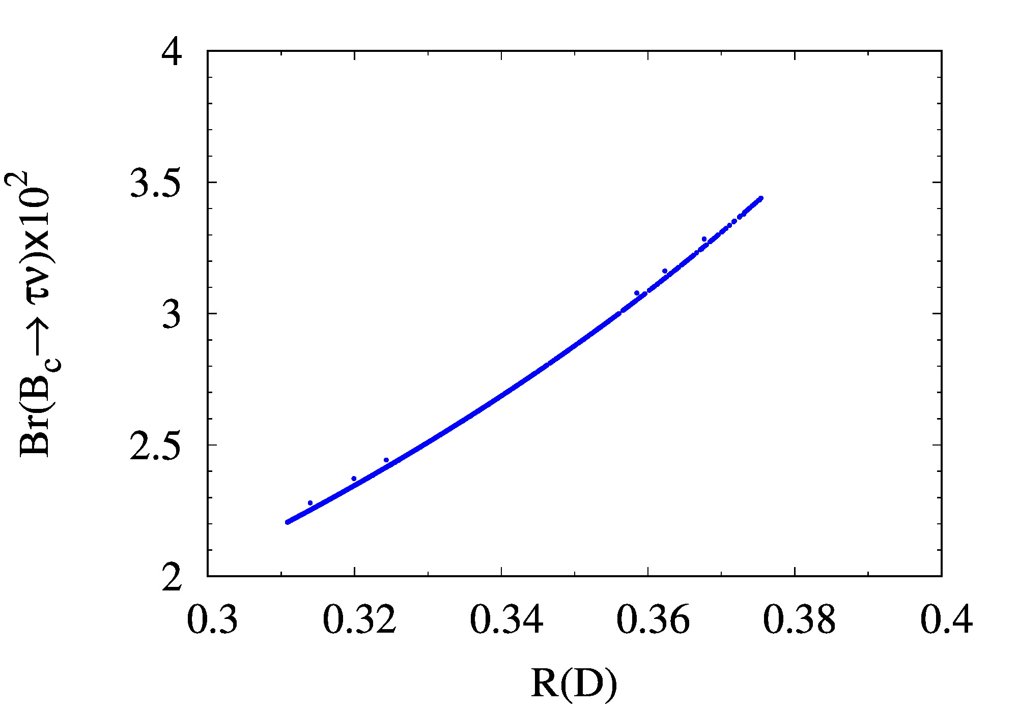
Allowed values of various observables at $2\sigma$ are given in Fig. 3.

(a)	(b)

Figure 3: Allowed values for various observables at $2\sigma$. In (a) numerical values of $R(D^{(*)})$, $P_{\tau}(D)$, and $F_{L}(D^{*})$ are plotted with respect to the values of $P_{\tau}(D^{*})$. The horizontal lines are the SM predictions at $2\sigma$ for $R(D)$ (blue) and $R(D^{*})$ (cyan). Other polarization parameters $P_{\tau}(D^{(*)})$ and $F_{L}(D^{*})$ are consistent with the SM values at $2\sigma$. In (b) the branching ratio of ${\rm Br}(B_{c}\to\tau\nu)$ vs $R(D)$ is plotted.

As can be seen in Fig. 3 (a), $R(D)$ is still far away from the SM predictions beyond $2\sigma$ level while $R(D^{*})$ values have small overlaps at the edge of the SM-allowed range within $2\sigma$ . But the best-fit values of $R(D^{(*)})$ in Table 1 are still beyond the SM by more than $2\sigma$. Other polarization observables $P_{\tau}(D^{(*)})$ and $F_{L}(D^{*})$ are consistent with the SM. Figure 3 (b) shows that the branching ratio ${\rm Br}(B_{c}\to\tau\nu)$ lies safely within a few percents.

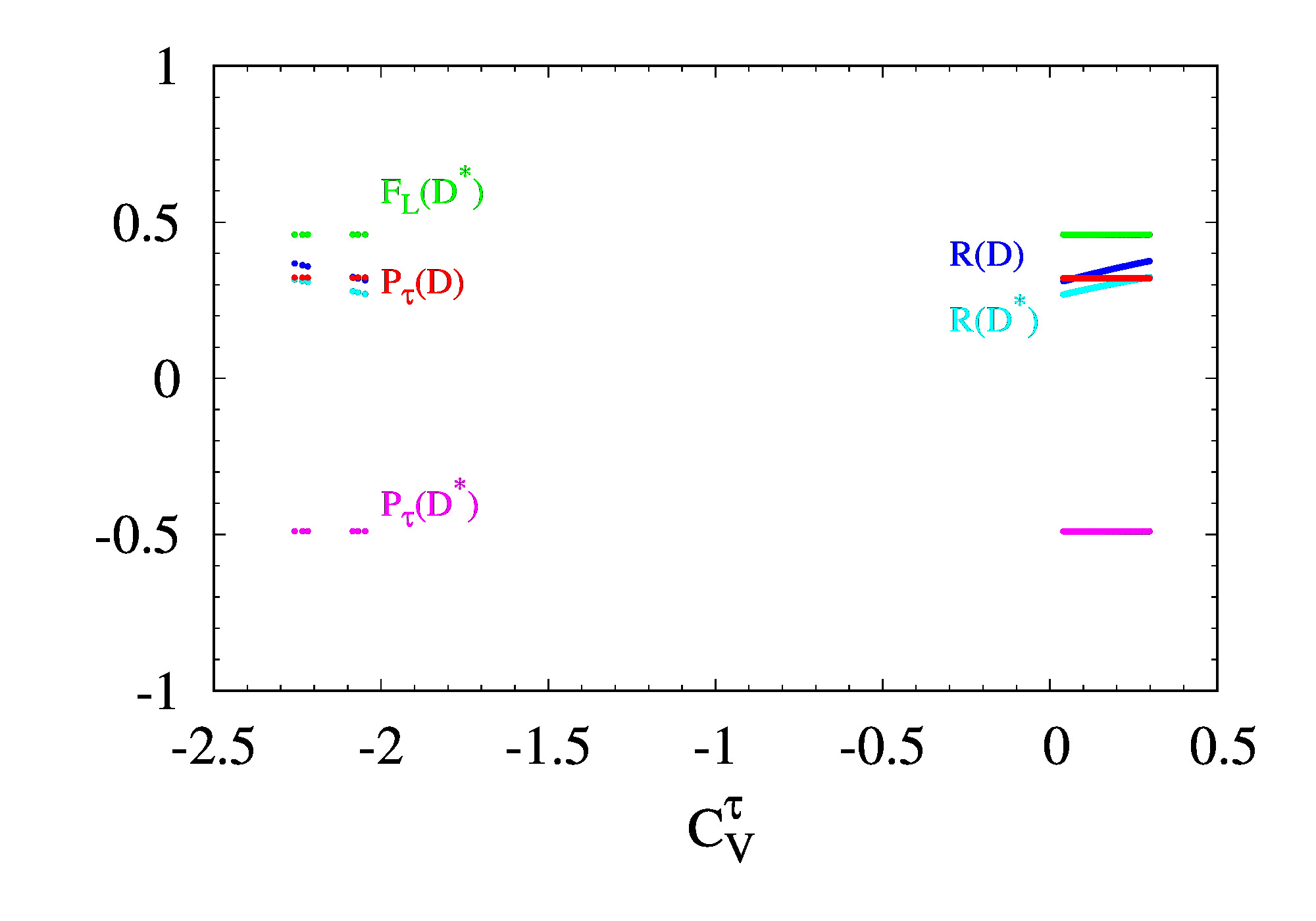
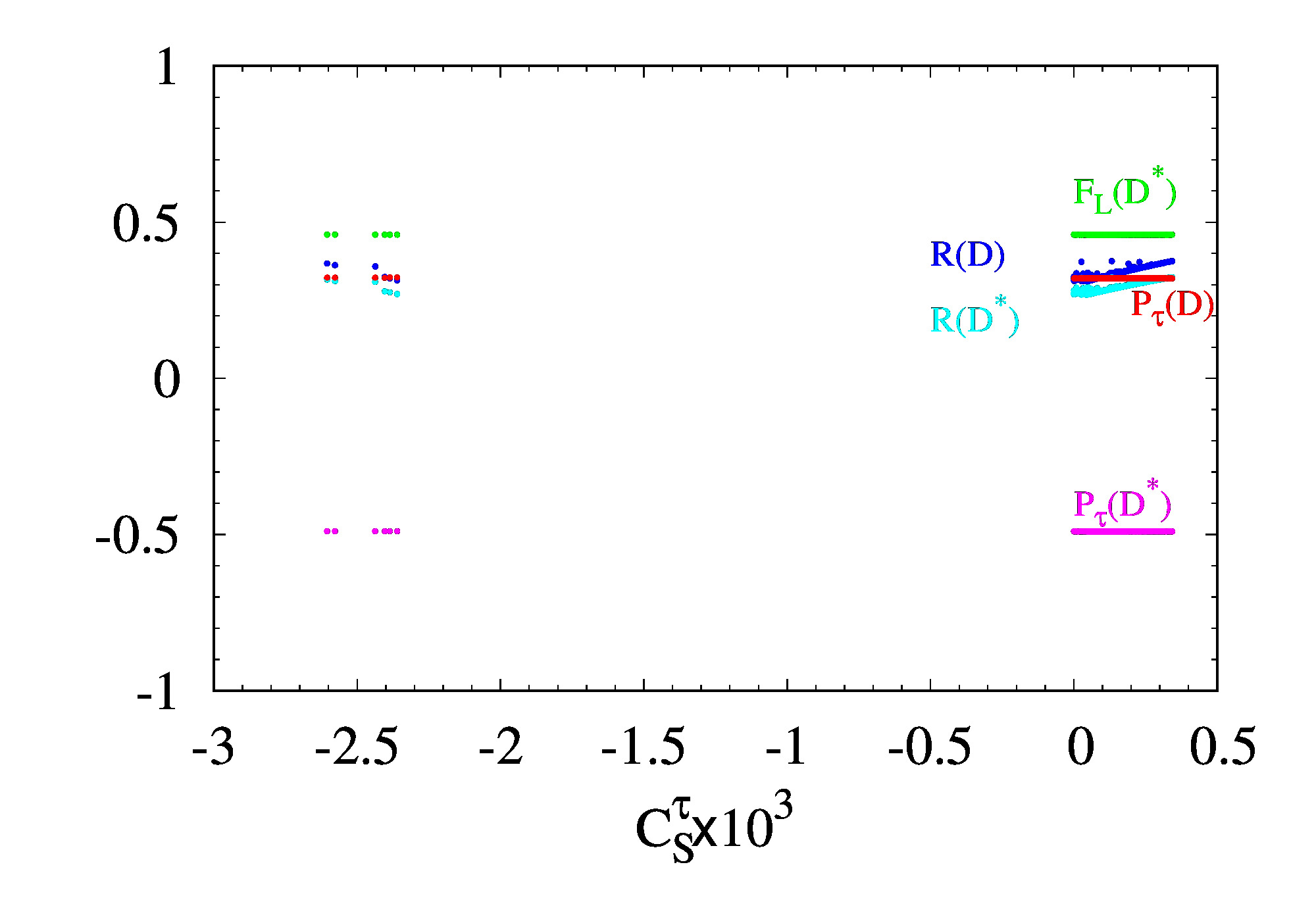
Contributions of the Wilson coefficients to observables at $2\sigma$ are depicted in Fig. 4.

(a)	(b)

Figure 4: Wilson coefficients $C_{V,S}^{\tau}$ and observables.

We find that the pattern for $C_{V}^{\mu}$ is very similar to that of $C_{S}^{\mu}$. Note that the Wilson coefficients are

$$C_{V,S}\sim I_{n}^{q}I_{n}^{\ell}~{},$$ (38)

while the EW precision parameters are

$$T_{\rm nmUED}(U_{\rm nmUED})\sim\delta G_{F}\sim\left(I_{n}^{\ell}\right)^{2}~{}.$$ (39)

In case of $r_{q}=r_{\ell}$ the overlap integrals become $I_{n}^{q}=I_{n}^{\ell}$ and $C_{V,S}\sim\left(I_{n}^{\ell}\right)^{2}$, which are directly affected by the oblique parameters of Eq. (39). According to Eq. (35) EWPT prefers small $\left(I_{n}^{\ell}\right)^{2}$. It means that for $r_{q}=r_{\ell}$ EWPT requires smaller $C_{V,S}$, which results in smaller $R(D^{(*)})$ and does not fit data so well. In other words, we find that $R(D^{(*)})$ anomalies require $r_{q}\neq r_{\ell}$ in nmUED. The situation is depicted in Fig. 5 where $R(D)$ vs $\chi^{2}/{\rm d.o.f.}$ are compared for $r_{\ell}/R=r_{q}/R$ and $r_{\ell}/R\neq r_{q}/R$ cases.

Figure 5: $R(D)$ vs $\chi^{2}/{\rm d.o.f.}$ for $r_{\ell}/R=r_{q}/R$ and $r_{\ell}/R\neq r_{q}/R$.

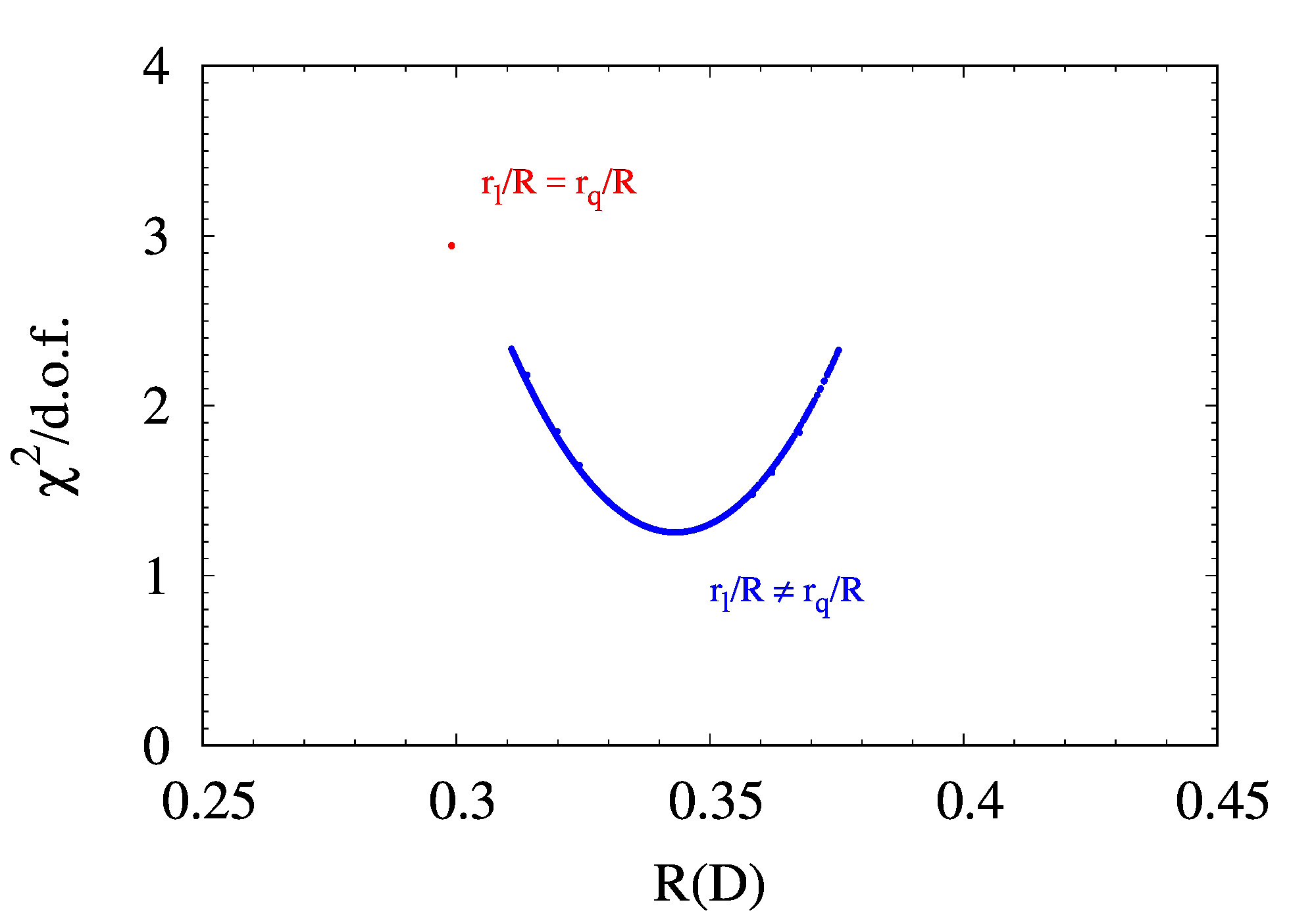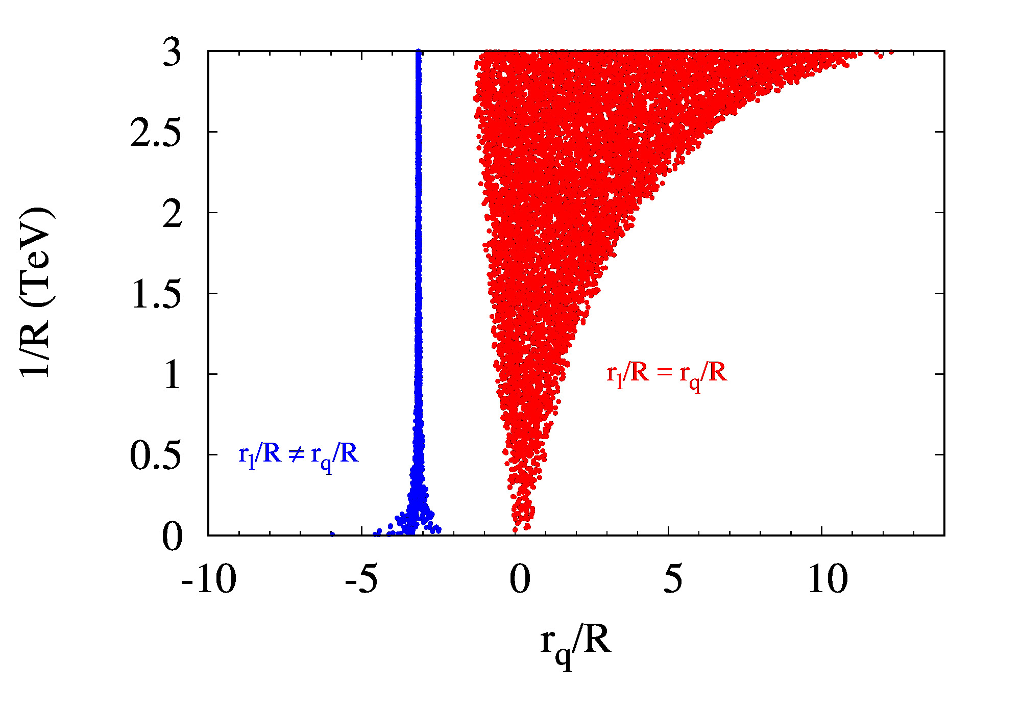
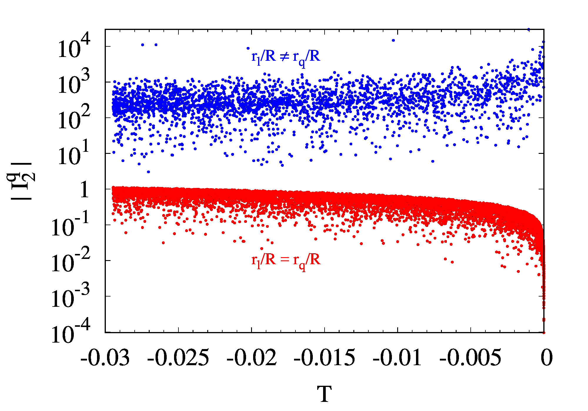
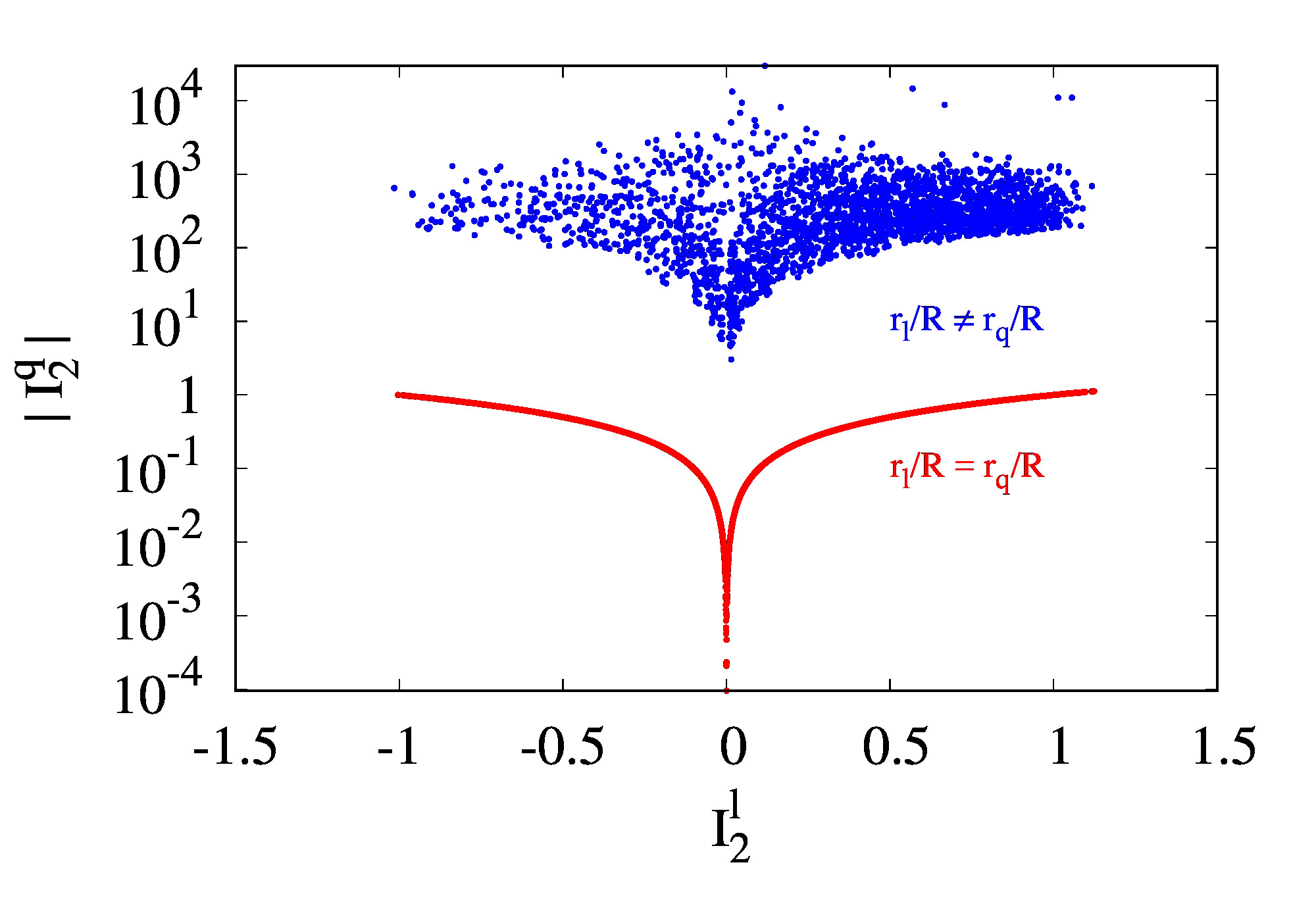
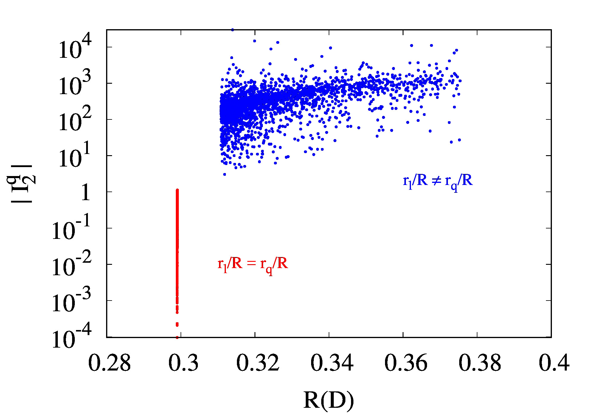
To see the effects of $r_{\ell}/R\neq r_{q}/R$ more dramatically, we compare the cases of $r_{\ell}/R=r_{q}/R$ and $r_{\ell}/R\neq r_{q}/R$ in Fig. 6. Figure 6 (a) shows that the allowed regions of $r_{q}/R$ are quite different from each other.

(a)	(b)
(c)	(d)

Figure 6: Comparisons of various parameter spaces for $r_{q}/R=r_{\ell}/R$ (red) and $r_{q}/R\neq r_{\ell}/R$ (blue) at $2\sigma$.

The effect of $r_{\ell}/R\neq r_{q}/R$ appears dramatically on $I_{2}^{q}$, as shown in Figs. 6 (b)-(d). As mentioned above, this is due to the constraints on the oblique parameters. If $r_{q}/R=r_{\ell}/R$, then $I_{2}^{q}=I_{2}^{\ell}$ and it should be kept small to satisfy the EWPT (Fig. 6 (b)). In case of $r_{q}/R\neq r_{\ell}/R$, $I_{2}^{q}$ can be very large compared to $I_{2}^{\ell}$ (Fig. 6 (c)). As a result, $R(D)$ is allowed to have large values to fit the data (Fig. 6 (d)).

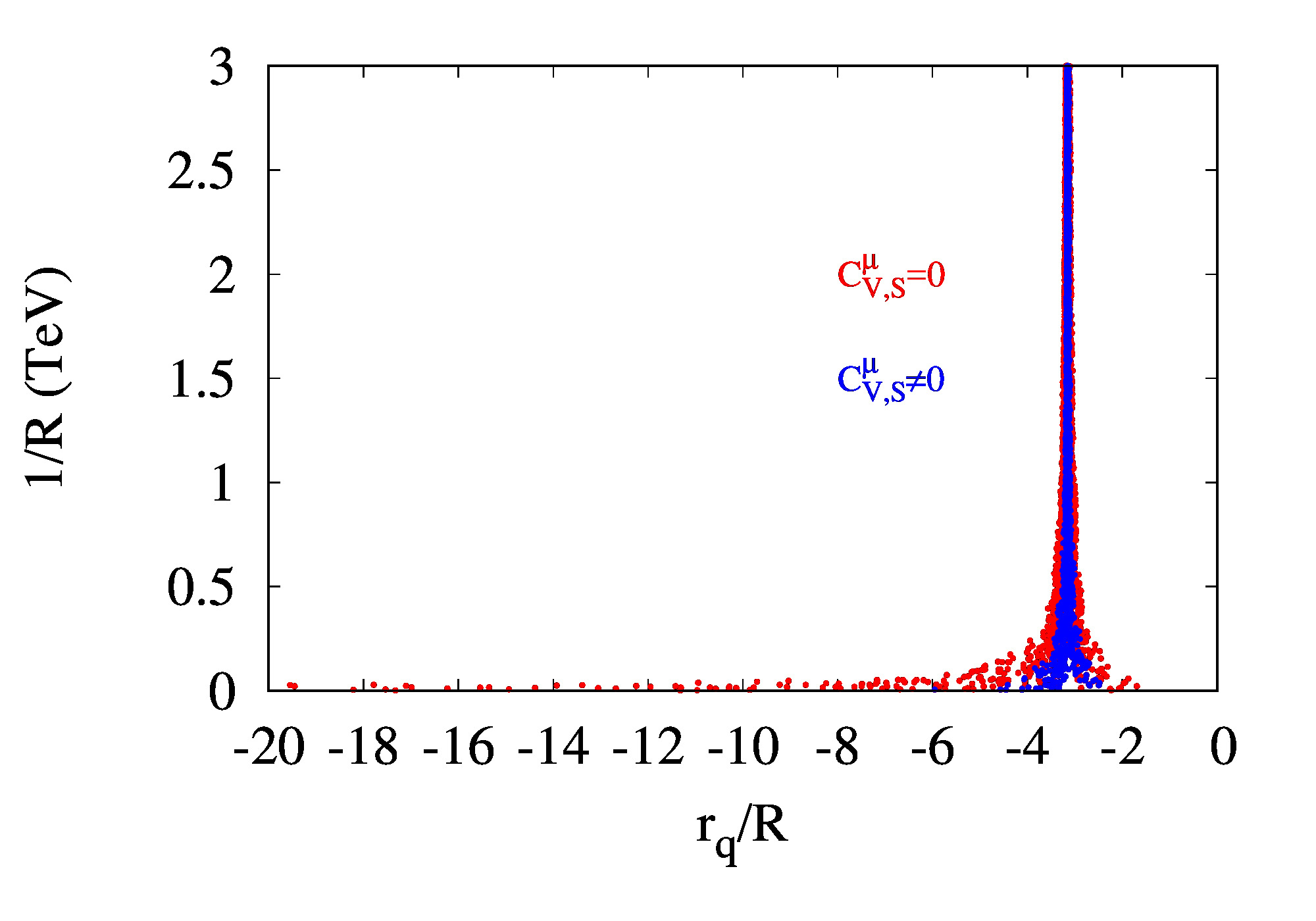
In our analysis $C_{V}^{\tau}=C_{V}^{\mu}$, and we checked the influence of nonzero $C_{V,S}^{\mu}$. Figure 7 shows some of the results.

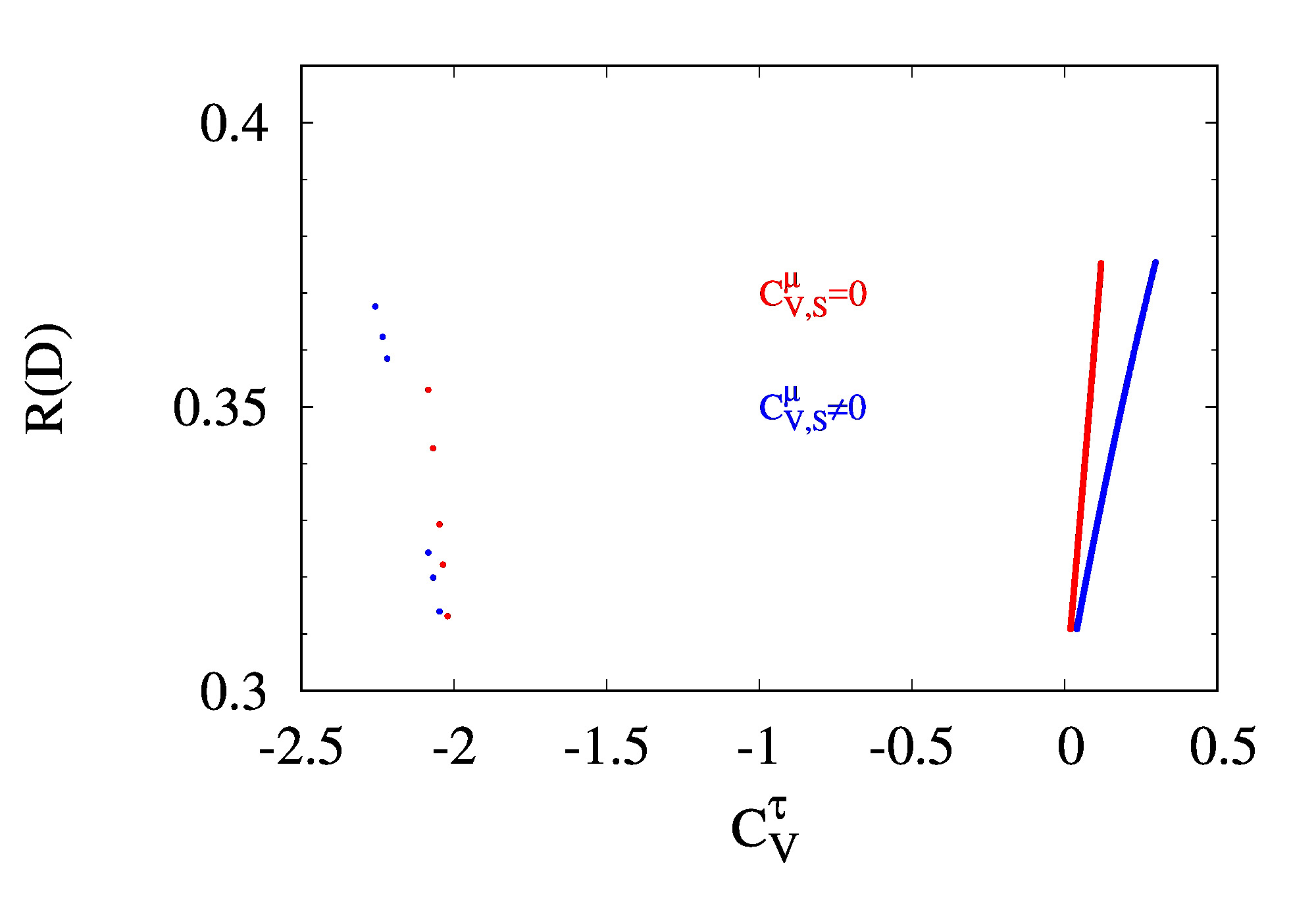(a)	(b)

Figure 7: Comparisons of parameter spaces for $C_{V,S}^{\mu}=0$ (red) and $C_{V,S}^{\mu}\neq 0$ (blue) at $2\sigma$.

Figure 7 (a) depicts $1/R$ vs $r_{q}/R$ while (b) does $R(D)$ vs $C_{V}^{\tau}$. We have similar figure for $R(D^{*})$ to Fig. 7 (b). Whether $C_{V,S}^{\mu}=0$ or not does not affect the observables including the polarizations so much, but the allowed range of $r_{q}/R$ or $C_{V}^{\tau}$ could be slightly different. The effect of $C_{S}^{\mu}$ is negligible because its values are very small compared to $C_{S}^{\tau}$. Note that $C_{S}^{\mu}$ is suppressed by $\sim m_{\mu}/m_{\tau}$ with respect to $C_{S}^{\tau}$. And the mixed terms of $(1+C_{V}^{\mu,\tau})C_{S}^{\mu,\tau}$ in Eq. (25) are the main source of a difference between $\tau\nu$ mode and $\mu\nu$ mode.

In this analysis we do not consider explicitly possible constraints from the flavor changing neutral currents (FCNC) involving $b$ quark sector, but it needs some comments. First, there is no FCNC at tree level because the BLT parameter $r_{q}$ is flavor independent. The effective couplings of the even KK mode of gauge bosons and the SM quarks can be written as the matrix in the flavor space Dasgupta

$$G^{(n)}={\rm diag}\Big{(}g_{r_{1}}^{X^{(n)}},g_{r_{2}}^{X^{(n)}},g_{r_{3}}^{X^{(n)}}\Big{)}~{},$$ (40)

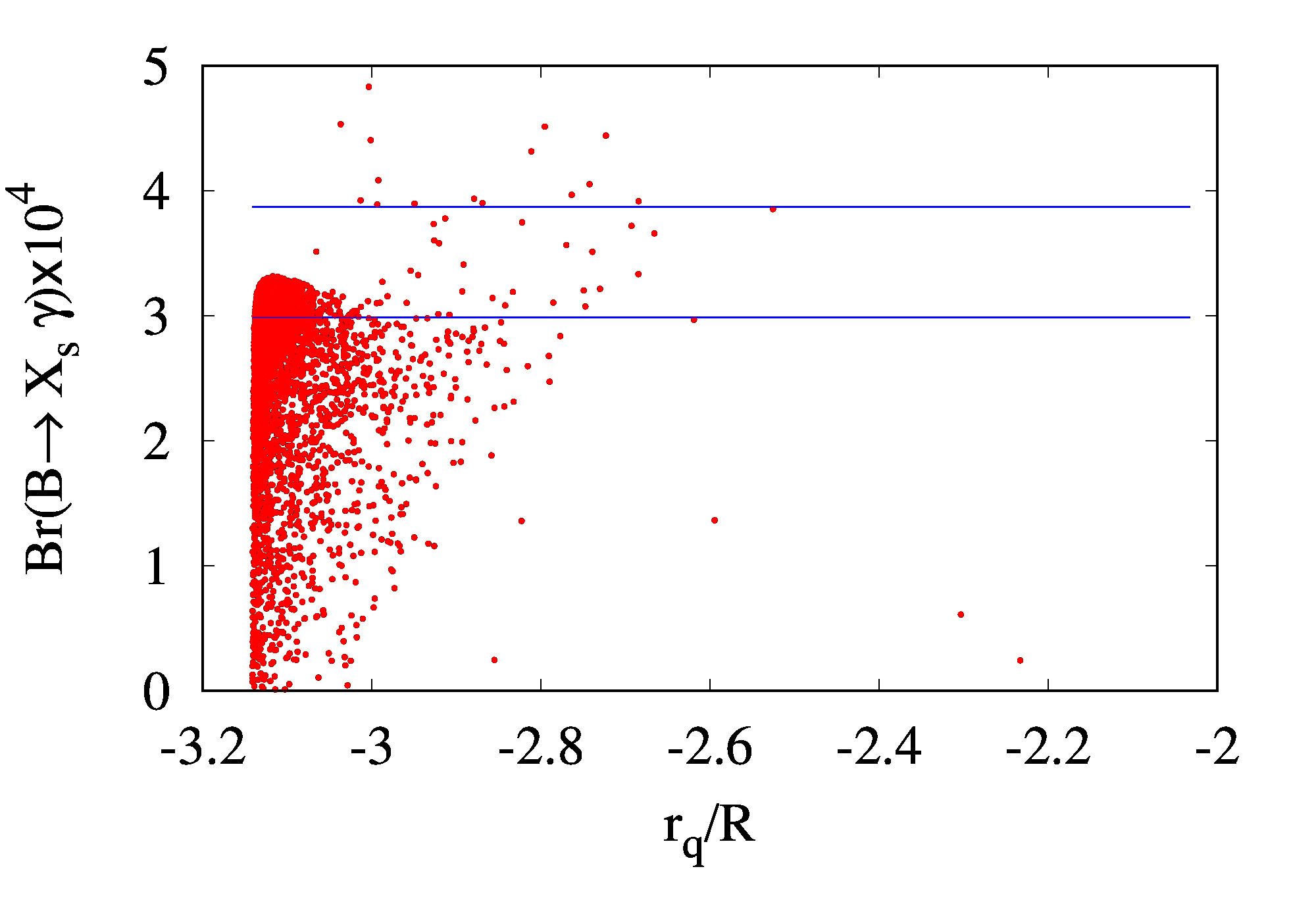
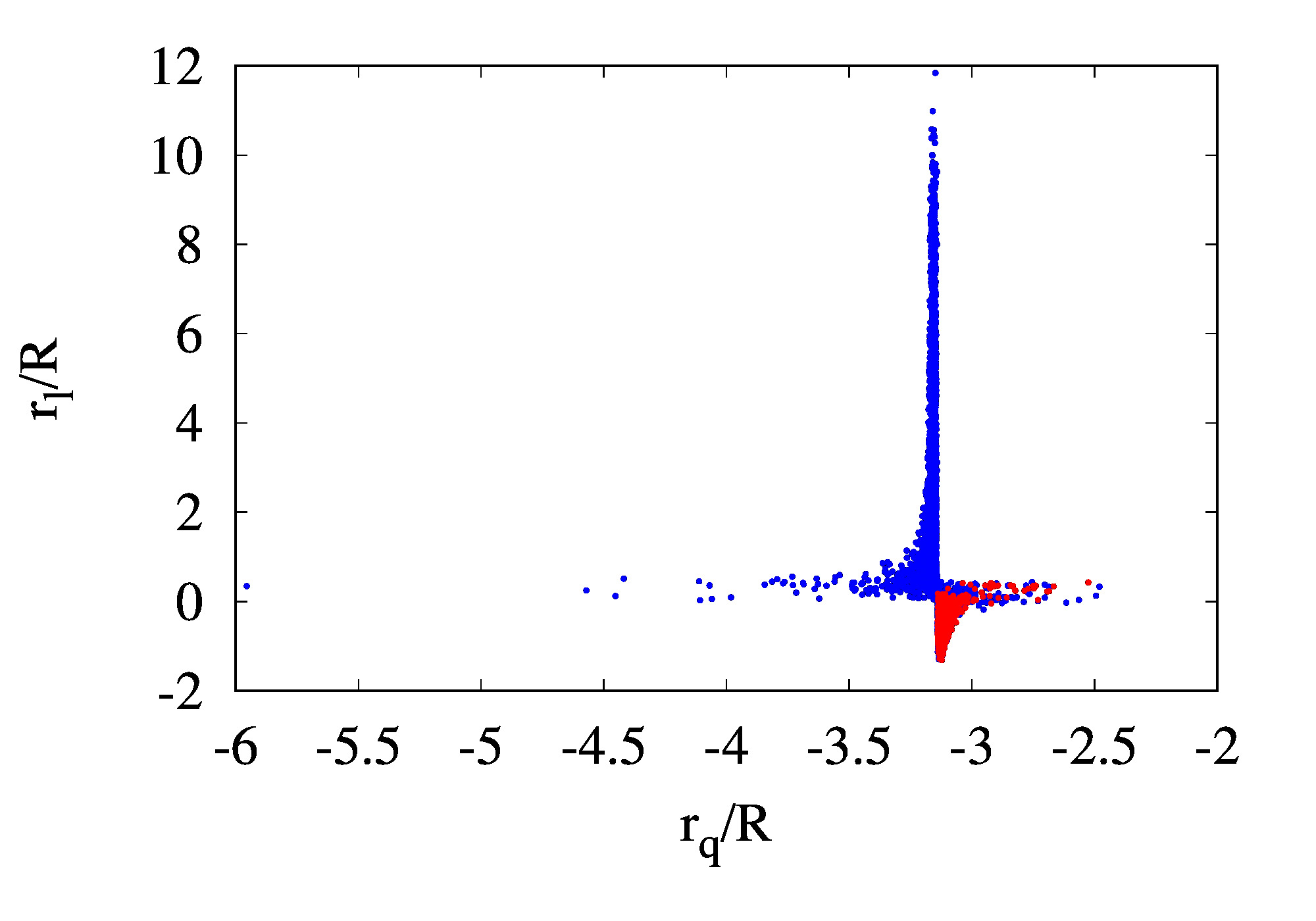
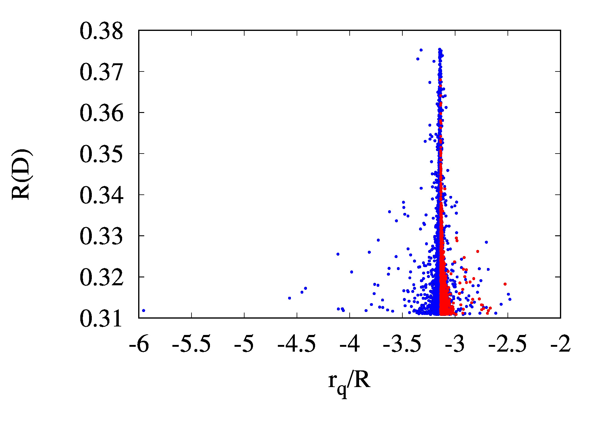
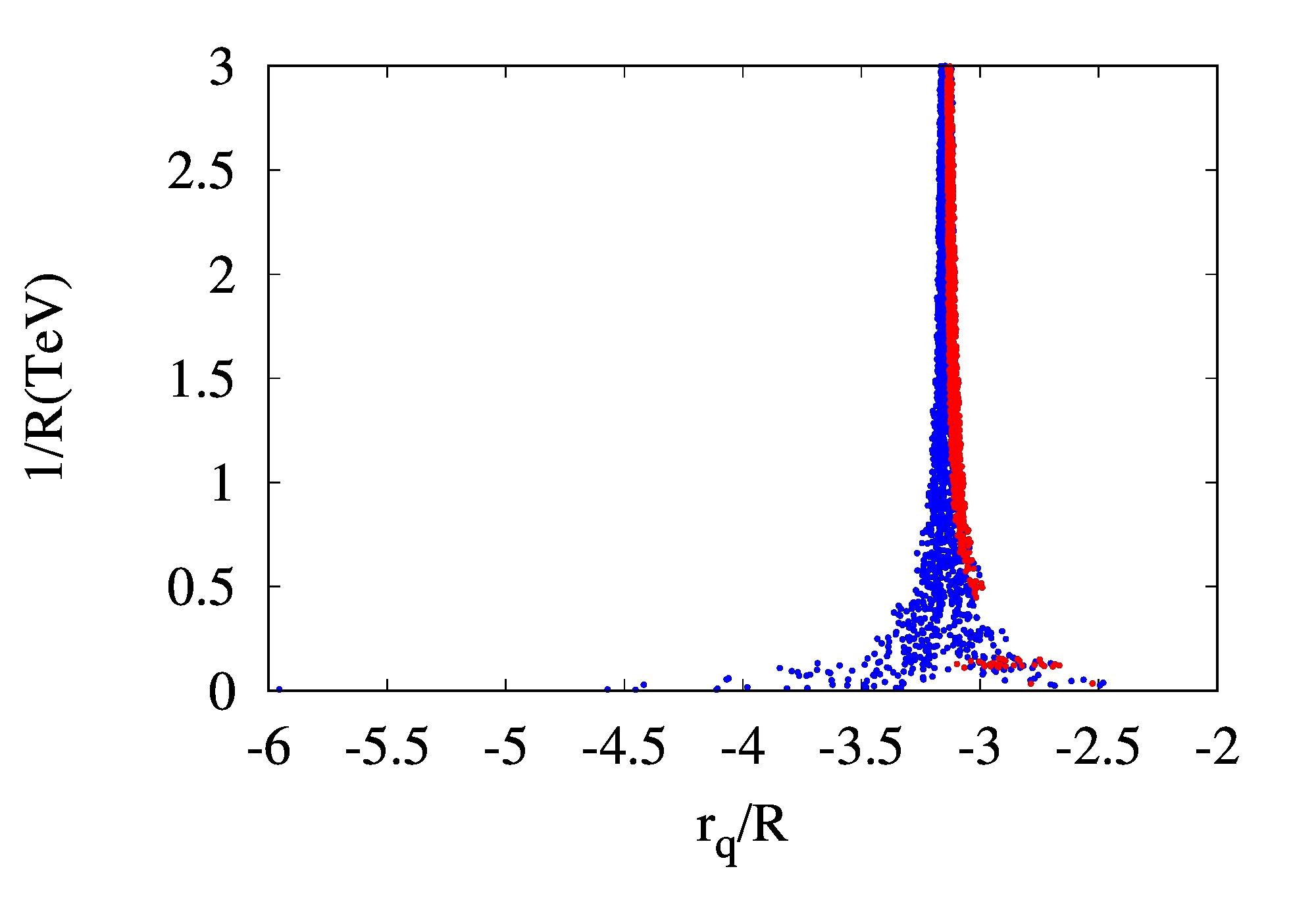
where $X^{(n)}=\gamma^{(n)},Z^{(n)}$ and $r_{1}=r_{2}=r_{3}=r_{q}$ in our case. The result is that $G^{(n)}$ is proportional to the identity matrix. Second, $B_{s}\to\mu^{+}\mu^{-}$ and $B\to X_{s}\gamma$ are investigated in Refs. Datta16 and Datta17 , respectively. The decay of $B_{s}\to\mu^{+}\mu^{-}$ or $B_{s}\to X_{s}\ell^{+}\ell^{-}$ involves both $I_{n}^{q}$ and $I_{n}^{\ell}$ while $B\to X_{s}\gamma$ does $I_{n}^{q}$ only. In the former case since $I_{n}^{q}$ and $I_{n}^{\ell}$ both contributes to the process one can expect that the constraint on $I_{n}^{\ell}$ would not be as strong as that from the oblique parameters. Actually in Ref. Datta16 the analysis was done with $r_{q}=r_{\ell}$. As one can see in Fig. 6 of Datta16 , the allowed parameter space for small $r_{V}$ is compatible with our results. One point that must be noticed is that the lower limit of $R^{-1}$ is about a few hundred GeV, which varies with $r_{V}$ and $r_{q,\ell}$ (see TABLE II of Datta16 ). In case of $r_{q}\neq r_{\ell}$, the allowed parameter space would be larger. In $B\to X_{s}\gamma$, only $I_{n}^{q}$ contributes to the process. According to the Ref. Datta17 , dominant contribution comes not from $I_{n}^{q}$ but from other overlap integrals, $I^{n}_{1,2}$ (see Eqs. (A10) and (A11) of Ref. Datta17 ). The integrals contain a factor of $\sqrt{1+r_{q}/(\pi R)}$ and we restrict the range of $r_{q}$ as $-\pi<r_{q}/R$ in considering ${\rm Br}(B\to X_{s}\gamma)$. In Fig. 8 we show the effects of ${\rm Br}(B\to X_{s}\gamma)$ on parameter space.

(a)	(b)
(c)	(d)

Figure 8: Constraints from experimental results of ${\rm Br}(B\to X_{s}\gamma)=(3.43\pm 0.21\pm 0.07)\times 10^{-4}$ Datta17 ; HFAG14 . Panel (a) shows the values of ${\rm Br}(B\to X_{s}\gamma)$ with the points of Fig. 1 but with $-\pi<r_{q}/R$. Blue horizontal lines are $2\sigma$ allowed bounds. In panels (b), (c) and (d) allowed regions by ${\rm Br}(B\to X_{s}\gamma)$ (red) are given, compared with those of Fig. 1 (blue).

We only consider the lowest KK mode contributions for convenience. As shown in Fig. 8 (b) positively large values of $r_{\ell}/R$ are not allowed. We find that a considerable amount of parameter space is forbidden, but still the value of $\chi^{2}_{\rm min}$ is almost the same and the best-fit values of the observables remain also unchanged. Third, $B_{s}$-${\bar{B}}_{s}$ mixing involves only $I_{n}^{q}$ and could provide a very strong constraint on $r_{q}$. The SM prediction of the mass difference $\Delta M_{s}$ MsSM ,

$$\Delta M_{s}^{\rm SM}=(20.01\pm 1.25)/{\rm ps}~{},$$ (41)

is by $1.8\sigma$ larger than the measured value Amhis ,

$$\Delta M_{s}^{\rm exp}=(17.757\pm 0.021)/{\rm ps}~{}.$$ (42)

Usually the NP gives positive contribution and $\Delta M_{s}$ puts much stronger bounds on NP than before because the updated SM prediction of $\Delta M_{s}$ gets larger Luzio . In our case $\Delta M_{s}$ is roughly $\sim(I_{n}^{q})^{4}(m_{W}/M_{KK})^{4}$ where $M_{KK}$ is the mass of the mediating KK particle. At the $2\sigma$ level, $\Delta M_{s}^{\rm exp}/(\Delta M_{s}^{\rm SM}-2\delta\Delta M_{s}^{\rm SM})-1\simeq 0.014$ where $\delta\Delta M_{s}^{\rm SM}$ is the $1\sigma$ deviation of $\Delta M_{s}^{\rm SM}$. One can naively guess that for $M_{KK}\sim 1~{}{\rm TeV}$ only order 1 of $I_{n}^{q}$ is allowed, which could severely constrain $r_{q}$. Further study on this issue is necessary to scrutinize the model.

V Conclusions

In conclusion, we investigated the $B\to D^{(*)}$ anomalies in the nmUED model. In the model, $n$th KK-modes of $W$-boson and scalar couple to a pair of zero-mode fermions to result in nonzero NP Wilson coefficients. We found that the nmUED model successfully fits the current data including $D^{*}$ polarizations, at the sacrifice of $r_{\ell}/R=r_{q}/R$. The EWPT plays a significant role in the model. Our main result is that the enhancement of the overlap integral in the quark sector is very crucial to explain the $B$ anomalies. If there would be a quite strong constraint on the quark sector (e.g. from the neutral meson mixing or whatever) then it could restrict the validity of the nmUED model seriously. We also found that the branching ratio ${\rm Br}(B_{c}\to\tau\nu)$ stays at a few percents, well below 10%. In our analysis $R(D)$ values have no overlap with the SM predictions at the $2\sigma$ level while $R(D^{*})$ touches the SM-allowed region. Future measurements of more observables would check further the validity of the nmUED model.

References

- (1) Y. Amhis et al. [HFLAV Collaboration], Eur. Phys. J. C 77, no. 12, 895 (2017).
- (2) J. P. Lees et al. [BaBar Collaboration], Phys. Rev. Lett. 109, 101802 (2012).
- (3) J. P. Lees et al. [BaBar Collaboration], Phys. Rev. D 88, no. 7, 072012 (2013).
- (4) M. Huschle et al. [Belle Collaboration], Phys. Rev. D 92, no. 7, 072014 (2015).
- (5) Y. Sato et al. [Belle Collaboration], Phys. Rev. D 94, no. 7, 072007 (2016).
- (6) S. Hirose [Belle Collaboration], Nucl. Part. Phys. Proc. 287-288, 185 (2017).
- (7) S. Hirose et al. [Belle Collaboration], Phys. Rev. Lett. 118, no. 21, 211801 (2017).
- (8) S. Hirose et al. [Belle Collaboration], Phys. Rev. D 97, no. 1, 012004 (2018).
- (9) A. Abdesselam et al. [Belle Collaboration], arXiv:1904.08794 [hep-ex].
- (10) R. Aaij et al. [LHCb Collaboration], Phys. Rev. Lett. 115, no. 11, 111803 (2015) Addendum: [Phys. Rev. Lett. 115, no. 15, 159901 (2015)].
- (11) R. Aaij et al. [LHCb Collaboration], Phys. Rev. D 97, no. 7, 072013 (2018).
- (12) Average of and for Spring 2019, Heavy Flavor Averaging Group, https://hflav-eos.web.cern.ch/hflav-eos/semi/spring19/html/RDsDsstar/RDRDs.html
- (13) J. P. Lee, Phys. Rev. D 96, no. 5, 055005 (2017).
- (14) A. Crivellin, C. Greub and A. Kokulu, Phys. Rev. D 86, 054014 (2012); Phys. Rev. D 87, no. 9, 094031 (2013); A. Crivellin, J. Heeck and P. Stoffer, Phys. Rev. Lett. 116, no. 8, 081801 (2016).
- (15) P. Biancofiore, P. Colangelo and F. De Fazio, Phys. Rev. D 87, no. 7, 074010 (2013).
- (16) J. M. Cline, Phys. Rev. D 93, no. 7, 075017 (2016).
- (17) M. A. Ivanov, J. G. Körner and C. T. Tran, Phys. Rev. D 94, no. 9, 094028 (2016); Phys. Rev. D 95, no. 3, 036021 (2017).
- (18) C. H. Chen and T. Nomura, Eur. Phys. J. C 77, no. 9, 631 (2017).
- (19) S. Iguro and K. Tobe, Nucl. Phys. B 925, 560 (2017).
- (20) I. Dorner, S. Fajfer, N. Konik and I. Niandi, JHEP 1311, 084 (2013).
- (21) R. Alonso, B. Grinstein and J. Martin Camalich, JHEP 1510, 184 (2015).
- (22) M. Bauer and M. Neubert, Phys. Rev. Lett. 116, no. 14, 141802 (2016).
- (23) R. Barbieri, G. Isidori, A. Pattori and F. Senia, Eur. Phys. J. C 76, no. 2, 67 (2016).
- (24) L. Di Luzio, A. Greljo and M. Nardecchia, Phys. Rev. D 96, no. 11, 115011 (2017).
- (25) L. Calibbi, A. Crivellin and T. Li, Phys. Rev. D 98, no. 11, 115002 (2018).
- (26) D. Beirevi, I. Dorner, S. Fajfer, N. Konik, D. A. Faroughy and O. Sumensari, Phys. Rev. D 98, no. 5, 055003 (2018).
- (27) R. Barbieri, C. W. Murphy and F. Senia, Eur. Phys. J. C 77, no. 1, 8 (2017).
- (28) D. Buttazzo, A. Greljo, G. Isidori and D. Marzocca, JHEP 1711, 044 (2017).
- (29) M. Bordone, C. Cornella, J. Fuentes-Martin and G. Isidori, Phys. Lett. B 779, 317 (2018).
- (30) S. Matsuzaki, K. Nishiwaki and K. Yamamoto, [arXiv:1903.10823 [hep-ph]].
- (31) E. Megias, M. Quiros and L. Salas, JHEP 1707, 102 (2017).
- (32) E. Megias, M. Quiros and L. Salas, Phys. Rev. D 96, no. 7, 075030 (2017).
- (33) G. D’Ambrosio and A. M. Iyer, Eur. Phys. J. C 78, no. 6, 448 (2018).
- (34) M. Blanke and A. Crivellin, Phys. Rev. Lett. 121, no. 1, 011801 (2018).
- (35) X. W. Kang, T. Luo, Y. Zhang, L. Y. Dai and C. Wang, Eur. Phys. J. C 78, no. 11, 909 (2018).
- (36) Z. R. Huang, Y. Li, C. D. Lu, M. A. Paracha and C. Wang, Phys. Rev. D 98, no. 9, 095018 (2018).
- (37) D. Bardhan and D. Ghosh, Phys. Rev. D 100, no. 1, 011701 (2019) doi:10.1103/PhysRevD.100.011701 [arXiv:1904.10432 [hep-ph]].
- (38) M. Tanaka and R. Watanabe, Phys. Rev. D 82, 034027 (2010).
- (39) M. Tanaka and R. Watanabe, Phys. Rev. D 87, no. 3, 034028 (2013).
- (40) A. Abdesselam et al. [Belle Collaboration], arXiv:1903.03102 [hep-ex].
- (41) A. K. Alok, D. Kumar, S. Kumbhakar and S. U. Sankar, Phys. Rev. D 95, no. 11, 115038 (2017).
- (42) H. C. Cheng, K. T. Matchev and M. Schmaltz, Phys. Rev. D 66, 036005 (2002).
- (43) F. del Aguila, M. Perez-Victoria and J. Santiago, Acta Phys. Polon. B 34, 5511 (2003).
- (44) F. del Aguila, M. Perez-Victoria and J. Santiago, JHEP 0302, 051 (2003).
- (45) T. Flacke, A. Menon and D. J. Phalen, Phys. Rev. D 79, 056009 (2009).
- (46) A. Datta, U. K. Dey, A. Shaw and A. Raychaudhuri, Phys. Rev. D 87, no. 7, 076002 (2013).
- (47) A. Datta and A. Shaw, Mod. Phys. Lett. A 31, no. 32, 1650181 (2016).
- (48) A. Datta and A. Shaw, Phys. Rev. D 93, no. 5, 055048 (2016).
- (49) A. Datta et al. [Indian Association for the Cultivation of Science Collaboration], Phys. Rev. D 95, no. 1, 015033 (2017).
- (50) A. Biswas, A. Shaw and S. K. Patra, Phys. Rev. D 97, no. 3, 035019 (2018).
- (51) S. Dasgupta, U. K. Dey, T. Jha and T. S. Ray, Phys. Rev. D 98, no. 5, 055006 (2018).
- (52) T. Jha and A. Datta, JHEP 1503, 012 (2015).
- (53) M. Blanke, A. Crivellin, S. de Boer, T. Kitahara, M. Moscati, U. Nierste and I. Niandi, Phys. Rev. D 99, no. 7, 075006 (2019); arXiv:1905.08253 [hep-ph].
- (54) S. Aoki et al., Eur. Phys. J. C 77, no. 2, 112 (2017).
- (55) F. U. Bernlochner, Z. Ligeti, M. Papucci and D. J. Robinson, Phys. Rev. D 95, no. 11, 115008 (2017) Erratum: [Phys. Rev. D 97, no. 5, 059902 (2018)].
- (56) R. Alonso, B. Grinstein and J. Martin Camalich, Phys. Rev. Lett. 118, no. 8, 081802 (2017).
- (57) A. G. Akeroyd and C. H. Chen, Phys. Rev. D 96, no. 7, 075011 (2017).
- (58) T. Flacke and C. Pasold, Phys. Rev. D 85, 126007 (2012).
- (59) T. Flacke, K. Kong and S. C. Park, JHEP 1305, 111 (2013).
- (60) A. Datta, K. Nishiwaki and S. Niyogi, JHEP 1401, 104 (2014).
- (61) U. K. Dey and T. Jha, Phys. Rev. D 94, no. 5, 056011 (2016).
- (62) M. Baak et al. [Gfitter Group], Eur. Phys. J. C 74, 3046 (2014).
- (63) T. Flacke, D. W. Kang, K. Kong, G. Mohlabeng and S. C. Park, JHEP 1704, 041 (2017).
- (64) Y. Amhis et al. [Heavy Flavor Averaging Group (HFAG)], arXiv:1412.7515 [hep-ex].
- (65) L. Di Luzio, M. Kirk and A. Lenz, Phys. Rev. D 97, no. 9, 095035 (2018).
- (66) L. Di Luzio, M. Kirk and A. Lenz, arXiv:1811.12884 [hep-ph].