Computational Many-Body Physics via $\mathcal{M}_{2^{q}}$ Algebra

Abstract

The many-body Hamiltonians and other fermionic physical observables are expressed in terms of fermionic creation and annihilation operators, which, at an abstract level, form the algebra of Canonical Anti-commutation Relations. If the one-particle Hilbert space is $q$-dimensional, then this algebra is canonically isomorphic with the ordinary algebra $\mathcal{M}_{2^{q}}$ of $2^{q}\times 2^{q}$ matrices with complex entries. In this work, we present a method that makes this isomorphism explicit. This supplies concrete matrix representations of various many-body operators without involving the traditional Fock space representation. The result is a steep simplification of the many-body exact diagonalization codes, which is a significant step towards the soft-coding of generic fermionic Hamiltonians. Pseudo-code implementing matrix representations of various many-body operators are supplied and Hubbard-type Hamiltonians are worked out explicitly.

I Introduction

Local physical observables of fermionic systems are expressed as products and sums of creation $a_{n}^{\ast}$ and annihilation $a_{n}$ operators. The latter satisfy the canonical anti-commutation relations which automatically enforce Pauli’s exclusion principle. The set of local fermionic physical observabales can be closed to and given the structure of a $C^{\ast}$-algebra, called the canonical anti-commutation relations algebra, or in short CAR-algebra BratelliBook2 . In the Heisenberg approach, one formulates the dynamics of fermions directly on the CAR-algebra and a many-body physical system is completely specified by a tuple $(\alpha,\mathcal{T})$, where $\alpha$ is a group homomorphism $\alpha\,:\,\mathbb{R}\rightarrow{\rm Aut}({\rm CAR})$, specifying the time evolution of the physical observables, and $\mathcal{T}$ is a state invariant w.r.t. the $\alpha$-dynamics. In the Schroedinger picture, the dynamics of fermions is formulated on the anti-symmetric sector of the Fock space, which supplies a natural representation space for the CAR-algebra. Note that in Heisenberg’s picture there is no place for Hilbert spaces and representations, and this observation is the starting point for our work. While we focus here at computational many-body aspects, this subtle but essential difference between the two pictures of quantum phenomena has conceptual consequences, as highlighted recently by Haldane in HaldaneJMP2018 .

At the computational level, the difference manifests as follows: In the Heisenberg picture, one seeks a direct homomorphism that embeds the algebra of observables in a matrix algebra. In Schroedinger’s picture, the matrix representations are generated by acting with the operators on the basis of the Hilbert space. To see the major difference, let us consider a generic system where the fermions populate a discrete set $X$ of some physical space. We denote by $q$ the cardinal of $X$. The generic many-body observables take the form:

$$A=\sum_{J,J^{\prime}\subseteq X}a_{J,J^{\prime}}\prod_{x\in J}a_{x}^{\ast}\prod_{x^{\prime}\in J^{\prime}}a_{x^{\prime}}.$$ (1)

Then in the Schroedinger picture, one will generate the $2^{q}\times 2^{q}$ matrix representation by looping over the occupation basis:

$$\langle n^{\prime}_{1}n^{\prime}_{2}\ldots n^{\prime}_{q}|A|n_{1}n_{2}\ldots n_{q}\rangle,\quad n^{\prime}_{i},n_{i}\in\{0,1\},$$ (2)

using, for example, the action of the generators on the basis:

$$a^{\ast}_{m}|n_{1}\ldots n_{m}\ldots n_{q}\rangle$$ (3)

$$\qquad=(-1)^{\alpha}(n_{m}\oplus 1){\rm mod}\,2\,|n_{1}\ldots n_{m}+1\ldots n_{q}\rangle,$$

where $\oplus$ is addition mod 2. In a successful Heisenberg program, however, one will use the embedding homomorphism to explicitly specify the entire $2^{q}\times 2^{q}$ matrix in one step. When the many-body operator has a simple structure, the action of $\prod_{x\in J}a_{x}^{\ast}\prod_{x^{\prime}\in J^{\prime}}a_{x^{\prime}}$ on the occupation basis can be computed by hand and then the result can be integrated in the computer codes. However, this is typically hard-coded and the entire task needs to be repeated when presented with a different operator. A soft-code, by definition, is one that can diagonalize any many-body observable $A$ based on an input file that contains the subsets $J$ and $J^{\prime}$ of $X$, as well as the associated coefficients $a_{J,J^{\prime}}$. In the Schroedinger approach, the only way to achieve such soft-coding is to repeatedly apply the generators on the occupation basis but this leads to highly inefficient algorithms. This highlights one of the advantages of the Heisenberg approach, which become extremely useful when dealing with complicated Hamiltonians such as the ones often occuring in the research on topological phases of matters. For example, the Fidkowski-Kitaev Hamiltonians FidkowskiPRB2010 ; FidkowskiPRB2011 contains products of as many as 8 generators! The model Hamiltonians for higher fractional Hall sequences ProdanPRB2009 present the same if not even higher level of complexity.

In this work, we exploit a well-know isomorphism between CAR and $M_{2^{\infty}}$ algebras DavidsonBook to derive matrix representations of generic products of creation and annihilation operators. Explicit analytic formulas are supplied for several key products of generators, which will enable one to analytically translate any many-fermion Hamiltonian into a matrix form. For the reader’s convenience, we exemplify the algorithms with concrete pieces of code and we work out several interesting many-fermion eigen-problems.

In our opinion, the benefits of the proposed approach can materialize in two extreme settings. The first one, is that of small-scale computations involving complex Hamiltonians. For example, the search and characterization of topological boundary modes in correlated systems require precisely this type of computations, especially when the goal is to validate their robustness against arbitrary interaction potentials. The challenge for this type of research is that the one-particle Hilbert spaces and the many-body Hamiltonians can vary drastically from one application to another and it is precisely this challenge that is addressed by our approach. The second setting is that of large-scale computations with standard two-body potentials, such as the Coulomb potential. Since our approach supplies formal matrix representations of the Hamiltonians, one can estimate the sparseness of the matrices (see for example Fig. 1) and then decide more easily on the optimal linear-algebra package to be used. One can also estimate more accurately the numerical errors and speed-up of the computations can result from the analytically determined action of the whole Hamiltonian on vectors.

II Background

II.1 The Algebra of Canonical Anti-Commutation Relations

The algebra of canonical anti-commutation relations (CAR) is defined BratelliBook2 by a linear map $a:\mathcal{H}\rightarrow\mathcal{B}(\mathcal{H}^{\prime})$ from a Hilbert space $\mathcal{H}$ onto the algebra of linear maps over another Hilbert space $\mathcal{H}^{\prime}$, satisfying the following algebraic relations:

$$\begin{array}[]{c}a(f)a(g)+a(g)a(f)=0\\ a(f)^{*}a(g)+a(g)a(f)^{*}=(g,f)1.\end{array}$$ (4)

for all $f,\ g\in\mathcal{H}$. Here and throughout, $(\ ,\ )$ denotes the scalar product on $\mathcal{H}$. The CAR-algebra is the $C^{*}$-algebra generated by $\{a(f):f\in\mathcal{H}\}$ modulo relations (4), endowed with the $\ast$-operation and the $C^{*}$-norm borrowed from $\mathcal{B}(\mathcal{H}^{\prime})$. Up to an isomorphism, this definition is completely independent of the concrete representations of the Hilbert spaces. In many-body physics, $\mathcal{H}$ represents the one-particle Hilbert space and $\mathcal{H}^{\prime}$ is chosen as the Fock-space and one says that $a(f)^{\ast}$ creates a fermion in the quantum state $f$, while $a(f)$ destroys a fermion in quantum state $f$.

For condensed matter physicists, perhaps a more familiar representation of the CAR-algebra can be given in the following terms. Let $\{f_{i}\}_{i=\overline{0,\infty}}$ denote an orthonormal basis on $\mathcal{H}$ and let $a_{i}=a(f_{i})$. Then the $a_{i}$’s satisfy the familiar anti-commutation relations:

$$a_{i}a_{j}+a_{j}a_{i}=a_{i}^{\ast}a_{j}^{\ast}+a_{j}^{\ast}a_{i}^{\ast}=0,\ a_{i}^{\ast}a_{j}+a_{j}a_{i}^{\ast}=\delta_{ij}\,1.$$ (5)

If one prefers to maintain the liberty of choosing and changing the basis of the Hilbert space, the first representation in Eq. 4 is definitely more preferable.

We will denote the CAR-algebra over a finite dimensional Hilbert space $\dim\mathcal{H}_{q}=q<\infty$ by $CAR(q)$. Throughout our presentation, we will be consistent and enumerate the elements of the orthonormal basis starting from 0 and ending at $q-1$. In other words, we will label the orthonormal basis of $\mathcal{H}_{q}$ as $f_{0}$, $f_{1}$, …, $f_{q-1}$.

The CAR-algebra is a $C^{\ast}$-algebra, that is, it is closed under the addition, multiplication and the $\ast$-transformation (or dagger-operation). The CAR-algebra also comes equipped with a norm but, since we are mainly considering finite CAR-algebras, this norm will not play any special role here. If $a(f),a(g),\ldots$ are some elements of $CAR(q)$, we will denote by $C^{\ast}\big{(}a(f),a(g),\ldots\big{)}$ the sub-algebra generated by them. Henceforth, $C^{\ast}\big{(}a(f),a(g),\ldots\big{)}$ contains all elements in $CAR(q)$ that can be formed through sums, multiplications and $\ast$-transformations of $a(f)$, $a(g)$, …. In particular, let us point out that $CAR(q)$ can be naturally embedded in $CAR(q+1)$ and this sets an inductive tower which enable one to define $CAR(\mathcal{H}_{\infty})$ as its inductive limit.

II.2 The algebra $\mathcal{M}_{2^{\infty}}$

Let $\mathcal{M}_{2}$ denote the algebra of $2\times 2$ matrices with complex entries. Then $\mathcal{M}_{2^{q}}=\mathcal{M}_{2}\otimes\mathcal{M}_{2}\ldots\otimes\mathcal{M}_{2}=\mathcal{M}_{2}^{\otimes q}$, which is isomorphic to the algebra of $2^{q}\times 2^{q}$ matrices with complex entries. Note that $\mathcal{M}_{2^{q}}$ can be embedded in $\mathcal{M}_{2^{q+1}}$ as $\left({}^{\mathcal{M}_{2^{q}}}_{0}\ {}^{0}_{\mathcal{M}_{2^{q}}}\right)$ and, as such, one can set an inductive tower and define the UHF-algebra $\mathcal{M}_{2^{\infty}}$ as its inductive limit. The result is one of the most studied $C^{\ast}$-algebras in the mathematics literature. For example, its K-theory was worked out in RenaultBook (see also DavidsonBook ).

We now introduce notations and conventions for our exposition. For $A\in\mathcal{M}_{2}$ we choose to write $A=\left({}^{A_{00}}_{A_{10}}\ {}^{A_{01}}_{A_{11}}\right)$. As a linear space, $\mathcal{M}_{2^{q}}$ is generated by the system of units

$$\big{\{}E^{(q)}_{mn}\big{\}}_{m,n=0,\ldots,2^{q}-1},$$ (6)

where $E^{(q)}_{mn}$ is the $2^{q}\times 2^{q}$ matrix with entry 1 at position $(m,n)$ and 0 in rest. The system of units satisfies the usual algebraic relations:

$$E^{(q)}_{mn}\,E^{(q)}_{m^{\prime}n^{\prime}}=\delta_{nm^{\prime}}\,E^{(q)}_{mn^{\prime}}.$$ (7)

The system of units for $\mathcal{M}_{2}$ will be denoted by $\{e_{\alpha\beta}\}_{\alpha,\beta=0,1}.$

II.3 The link between the algebras

Theorem 1

$CAR(q)$ is isomorphic to $\mathcal{M}_{2^{q}}$ for all $q\in\mathbb{N}$.

Proof. A detailed proof can be found in Kenneth Davidson’s monograph DavidsonBook . It will be, however, very instructive and helpful to present the proof in details once again here. Henceforth, let $f_{0},f_{1},\ldots,f_{q-1}$ be an orthonormal basis of $\mathcal{H}_{q}$ and set $a_{i}=a(f_{i})$. Then $CAR(q)$ is simply $C^{\ast}\big{(}a_{0},a_{1},\ldots,a_{q-1}\big{)}$. Our first task is to define a new set of generator that commute with each other rather than anti-commute. This can be accomplished via a Jordan-Wigner type transformation, whose main mechanism is recalled below.

Let $f$ be a normalized vector from $\mathcal{H}$ and let:

$$n_{f}\coloneqq a(f)^{\ast}a(f).$$ (8)

Since $a(f)^{2}=0$ and $a(f)^{\ast}a(f)+a(f)a(f)^{\ast}=1$, by multiplying the latter by $a(f)a(f)^{\ast}$, one obtains $n_{f}^{2}=n_{f}$. In other words, $n_{f}$ is an idempotent for any norm-one vector $f$ from $\mathcal{H}_{q}$. In fact, $n_{f}$ is an orthogonal projector because $n_{f}^{\ast}=n_{f}$. Furthermore,

$$a(f)a(f)^{\ast}=1-a(f)^{\ast}a(f)=1-e(f),$$ (9)

hence $a(f)a(f)^{\ast}$ is the orthogonal complement of $n_{f}$:

$$n_{f}^{\bot}\coloneqq a(f)a(f)^{\ast},\ n_{f}n_{f}^{\bot}=0,\ n_{f}+n_{f}^{\bot}=1.$$ (10)

Consider now another vector $g$ from $\mathcal{H}_{q}$ which is orthogonal on $f$, $(f,g)=0$. One can verify directly that $a(g)$ commutes with $n_{f}$ (hence also with $n_{f}^{\bot}$) but of course, $a(g)$ does not commute with $a(f)$. This can be fixed as follows. Define:

$$v\coloneqq n_{f}^{\bot}-n_{f},$$ (11)

with the following obvious properties:

$$v^{*}=v,\ v^{2}=1,\ va(f)=-a(f)v,\ va(f)^{*}=-a(f)^{*}v.$$ (12)

If $va(g)$ is considered instead of $a(g)$, then:

$$va(g)a(f)=-va(f)a(g)=a(f)va(g).$$ (13)

Similarly:

$$va(g)a(f)^{*}=-va(f)^{*}a(g)=a(f)^{*}va(g).$$ (14)

Hence, the substitution $a(g)\rightarrow va(g)$ made the operators commute. This is the essence of the Jordan-Wigner transformation.

Returning now to $C^{*}\big{(}a_{0},a_{1},\ldots,a_{q-1}\big{)}$, we can define a set of commuting generators by iterating the above construction. This leads us to the following substitutions:

$$a_{i}\rightarrow v_{i}a_{i},$$ (15)

where $v_{0}=1$ and:

$$v_{i}=(n_{i-1}^{\bot}-n_{i-1})v_{i-1},\ v_{i}^{\ast}=v_{i},\ v_{i}^{2}=1,\ i=1,\ldots,q-1,$$ (16)

with $n_{i}=a_{i}^{\ast}a_{i}$. It is important to keep in mind that $n_{i}$’s are all commuting orthogonal projections. The conclusion so far is that:

$$C^{\ast}\big{(}a_{0},a_{1},\ldots,a_{q-1}\big{)}=C^{\ast}\big{(}v_{0}a_{0},v_{1}a_{1},\ldots,v_{q-1}a_{q-1}\big{)},$$ (17)

and now all the generators commute with each other. This concludes the step of the proof that involves the Jordan-Wigner transformation.

The next step is to look at the sub-algebra generated by each of these generators. Because of the anti-commution relations, one readily finds that $C^{*}\big{(}v_{i}a_{i}\big{)}$ coincides with the $\mathbb{C}$-linear span of just four operators:

$$C^{*}\big{(}v_{i}a_{i}\big{)}=\mathbb{C}\mathrm{-Span}\big{\{}n_{i},n_{i}^{\bot},v_{i}a_{i},v_{i}a_{i}^{\ast}\big{\}}.$$ (18)

Furthermore, if one sets:

$$e^{(i)}_{11}=n_{i},\ e^{(i)}_{00}=n_{i}^{\bot},\ e^{(i)}_{01}=v_{i}a_{i},\ e^{(i)}_{10}=v_{i}a_{i}^{*},$$ (19)

then

$$e^{(i)}_{\alpha\beta}e^{(i)}_{\alpha^{\prime}\beta^{\prime}}=\delta_{\beta\alpha^{\prime}}e^{(i)}_{\alpha\beta^{\prime}}$$ (20)

which are exactly the algebraic relations satisfied by the generators of $\mathcal{M}_{2}$. Hence, Eq. 20 defines an explicit isomorphic mapping of $\mathcal{M}_{2}$ into $C^{*}\big{(}v_{i}a_{i}\big{)}$.

The last step of the proof involves the following elements of $CAR(q)$:

$$E^{(q)}_{\varphi,\psi}=e^{(0)}_{\varphi(0)\psi(0)}e^{(1)}_{\varphi(1)\psi(1)}\ldots e^{(q-1)}_{\varphi(q-1)\psi(q-1)},$$ (21)

where $\varphi$ and $\psi$ are two functions of the type:

$$\varphi,\ \psi:\big{\{}0,1,\ldots,q-1\big{\}}\rightarrow\{0,1\}.$$ (22)

Note that there are exactly $2^{q}$ distinct such functions and one can verify explicitly that (21) span the entire $CAR(q)$ as well as that:

$$E^{(q)}_{\varphi,\psi}\ E^{(q)}_{\varphi^{\prime}\psi^{\prime}}=\delta_{\psi\varphi^{\prime}}\ E^{(q)}_{\varphi\psi^{\prime}},$$ (23)

which are precisely the algebraic relations (7) defining the generators of $\mathcal{M}_{2^{q}}$. The conclusion is that:

$$\left\{E^{(q)}_{\varphi,\psi}:\varphi,\ \psi:\big{\{}0,\ldots,q-1\big{\}}\rightarrow\big{\{}0,1\big{\}}\right\}$$ (24)

supply an explicit isomorphic mapping of $\mathcal{M}_{2^{q}}$ into $CAR(q)$. Furthermore, this mapping respects the embedding of $CAR(q)$ into $CAR(q+1)$ and of $\mathcal{M}_{2^{q}}$ into $\mathcal{M}_{2^{q+1}}$, hence the inductive towers are isomorphic and their limits are isomorphic as $C^{\ast}$-algebras Effros1979 . $\square$

III Practical Representations

For practical applications, we need to devise an efficient way to account for all $\varphi$’s and $\psi$’s appearing in Eq. 24.

Proposition 1

Let $n$ be an integer between $0$ and $2^{q}-1$. Let:

$$n=\alpha_{0}\cdot 2^{0}+\alpha_{1}\cdot 2^{1}+\ldots\alpha_{q-1}\cdot 2^{q-1},\quad\alpha_{i}\in\big{\{}0,1\big{\}},$$ (25)

be its unique binary representations and define:

$$\mathfrak{b}_{n}:\big{\{}0,\ldots,q-1\big{\}}\rightarrow\big{\{}0,1\big{\}},\ \mathfrak{b}_{n}(i)=\alpha_{i},$$ (26)

to be the function which outputs the binary digits of $n$. Then, when $n$ is varied from $0$ to $2^{q}-1$, the $\mathfrak{b}_{n}$’s generate all the possible functions $\varphi$’s and $\psi$’s appearing in Eq. 24.

Remark 1

We introduce the following important conventions. Firstly, we will identify the elements $e^{(i)}_{\alpha\beta}$ of $CAR(q)$ introduced in (19) with the generators of $\mathcal{M}_{2}$ appearing at position $i$ in the tensor product $\mathcal{M}_{2}\otimes\ldots\otimes\mathcal{M}_{2}$, tensored by the identity operators of the $\mathcal{M}_{2}$’s appearing at the other positions. Secondly, the system of units $E^{(q)}_{nm}$ generating $M_{2^{q}}$ and introduced in Eq. 6 will be identified with the elements of $CAR(q)$ via (23):

$$E^{(q)}_{nm}:=E^{(q)}_{\mathfrak{b}_{n}\mathfrak{b}_{m}},$$ (27)

and, as such, we will use the notations interchangeably. $\Diamond$

The above proposition and Theorem 1 provides the following important Corollary.

Corollary 1

Let $\alpha_{0}\alpha_{1}\ldots\alpha_{q-1}$ and $\beta_{0}\beta_{1}\ldots\beta_{q-1}$ be two binary sequences of $1$’s and $0$’s. Then:

$$e^{(0)}_{\alpha_{0}\beta_{0}}e^{(1)}_{\alpha_{1}\beta_{1}}\ldots e^{(q)}_{\alpha_{q-1}\beta_{q-1}}=E^{(q)}_{nm},$$ (28)

where

$$n=\alpha_{0}\cdot 2^{0}+\alpha_{1}\cdot 2^{1}+\ldots\alpha_{q-1}\cdot 2^{q-1},$$ (29)

$$m=\beta_{0}\cdot 2^{0}+\beta_{1}\cdot 2^{1}+\ldots\beta_{q-1}\cdot 2^{q-1}.$$ (30)

Conversely, for any $m$ and $n$ between $0$ and $2^{q}-1$ one has:

$$E^{(q)}_{nm}=e^{(0)}_{\mathfrak{b}_{n}(0),\mathfrak{b}_{m}(0)}e^{(1)}_{\mathfrak{b}_{n}(1),\mathfrak{b}_{m}(1)}\ldots e^{(q)}_{\mathfrak{b}_{n}(q-1),\mathfrak{b}_{m}(q-1)}.$$ (31)

Computer Code 1

Below are code lines which performs the binary decomposition of an integer number $n\in\{0,1,\ldots,2^{q}-1\}$.

$$\boxed{\begin{array}[]{l}\ \ \mathrm{input}\ n\\ \ \ \mathfrak{b}_{n}(j)=0,\ \ j=0,\ldots,q-1\\ \ \ p=0\\ \ \ \mathrm{do}j=0,q-1\\ \ \ \ \ \mathfrak{b}_{n}(j)=(n-p)/2^{j}\mod 2\\ \ \ \ \ p=p+\mathfrak{b}_{n}(j)*2^{j}\\ \ \ \mathrm{end\ do}\\ \ \ \mathrm{return}\ \mathfrak{b}_{n}(j),\ \ j=0,\ldots,q-1.\end{array}}$$ (32)

Example 1

Let us compute $e^{(0)}_{12}e^{(1)}_{22}e^{(2)}_{12}$ from $CAR(3)\simeq\mathcal{M}_{8}$. We have successively:

$$e^{(0)}_{12}e^{(1)}_{22}e^{(2)}_{12} =\left[\begin{array}[]{cc}0&e^{(1)}_{22}e^{(2)}_{12}\\ 0&0\end{array}\right]$$ (35)

$$=\left[\begin{array}[]{cccc}0&0&0&0\\ 0&0&0&e^{(2)}_{12}\\ 0&0&0&0\\ 0&0&0&0\\ \end{array}\right]=\left[\begin{array}[]{cccc}0&0&0&0\\ 0&0&0&\boxed{{}^{0}_{0}\ {}^{1}_{0}}\\ 0&0&0&0\\ 0&0&0&0\\ \end{array}\right]$$ (44)

Above, all the $0$’s represent the null $2\times 2$ matrix, excepting the $0$’s in the box, which are just ordinary $0$’s. On the other hand:

$$\begin{array}[]{l}n=0\times 2^{0}+1\times 2^{1}+0\times 2^{2}=2,\\ m=1\times 2^{0}+1\times 2^{1}+1\times 2^{2}=7,\end{array}$$ (45)

hence Corollary 1 predicts:

$$e^{(0)}_{12}e^{(1)}_{22}e^{(2)}_{12}=E^{(3)}_{27},$$ (46)

which is indeed the case (recall that we run the indices from 0 to 7). $\Diamond$

IV Matrix representations of many-fermion operators

IV.1 Matrix representations of the generators

As a model calculation, we derive first the matrix representations of $a_{i}$ and $a_{i}^{\ast}$ in $\mathcal{M}_{2^{q}}$. We start from:

$$a_{i}=v_{i}e^{(i)}_{01}=(n_{0}^{\bot}-n_{0})\ldots(n_{i-1}^{\bot}-n_{i-1})e^{(i)}_{01}.$$ (47)

Using the definitions in Eq. 19 we obtain:

$$a_{i}=\left(e^{(0)}_{00}-e^{(0)}_{11}\right)\ldots\left(e^{(i-1)}_{00}-e^{(i-1)}_{11}\right)e^{(i)}_{01}.$$ (48)

Corollary 1 gives matrix representations for products of $e$’s that contain exactly $q$ terms. As such, we need to insert identity operators in Eq. 48 until we complete the products:

$$a_{i}= \left(e^{(0)}_{00}-e^{(0)}_{11}\right)\ldots\left(e^{(i-1)}_{00}-e^{(i-1)}_{11}\right)e^{(i)}_{01}$$ (49)

$$\qquad\qquad\times\left(e^{(i+1)}_{00}+e^{(i+1)}_{11}\right)\ldots\left(e^{(q-1)}_{00}+e^{(q-1)}_{11}\right).$$

Expanding:

$$a_{i}=\sum_{\alpha^{\prime}s}(-1)^{\alpha_{0}+\ldots+\alpha_{i-1}}e^{(0)}_{\alpha_{0}\alpha_{0}}\ldots e^{(i-1)}_{\alpha_{i-1}\alpha_{i-1}}e^{(i)}_{01}e^{(i+1)}_{\alpha_{i+1}\alpha_{i+1}}\ldots e^{(q-1)}_{\alpha_{q-1}\alpha_{q-1}}.$$ (50)

The above sum is over the set of all binary sequences of the form

$$\alpha_{0}\alpha_{1}\ldots\alpha_{i-1}0\alpha_{i+1}\ldots\alpha_{q-1},$$

which coincides with the set of the binary expansions of $n\in\{0,\ldots,2^{q}-1\}$ with $\mathfrak{b}_{n}(i)=0$. Using Corollary 1 and accounting for $\alpha$’s properly, we obtain a closed-form formula for $a_{i}$ and, by applying the $\ast$-operation, we also get a closed-form formula for $a_{i}^{\ast}$:

Proposition 2

In terms of the standard generators of $M_{2^{q}}$, we have:

$$a_{i}=\sum_{n=0}^{2^{q}-1}(-1)^{\sum_{s=0}^{i}\mathfrak{b}_{n}(s)}\ \delta_{\mathfrak{b}_{n}(i),0}\ E^{(q)}_{n,n+2^{i}},$$ (51)

$$a_{i}^{\ast}=\sum_{n=0}^{2^{q}-1}(-1)^{\sum_{s=0}^{i}\mathfrak{b}_{n}(s)}\ \delta_{\mathfrak{b}_{n}(i),0}\ E^{(q)}_{n+2^{i},n}.$$ (52)

Remark 2

We have verified analytically that the above matrices indeed satisfy the commutation relations (5). $\Diamond$

IV.2 Matrix representations of products of generators

We continue our computations with a derivation of the product $a_{i}^{\ast}a_{j}$, assuming for the beginning that $j>i$. Starting from (48), we have:

$$a_{i}^{\ast}a_{j} =\left(e^{(0)}_{00}-e^{(0)}_{11}\right)\ldots\left(e^{(i-1)}_{00}-e^{(i-1)}_{11}\right)e^{(i)}_{10}$$ (53)

$$\quad\quad\times\left(e^{(0)}_{00}-e^{(0)}_{11}\right)\ldots\left(e^{(j-1)}_{00}-e^{(j-1)}_{11}\right)e^{(j)}_{01}$$

$$=\left(e^{(0)}_{00}+e^{(0)}_{11}\right)\ldots\left(e^{(i-1)}_{00}+e^{(i-1)}_{11}\right)e^{(i)}_{10}$$

$$\quad\quad\times\left(e^{(i+1)}_{00}-e^{(i+1)}_{11}\right)\ldots\left(e^{(j-1)}_{00}-e^{(j-1)}_{11}\right)$$

$$\quad\quad\quad\times e^{(j)}_{01}\left(e^{(j+1)}_{00}+e^{(j+1)}_{11}\right)\ldots\left(e^{(q-1)}_{00}+e^{(q-1)}_{11}\right),$$

where the middle line is missing if $j=i+1$. Let us note that the case $i>j$ follows from the case treated above by applying the conjugation. Furthermore, we can straightforwardly modify the above arguments to find that, for $i<j$:

$$a_{i}a_{j}^{\ast} =-\left(e^{(0)}_{00}+e^{(0)}_{11}\right)\ldots\left(e^{(i-1)}_{00}+e^{(i-1)}_{11}\right)e^{(i)}_{01}$$ (54)

$$\quad\quad\times\left(e^{(i+1)}_{00}-e^{(i+1)}_{11}\right)\ldots\left(e^{(j-1)}_{00}-e^{(j-1)}_{11}\right)$$

$$\quad\quad\quad\times e^{(j)}_{10}\left(e^{(j+1)}_{00}+e^{(j+1)}_{11}\right)\ldots\left(e^{(q-1)}_{00}+e^{(q-1)}_{11}\right),$$

and the reason for the minus sign is $e^{(i)}_{01}\left(e^{(i)}_{00}-e^{(i)}_{11}\right)=-e^{(i)}_{01}$, as opposed to $e^{(i)}_{10}\left(e^{(i)}_{00}-e^{(i)}_{11}\right)=+e^{(i)}_{10}$. After expanding and using Corollary 1, we obtained:

Proposition 3

In terms of the standard generators of $M_{2^{q}}$, we have for $i\neq j$:

$$a_{i}^{\ast}a_{j}= \sum_{n=0}^{2^{q}-1}(-1)^{\sum_{s={\rm min}(i,j)}^{{\rm max}(i,j)}\mathfrak{b}_{n}(s)}\ \delta_{\mathfrak{b}_{n}(i),0}\ \delta_{\mathfrak{b}_{n}(j),0}\ E^{(q)}_{n+2^{i},n+2^{j}}$$ (55)

$$= -\sum_{n=0}^{2^{q}-1}(-1)^{\sum_{s={\rm min}(i,j)}^{{\rm max}(i,j)}\mathfrak{b}_{n}(s)}\ \delta_{\mathfrak{b}_{n}(i),1}\ \delta_{\mathfrak{b}_{n}(j),0}\ E^{(q)}_{n,n-2^{i}+2^{j}},$$

and $a_{j}a_{i}^{\ast}=-a_{i}^{\ast}a_{j}$.

If $i=j$, the calculations gives:

$$a_{i}^{\ast}a_{i}= \left(e^{(0)}_{00}+e^{(0)}_{11}\right)\ldots\left(e^{(i-1)}_{00}+e^{(i-1)}_{11}\right)e^{(i)}_{11}$$ (56)

$$\qquad\qquad\times\left(e^{(j+1)}_{00}+e^{(j+1)}_{11}\right)\ldots\left(e^{(q-1)}_{00}+e^{(q-1)}_{11}\right),$$

and:

$$a_{i}a_{i}^{\ast}= \left(e^{(0)}_{00}+e^{(0)}_{11}\right)\ldots\left(e^{(i-1)}_{00}+e^{(i-1)}_{11}\right)e^{(i)}_{00}$$ (57)

$$\qquad\qquad\times\left(e^{(j+1)}_{00}+e^{(j+1)}_{11}\right)\ldots\left(e^{(q-1)}_{00}+e^{(q-1)}_{11}\right).$$

The conclusion is:

Proposition 4

In terms of the standard generators of $M_{2^{q}}$, we have:

$$n_{i}=a_{i}^{\ast}a_{i}=\sum_{n=0}^{2^{q}-1}\delta_{\mathfrak{b}_{n}(i),1}\ E^{(q)}_{n,n},$$ (58)

$$n_{i}^{\bot}=a_{i}a_{i}^{\ast}=\sum_{n=0}^{2^{q}-1}\delta_{\mathfrak{b}_{n}(i),0}\ E^{(q)}_{n,n},$$ (59)

$$n_{i_{1}}n_{i_{2}}\ldots n_{i_{k}}=\sum_{n=0}^{2^{q}-1}\delta_{\mathfrak{b}_{n}(i_{1}),1}\ldots\delta_{\mathfrak{b}_{n}(i_{k}),1}\ E^{(q)}_{n,n},$$ (60)

$$n_{i_{1}}^{\bot}n_{i_{2}}^{\bot}\ldots n_{i_{k}}^{\bot}=\sum_{n=0}^{2^{q}-1}\delta_{\mathfrak{b}_{n}(i_{1}),0}\ldots\delta_{\mathfrak{b}_{n}(i_{k}),0}\ E^{(q)}_{n,n}.$$ (61)

The products $a_{i}a_{j}$ and $a_{i}^{\ast}a_{j}^{\ast}$ can be treated similarly.

Proposition 5

In terms of the standard generators of $M_{2^{q}}$, we have:

$$a_{i}a_{j}= \,{\rm sgn}(i-j)\sum_{n=0}^{2^{q}-1}(-1)^{\sum_{s={\rm min}(i,j)}^{{\rm max}(i,j)}\mathfrak{b}_{n}(s)}$$ (62)

$$\qquad\qquad\qquad\times\ \delta_{\mathfrak{b}_{n}(i),0}\ \delta_{\mathfrak{b}_{n}(j),0}\ E^{(q)}_{n,n+2^{i}+2^{j}},$$

and:

$$a_{i}^{\ast}a_{j}^{\ast}= \,{\rm sgn}(j-i)\sum_{n=0}^{2^{q}-1}(-1)^{\sum_{s={\rm min}(i,j)}^{{\rm max}(i,j)}\mathfrak{b}_{n}(s)}$$ (63)

$$\qquad\qquad\qquad\times\ \delta_{\mathfrak{b}_{n}(i),0}\ \delta_{\mathfrak{b}_{n}(j),0}\ E^{(q)}_{n+2^{i}+2^{j},n},$$

where we adopt the convention that ${\rm sgn}(0)=0$.

Remark 3

It will be convenient to introduce the notation:

$$\mathcal{N}_{ij}(n)=\sum_{s={\rm min}(i,j)}^{{\rm max}(i,j)}\mathfrak{b}_{n}(s),\quad i\neq j,$$ (64)

since the sign factors determined by these coefficients will appear often in the subsequent presentation. $\Diamond$

A direct consequence of Proposition 5 is the following useful identity:

Corollary 2

In terms of the standard generators of $M_{2^{q}}$, we have:

$$a_{i}^{\ast}a_{j}^{\ast}a_{k}a_{l}= \,{\rm sgn}\big{[}(j-i)(k-l)\big{]}\sum_{n=0}^{2^{q}-1}(-1)^{\mathcal{N}_{ij}(n)+\mathcal{N}_{kl}(n)}$$ (65)

$$\qquad\times\ \delta_{\mathfrak{b}_{n}(i),0}\,\delta_{\mathfrak{b}_{n}(j),0}\,\delta_{\mathfrak{b}_{n}(k),0}\,\delta_{\mathfrak{b}_{n}(l),0}\ E^{(q)}_{n+2^{i}+2^{j},n+2^{k}+2^{l}}$$

$$= {\rm sgn}\big{[}(j-i)(k-l)\big{]}\,\sum_{n=0}^{2^{q}-1}(-1)^{\mathcal{N}_{ij}(n)+\mathcal{N}_{kl}(n)}$$

$$\qquad\times\ \delta_{\mathfrak{b}_{n}(i),1}\,\delta_{\mathfrak{b}_{n}(j),1}\,\delta_{\mathfrak{b}_{n}(k),0}\,\delta_{\mathfrak{b}_{n}(l),0}\ E^{(q)}_{n,n-2^{i}-2^{j}+2^{k}+2^{l}}.$$

Example 2

We derive the matrix representation of the following Hubbard-type Hamiltonian:

$$H=\sum_{i,j=0}^{q-1}\Big{(}\delta_{ij}\,\epsilon_{i}\,n_{i}+(1-\delta_{ij})\big{(}t_{ij}\ a_{i}^{\ast}\,a_{j}+\bar{t}_{ij}\ a_{j}^{\ast}\,a_{i}\big{)}+u_{ij}\ n_{i}\,n_{j}\Big{)},$$ (66)

where $t_{ij}$’s and $u_{ij}$’s and $\epsilon_{i}$’s are some complex and real parameters, respectively. Browsing through the list of formulas supplied above, one can see that the matrix representation of $H$ can be obtained automatically from Eqs. (55), (58) and (60):

$$H= \sum_{n=0}^{2^{q}-1}\sum_{i,j=0}^{q-1}\Big{[}(-1)^{\mathcal{N}_{ij}(n)}\ \delta_{\mathfrak{b}_{n}(i),0}\ \delta_{\mathfrak{b}_{n}(j),0}\,(1-\delta_{ij})$$ (67)

$$\qquad\qquad\times\Big{(}t_{ij}\ E^{(q)}_{n+2^{i},n+2^{j}}+\bar{t}_{ij}\ E^{(q)}_{n+2^{j},n+2^{i}}\Big{)}$$

$$\qquad\qquad\qquad+\delta_{\mathfrak{b}_{n}(i),1}\,\delta_{\mathfrak{b}_{n}(j),1}(u_{ij}+\delta_{ij}\epsilon_{i})\,E^{(q)}_{n,n}\Big{]}.\quad\Diamond$$

Computer Code 2

We provide here a basic piece of code which computes and stores the entire matrix of $H$ from (67) in $\mathcal{M}_{2^{q+1}}$.

$$\boxed{\begin{array}[]{l}h_{n,n^{\prime}}=0,\ n,n^{\prime}=0,\ldots,2^{q}-1\\ \mathrm{do}\ n=0,2^{q}-1\\ \ \ \mbox{Call Eq.~{}\ref{Binary}}\\ \ \ \mathrm{do}\ i=0,q-1\\ \ \ \ \ \mathrm{do}\ j=0,q-1\\ \ \ \ \ \ \ \mathrm{if}(\mathfrak{b}_{n}(i)=\mathfrak{b}_{n}(j)=0)\ \mathrm{then}\\ \ \ \ \ \ \ \ \ \mathcal{N}_{ij}=\mathrm{sum}\big{[}\mathfrak{b}_{n}\big{(}\min(i,j)\,:\,\max(i,j)\big{)}\big{]}\\ \ \ \ \ \ \ \ \ h_{n+2^{i},n+2^{j}}=(-1)^{\mathcal{N}_{ij}}t_{ij}\\ \ \ \ \ \ \ \ \ h_{n+2^{j},n+2^{i}}=(-1)^{\mathcal{N}_{ij}}\bar{t}_{ij}\\ \ \ \ \ \ \ \mathrm{end\ if}\\ \ \ \ \ \ \ \mathrm{if}(\mathfrak{b}_{n}(i)=\mathfrak{b}_{n}(j)=1)\ \mathrm{then}\\ \ \ \ \ \ \ \ \ h_{n,n}=\delta_{ij}\epsilon_{i}+u_{ij}\\ \ \ \ \ \ \ \mathrm{end\ if}\\ \ \ \ \ {\rm end\ do}\ \ \mathrm{end\ do}\\ \mathrm{end\ do}\\ {\rm return}\ h_{n,n^{\prime}},\ n,n^{\prime}=0,\ldots,2^{q}-1.\end{array}}$$ (68)

Let us highlight the simplicity of the code. $\Diamond$

Remark 4

Even though $H$ conserves the number of particles, an issue to be addressed in the next section, there are cases where computing the full matrix of $\hat{H}$ is still desirable, such as when $H$ is perturbed with a potential that does not conserves the number of particles. $\Diamond$

V N-particles sectors

Our first goal is to give the spectral decomposition of the number of particles operator inside the algebra $\mathcal{M}_{2^{q}}$. We will then use its spectral sub-spaces to decompose the Hamiltonians in block diagonals.

V.1 Spectral resolution of the particle number operator

Let:

$$\hat{N}=\sum_{i=0}^{q-1}a_{i}^{\ast}a_{i}=\sum_{i=0}^{q-1}n_{i}=\sum_{i=0}^{q-1}e_{11}^{(i)}$$ (69)

be the classical particle-number operator. A direct way to generate its spectral decomposition inside $\mathcal{M}_{2^{q}}$ will be to complete $e_{11}^{(i)}$’s to full product sequences and follow the steps above. We, however, proceed slightly differently.

Proposition 6

Let $n$ be a number between $0$ and $2^{q}-1$. Then:

$$\hat{N}\,E^{(q)}_{n,n}=E^{(q)}_{n,n}\,\hat{N}=\mathcal{N}(n)E^{(q)}_{n,n},\quad\mathcal{N}(n)=\sum_{s=0}^{q-1}\mathfrak{b}_{n}(s).$$ (70)

Proof. From Corollary 1:

$$E^{(q)}_{n,n}=e^{(0)}_{\mathfrak{b}_{n}(0),\mathfrak{b}_{n}(0)}e^{(1)}_{\mathfrak{b}_{n}(1),\mathfrak{b}_{n}(1)}\ldots e^{(q-1)}_{\mathfrak{b}_{n}(q-1),\mathfrak{b}_{n}(q-1)}.$$ (71)

Since above all the $e$’s commute, we can separate the terms with $\mathfrak{b}_{n}(i)=1$ to the left and the remaining terms with $\mathfrak{b}_{n}(i)=0$ to the right. In this way, we obtain:

$$E^{(q)}_{n,n}=\prod_{\mathfrak{b}_{n}(i)=1}n_{i}\prod_{\mathfrak{b}_{n}(j)=0}n_{j}^{\bot}.$$ (72)

Then:

$$\hat{N}E^{(q)}_{n,n} =\left(\sum_{k=0}^{q-1}n_{k}\right)\prod_{\mathfrak{b}_{n}(i)=1}n_{i}\prod_{\mathfrak{b}_{n}(j)=0}n_{j}^{\bot}$$ (73)

$$=\sum_{k=0}^{q-1}\big{(}\delta_{\mathfrak{b}_{n}(k),0}+\delta_{\mathfrak{b}_{n}(k),1}\big{)}\,n_{k}\,\prod_{\mathfrak{b}_{n}(i)=1}n_{i}\prod_{\mathfrak{b}_{n}(j)=0}n_{j}^{\bot},$$

and since the $n_{i}$’s are projections, the last line can be written as:

$$\sum_{k=0}^{q-1}\delta_{\mathfrak{b}_{n}(k),1}\prod_{\mathfrak{b}_{n}(i)=1}n_{i}\prod_{\mathfrak{b}_{n}(j)=0}n_{j}^{\bot}$$ (74)

$$\qquad\qquad=\left(\sum_{k=0}^{q-1}\mathfrak{b}_{n}(k)\right)\prod_{\mathfrak{b}_{n}(i)=1}n_{i}\prod_{\mathfrak{b}_{n}(j)=0}n_{j}^{\bot}$$

and the statement follows. $\square$

Corollary 3

The spectral decomposition of $\hat{N}$ is:

$$\hat{N}=\sum_{N=0}^{q-1}N\ \Big{(}\sum_{n=0}^{2^{q}-1}\delta_{\mathcal{N}(n),N}\ E^{(q)}_{n,n}\Big{)}.$$ (75)

Proof. The family of rank-one projections $E^{(q)}_{n,n}$, $n=0,2^{q}-1$ gives a resolution of the identity in $\mathcal{M}_{2^{q}}$:

$$\sum_{n=0}^{2^{q}-1}E^{(q)}_{n,n}=I_{2^{q}\times 2^{q}}.$$ (76)

Hence, the rangel of the projections $E^{(q)}_{n,n}$ exhaust all the invariant Hilbert sub-spaces of $\hat{N}$ when $n$ is varied from $0$ to $2^{q}-1$, and the statement follows. $\square$.

Computer Code 3

We provide below lines of code that detect and re-label the original indices that belong to a specific $N$-particle sector. We call these new indices the $N$-compressed indices.

$$\boxed{\begin{array}[]{l}\mathrm{input}\ N\\ \mathrm{ind}(n)=0,\ n=0,\ldots,2^{q}-1,\\ c=0\\ \mathrm{do}\ n=0,2^{q}-1\\ \ \ \mbox{Call Eq.~{}\ref{Binary}}\\ \ \ \mathcal{N}(n)=\mathrm{sum}(\mathfrak{b}_{n})\\ \ \ \mathrm{if}(\mathcal{N}(n)=N)\ \mathrm{then}\\ \ \ \ \ c=c+1\\ \ \ \ \ \mathrm{ind}(n)=c\\ \ \ \mathrm{end\ if}\\ \mathrm{enddo}\\ D_{N}=c\\ {\rm return}\ D_{N},\ {\rm ind}(n),\ n=0,\ldots,2^{q}-1.\end{array}}$$ (77)

These new indices will be used to generate, store and manipulate the diagonal blocks of the Hamiltonians corresponding to the $N$-particle sectors. Note that $D_{N}$ is the dimension of the N-particle sector. $\Diamond$

V.2 Elementary operators on N-particle sectors

Let $\Phi(a)$ be a product of $a$’s with equal number of creation and annihilation generators. Then $\Phi(a)$ commutes with $N$ and the $N$-th block of the product can be computed from:

$$\Phi(a)_{N}= \,\Big{(}\sum_{n=0}^{2^{q}-1}\delta_{\mathcal{N}(n),N}\ E^{(q)}_{n,n}\Big{)}\ \Phi(a)$$ (78)

$$=\Phi(a)\ \Big{(}\sum_{n=0}^{2^{q}-1}\delta_{\mathcal{N}(n),N}\ E^{(q)}_{n,n}\Big{)}.$$

Applying this procedure on the products in Propositions 3 and 4 gives:

Proposition 7

In terms of the standard generators of $M_{2^{q}}$, we have:

$$\big{(}a_{i}^{\ast}a_{j}\big{)}_{N}=-\big{(}a_{j}a_{i}^{\ast}\big{)}_{N}=$$ (79)

$$\quad-\sum_{n=0}^{2^{q}-1}(-1)^{\mathcal{N}_{ij}(n)}\ \delta_{\mathcal{N}(n),N}\,\delta_{\mathfrak{b}_{n}(i),1}\ \delta_{\mathfrak{b}_{n}(j),0}\ E^{(q)}_{n,n-2^{i}+2^{j}},$$

$$\big{(}n_{i_{1}}n_{i_{2}}\ldots n_{i_{k}}\big{)}_{N}=\sum_{n=0}^{2^{q}-1}\delta_{\mathcal{N}(n),N}\,\delta_{\mathfrak{b}_{n}(i_{1}),1}\ldots\delta_{\mathfrak{b}_{n}(i_{k}),1}\ E^{(q)}_{n,n}.$$ (80)

$$\big{(}n_{i_{1}}^{\bot}n_{i_{2}}^{\bot}\ldots n_{i_{k}}^{\bot}\big{)}_{N}=\sum_{n=0}^{2^{q+1}-1}\delta_{\mathcal{N}(n),N}\,\delta_{\mathfrak{b}_{n}(i_{1}),0}\ldots\delta_{\mathfrak{b}_{n}(i_{k}),0}\ E^{(q)}_{n,n}.$$ (81)

$$\big{(}a_{i}^{\ast}a_{j}^{\ast}a_{k}a_{l}\big{)}_{N}={\rm sgn}\big{[}(j-i)(k-l)\big{]}\sum_{n=0}^{2^{q}-1}\ (-1)^{\mathcal{N}_{ij}(n)+\mathcal{N}_{kl}(n)}$$ (82)

$$\quad\times\ \delta_{\mathcal{N}(n),N}\,\delta_{\mathfrak{b}_{n}(i),1}\,\delta_{\mathfrak{b}_{n}(j),1}\,\delta_{\mathfrak{b}_{n}(k),0}\,\delta_{\mathfrak{b}_{n}(l),0}\ E^{(q)}_{n,n-2^{i}-2^{j}+2^{k}+2^{l}}.$$

The particle number operator commutes with any product of generators which contains an equal number of creation and annihilation operators. In particular $N$ commutes with the Hamiltonian defined in Example 2. Its block diagonals are worked out below.

Example 3

In the $N$-particle sector, the Hubbard model from Example 2 becomes:

$$H_{N}= \sum_{i,j=0}^{q-1}\Big{(}(1-\delta_{ij})\big{(}t_{ij}\ \big{(}a_{i}^{\ast}\,a_{j}\big{)}_{N}+\bar{t}_{ij}\ \big{(}a_{j}^{\ast}\,a_{i}\big{)}_{N}\big{)}$$ (83)

$$\qquad\qquad+(\delta_{ij}\,\epsilon_{i}+u_{ij})\big{(}\ n_{i}\,n_{j}\big{)}_{N}\Big{)},$$

and its matrix form can be automatically generated from Proposition 7:

$$H_{N}= \sum_{n=0}^{2^{q}-1}\delta_{\mathcal{N}(n),N}\sum_{i,j=0}^{q-1}\Big{[}(-1)^{\mathcal{N}_{ij}(n)+1}\,\delta_{\mathfrak{b}_{n}(i),1}\,\delta_{\mathfrak{b}_{n}(j),0}\,(1-\delta_{ij})$$ (84)

$$\qquad\qquad\qquad\times\Big{(}t_{ij}\,\,E^{(q)}_{n,n-2^{i}+2^{j}}+\bar{t}_{ij}\,\,E^{(q)}_{n-2^{i}+2^{j},n}\Big{)}$$

$$\qquad\qquad\qquad\qquad+\delta_{\mathfrak{b}_{n}(i),1}\,\delta_{\mathfrak{b}_{n}(j),1}\,(\delta_{ij}\epsilon_{i}+u_{ij})\ E^{(q)}_{n,n}\Big{]}.\ \Diamond$$

Remark 5

Comparing with Eq. (67), we see that the only change in (84) is a selective summation over $n$. However, when resolving over the particle number sectors, the computational challenge is two-fold: (a) determining the reduced form of the Hamiltonian, which (84) delivers, and (b) storing this reduced Hamiltonian using a minimal and natural set of indices. It is at this point where the indices introduced in (77) become useful, as we will see below. $\Diamond$

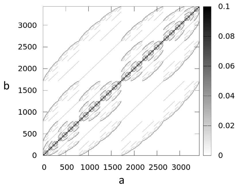
Figure 1: Rendering of $|h_{ab}|$ as function of the compressed indices $(a,b)$ for the Hubbard-type model (83) with $t_{ij}=e^{-0.2|i-j|}$, $u_{ij}=0.3e^{-0.5|i-j|}$ and $\epsilon_{i}=0$. The plot was generated with (85), where the parameters were fixed at $q=14$ and $N=7$, in which case the dimension of the $N$-particle sector was $D_{N}=3432$.

Computer Code 4

We provide here code lines which compute and store the matrix of the Hamiltonian defined in Example 2, this time in the $N$-th particle sector of $\mathcal{M}_{2^{q}}$.

$$\boxed{\begin{array}[]{l}\mathrm{input}\ N\\ \mbox{Call Eq.~{}\eqref{Eq:IndN}}\\ h_{a,b}=0,\ a,b=1,\ldots,D_{N}\\ \mathrm{do}\ n=0,2^{q}-1\\ \ \ \mbox{Call Eq.~{}\ref{Binary}}\\ \ \ \mathrm{if}(\mathrm{sum}(\mathfrak{b}_{n})=N)\ \mathrm{then}\\ \ \ \ \ \mathrm{do}\ i=0,q-1\\ \ \ \ \ \ \ \mathrm{do}\ j=0,q-1\\ \ \ \ \ \ \ \ \ \mathrm{if}(\mathfrak{b}_{n}(i)=1\ \&\ \mathfrak{b}_{n}(j)=0)\ \mathrm{then}\\ \ \ \ \ \ \ \ \ \ \ \mathcal{N}_{ij}=\mathrm{sum}\big{(}\mathfrak{b}_{n}(\min(i,j):\max(i,j))\big{)}\\ \ \ \ \ \ \ \ \ \ \ a=\mathrm{ind}(n);b=\mathrm{ind}(n-2^{i}+2^{j})\\ \ \ \ \ \ \ \ \ \ \ h_{a,b}=h_{a,b}-(-1)^{\mathcal{N}_{ij}}(1-\delta_{ij})t_{ij}\\ \ \ \ \ \ \ \ \ \ \ h_{b,a}=h_{b,a}-(-1)^{\mathcal{N}_{ij}}(1-\delta_{ij})\bar{t}_{ij}\\ \ \ \ \ \ \ \ \ \mbox{end if}\\ \ \ \ \ \ \ \ \ \mathrm{if}(\mathfrak{b}_{n}(i)=\mathfrak{b}_{n}(j)=1)\ \mathrm{then}\\ \ \ \ \ \ \ \ \ \ \ a=\mathrm{ind}(n)\\ \ \ \ \ \ \ \ \ \ \ h_{a,a}=h_{a,a}+\delta_{ij}\epsilon_{i}+u_{ij}\\ \ \ \ \ \ \ \ \ \mathrm{end\ if}\\ \ \ \ \ \ \ \mathrm{end\ do}\\ \ \ \ \ \mathrm{end\ do}\\ \ \ \mathrm{end\ if}\\ \mathrm{end\ do}\\ {\rm return}\ h_{a,b},\ a,b=1,\ldots D_{N}.\end{array}}$$ (85)

An output of this algorithm is illustrated in Fig. 1. $\Diamond$

VI Conclusions

Although the examples we provided were all 1-dimensional, our analysis covers quite generic settings because, once a basis for the one-particle Hilbert space is chosen, Hamiltonians are all rendered using linear indices. To exemplify this point, let us consider a 2-dimensional $L\times L$ lattice $\mathcal{L}_{L}=\mathbb{Z}_{L}\times\mathbb{Z}_{L}$ ($\mathbb{Z}_{L}=\mathbb{Z}/L\mathbb{Z}$) with $K$ quantum states per site, as well as a generic Hubbard-type Hamiltonian:

$$H=\sum_{\bm{i},\bm{j}\in\mathcal{L}_{L}}\sum_{\alpha,\beta=0}^{K-1}\Big{[} (1-\delta_{\bm{i}\bm{j}}\delta_{\alpha\beta})\big{(}t_{\bm{i}\bm{j}}^{\alpha\beta}\,a_{\bm{i},\alpha}^{\ast}a_{\bm{j},\beta}+\bar{t}_{\bm{i}\bm{j}}^{\alpha\beta}\,a_{\bm{j},\beta}^{\ast}a_{\bm{i},\alpha}\big{)}$$ (86)

$$\quad+\big{(}\delta_{\bm{i}\bm{j}}\,\delta_{\alpha\beta}\epsilon_{\bm{i}}^{\alpha}+u_{\bm{i}\bm{j}}^{\alpha\beta}\big{)}\,n_{\bm{i},\alpha}\,n_{\bm{j},\beta}\Big{]},$$

This model can be reduced identically to the Hamiltonian in Eq. (66), by creating a linear index $i$ for the one-particle Hilbert space $\mathbb{C}^{K}\otimes\ell^{2}(\mathcal{L}_{L})$ of the model. One way to achieve that is by applying the rule:

$$\begin{array}[]{c}\mathcal{L}_{L}\times\mathbb{Z}_{K}\ni(\alpha,\bm{i})=(\alpha,i_{1},i_{2})\\ \Downarrow\\ i=\alpha+i_{1}\,K+i_{2}\,L\,K\in\mathbb{Z}_{q},\end{array}$$ (87)

with $q=K\,L^{2}$. Once we encode the information and re-write the Hamiltonian (86) using this linear index, which amounts to re-encoding the coefficients $t_{\bm{i}\bm{j}}^{\alpha\beta}\rightarrow t_{ij}$ and $u_{\bm{i}\bm{j}}^{\alpha\beta}\rightarrow u_{ij}$, there is nothing to be added to the previous analysis. Of course, not all basis set choices are the same and some can prove to be more optimal, in the sense that the coefficients $t_{ij}$ are of shorter-range. This is an important issue which needs to be solved before the matrix-representation is attempted.

We also want to stress that the calculations can be straightforwardly expanded to cover higher order products of generators. This becomes quite apparent if the reader examines Eq. 53 and the manipulations after it. Specific applications taking advantage of these matrix representations will be reported in a future work.

- [1] O. Bratteli, D. W. Robinson, Operator algebras and quantum statistical mechanics 2, (Springer, Berlin, 2002).
- [2] F. D. M. Haldane, The origin of holomorphic states in Landau levels from non-commutative geometry, and a new formula for their overlaps on the torus, J. Mathe. Phys. 59, 081901 (2018).
- [3] L. Fidkowski, A. Kitaev, Effects of interactions on the topological classification of free fermion systems, Phys. Rev. B 81, 134509 (2010).
- [4] Lukasz Fidkowski and Alexei Kitaev, Topological phases of fermions in one dimension, Phys. Rev. B 83, 075103 (2011).
- [5] E. Prodan, F.D.M. Haldane, Mapping the braiding properties of the Moore-Read state, Phys. Rev. B 80, 11512 (2009).
- [6] K. R. Davidson, -Algebras by Example, (AMS, Providence, 1996).
- [7] J. Renault, A groupoid approach to -algebras, (Springer-Verlag, Berlin, 1980).
- [8] E. G. Effros, Dimensions and -algebras, (AMS, Providence, 1981).