Navigating Around Convex Sets

Abstract

We review some basic results of convex analysis and geometry in $\mathbb{R}^{n}$ in the context of formulating a differential equation to track the distance between an observer flying outside a convex set $K$ and $K$ itself.

1 Introduction.

Suppose you fly by a convex body in $\mathbb{R}^{n}$. A fundamental problem in convex analysis is to determine your distance $r(t)$ to that body as you are flying. To the best of our knowledge, all standard algorithms to do this determine the point in the convex set nearest to you by optimization, at every point in time when needed or possible. In this exposition, we propose to solve the optimization problem only once, at $t=0$, say, and then track $r(t)$ by solving a differential equation for it. The study of this problem allows us to review some of the basic tenets of convex analysis.

Let $K$ be a closed (solid) convex body in $\mathbb{R}^{n}$ and denote by $\mathbb{R}^{n}\backslash K$ by $\Omega$. The fly-by curve in $\Omega$ is given by the trajectory $c(t)$, which we will always assume to be smooth. To find $r(t)$, we need to know the point in $K$ nearest to $c(t)$. This point is called the projection of $c(t)$ onto $K$ and will be denoted by $\Pi(c(t))$ or $\Pi(t)$ for short. If we hope to write down a differential equation for $r(t)$, we will at least have to know the one-sided derivative of $\Pi(c(t))$ with respect to time:

$$\Pi_{+}^{\prime}(t_{0})\equiv\,\lim_{t\searrow 0}\,\dfrac{\Pi(t)-\Pi(0)}{t}.$$ (1)

In Section 2 we give an elementary proof that if in $\mathbb{R}^{2}$, the boundary $\partial K$ of $K$ is twice differentiable, then this one-sided derivative exists. In Section 3, we will see that this derivative exists for any piecewise linear polygon. Then we will outline the construction from [3] of a convex body in $\mathbb{R}^{2}$ whose boundary is $C^{1,1}$ ($C^{1}$ with a Lipschitz derivative) but for which $\Pi_{+}^{\prime}$ does not exist (Theorem 1).

In Sections 4 and 5, the differential equations are constructed that allow us to continually monitor the distance $r(t)$ to a convex body as we navigate around it. The general case is not much different from $\mathbb{R}^{3}$, so for ease of exposition we stick to $\mathbb{R}^{3}$. The construction is straightforward and employs the Weingarten equations (or Ricci curvature) from differential geometry. To the best of our knowledge, the final form of these equations (Theorem 17) is new. We invoke the existence and uniqueness theorems for the solutions of differential equations to show that if the boundary of $K$ is $C^{2,1}$, then the system of differential equations has a unique solution. In Section 7, we give two examples of these equations and their solutions.

To the careful reader it will be clear that all we really need to formulate these differential equations are one-sided time derivatives (as in equation (1)). Thus if you fly near a convex body, you can change your course to another differentiable one, all the while continuing to monitor the distance. Thus the equations of Sections 4 and 5 can be used to avoid collision with a convex set. Hence our title. Even if $K$ is not convex, one could use these equations to avoid the convex hull of $K$.

Finally, in Section 6, we discuss the classical, but still remarkable, fact that the function $r:\Omega\rightarrow\mathbb{R}$ giving the distance of a point to the convex set is always differentiable (Theorem 3)! There is no regularity requirement at all on the convex set. Our exposition of this fact is inspired by [8].

The subject of distance to convex sets is much too rich to do justice to in this short introduction. But we do wish to point out a few directions in which considerable further research has been done. Our own interest (beside [3]) ultimately derives from a closely related problem, namely: Given a Riemannian manifold and two disjoint compact subsets $A$ and $B$, what are the topological [4, 18] and geometric [11] characteristics of the set of points whose distance to $A$ equals their distance to $B$? Beside their intrinsic interest, these sets have many applications among others in the study of Brillouin zones in quantum mechanics [19].

The distance function to $\partial K$ is not differentiable at $\partial K$. Indeed, at a point of $\partial K$, it behaves like the function $x\rightarrow|x|$ near 0. For this reason one is also interested [1] in the smoothness of the signed distance, which is negative on one side of the surface and positive on the other. This obviously only works for embedded codimension one surfaces. Thus for more generality, one also studies the properties of $r^{2}$. This is not formally a distance, but still closely related, and is differentiable at ${\partial K}$ (see [1]).

There are many generalizations of the regularity of the distance function. In a smooth Riemannian manifold, or Alexandrov space, the notion of convexity may not be well-defined. So, instead of the derivative of the distance $r(t)$ to a closed subset $K$, one looks instead at its one-sided derivative along a geodesic $c(t)$ with initial point $x_{0}\in\Omega$:

$$r_{+}^{\prime}(0)\equiv\,\lim_{t\searrow 0}\,\dfrac{r(c(t))-r(c(0))}{t}.$$ (2)

The generalization of Theorem 3 holds and states that this one-sided derivative always exists (see [15] and [5, Exercise 4.5.11]). Further differentiability beyond that depends on the smoothness of the subset $K$ (for example, [13, 14]). Other generalizations consider the distance to convex sets in Hilbert spaces (see [7, 17]).

2 Twice Differentiable Sets in $\mathbb{C}$.

It is convenient to use complex coordinates in $\mathbb{R}^{2}$. So, we identify $\mathbb{R}^{2}$ with $\mathbb{C}$. We will assume that the boundary $\partial K$ is a twice differentiable curve $z(s)$. We also assume that $z:\mathbb{R}\rightarrow\mathbb{C}$ is a unit speed parametrization, that is, $|z^{\prime}(s)|=1$. We orient the boundary $z(s)$ of $K$ counter-clockwise (see Figure 1).

The trajectory of a point outside the body $K$ depends on time and is given by

$$c=z-irz^{\prime}\quad\textrm{or}\quad c(t)=z(s(t))-ir(t)z^{\prime}(s(t)),$$ (3)

so that in $\Omega$ (outside the convex body), $r$ is positive. Note that we indicate differentiation with respect to time $t$ with a dot (for example, $\dot{c}(t)$), whereas differentiation with respect to the parameter of the convex body is indicated by an accent (for example, $z^{\prime}(s)$).

$$\dot{c}=(z^{\prime}-irz^{\prime\prime})\dot{s}-i\,\dot{r}z^{\prime}.$$ (4)

Now denote by $\dot{c}_{\|}$ and $\dot{c}_{\bot}$ the components of $\dot{c}$ parallel and orthogonal, respectively, to $z^{\prime}$ (derivative with respect to $s$). Since $|z^{\prime}(s)|=1$, we have that $z^{\prime\prime}(s)$ is orthogonal to $z^{\prime}(s)$, and thus $iz^{\prime\prime}(s)$ is parallel to $z^{\prime}$. Thus, equation (4) quite naturally splits into two components as described in the following lemma:

Lemma 1.

Suppose $z$ is twice differentiable and $c$ is a differentiable trajectory outside $K$. We have

$$\left\{\begin{array}[]{ccccc}\dot{s}&=&\dfrac{\dot{c}_{\|}}{z^{\prime}-irz^{\prime\prime}}&=&\textrm{Re}\left(\dfrac{\dot{c}}{z^{\prime}-irz^{\prime\prime}}\right)\\[9.95863pt] \dot{r}&=&\dfrac{i\dot{c}_{\bot}}{z^{\prime}}&=&\textrm{Re}\left(\dfrac{i\dot{c}}{z^{\prime}}\right)\\[5.69046pt] \end{array}\right.\quad.$$ (5)

Figure 1: In the left figure, $K$ has a nondifferentiable boundary, but the one-sided derivative of the projection still exists. In the right figure, $K$ has a twice differentiable boundary. The tangent vector $z^{\prime}(s)$ and the curvature vector $z^{\prime\prime}(s)$ are orthogonal, because $z$ is a unit speed parametrization.

Equation (3) implies that in the orientation of the parametrization sketched in Figure 1, $r(t)$ is positive. Thus $irz^{\prime\prime}$ is parallel to $z^{\prime}$, but actually points in the opposite direction. Because $z^{\prime}(s)\dot{s}$ is the derivative of the projection, equation (5) proves the following lemma. This result generalizes to higher dimension (see Corollary 1).

Lemma 2.

If $\partial K$ is twice differentiable, then $|\Pi_{+}^{\prime}(0)|=\dfrac{|\dot{c}_{\|}|}{1+r\,|z^{\prime\prime}|}$ ($r>0$ in $\Omega$).

3 A $C^{1,1}$ Counterexample.

If we drop the requirement that $z(s)$ is twice differentiable, a set can be constructed where $\Pi_{+}^{\prime}(0)$ does not exist. We now give that construction, and outline the reason it works. Our treatment is loosely based on [3], which contains the full details.

One might be tempted to say that, of course, $z$ must be differentiable for $\Pi_{+}^{\prime}$ to exist. But that would be wrong! Consider the set up on the left side of Figure 1, where $c(t)$ is a straight line ($c^{\prime}(t)$ is constant). Consider the (shaded) cone in $\Omega$ formed by the perpendiculars to the tangents of the surface at the nondifferentiable point. Before reaching the cone, $\Pi_{+}^{\prime}(t)$ is a constant determined by the angle between $c^{\prime}(t)$ and the left flank of $\partial K$. As soon as $c$ hits the left boundary of the cone, $\Pi_{+}^{\prime}(t)=0$ because we are looking at the one-sided derivative (see equation (1)). Again, when $c$ hits the right boundary of the cone, the one-sided derivative is a nonzero constant. Clearly, the one-sided derivative exists for every piecewise linear polygon. In the light of this, it becomes nontrivial to find a counterexample to the existence of the one-sided derivative of the projection. A beautiful and surprisingly simple example of a nonempty closed continuous convex set for which the directional derivative of the metric projection mapping fails to exist was constructed by Shapiro in [16] and fine-tuned in [3] to become $C^{1,1}$.

For some $\lambda\in(0,1)$, define a sequence of real numbers $\{\alpha_{n}\}_{n\in\mathbb{N}}\subset(0,\pi]$ by

$$\alpha_{n}=C\lambda^{n}\quad\textrm{and set }\quad A_{n}=e^{i\alpha_{n}}.$$ (6)

($C$ is any positive real so that $\alpha_{n}\in(0,\pi]$ for all $n$.) This set in [16] is the convex hull of the collection of points $0$, $1$, and $\{A_{n}\}_{n\in\mathbb{N}}$. See the left part of Figure 2.

The right part of Figure 2 shows the figure modified by the techniques of [3], which is now $C^{1,1}$. The construction is as follows. Let $T_{n}$ be the midpoint of the line segment $A_{n}A_{n+1}$ and let $S_{n}$ be the point in the line segment $A_{n-1}A_{n}$ such that

$$\textrm{length}(T_{n}A_{n})=\textrm{length}(A_{n}S_{n}).$$

Replace the two line segments $T_{n}A_{n}$ and $A_{n}S_{n}$ by a circular arc $C_{n}$ tangent to both segments. Define the convex set $K$ as the convex hull of all arcs $C_{n}$ and the arc of the unit circle in the lower half-plane connecting $1$ and $A_{1}$. Clearly, the boundary of $K$ is differentiable, except at $A_{1}$. This is easily remedied, but, since it is irrelevant for the remainder, we omit the details.

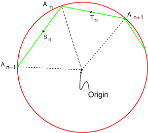
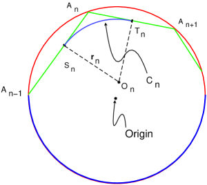
Figure 2: On the left, the $C^{0}$ counterexample given by Shapiro, and on the right its modification into a $C^{1,1}$ set. For clarity, the drawing is not on a realistic scale.

To continue, we first mention a curious result. The radius of curvature of the arcs $C_{n}$ is denoted by $r_{n}$ (see Figure 2). The radius of curvature by definition equals $1/|z^{\prime\prime}(s)|$. The following lemma can be shown by any persistent reader, since it uses only elementary planar geometry. We omit the proof.

Lemma 3.

In the modified construction, $\lim_{n\rightarrow\infty}\,r_{n}$ exists and is equal to $r_{\infty}=\dfrac{2\lambda}{1+\lambda}$.

Let $c(t)=2e^{it/2}$, the unit speed curve along the radius 2 circle centered at the origin. Near $t=0$, we see that $|\dot{c}_{\|}|=1$ and $|\dot{c}_{\perp}|=0$. On the curve $c$, mark the times where $\Pi(t)=\Pi(c(t))$ equals $T_{n}$ by $t_{n}$, and times where $\Pi(t)$ equals $S_{n}$ by $s_{n}$ (see Figure 3). Again, using elementary planar geometry, the avid reader can prove the following lemma.

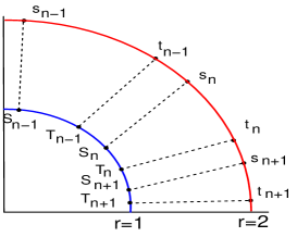
Figure 3: The unit speed orbit $c(t)$ winds around the radius 2 circle. At times $t_{n}$, its projection is $T_{n}$, and at times $s_{n}$, its projection is $S_{n}$.

Lemma 4.

In the modified construction, the following limits exist:

$$p_{\infty}:=\lim_{n\rightarrow\infty}\,\frac{t_{n-1}-s_{n}}{t_{n-1}}\quad\textrm{and}\quad q_{\infty}:=\lim_{n\rightarrow\infty}\,\frac{s_{n}-t_{n}}{s_{n}},$$

and both are in $(0,1)$.

Theorem 1.

The modified construction just described yields a differentiable curve $z(s)$ for the boundary of $K$ and $z^{\prime}(s)$ is uniformly Lipschitz. The projection $\Pi$ onto this set does not have a directional derivative at $z=1$.

The remainder of this section is a sketch of the proof of Theorem 1.

Proof.

We first establish that the curve is differentiable and its derivative is uniformly Lipschitz. By construction, $\partial K$ consists of circular arcs $C_{n}$ (and a part of the unit circle), and straight segments $T_{n-1}S_{n}$. So it is clear that $\partial K$ is $C^{1}$ and $C^{2}$ almost everywhere. Where a segment and an arc are glued together, the derivative of $z$ is a continuous function which is constant on one side and has constant slope on the other. By Lemma 3, this slope is bounded, and so the derivative is uniformly Lipschitz.

The only problematic point is $z=1$ where the arcs $C_{n}$ accumulate. On the one hand, the line $\ell=\{1+it\,|\,t\in\mathbb{R}\}$ intersects $\partial K$ only at $z=1$. The points $1$ and $T_{n}$ are contained in $K$. By convexity, the chords from $1$ to $T_{n}$ are contained in $K$. The slope of these chords accumulate to the slope of $\ell$. Hence, $\ell$ is the tangent line at $z=1$. This establishes differentiability. With a little extra effort, the argument in the previous paragraph also applies to $z=1$, establishing the Lipschitz condition there.

We next establish that the directional derivative of equation (1) does not exist near $z=1$. If $t\in(t_{n},s_{n+1})$, then $\Pi(t)$ is part of a segment, and if $t\in(s_{n},t_{n})$, then by $\Pi(t)$ is in $C_{n}$. Lemma 2 and Lemma 3 imply that for $n$ large (or $t$ near 0)

$$\begin{array}[]{ccl}\textrm{if }t\in(t_{n-1},s_{n})&\textrm{ then }&|\Pi^{\prime}(t)|=1\quad\textrm{ and}\\ \textrm{if }t\in(s_{n},t_{n})&\textrm{ then }&|\Pi^{\prime}(t)|=\dfrac{r_{n}}{1+r_{n}}\rightarrow\dfrac{2\lambda}{1+3\lambda}<\dfrac{2}{3}.\end{array}$$ (7)

This leads to the following equality:

$$\dfrac{\Pi(t_{n-1})-\Pi(0)}{t_{n-1}}=\dfrac{\Pi(t_{n-1})-\Pi(s_{n})}{t_{n-1}-s_{n}}\,\dfrac{t_{n-1}-s_{n}}{t_{n-1}}+\dfrac{\Pi(s_{n})-\Pi(0)}{s_{n}}\,\dfrac{s_{n}}{t_{n-1}}.$$ (8)

Now if we assume that the one-sided directional derivative exists and insert equation (7) and $p_{\infty}$ defined in Lemma 4 into the previous equation, then, as $n$ tends to infinity, we obtain

$$\Pi_{+}^{\prime}(0)=1\cdot p_{\infty}+\Pi_{+}^{\prime}(0)(1-p_{\infty})\quad\textrm{or}\quad(\Pi_{+}^{\prime}(0)-1)p_{\infty}=0.$$

It follows that $\Pi_{+}^{\prime}(0)=1$ or that $p_{\infty}=0$. The latter is impossible by Lemma 4. Similarly, the equality

$$\dfrac{\Pi(s_{n})-\Pi(0)}{s_{n}}=\dfrac{\Pi(s_{n})-\Pi(t_{n})}{s_{n}-t_{n}}\,\dfrac{s_{n}-t_{n}}{s_{n}}+\dfrac{\Pi(t_{n})-\Pi(0)}{t_{n}}\,\dfrac{t_{n}}{s_{n}},$$ (9)

under the hypothesis that $\Pi_{+}^{\prime}(0)$ exists, leads to the conclusion that $\Pi_{+}^{\prime}(0)<\frac{2}{3}$. Thus we have a contradiction and, hence, $\Pi_{+}^{\prime}(0)$ cannot exist. ∎

There are two open questions related to this construction that are perhaps worth mentioning. The first is: Can this construction be modified to obtain a curve $z(s)$ so that the quantity $\Pi_{+}^{\prime}$ fails to exist in a set of points that is dense in some open subset of $\Omega$? The second question is: Is there a $C^{2}$ curve $\boldsymbol{\sigma}(u)$ in $\mathbb{R}^{2}$ for which the solution of equation (14) is not unique? For such a curve, the one-sided derivative of the projection does exist by Lemma 1. But the solution of the differential equation would not be unique.

4 Twice Differentiable Sets in $\mathbb{R}^{2}$.

For the next two sections, we return to the smooth (at least $C^{2}$) case. It is interesting to translate the considerations in Section 2 to the vector space $\mathbb{R}^{n}$. For simplicity, we start with $\mathbb{R}^{2}$.

Recall that $z:\mathbb{R}\rightarrow\mathbb{R}^{2}$ given by $\boldsymbol{\sigma}(u)$ is the unit speed anti-clockwise parametrization of the boundary of the convex body. Denote its unit tangent vector by ${\boldsymbol{\sigma}}^{\prime}$, and $\bf n$ is the unit vector normal to it, pointed into the body (to get a right-handed coordinate system $({\boldsymbol{\sigma}}^{\prime},\bf n)$). Note that $iz^{\prime}$ in the complex notation becomes ${\bf n}$, and that the complex $z^{\prime\prime}$ becomes $\kappa{\bf n}$. The sign of $\kappa$ — nonnegative here — is determined by the convexity of the body. We now give the translations of equations (3) through (5) to $\mathbb{R}^{2}$.

The position $c$ of a point outside the body is given by

$$c=\boldsymbol{\sigma}(u)-r{\bf n}.$$ (10)

(Note that $r$ is positive in $\Omega$.) Now let $c(t)$ be a smooth curve. Differentiating with respect to $t$ while noting that $\dot{\boldsymbol{n}}=-\kappa{\boldsymbol{\sigma}}^{\prime}$, gives

$$\dot{c}={\boldsymbol{\sigma}}^{\prime}(1+r\kappa)\dot{u}-{\bf n}\dot{r}.$$ (11)

To write this in matrix form, define the matrix $\Sigma$ as having its first column equal to ${\boldsymbol{\sigma}}^{\prime}$ and its second equal to ${\bf n}$. Then

$$\dot{c}=\Sigma\begin{pmatrix}1+r\kappa&0\\ 0&-1\end{pmatrix}\begin{pmatrix}\dot{u}\\ \dot{r}\end{pmatrix}.$$ (12)

Now $\Sigma$ is a unitary matrix (in fact, orthogonal) and so

$$\begin{pmatrix}\dot{u}\\ \dot{r}\end{pmatrix}=\begin{pmatrix}(1+r\kappa)^{-1}&0\\ 0&-1\end{pmatrix}\,\Sigma^{T}\,\dot{c}.$$ (13)

Inverting the matrices gives us the next lemma.

Lemma 5.

Suppose $\boldsymbol{\sigma}$ is twice differentiable and $c$ is a differentiable trajectory outside $K$. We have

$$\left\{\begin{array}[]{ccc}\dot{u}&=&\dfrac{{\boldsymbol{\sigma}}^{\prime}(u)\cdot\dot{c}}{1+r\kappa(u)}\\[9.95863pt] \dot{r}&=&-{\boldsymbol{n}}(u)\cdot\dot{c}\end{array}\right.\quad,$$ (14)

where $x\cdot y$ refers to the standard inner product in $\mathbb{R}^{2}$.

In practice, the unit speed parametrization is not so useful, since for most curves (including ellipses) explicit forms of such parametrizations are difficult or impossible find [10]. The method we use in Section 5 will avoid this problem altogether. For now, as a very simple illustration, consider the case where $K$ is the unit disk. Its circumference is parametrized by ${\boldsymbol{\sigma}}(u)=(\cos u,\sin u)$. The radius of curvature equals 1. Suppose $c=(x(t),y(t)$; then in this case the equations become

$$\left\{\begin{array}[]{ccc}\dot{u}&=&\dfrac{-\dot{x}\sin u+\dot{y}\cos u}{1+r}\\[9.95863pt] \dot{r}&=&\dot{x}\cos u+\dot{y}\sin u\end{array}\right..$$ (15)

We will look at more complicated examples in Section 7.

The assumption that $\boldsymbol{\sigma}(u)$ is $C^{2}$ is essential here. The example of Section 3 shows that $\dot{u}$ may not exist if the boundary is $C^{1,1}$. The same holds in higher dimension (see Section 5), though we will not repeat this observation.

5 Twice Differentiable Sets in $\mathbb{R}^{3}$.

In three dimensions, these equations become much more interesting. The generalization from there to $\mathbb{R}^{n}$ is easy to guess; one needs to replace the matrix $W$ below with the $n-1$ by $n-1$ Ricci curvature tensor of the hypersurface. We will stick to $\mathbb{R}^{3}$ for simplicity.

Let ${\boldsymbol{\sigma}}(u,v)$ be a smooth (at least $C^{2}$) parametrization of a surface in $\mathbb{R}^{3}$ bounding a convex body $K$. Denote ${\partial_{u}\boldsymbol{\sigma}}$ by $\boldsymbol{\sigma}_{u}$ and ${\partial_{v}\boldsymbol{\sigma}}$ by $\boldsymbol{\sigma}_{v}$. To get a right-handed coordinate system $({\boldsymbol{\sigma}}_{u},{\boldsymbol{\sigma}}_{v},{\bf n})$, we define the unit normal ${\bf n}$:

$${\bf n}=\dfrac{{\boldsymbol{\sigma}}_{u}\times{\boldsymbol{\sigma}}_{v}}{{|\boldsymbol{\sigma}}_{u}\times{\boldsymbol{\sigma}}_{v}|}.$$

To connect with the earlier sections, we will set things up in such a way that ${\bf n}$ points into the convex body $K$. Let $\Sigma$ be the invertible $3\times 3$ matrix whose first column is $\boldsymbol{\sigma}_{u}$, whose second column is $\boldsymbol{\sigma}_{v}$, and whose third is ${\bf n}$. Note that the above assumptions imply that the determinant of this matrix is positive. Furthermore, let $W$ be the $2\times 2$ Weingarten matrix, that is (see [6]),

$$\left\{\begin{array}[]{ccc}{\bf n}_{u}&=&a{\boldsymbol{\sigma}}_{u}+b{\boldsymbol{\sigma}}_{v}\\[9.95863pt] {\bf n}_{v}&=&c{\boldsymbol{\sigma}}_{u}+d{\boldsymbol{\sigma}}_{v}\\[9.95863pt] \end{array}\right.\quad\textrm{where}\quad\begin{pmatrix}a&c\\ b&d\end{pmatrix}=W.$$ (16)

The eigenvalues of $-W$ are the principal curvatures of the surface (see [6]). By convexity — recall that ${\bf n}$ points away from $\Omega$ — these eigenvalues are nonnegative.

Theorem 2.

Suppose the parametrization $\boldsymbol{\sigma}$ of the boundary of $K$ is twice differentiable and $c$ is a differentiable trajectory outside $K$. Let $I$ be the $2\times 2$ identity matrix. We have

$$\begin{pmatrix}\dot{u}\\ \dot{v}\\ \dot{r}\end{pmatrix}=\begin{pmatrix}(I-rW)^{-1}&\vline&0\\ \hline\cr 0&\vline&-1\end{pmatrix}\,\Sigma^{-1}\,\dot{c}.$$ (17)

Proof.

Coordinatize $\Omega$, the space outside the convex body, as follows (see equation (10)):

$$P:=(u,v,r)\rightarrow{\boldsymbol{\sigma}}(u,v)-r{\bf n},$$

where $r>0$ in $\Omega$. Let $c(t):=(u(t),v(t),r(t))$ be a smooth curve in $\Omega$, then

$$\begin{array}[]{ccl}\dot{c}&=&{\boldsymbol{\sigma}}_{u}\dot{u}+{\boldsymbol{\sigma}}_{v}\dot{v}-{\bf n}\dot{r}-r{\bf n}_{u}\dot{u}-r{\bf n}_{v}\dot{v}\\[5.69046pt] &=&{\boldsymbol{\sigma}}_{u}((1-ra)\dot{u}-rc\dot{v})+{\boldsymbol{\sigma}}_{v}(-rb\dot{u}+(1-rd)\dot{v})-{\bf n}\dot{r},\end{array}$$

where we have used equation (16). In matrix form, this gives

$$\dot{c}=\Sigma\,\begin{pmatrix}I-rW&\vline&0\\ \hline\cr 0&\vline&-1\end{pmatrix}\begin{pmatrix}\dot{u}\\ \dot{v}\\ \dot{r}\end{pmatrix}.$$

Since the eigenvalues of $-W$ are nonnegative and $r$ is positive in $\Omega$, this relation can be inverted to yield the theorem. ∎

Given the vector $\dot{c}$ of the trajectory of the observer, the derivative of the projection is given by ${\boldsymbol{\sigma}}_{u}\dot{u}+{\boldsymbol{\sigma}}_{v}\dot{v}$. Thus equation (17) implies the following.

Corollary 1.

If the surface in $\mathbb{R}^{3}$ is twice differentiable, then the directional derivative exists.

For existence and uniqueness of the solution of this differential equation, the conditions of Theorem 17 are insufficient. We need to require that the right-hand side is Lipschitz in $(u,v,r)$ and continuous in $t$ (see [12]).

Corollary 2.

(Local) existence and uniqueness of the solution of differential equation (17) is guaranteed if $W$ is Lipschitz and $c$ is continuously differentiable.

Proof.

The continuity in $t$ of the right-hand side of equation (17) is guaranteed by the smoothness of $c$. We now check the Lipschitz condition in $(u,v,r)$. Lipschitz in $r$ is straightforward. Since ${\boldsymbol{\sigma}}$ is $C^{2}$, $\Sigma$ is differentiable and invertible, and therefore so is $\Sigma^{-1}$. Hence, $\Sigma^{-1}$ is certainly Lipschitz. The question then is whether $(I-rW)^{-1}$ is Lipschitz. The following computation shows that if $W$ is Lipschitz, then so is $(I-rW)^{-1}$.

From the previous discussion, we are allowed to hold $r$ constant. Let us denote the operator norm by $\|\cdot\|$ and set $x=(u,v)$. Then

$$\begin{array}[]{l}\|(I-rW(x_{2}))^{-1}-(I-rW(x_{1}))^{-1}\|\\ \hskip 36.135pt=|(I-rW(x_{2}))^{-1}\left[r(W(x_{2})-W(x_{1})\right](I-rW(x_{1}))^{-1}|\\ \hskip 36.135pt\leq r\|(I-rW(x_{2}))^{-1}\|\|W(x_{2})-W(x_{1})\|\|(I-rW(x_{1}))^{-1}\|.\end{array}$$

The first and last term are at most 1 by convexity (the eigenvalues of $W$ are nonpositive). The middle term is Lipschitz by assumption. ∎

If we want the solution of equation (17) to depend differentiably on time and initial conditions, we need to require even more.

Proposition 1.

Let $\phi(t,u_{0},v_{0},r_{0})$ be the solution of equation (17) with initial condition $(u_{0},v_{0},r_{0})$ at $t=0$. Let $p\geq 1$ an integer. If $c(t)$ is $C^{p+1}$ and ${\boldsymbol{\sigma}}(u,v)$ is $C^{p+2}$, then $\phi$ is $C^{p}$ in $(t,u_{0},v_{0},r_{0})$.

Proof.

In [2, Chapter 32], it is proved that if $\dot{x}=f(t,x)$ and $f$ is $C^{p}$ for some integer $p\geq 1$, then the initial value problem is also $C^{p}$. Inspection of equation (17) shows that the conditions of the proposition are sufficient to guarantee that its right-hand side is $C^{p}$. ∎

6 Differentiability of the Distance Function.

If we restrict ourselves to the distance function, we can do much better for its regularity than the results in Section 5. In this section, we assume that $K$ is closed and convex, but make no further regularity assumption.

Lemma 6.

Suppose that $x_{i}$ is in $\Omega$ and $\lim x_{i}=x_{\infty}$. Let $y_{i}\in\Pi(x_{i})$. Then any convergent subsequence of $\{y_{i}\}$ converges to a point $y_{\infty}$ in $\Pi(x_{\infty})$.

Proof.

Suppose the opposite; then pick a subsequence of the $i$ so that $\{y_{i}\}$ is convergent to a point $y_{\infty}$ that is not in $\Pi(x_{\infty})$. Let $y\in\Pi(x_{\infty})$; then for some positive $\Delta$, we have $d(x_{\infty},y_{\infty})=d(x_{\infty},y)+\Delta$. Now take $\epsilon$ arbitrarily small. Using the triangle inequality, we see that for $n$ large enough $d(x_{\infty},x_{n})+d(x_{n},y_{n})+d(y_{n},y_{\infty})\geq d(x_{\infty},y_{\infty})$, and so

$$d(x_{n},y_{n})\geq d(x_{\infty},y_{\infty})-d(x_{\infty},x_{n})-d(y_{n},y_{\infty})\geq d(x_{\infty},y)+\Delta-2\epsilon.$$

On the other hand, using the triangle inequality for large $n$ again,

$$d(x_{n},y)\leq d(x_{\infty},y)+d(x_{n},x_{\infty})<d(x_{\infty},y)+\epsilon.$$

Taking the two together, we get that $d(x_{n},y_{n})>d(x_{n},y)$, which contradicts the fact that $y_{n}$ minimizes the distance from $x_{n}$ to $K$. ∎

If $K$ is convex, then $\Pi(x_{\infty})$ is a single point $y$. Thus every convergent subsequence of $\{y_{i}\}$ in the Lemma 6 must converge to that point. Since the $\{y_{i}\}$ are confined to a bounded portion of a closed set, they always have a convergent subsequence. Thus we have proved a nice corollary:

Corollary 3.

The projection $\Pi:\Omega\rightarrow K$ is continuous.

For the remainder of this section, denote by $\boldsymbol{\theta}$ the unit vector in the direction of $x-\Pi(x)$.

Lemma 7.

For any $x\in\Omega$ and any vector ${\bf v}$, we have

$$d(x+t{\bf v},\Pi(x))-d(x,\Pi(x))=t\boldsymbol{\theta}\cdot{\bf v}+o(t).$$

Proof.

The difference between the squares of the distances can be written using the standard inner product of $\mathbb{R}^{n}$:

$$d(x+t{\bf v},\Pi(x))^{2}-d(x,\Pi(x))^{2}=2t[x-\Pi(x)]\cdot{\bf v}+t^{2}|{\bf v}|^{2}.$$

The left-hand side factors, so that we can divide by $d(x+t{\bf v},\Pi(x))+d(x,\Pi(x))\sim 2|x-\Pi(x)|$, from which the lemma follows easily. ∎

Lemma 8.

For any $x\in\Omega$ and any vector ${\bf v}$, we have

$$\begin{array}[]{l}d(x+t{\bf v},\Pi(x+t{\bf v}))-d(x,\Pi(x+t{\bf v}))\\ \hskip 36.135pt=t\boldsymbol{\theta}\cdot{\bf v}+t\dfrac{\left[\Pi(x)-\Pi(x+t{\bf v})\right]}{|x-\Pi(x)|}\cdot{\bf v}+o(t).\end{array}$$

Proof.

The computation is essentially the same as that in the proof of Lemma 7.

$$\begin{array}[]{l}\hskip-21.68121ptd(x+t{\bf v},\Pi(x+t{\bf v}))^{2}-d(x,\Pi(x+t{\bf v}))^{2}\\[2.84544pt] \hskip 21.68121pt=2t[x-\Pi(x+t{\bf v})]\cdot{\bf v}+t^{2}|{\bf v}|^{2}\\[2.84544pt] \hskip 21.68121pt=2t[x-\Pi(x)]\cdot{\bf v}+2t[\Pi(x)-\Pi(x+t{\bf v})]\cdot{\bf v}+t^{2}|{\bf v}|^{2}.\end{array}$$ (18)

As before, we divide by $d(x+t{\bf v},\Pi(x))+d(x,\Pi(x))\sim 2|x-\Pi(x)|$. ∎

In our case where $K$ is convex, Corollary 3 implies the second term in the right-hand side of the statement of Lemma 8 is also $o(t)$. This is important in the following theorem. (An altogether different proof of Theorem 3 can be found in [9, Chapter 2].)

Theorem 3.

For any $x\in\Omega$ and any vector ${\bf v}$, we have

$$d(x+t{\bf v},\Pi(x+t{\bf v}))-d(x,\Pi(x))=t\boldsymbol{\theta}\cdot{\bf v}+o(t).$$

In other words, the distance function to a convex set in $\mathbb{R}^{n}$ is differentiable on $\Omega$.

Proof.

We note that by definition of the projection $\Pi$, we have

$$d(x+t{\bf v},\Pi(x+t{\bf v}))-d(x,\Pi(x))\leq d(x+t{\bf v},\Pi(x))-d(x,\Pi(x)).$$

And thus by Lemma 7,

$$d(x+t{\bf v},\Pi(x+t{\bf v}))-d(x,\Pi(x))\leq t{\boldsymbol{\theta}}\cdot{\bf v}+o(t).$$

Similarly, if we use Lemma 8 and Corollary 3 to make sure that $t|\Pi(x)-\Pi(x+t{\bf v})|=o(t)$, we obtain the reverse inequality

$$d(x,\Pi(x))\leq d(x,\Pi(x+t{\bf v}))=d(x+t{\bf v},\Pi(x+t{\bf v}))-t{\boldsymbol{\theta}}\cdot{\bf v}+o(t).$$

∎

It turns out Lemma 7 actually holds not just in $\mathbb{R}^{n}$ but in any Riemannian manifold (see [15]). The proof we gave of Lemma 8 is valid only in $\mathbb{R}^{n}$. The proof of Theorem 3 is a modified version of the proof that appeared in [8]. However, Theorem 3 also holds for Alexandrov spaces (a generalization of Riemannian manifolds) with nonpositive or nonnegative curvature, according to [5, Exercise 4.5.11].

7 Examples.

We close with a simple illustration of the equations discussed in Section 5. The situation is sketched in Figure 4. This example also illustrates the fact that straight lines in $\Omega$ do not generally project to geodesics on the surface.

Let $\sigma$ be the embedding of the cylinder of radius $\kappa^{-1}$ in $\mathbb{R}^{3}$. We choose a parametrization so that its orientation is consistent with that of the previous sections.

$${\boldsymbol{\sigma}}:(u,v)\rightarrow(\kappa^{-1}\cos v,\kappa^{-1}\sin v,u).$$

For positive constants $a$ and $b$ let the trajectory $c(t)$ be given by

$$c(t)=(t,b+\kappa^{-1},at).$$

Figure 4: On the left, the projection onto the $xy$-plane of the cylinder $C$ and the path $c$. On the right, the projection onto the $xz$-plane.

In the notation of Section 5, we calculate the matrix $\Sigma$ (whose first column is $\boldsymbol{\sigma}_{u}$, the second, $\boldsymbol{\sigma}_{v}$, and the third, ${\bf n}$).

$$\Sigma=\begin{pmatrix}0&-\kappa^{-1}\sin v&-\cos v\\ 0&\kappa^{-1}\cos v&-\sin v\\ 1&0&0\end{pmatrix}\quad\Longrightarrow\quad\Sigma^{-1}=\begin{pmatrix}0&0&1\\ -\kappa\sin v&\kappa\cos v&0\\ -\cos v&-\sin v&0\end{pmatrix}.$$

The Weingarten matrix $W$ is computed as in equation (16):

$$W=\begin{pmatrix}0&0\\ 0&-\kappa\end{pmatrix}\quad\Longrightarrow\quad(I-rW)^{-1}=\begin{pmatrix}1&0\\ 0&(1+\kappa r)^{-1}\end{pmatrix}.$$

The projection of $c(t)$ onto the cylinder together with its distance to the cylinder is thus given by the solution of equation (17), together with initial conditions. Noting that $\dot{c}=(1,0,a)$, these equations simplify to

$$\begin{array}[]{ccl}\dot{u}&=&a\\[2.84544pt] \dot{v}&=&\dfrac{-\kappa\sin v}{1+\kappa r}\\[2.84544pt] \dot{r}&=&\cos v\end{array}\quad\textrm{where}\quad\begin{array}[]{ccl}u(0)&=&0\\[2.84544pt] v(0)&=&\frac{\pi}{2}\\[2.84544pt] r(0)&=&b\end{array}.$$

This somewhat obscure-looking nonlinear system nonetheless has a simple solution. Due to the translational symmetry, the segment from $c(t)$ to its projection lies in the plane parallel to the $xy$-plane. Thus the distance $r(t)$ and the angle $v(t)$ can be found by inspection of Figure 4 on the left. We get

$$\begin{array}[]{ccl}u(t)&=&at\\[2.84544pt] v(t)&=&\arccos\dfrac{t}{\sqrt{\ell^{2}+t^{2}}}\\[2.84544pt] r(t)&=&\sqrt{\ell^{2}+t^{2}}-\kappa^{-1}\end{array},$$

where we have set $\ell\equiv\kappa^{-1}+b$. By inverting the second of these, we obtain its inverse $t(v)=\ell(\tan v)^{-1}=-\ell\tan(v+\frac{\pi}{2})$. In the $vu$-plane, this solution is therefore a reparametrization of the curve $(v,-a\ell\tan(v+\frac{\pi}{2}))$. We have drawn this curve and the curve $(t,r(t))$ for $t\in[-20,20]$ in Figure 5.

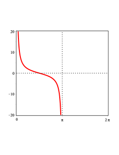
Figure 5: On the left, the projection of the trajectory $C:t\rightarrow(t,2,t)$ onto the cylinder $C:(u,v)\rightarrow(\cos v,\sin v,u)$. Horizontal is $v$, vertical is $u$. On the right, the distance $r(t)$ between $c(t)$ and its projection onto the cylinder $C$. Horizontal is $t$, vertical is $r$.

We now turn to a slightly more challenging example. This time $\boldsymbol{\sigma}$ is the embedding of the ellipsoid of revolution in $\mathbb{R}^{3}$. We choose a parametrization so that its orientation is consistent with that of the previous sections. This includes making sure that the normal is pointing into the surface.

$${\boldsymbol{\sigma}}:(u,v)\rightarrow(\cos u\sin v,\sin u\sin v,\kappa^{-1/2}\cos v).$$

Thus when $\kappa\in(0,1)$, the ellipsoid looks a little like a cigar, as in Figure 6, and when $\kappa\in(1,\infty)$, the ellipsoid is a flattened one.

Figure 6: An ellipsoid of revolution in spherical coordinates. Here, $u$ is the angle with the axis of the “north pole” and $v$ is the angle in the $xy$ plane with the positive $x$ axis.

With the same conventions as before, and following exactly the same procedure, we compute the matrix $S$ of tangent vectors and the Weingarten matrix $W$:

$$\Sigma=\begin{pmatrix}-\sin u\sin v&\cos u\cos v&{\dfrac{-\cos u\sin v}{\sqrt{1+(\kappa-1)\cos^{2}v}}}\\[11.38092pt] \cos u\sin v&\sin u\cos v&{\dfrac{-\sin u\sin v}{\sqrt{1+(\kappa-1)\cos^{2}v}}}\\[11.38092pt] 0&\dfrac{-\sin v}{\sqrt{\kappa}}&{\dfrac{-\sqrt{\kappa}\cos v}{\sqrt{1+(\kappa-1)\cos^{2}v}}}\end{pmatrix};$$

$$W=\begin{pmatrix}\dfrac{-1}{\left(1+(\kappa-1)\cos^{2}v\right)^{1/2}}&0\\ 0&\dfrac{-\kappa}{\left(1+(\kappa-1)\cos^{2}v\right)^{3/2}}\end{pmatrix}.$$

After setting

$$\begin{array}[]{ccl}q_{1}&=&\sqrt{1+(\kappa-1)\cos^{2}v}\end{array},$$

and some algebra, the equations of motion (17) become:

$$\begin{array}[]{ccl}\dot{u}&=&\dfrac{q_{1}}{(r+q_{1})\sin v}\;(-\dot{x}\,\sin u+\dot{y}\,\cos u)\\[11.38092pt] \dot{v}&=&\dfrac{q_{1}\,\kappa}{r\kappa+q_{1}^{3}}\;(\dot{x}\,\cos u\cos v+\dot{y}\,\sin u\cos v-\dot{z}\,\kappa^{-1/2}\sin v)\\[11.38092pt] \dot{r}&=&\dfrac{1}{q_{1}}\;(\dot{x}\cos u\sin v+\dot{y}\sin u\sin v+\dot{z}\sqrt{\kappa}\cos v)\end{array}.$$ (19)

Here $c(t)=(x(t),y(t),z(t))$ is the a priori given trajectory.

As an example, we set $\kappa=1/9$ and $c(t)=(2,t,t)$ and numerically solved equation (19) setting the initial condition $(u(0),v(0),r(0))=(0,\pi/2,1)$ and $(\dot{x},\dot{y},\dot{z})=(0,1,1)$. The results are displayed in Figure 7. The figure on the left shows the orbit of the projection $\Pi(c(t))$ for $t\in[0,100]$ (the continuous curve) and the orbit $c(t)$ (the dashed curve). We display only the $(u,v)$ coordinates; the radial coordinate is $v$, so that the circles show where $v$ is constant (namely 0, $\frac{\pi}{6}$, $\frac{2\,\pi}{6}$, and $\frac{3\,\pi}{6}$) and the angular coordinate is $u$ ($u$ equals the angle with the positive $x$-axis indicated in the figure). The figure on the right shows the function $r(t)$. For clarity, we only show the function for $t\in[0,6]$.

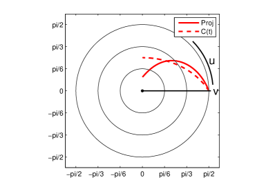
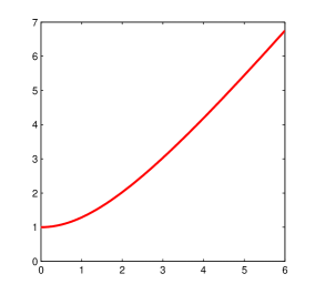
Figure 7: In the figure on the left, the projection $\Pi(c(t))$ (continuous curve) and the trajectory $c(t)$ (dashed curve) are displayed for $t\in[0,100]$. We use $(u,v)$ coordinates (see text). In the figure on the right, $r(t)$ is displayed for $t\in[0,6]$ ($r$ is vertical, time is horizontal).

These figures were produced with the Matlab routine ode45 with AbsTol and RelTol set to $10^{-9}$.

To be absolutely certain that the result is reliable, we recall that we should be able to recover $c(t)=(2,t,t)$ from the solution of equation (19) as follows (see Section 5).

$$c(t)={\boldsymbol{\sigma}}(u(t),v(t))-r(t){\bf n}(t).$$

For the displayed curve we found

$$\max_{t\in[0,100]}\,|{\boldsymbol{\sigma}}(u(t),v(t))-r(t){\bf n}(t)-c(t)|\leq 3\cdot 10^{-7}.$$

• I am indebted to John Milnor for a very useful conversation which led to equation 4, and to Robert Lyons for the numerical results presented in Figure 7.

• received his Ph.D. from Cornell University. He has held visiting positions in the U.S. (Rockefeller University, Stony Brook University, Georgia Tech, Penn State), as well as in Spain, Brazil, Italy, and Greece. He is currently at Portland State University in Oregon, USA, where he is Professor of Mathematics and Affiliate Professor of Physics.

  • Maseeh Department of Mathematics and Statistics, Portland State University, Portland, OR 97201.
    veerman@pdx.edu

References

- 1. Ambrosio, L., Mantegazza, C. (1998). Curvature and distance function from a manifold. J. Geom. Anal. 8(5): 723–748.
- 2. Arnold, V. I. (1992). Ordinary Differential Equations, 3rd ed. Heidelberg: Springer-Verlag.
- 3. Akmal, S. S., Mau Nam, N., Veerman, J. J. P. (2015). On a convex set with nondifferentiable metric projection. Optimization Letters. 9(6): 1039–1052.
- 4. Bernhard, J., Veerman, J. J. P. (2007). The Topology of Surface Mediatrices. Topology and Its Applications 154 (1): 54–68.
- 5. Burago, D., Burago, Y., Ivanov, S. (2001). A Course in Metric Geometry. Graduate Studies in Mathematics 33. Providence, RI: American Mathematical Society.
- 6. Do Carmo, M. P. (1976). Differential Geometry of Curves and Surfaces. Upper Saddle River, NJ: Prentice-Hall.
- 7. Fitzpatrick, S., Phelps, R. R. (1982). Differentiability of the metric projection in Hilbert space. Trans. AMS. 270: 483–501.
- 8. Foote, R. L. (1984). Regularity of the distance function. Proc. AMS. 92(1): 153–155.
- 9. M. Giaquinta, M., Modica, G. (2012). Mathematical Analysis, Foundations and Advanced Techniques for Functions of Several Variables. New York: Springer.
- 10. Ghrist, M. L., Lane, E. E. (2013). Be careful what you assign: Constant speed parametrizations. Math. Mag. 86: 3–14.
- 11. Herreros, P., Ponce, M., Veerman, J. J. P. (2017). Equators have at most countably many singularities with bounded total angle. Annales Academiæ Scientiarum Fennicæ. 42: 837–845.
- 12. Hirsch, M. W., Smale, S., Devaney, R. L. (2013). Differential Equations, Dynamical Systems, and an Introduction to Chaos. Waltham, MA: Academic Press.
- 13. Krantz, S. G., Parks, H. R. (1981). Distance to hypersurfaces, J. Diff. Eq. 40: 116–120.
- 14. Li, Y.-Y., Nirenberg, L. (2005). Regularity of the distance function to the boundary. arxiv.org/abs/math/0510577
- 15. Plaut, C. (2002). Metric spaces of curvature . In: Daverman, R. B., Sher, R. J., Eds. Handbook of Geometric Topology. Amsterdam: North-Holland, pp. 819–898.
- 16. Shapiro, A. (1994). Directionally nondifferentiable metric projection. J. Optim. Theory Appl. 81: 203–204.
- 17. Shapiro, A. (1994). Existence and Differentiability of Metric Projections in Hilbert Spaces. SIAM J. Optim. 4(1): 130-141.
- 18. Veerman, J. J. P., Veerman, Bernhard, J. (2005). Minimally Separating Sets, Mediatrices, and Brillouin Spaces Topology and its Applications 153: 1421-1433.
- 19. Veerman, J. J. P., Peixoto M. M., Rocha, A. C., Sutherland, S., (2000). On Brillouin Zones Communications in Mathematical Physics 212/3: 725-744.
-
J. J. P. VEERMAN