Uncertainty quantification of modified Cahn-Hilliard equation for image inpainting

Yin Xian Department of Mathematics, Hong Kong University of Science and Technology, Clear Water Bay, Hong Kong
(June 2019)

Abstract

In this paper, we review modified Cahn-Hilliard equation for image inpainting and explore the effect when the initial condition is uncertain. We study the statistical properties of the solution when the noise is present. The generalized polynomial chaos and the perturbation expansion are used to analyze the equation. Experimental results are attached for comparison of solution behavior.

1 Introduction

1.1 PDE based image inpainting

Given an observed image g𝑔g, which is corrupted, we want to have the original image u𝑒u.

T​u=g𝑇𝑒𝑔\displaystyle Tu=g

where T𝑇T models the process through which the image u𝑒u went through observation. Let Ξ©βˆˆβ„2Ξ©superscriptℝ2\Omega\in\mathbb{R}^{2} be a given domain, B1subscript𝐡1B_{1} be banach spaces over ΩΩ\Omega and g∈B1𝑔subscript𝐡1g\in B_{1} be the given image. A general variational approach in image processing can be written as:

J​(u)=R​(u)+12​λ​‖T​uβˆ’gβ€–B12𝐽𝑒𝑅𝑒12πœ†subscriptsuperscriptnorm𝑇𝑒𝑔2subscript𝐡1\displaystyle J(u)=R(u)+\frac{1}{2\lambda}||Tu-g||^{2}_{B_{1}} (1)

where Ξ»πœ†\lambda is the tuning parameter of the problem and Tβˆˆβ„’β€‹(B1)𝑇ℒsubscript𝐡1T\in\mathcal{L}(B_{1}) is a bounded linear operator. R𝑅R denotes the regularizing term which smoothes the image u𝑒u and represents some kind of a priori information about the minimizer u𝑒u. β€–T​uβˆ’gβ€–B12superscriptsubscriptnorm𝑇𝑒𝑔subscript𝐡12||Tu-g||_{B_{1}}^{2} is called fidelity term of the approach which forces the minimizer u𝑒u to stay close to the given image g𝑔g.

For B1=L2​(Ξ©)subscript𝐡1superscript𝐿2Ξ©B_{1}=L^{2}(\Omega) we also have the corresponding Euler-Lagrange equation:

βˆ’Ξ»β€‹βˆ‡R​(u)+Tβˆ—β€‹(gβˆ’T​u)=0,inΒ β€‹Ξ©πœ†βˆ‡π‘…π‘’superscript𝑇𝑔𝑇𝑒0inΒ Ξ©\displaystyle-\lambda\nabla R(u)+T^{*}(g-Tu)=0,\leavevmode\nobreak\ \leavevmode\nobreak\ \leavevmode\nobreak\ \leavevmode\nobreak\ \text{in\leavevmode\nobreak\ }\Omega (2)

the corresponding steepest descent equation for u𝑒u is the given image

ut=βˆ’Ξ»β€‹βˆ‡R​(u)+Tβˆ—β€‹(gβˆ’T​u),in ​Ωsubscriptπ‘’π‘‘πœ†βˆ‡π‘…π‘’superscript𝑇𝑔𝑇𝑒inΒ Ξ©\displaystyle u_{t}=-\lambda\nabla R(u)+T^{*}(g-Tu),\leavevmode\nobreak\ \leavevmode\nobreak\ \leavevmode\nobreak\ \text{in\leavevmode\nobreak\ }\Omega

For Cahn-Hilliard equation and TV-Hβˆ’1superscript𝐻1H^{-1} inpainting, the image processing approach is directly given by an evolutionary PDE. A regularizing term which can delete noise and preserve important image features like edges is the total variation.

J​(u)=R​(u)+12​λ​‖χΩ\D​(uβˆ’g)β€–B12𝐽𝑒𝑅𝑒12πœ†superscriptsubscriptnormsubscriptπœ’\Ω𝐷𝑒𝑔subscript𝐡12\displaystyle J(u)=R(u)+\frac{1}{2\lambda}||\chi_{\Omega\backslash D}(u-g)||_{B_{1}}^{2} (3)

where

χΩ\D​(x)={1,Ξ©\D0,∈D\displaystyle\chi_{\Omega\backslash D}(x)=\left\{\begin{array}[]{ll}1,\leavevmode\nobreak\ \leavevmode\nobreak\ \Omega\backslash D\\ 0,\leavevmode\nobreak\ \leavevmode\nobreak\ \in D\end{array}\right.

R​(u)𝑅𝑒R(u) fills in the image content into the missing domain D𝐷D, by diffusion and transport. The fidelity term only has impact on the minimizer u𝑒u outside of the inpainting domain due to the characteristic function χΩ\Dsubscriptπœ’\Ω𝐷\chi_{\Omega\backslash D}. For R​(u)𝑅𝑒R(u) we have,

  • β€’

    R​(u)=∫Ω|βˆ‡u|2​𝑑x𝑅𝑒subscriptΞ©superscriptβˆ‡π‘’2differential-dπ‘₯R(u)=\int_{\Omega}|\nabla u|^{2}dx, harmonic inpainting.

  • β€’

    R​(u)=∫Ω|βˆ‡u|​𝑑x𝑅𝑒subscriptΞ©βˆ‡π‘’differential-dπ‘₯R(u)=\int_{\Omega}|\nabla u|dx, TV-inpainting, (Chan and Shen 2001).

  • β€’

    R(u)=∫Ω(1+βˆ‡β‹…(βˆ‡u|βˆ‡u|)))|βˆ‡u|dxR(u)=\int_{\Omega}(1+\nabla\cdot(\frac{\nabla u}{|\nabla u|})))|\nabla u|dx, Euler’s elastica inpainting

  • β€’

    inpainting for binary images with the Cahn-Hilliard equation, (Bertozzi, Esedoglu and Gillette 06)

  • β€’

    TV-Hβˆ’1superscript𝐻1H^{-1} inpainting, (Burger, He).

For TV inpainting, it propagate sharp edges into the damaged domain

minuβ€‹βˆ«Ξ©|βˆ‡u|​𝑑x⟺minΞ“Ξ»β€‹βˆ«βˆ’βˆžβˆžlength​(Γλ)β€‹π‘‘Ξ»βŸΊsubscript𝑒subscriptΞ©βˆ‡π‘’differential-dπ‘₯subscriptsubscriptΞ“πœ†superscriptsubscriptlengthsubscriptΞ“πœ†differential-dπœ†\displaystyle\min\limits_{u}\int_{\Omega}|\nabla u|dx\Longleftrightarrow\min\limits_{\Gamma_{\lambda}}\int_{-\infty}^{\infty}\text{length}(\Gamma_{\lambda})d\lambda (4)

where Γλ={x∈Ω:u​(x)=Ξ»}subscriptΞ“πœ†conditional-setπ‘₯Ω𝑒π‘₯πœ†\Gamma_{\lambda}=\{x\in\Omega:u(x)=\lambda\}. It penalizes length of edges, cannot connect contours across very large distances, it can result in corners of the level lines across the inpainting domain.

For higher order approaches, often they do not posses a maximum principle or comparison principle. For the proof of well-posedness of higher order inpainting models variational methods are often not applicable, and it need stable and fast numerical solvers.

minuβ€‹βˆ«Ξ©(a+bβ€‹βˆ‡β‹…(βˆ‡u|βˆ‡u|))​|βˆ‡u|​𝑑x⟺minΞ“Ξ»β€‹βˆ«βˆ’βˆžβˆž(a​length​(Γλ)+b​curvature​(Γλ))β€‹π‘‘Ξ»βŸΊsubscript𝑒subscriptΞ©π‘Žβ‹…π‘βˆ‡βˆ‡π‘’βˆ‡π‘’βˆ‡π‘’differential-dπ‘₯subscriptsubscriptΞ“πœ†superscriptsubscriptπ‘ŽlengthsubscriptΞ“πœ†π‘curvaturesubscriptΞ“πœ†differential-dπœ†\displaystyle\min\limits_{u}\int_{\Omega}\left(a+b\nabla\cdot\left(\frac{\nabla u}{|\nabla u|}\right)\right)|\nabla u|dx\Longleftrightarrow\min\limits_{\Gamma_{\lambda}}\int_{-\infty}^{\infty}(a\leavevmode\nobreak\ \text{length}(\Gamma_{\lambda})+b\leavevmode\nobreak\ \text{curvature}(\Gamma_{\lambda}))d\lambda

1.2 Modified Cahn-Hilliard equation

(Analytical challenges) Results for stationary solution are difficult because of the missing energy for the equation.

ut=Δ​(βˆ’Ξ΅β€‹Ξ”β€‹u+1Ρ​W′​(u))+λ​χΩ\D​(fβˆ’u)subscriptπ‘’π‘‘Ξ”πœ€Ξ”π‘’1πœ€superscriptπ‘Šβ€²π‘’πœ†subscriptπœ’\Ω𝐷𝑓𝑒\displaystyle u_{t}=\Delta(-\varepsilon\Delta u+\frac{1}{\varepsilon}W^{\prime}(u))+\lambda\chi_{\Omega\backslash D}(f-u) (5)

W​(u)π‘Šπ‘’W(u) is a double well potential. The two wells of Wπ‘ŠW correspond to values of u𝑒u that are taken by most of the grey scale values. Ξ»>>0much-greater-thanπœ†0\lambda>>0. By choosing a potential with wells at the values 0 (black) and 1 (white), therefore provides a simple model for the inpainting of binary images. The parameter Ξ΅>0πœ€0\varepsilon>0 determines the steepness of the transition between 0 and 1.

The Cahn-Hilliard equation is a relatively simple fourth order PDE used for this task rather than more complex models involving curvature terms such as Euler-Elastica inpainting. It has many of the desirable properties of curvature-based inpainting models such as the smooth continuation of level lines into the missing domainΒ [6].

The gradient flow in Hβˆ’1superscript𝐻1H^{-1} of the energy is given by

J1​(u)=∫ΩΡ2​|βˆ‡u|2+1Ρ​W​(u)​d​x.superscript𝐽1𝑒subscriptΞ©πœ€2superscriptβˆ‡π‘’21πœ€π‘Šπ‘’π‘‘π‘₯\displaystyle J^{1}(u)=\int_{\Omega}\frac{\varepsilon}{2}|\nabla u|^{2}+\frac{1}{\varepsilon}W(u)dx.

The gradient flow in L2superscript𝐿2L^{2} of the energy is given by

J2​(u)=Ξ»2β€‹βˆ«Ξ©Ο‡Ξ©\D​(fβˆ’u)2​𝑑xsuperscript𝐽2π‘’πœ†2subscriptΞ©subscriptπœ’\Ω𝐷superscript𝑓𝑒2differential-dπ‘₯\displaystyle J^{2}(u)=\frac{\lambda}{2}\int_{\Omega}\chi_{\Omega\backslash D}(f-u)^{2}dx

The global existence for the evolution equation is given by Bertozzi, Esedoglu and Gillette 06, the authors proved that in the limit Ξ»β†’βˆžβ†’πœ†\lambda\to\infty, a stationary solution solves

βˆ‡(Ξ΅β€‹βˆ‡uβˆ’1Ρ​W′​(u))βˆ‡πœ€βˆ‡π‘’1πœ€superscriptπ‘Šβ€²π‘’\displaystyle\nabla(\varepsilon\nabla u-\frac{1}{\varepsilon}W^{\prime}(u)) =0,Β inD,absent0Β in𝐷\displaystyle=0,\leavevmode\nobreak\ \leavevmode\nobreak\ \text{ in}\leavevmode\nobreak\ \leavevmode\nobreak\ D,
u𝑒\displaystyle u =fΒ onβˆ‚D,absent𝑓 on𝐷\displaystyle=f\leavevmode\nobreak\ \leavevmode\nobreak\ \text{ on}\leavevmode\nobreak\ \leavevmode\nobreak\ \partial D,
βˆ‡uβˆ‡π‘’\displaystyle\nabla u =βˆ‡fΒ onβˆ‚D,absentβˆ‡π‘“Β on𝐷\displaystyle=\nabla f\leavevmode\nobreak\ \leavevmode\nobreak\ \text{ on}\leavevmode\nobreak\ \leavevmode\nobreak\ \partial D,

for f𝑓f regular enough (f∈C2𝑓superscript𝐢2f\in C^{2}). The existence of a stationary solution to the modified Cahn-Hilliard equation is proved by using the idea of fixed point equation. This claim that fourth-order methods are superior to second order methods with respect to a smooth continuation of the image contents into the missing domain. Combined with other inpainting strategies, it can constitute a powerful method for inpainting of the structural part of an imageΒ [6].

The sequence of Cahn-Hilliard functionals:

∫Ω(Ξ΅2​|βˆ‡u|2+1Ρ​W​(u))​𝑑xsubscriptΞ©πœ€2superscriptβˆ‡π‘’21πœ€π‘Šπ‘’differential-dπ‘₯\displaystyle\int_{\Omega}(\frac{\varepsilon}{2}|\nabla u|^{2}+\frac{1}{\varepsilon}W(u))dx

ΓΓ\Gamma-convergence in the topology L1​(Ξ©)superscript𝐿1Ξ©L^{1}(\Omega) to

T​V​(u)={C0​|D​u|​(Ξ©),ifΒ |u​(x)|=1Β inΒ Ξ©+∞,o​t​h​e​r​w​i​s​e𝑇𝑉𝑒casessubscript𝐢0𝐷𝑒ΩifΒ |u(x)|=1Β inΒ Ξ©missing-subexpressionπ‘œπ‘‘β„Žπ‘’π‘Ÿπ‘€π‘–π‘ π‘’missing-subexpression\displaystyle TV(u)=\left\{\begin{array}[]{ll}C_{0}|Du|(\Omega),\leavevmode\nobreak\ \leavevmode\nobreak\ \text{if $|u(x)|=1$ in $\Omega$}\\ +\infty,\leavevmode\nobreak\ \leavevmode\nobreak\ otherwise\end{array}\right. (8)

as Ξ΅β†’0β†’πœ€0\varepsilon\to 0, where C0=2β€‹βˆ«βˆ’11F​(s)​𝑑ssubscript𝐢02superscriptsubscript11𝐹𝑠differential-d𝑠C_{0}=2\int_{-1}^{1}\sqrt{F(s)}ds. Motivated by the ΓΓ\Gamma-convergence, the TV-Hβˆ’1superscript𝐻1H^{-1} method is proposed. The inpainted image u𝑒u of f∈L2​(Ξ©)𝑓superscript𝐿2Ξ©f\in L^{2}(\Omega) shall evolve via

ut=Δ​p+λ​χΩ\D​(fβˆ’u),pβˆˆβˆ‚TV​(u)formulae-sequencesubscriptπ‘’π‘‘Ξ”π‘πœ†subscriptπœ’\Ω𝐷𝑓𝑒𝑝TV𝑒\displaystyle u_{t}=\Delta p+\lambda\chi_{\Omega\backslash D}(f-u),\leavevmode\nobreak\ \leavevmode\nobreak\ \leavevmode\nobreak\ p\in\partial\text{TV}(u)

where βˆ‚\partialTV(u) denotes the subdifferential of

T​V​(u)={|D​u|​(Ξ©),ifΒ |u​(x)|≀1Β inΒ Ξ©+∞,o​t​h​e​r​w​i​s​e𝑇𝑉𝑒cases𝐷𝑒ΩifΒ |u(x)|≀1Β inΒ Ξ©missing-subexpressionπ‘œπ‘‘β„Žπ‘’π‘Ÿπ‘€π‘–π‘ π‘’missing-subexpression\displaystyle TV(u)=\left\{\begin{array}[]{ll}|Du|(\Omega),\leavevmode\nobreak\ \leavevmode\nobreak\ \text{if $|u(x)|\leq 1$ in $\Omega$}\\ +\infty,\leavevmode\nobreak\ \leavevmode\nobreak\ otherwise\end{array}\right. (11)

By using the existence of stationary solution in the Cahn-Hilliard case, it can be proved that

Δ​p+λ​χΩ\D​(fβˆ’u)=0,pβˆˆβˆ‚T​V​(u)formulae-sequenceΞ”π‘πœ†subscriptπœ’\Ω𝐷𝑓𝑒0𝑝𝑇𝑉𝑒\displaystyle\Delta p+\lambda\chi_{\Omega\backslash D}(f-u)=0,\leavevmode\nobreak\ \leavevmode\nobreak\ \leavevmode\nobreak\ p\in\partial TV(u) (12)

admits a solution u∈B​V​(Ξ©)𝑒𝐡𝑉Ωu\in BV(\Omega)

2 Cahn-Hilliard equation on image inpainting

Bertozzi et al. introduced the fourth order Cahn-Hilliard inpainting approach for binary, i.e., black and white, imagesΒ [3]. This model is based on scalar smooth Cahn-Hilliard equation. The binary Cahn-Hilliard inpainting model has been generalized to gray value imagesΒ [4]. This model is based on vector valued Cahn-Hilliard equation. (RGB for image of three channels, which corresponds three different chemical in fluid dynamics)

2.1 Binary images

Let f(x,y) be a given image in a domain ΩΩ\Omega, and suppose that DβŠ‚Ξ©π·Ξ©D\subset\Omega is the inpainting domain. Let u​(x,y,t)𝑒π‘₯𝑦𝑑u(x,y,t) evolve in time to become a fully inpainted version of f​(x,y)𝑓π‘₯𝑦f(x,y) under the equation:

ut=βˆ’Ξ”β€‹(Ρ​Δ​uβˆ’1Ρ​W′​(u))+λ​(x,y)​(fβˆ’u)subscriptπ‘’π‘‘Ξ”πœ€Ξ”π‘’1πœ€superscriptπ‘Šβ€²π‘’πœ†π‘₯𝑦𝑓𝑒\displaystyle u_{t}=-\Delta(\varepsilon\Delta u-\frac{1}{\varepsilon}W^{\prime}(u))+\lambda(x,y)(f-u) (13)

where

λ​(x,y)={0,if ​(x,y)∈DΞ»0,if ​(x,y)∈Ω\Dπœ†π‘₯𝑦cases0ifΒ π‘₯𝑦𝐷missing-subexpressionsubscriptπœ†0ifΒ π‘₯𝑦\Ω𝐷missing-subexpression\displaystyle\lambda(x,y)=\left\{\begin{array}[]{ll}0,\leavevmode\nobreak\ \leavevmode\nobreak\ \leavevmode\nobreak\ \text{if }(x,y)\in D\\ \lambda_{0},\leavevmode\nobreak\ \leavevmode\nobreak\ \leavevmode\nobreak\ \text{if }(x,y)\in\Omega\backslash D\end{array}\right.

The function W​(u)π‘Šπ‘’W(u) is a nonlinear potential with wells corresponding to values of u𝑒u that are taken on by most of the grayscale values. In the binary case, Wπ‘ŠW should have wells at the values u=0𝑒0u=0 and u=1𝑒1u=1. We use the function W​(u)=u2​(uβˆ’1)2π‘Šπ‘’superscript𝑒2superscript𝑒12W(u)=u^{2}(u-1)^{2}. We use convexity splitting.

The modified Cahn-Hilliard equation is not strictly a gradient flow. The original Cahn-Hilliard equation is indeed a gradient flow using an Hβˆ’1superscript𝐻1H^{-1} norm for the energy.

E1=∫ΩΡ2​|βˆ‡u|2+1Ρ​W​(u)​d​xsubscript𝐸1subscriptΞ©πœ€2superscriptβˆ‡π‘’21πœ€π‘Šπ‘’π‘‘π‘₯\displaystyle E_{1}=\int_{\Omega}\frac{\varepsilon}{2}|\nabla u|^{2}+\frac{1}{\varepsilon}W(u)dx

The fidelity term of eq. 13 can be derived from a gradient flow under an L2superscript𝐿2L^{2} norm for the energy.

E2=Ξ»0β€‹βˆ«Ξ©\D(fβˆ’u)2​𝑑xsubscript𝐸2subscriptπœ†0subscript\Ω𝐷superscript𝑓𝑒2differential-dπ‘₯\displaystyle E_{2}=\lambda_{0}\int_{\Omega\backslash D}(f-u)^{2}dx (14)

We can split E1subscript𝐸1E_{1} as

E1=E11βˆ’E12subscript𝐸1subscript𝐸11subscript𝐸12\displaystyle E_{1}=E_{11}-E_{12} (15)

where

E11subscript𝐸11\displaystyle E_{11} =∫ΩΡ2​|βˆ‡u|2+C12​|u|2​d​xabsentsubscriptΞ©πœ€2superscriptβˆ‡π‘’2subscript𝐢12superscript𝑒2𝑑π‘₯\displaystyle=\int_{\Omega}\frac{\varepsilon}{2}|\nabla u|^{2}+\frac{C_{1}}{2}|u|^{2}dx
E12subscript𝐸12\displaystyle E_{12} =βˆ«Ξ©βˆ’1Ρ​W​(u)+C12​|u|2​d​xabsentsubscriptΞ©1πœ€π‘Šπ‘’subscript𝐢12superscript𝑒2𝑑π‘₯\displaystyle=\int_{\Omega}-\frac{1}{\varepsilon}W(u)+\frac{C_{1}}{2}|u|^{2}dx

A possible splitting for E2subscript𝐸2E_{2} is

E2=E21βˆ’E22subscript𝐸2subscript𝐸21subscript𝐸22\displaystyle E_{2}=E_{21}-E_{22}

where

E21subscript𝐸21\displaystyle E_{21} =∫Ω\DC22​|u|2​𝑑xabsentsubscript\Ω𝐷subscript𝐢22superscript𝑒2differential-dπ‘₯\displaystyle=\int_{\Omega\backslash D}\frac{C_{2}}{2}|u|^{2}dx
E22subscript𝐸22\displaystyle E_{22} =∫Ω\Dβˆ’Ξ»0​(fβˆ’u)2+C22​|u|2​d​xabsentsubscript\Ω𝐷subscriptπœ†0superscript𝑓𝑒2subscript𝐢22superscript𝑒2𝑑π‘₯\displaystyle=\int_{\Omega\backslash D}-\lambda_{0}(f-u)^{2}+\frac{C_{2}}{2}|u|^{2}dx

For this splittings, the resulting time-stepping scheme is:

un+1βˆ’unΔ​t=βˆ’βˆ‡Hβˆ’1(E11n+1βˆ’E12n)βˆ’βˆ‡L2(E21n+1βˆ’E22n)superscript𝑒𝑛1superscript𝑒𝑛Δ𝑑subscriptβˆ‡superscript𝐻1superscriptsubscript𝐸11𝑛1superscriptsubscript𝐸12𝑛subscriptβˆ‡superscript𝐿2superscriptsubscript𝐸21𝑛1superscriptsubscript𝐸22𝑛\displaystyle\frac{u^{n+1}-u^{n}}{\Delta t}=-\nabla_{H^{-1}}(E_{11}^{n+1}-E_{12}^{n})-\nabla_{L^{2}}(E_{21}^{n+1}-E_{22}^{n})

where βˆ‡Hβˆ’1subscriptβˆ‡superscript𝐻1\nabla_{H^{-1}} and βˆ‡L2subscriptβˆ‡superscript𝐿2\nabla_{L^{2}} represent gradient descent with respect to the Hβˆ’1superscript𝐻1H^{-1} inner product, and L2superscript𝐿2L^{2} inner product, respectively. This translates to a numerical scheme of the form

un+1​(x,y)βˆ’un​(x,y)βˆ‚t+Ρ​Δ2​un+1​(x,y)βˆ’C1​Δ​un+1​(x,y)+C2​un+1​(x,y)superscript𝑒𝑛1π‘₯𝑦superscript𝑒𝑛π‘₯π‘¦π‘‘πœ€superscriptΞ”2superscript𝑒𝑛1π‘₯𝑦subscript𝐢1Ξ”superscript𝑒𝑛1π‘₯𝑦subscript𝐢2superscript𝑒𝑛1π‘₯𝑦\displaystyle\frac{u^{n+1}(x,y)-u^{n}(x,y)}{\partial t}+\varepsilon\Delta^{2}u^{n+1}(x,y)-C_{1}\Delta u^{n+1}(x,y)+C_{2}u^{n+1}(x,y)
=\displaystyle= Δ​(1Ρ​W′​(un​(x,y)))+λ​(x,y)​(f​(x,y)βˆ’un​(x,y))βˆ’C1​Δ​un​(x,y)+C2​un​(x,y)Ξ”1πœ€superscriptπ‘Šβ€²superscript𝑒𝑛π‘₯π‘¦πœ†π‘₯𝑦𝑓π‘₯𝑦superscript𝑒𝑛π‘₯𝑦subscript𝐢1Ξ”superscript𝑒𝑛π‘₯𝑦subscript𝐢2superscript𝑒𝑛π‘₯𝑦\displaystyle\Delta(\frac{1}{\varepsilon}W^{\prime}(u^{n}(x,y)))+\lambda(x,y)(f(x,y)-u^{n}(x,y))-C_{1}\Delta u^{n}(x,y)+C_{2}u^{n}(x,y)

The constant C1subscript𝐢1C_{1} and C2subscript𝐢2C_{2} are positive, and need to be chosen large enough so that the energies E11,E12,E21subscript𝐸11subscript𝐸12subscript𝐸21E_{11},E_{12},E_{21} and E22subscript𝐸22E_{22} are convex. C1subscript𝐢1C_{1} should be comparable to 1Ξ΅1πœ€\frac{1}{\varepsilon}, while C2subscript𝐢2C_{2} should be comparable to Ξ»0subscriptπœ†0\lambda_{0}. We can use the spectral method and finite element method to solve this numerical PDE, to obtain an approximated solution of u𝑒u.

2.2 Color images

Let f𝑓f be the given gray value image, which is defined on the image domain Ξ©βˆˆβ„lΞ©superscriptℝ𝑙\Omega\in\mathbb{R}^{l}, with l∈{2,3}𝑙23l\in\{2,3\}. Let Yπ‘ŒY be the number of gray values which form the image. These Yπ‘ŒY gray values are collected in the vector π•˜=[g1,g2,β‹―,gY]Tβˆˆβ„Yπ•˜superscriptsubscript𝑔1subscript𝑔2β‹―subscriptπ‘”π‘Œπ‘‡superscriptβ„π‘Œ\mathbb{g}=[g_{1},g_{2},\cdots,g_{Y}]^{T}\in\mathbb{R}^{Y}, and 2≀Y≀2562π‘Œ2562\leq Y\leq 256. The target is to reconstruct the image f𝑓f in the inpainting region D𝐷D. Denote the reconstructed image by frsubscriptπ‘“π‘Ÿf_{r}. Let T>0𝑇0T>0 be a fixed time. Introducing a vector-valued phase variables 𝕦=[u1,β‹―,uY]T:Ω×(0,T)→ℝY:𝕦superscriptsubscript𝑒1β‹―subscriptπ‘’π‘Œπ‘‡β†’Ξ©0𝑇superscriptβ„π‘Œ\mathbb{u}=[u_{1},\cdots,u_{Y}]^{T}:\Omega\times(0,T)\rightarrow\mathbb{R}^{Y}. uisubscript𝑒𝑖u_{i} describes the concentration of gray value gisubscript𝑔𝑖g_{i} for i=1,β‹―,Y𝑖1β‹―π‘Œi=1,\cdots,Y. If ui​(𝕩,t)β‰ˆ1subscript𝑒𝑖𝕩𝑑1u_{i}(\mathbb{x},t)\approx 1, then only gray value gisubscript𝑔𝑖g_{i} is present at point 𝕩𝕩\mathbb{x} at time t𝑑t. ui​(𝕩,t)β‰ˆ0subscript𝑒𝑖𝕩𝑑0u_{i}(\mathbb{x},t)\approx 0 means gray value gisubscript𝑔𝑖g_{i} is absent at point 𝕩𝕩\mathbb{x} at time t𝑑t. Values of uisubscript𝑒𝑖u_{i} between 00 and 111 represent mixed regions. We initialize uisubscript𝑒𝑖u_{i} with ui​(𝕩,0)=fi​(𝕩)subscript𝑒𝑖𝕩0subscript𝑓𝑖𝕩u_{i}(\mathbb{x},0)=f_{i}(\mathbb{x}). The evolution of the reconstructed image frsubscriptπ‘“π‘Ÿf_{r} is obtained from the components uisubscript𝑒𝑖u_{i} via,

fr=βˆ‘i=1Ygi​uisubscriptπ‘“π‘Ÿsuperscriptsubscript𝑖1π‘Œsubscript𝑔𝑖subscript𝑒𝑖\displaystyle f_{r}=\sum\limits_{i=1}^{Y}g_{i}u_{i}

We have βˆ‘i=1Yui=1superscriptsubscript𝑖1π‘Œsubscript𝑒𝑖1\sum\limits_{i=1}^{Y}u_{i}=1. The final reconstructed image frsubscriptπ‘“π‘Ÿf_{r} of f𝑓f is fr​(𝕩,T)subscriptπ‘“π‘Ÿπ•©π‘‡f_{r}(\mathbb{x},T).

The Cahn-Hilliard inpainting model is based on the Ginzburg-Landau energy E1subscript𝐸1E_{1}.

E1​(𝕦)=∫ΩΡ2β€‹βˆ‘i=1Y|βˆ‡ui|2+1Ρ​W​(𝕦)​d​𝕩subscript𝐸1𝕦subscriptΞ©πœ€2superscriptsubscript𝑖1π‘Œsuperscriptβˆ‡subscript𝑒𝑖21πœ€π‘Šπ•¦π‘‘π•©\displaystyle E_{1}(\mathbb{u})=\int_{\Omega}\frac{\varepsilon}{2}\sum\limits_{i=1}^{Y}|\nabla u_{i}|^{2}+\frac{1}{\varepsilon}W(\mathbb{u})d\mathbb{x}

According to [4], the smooth gray value Cahn-Hilliard equation is

{βˆ‚tui=Δ​wi+λ​(fiβˆ’ui)wi=βˆ’Ξ΅β€‹Ξ”β€‹ui+1Ρ​W′​(ui)βˆ’1Ρ​Nβ€‹βˆ‘j=1NW′​(uj)βˆ‡uiβ‹…π•Ÿ=βˆ‡wiβ‹…π•Ÿ=0onΒ β€‹βˆ‚Ξ©casesmissing-subexpressionsubscript𝑑subscript𝑒𝑖Δsubscriptπ‘€π‘–πœ†subscript𝑓𝑖subscript𝑒𝑖missing-subexpressionmissing-subexpressionsubscriptπ‘€π‘–πœ€Ξ”subscript𝑒𝑖1πœ€superscriptπ‘Šβ€²subscript𝑒𝑖1πœ€π‘superscriptsubscript𝑗1𝑁superscriptπ‘Šβ€²subscript𝑒𝑗missing-subexpressionmissing-subexpressionformulae-sequenceβˆ‡β‹…subscriptπ‘’π‘–π•Ÿβˆ‡β‹…subscriptπ‘€π‘–π•Ÿ0onΒ Ξ©missing-subexpression\displaystyle\left\{\begin{array}[]{lll}&\partial_{t}u_{i}=\Delta w_{i}+\lambda(f_{i}-u_{i})\\ &w_{i}=-\varepsilon\Delta u_{i}+\frac{1}{\varepsilon}W^{\prime}(u_{i})-\frac{1}{\varepsilon N}\sum\limits_{j=1}^{N}W^{\prime}(u_{j})\\ &\nabla u_{i}\cdot\mathbb{n}=\nabla w_{i}\cdot\mathbb{n}=0\leavevmode\nobreak\ \leavevmode\nobreak\ \leavevmode\nobreak\ \text{on\leavevmode\nobreak\ \leavevmode\nobreak\ }\partial\Omega\end{array}\right.

where W​(u)=u2​(uβˆ’1)2π‘Šπ‘’superscript𝑒2superscript𝑒12W(u)=u^{2}(u-1)^{2}.

3 Randomness, Stochastic Galerkin method

When there is noise in the image, the initial condition of the Cahn-Hilliard equation will have uncertainty. We therefore introduce random variable Z𝑍Z to the modified Cahn-Hilliard equation.

3.1 Polynomial approximation

Let β„™nsubscriptℙ𝑛\mathbb{P}_{n} be the linear space of polynomials of degree at most n𝑛n:

β„™n=span​{xk:k=0,1,β‹―,n}.subscriptℙ𝑛spanconditional-setsuperscriptπ‘₯π‘˜π‘˜01⋯𝑛\displaystyle\mathbb{P}_{n}=\text{span}\{x^{k}:k=0,1,\cdots,n\}.

Weierstrass approximation theory: Let I𝐼I be a bounded interval and let f∈C0​(IΒ―)𝑓superscript𝐢0¯𝐼f\in C^{0}(\bar{I}). Then, for any Ο΅>0italic-Ο΅0\epsilon>0, we can find nβˆˆβ„•π‘›β„•n\in\mathbb{N} and pβˆˆβ„™n𝑝subscriptℙ𝑛p\in\mathbb{P}_{n} such that

|f​(x)βˆ’p​(x)|<Ο΅,βˆ€x∈IΒ―formulae-sequence𝑓π‘₯𝑝π‘₯italic-Ο΅for-allπ‘₯¯𝐼\displaystyle|f(x)-p(x)|<\epsilon,\leavevmode\nobreak\ \leavevmode\nobreak\ \leavevmode\nobreak\ \leavevmode\nobreak\ \leavevmode\nobreak\ \leavevmode\nobreak\ \forall x\in\bar{I}

In other words, we would like to study the existence of Ο•n​(f)βˆˆβ„™nsubscriptitalic-ϕ𝑛𝑓subscriptℙ𝑛\phi_{n}(f)\in\mathbb{P}_{n} such that

β€–fβˆ’Ο•n​(f)β€–βˆž=infΟˆβˆˆβ„™nβ€–fβˆ’Οˆβ€–βˆžsubscriptnorm𝑓subscriptitalic-ϕ𝑛𝑓subscriptinfimumπœ“subscriptℙ𝑛subscriptnormπ‘“πœ“\displaystyle||f-\phi_{n}(f)||_{\infty}=\inf_{\begin{subarray}{c}\psi\in\mathbb{P}_{n}\end{subarray}}||f-\psi||_{\infty} (16)

The n𝑛nth-degree polynomial Ο•n​(f)subscriptitalic-ϕ𝑛𝑓\phi_{n}(f) is called the polynomial of best uniform approximation of f𝑓f in I¯¯𝐼\bar{I}.

Another approximation problem can be formulated in terms of norms other than the infinity norm used in eq.Β (16). For a positive weight function w​(x)𝑀π‘₯w(x), x∈Iπ‘₯𝐼x\in I, the weighted L2superscript𝐿2L^{2} space by:

Lw2​(I)={v:I→ℝ|∫Iv2​(x)​w​(x)​𝑑x<∞}superscriptsubscript𝐿𝑀2𝐼conditional-set𝑣→𝐼conditionalℝsubscript𝐼superscript𝑣2π‘₯𝑀π‘₯differential-dπ‘₯\displaystyle L_{w}^{2}(I)=\left\{v:I\rightarrow\mathbb{R}|\int_{I}v^{2}(x)w(x)dx<\infty\right\}

with the inner product

(u,v)Lw2​(I)=∫Iu​(x)​v​(x)​w​(x)​𝑑x,βˆ€u,v∈Lw2​(I),formulae-sequencesubscript𝑒𝑣superscriptsubscript𝐿𝑀2𝐼subscript𝐼𝑒π‘₯𝑣π‘₯𝑀π‘₯differential-dπ‘₯for-all𝑒𝑣superscriptsubscript𝐿𝑀2𝐼\displaystyle(u,v)_{L_{w}^{2}(I)}=\int_{I}u(x)v(x)w(x)dx,\leavevmode\nobreak\ \leavevmode\nobreak\ \leavevmode\nobreak\ \leavevmode\nobreak\ \leavevmode\nobreak\ \leavevmode\nobreak\ \forall u,v\in L_{w}^{2}(I),

and the norm

β€–uβ€–Lw2​(I)=(∫Iu2​(x)​w​(x)​𝑑x)1/2.subscriptnorm𝑒superscriptsubscript𝐿𝑀2𝐼superscriptsubscript𝐼superscript𝑒2π‘₯𝑀π‘₯differential-dπ‘₯12\displaystyle||u||_{L_{w}^{2}(I)}=\left(\int_{I}u^{2}(x)w(x)dx\right)^{1/2}.

3.1.1 Orthogonal Projection

Let N𝑁N be a fixed nonnegative integer and let {Ο•k​(x)}k=0NβŠ‚β„™Nsuperscriptsubscriptsubscriptitalic-Ο•π‘˜π‘₯π‘˜0𝑁subscriptℙ𝑁\{\phi_{k}(x)\}_{k=0}^{N}\subset\mathbb{P}_{N} be orthogonal polynomials of degree at most N𝑁N with respect to the positive weight w​(x)𝑀π‘₯w(x).

(Ο•m​(x),Ο•n​(x))Lw2​(I)=β€–Ο•mβ€–Lw2​(I)2​δm,n, 0≀m,n≀N.formulae-sequencesubscriptsubscriptitalic-Ο•π‘šπ‘₯subscriptitalic-ϕ𝑛π‘₯superscriptsubscript𝐿𝑀2𝐼subscriptsuperscriptnormsubscriptitalic-Ο•π‘š2superscriptsubscript𝐿𝑀2𝐼subscriptπ›Ώπ‘šπ‘›formulae-sequence 0π‘šπ‘›π‘\displaystyle(\phi_{m}(x),\phi_{n}(x))_{L_{w}^{2}(I)}=||\phi_{m}||^{2}_{L_{w}^{2}(I)}\delta_{m,n},\leavevmode\nobreak\ \leavevmode\nobreak\ \leavevmode\nobreak\ \leavevmode\nobreak\ \leavevmode\nobreak\ 0\leq m,n\leq N.

The projection operator PN:Lw2​(I)β†’β„™N:subscript𝑃𝑁→superscriptsubscript𝐿𝑀2𝐼subscriptℙ𝑁P_{N}:L_{w}^{2}(I)\rightarrow\mathbb{P}_{N}, for any function f∈Lw2​(I)𝑓superscriptsubscript𝐿𝑀2𝐼f\in L_{w}^{2}(I)

PN​f=βˆ‘k=0Nf^k​ϕk​(x)subscript𝑃𝑁𝑓superscriptsubscriptπ‘˜0𝑁subscript^π‘“π‘˜subscriptitalic-Ο•π‘˜π‘₯\displaystyle P_{N}f=\sum\limits_{k=0}^{N}\hat{f}_{k}\phi_{k}(x)

where

f^k=1β€–Ο•kβ€–Lw22​(f,Ο•k)Lw2, 0≀k≀Nformulae-sequencesubscript^π‘“π‘˜1subscriptsuperscriptnormsubscriptitalic-Ο•π‘˜2superscriptsubscript𝐿𝑀2subscript𝑓subscriptitalic-Ο•π‘˜superscriptsubscript𝐿𝑀2 0π‘˜π‘\displaystyle\hat{f}_{k}=\frac{1}{||\phi_{k}||^{2}_{L_{w}^{2}}}(f,\phi_{k})_{L_{w}^{2}},\leavevmode\nobreak\ \leavevmode\nobreak\ \leavevmode\nobreak\ \leavevmode\nobreak\ \leavevmode\nobreak\ \leavevmode\nobreak\ \leavevmode\nobreak\ 0\leq k\leq N

Obviously, PN​fβˆˆβ„™Nsubscript𝑃𝑁𝑓subscriptℙ𝑁P_{N}f\in\mathbb{P}_{N}. It is called the orthogonal projection of f𝑓f onto β„™Nsubscriptℙ𝑁\mathbb{P}_{N} via the inner product (β‹…,β‹…)Lw2subscriptβ‹…β‹…superscriptsubscript𝐿𝑀2(\cdot,\cdot)_{L_{w}^{2}}, and {f^k}subscript^π‘“π‘˜\{\hat{f}_{k}\} are the generalized Fourier coefficients.

The following trivial facts hold:

PN​fsubscript𝑃𝑁𝑓\displaystyle P_{N}f =f,βˆ€fβˆˆβ„™Nformulae-sequenceabsent𝑓for-all𝑓subscriptℙ𝑁\displaystyle=f,\leavevmode\nobreak\ \leavevmode\nobreak\ \leavevmode\nobreak\ \leavevmode\nobreak\ \leavevmode\nobreak\ \forall f\in\mathbb{P}_{N}
PN​ϕksubscript𝑃𝑁subscriptitalic-Ο•π‘˜\displaystyle P_{N}\phi_{k} =0,βˆ€k>N.formulae-sequenceabsent0for-allπ‘˜π‘\displaystyle=0,\leavevmode\nobreak\ \leavevmode\nobreak\ \leavevmode\nobreak\ \leavevmode\nobreak\ \leavevmode\nobreak\ \forall k>N.

Theorem: For any f∈Lw2​(I)𝑓superscriptsubscript𝐿𝑀2𝐼f\in L_{w}^{2}(I) and any Nβˆˆβ„•0𝑁subscriptβ„•0N\in\mathbb{N}_{0}, PN​fsubscript𝑃𝑁𝑓P_{N}f is the best approximation in the weighted L2superscript𝐿2L^{2} norm in the sense that

β€–fβˆ’PN​fβ€–Lw2=infΟˆβˆˆβ„™nβ€–fβˆ’Οˆβ€–Lw2subscriptnorm𝑓subscript𝑃𝑁𝑓superscriptsubscript𝐿𝑀2subscriptinfimumπœ“subscriptℙ𝑛subscriptnormπ‘“πœ“superscriptsubscript𝐿𝑀2\displaystyle||f-P_{N}f||_{L_{w}^{2}}=\inf_{\begin{subarray}{c}\psi\in\mathbb{P}_{n}\end{subarray}}||f-\psi||_{L_{w}^{2}}

Proof. Any polynomial Οˆβˆˆβ„™Nπœ“subscriptℙ𝑁\psi\in\mathbb{P}_{N} can be written in the form ψ=βˆ‘k=0Nck​ϕkπœ“superscriptsubscriptπ‘˜0𝑁subscriptπ‘π‘˜subscriptitalic-Ο•π‘˜\psi=\sum\limits_{k=0}^{N}c_{k}\phi_{k} for some real coefficients cksubscriptπ‘π‘˜c_{k}, 0≀k≀N0π‘˜π‘0\leq k\leq N. Minimizing β€–fβˆ’Οˆβ€–Lw22superscriptsubscriptnormπ‘“πœ“superscriptsubscript𝐿𝑀22||f-\psi||_{L_{w}^{2}}^{2}, whose derivatives are:

βˆ‚βˆ‚cj​‖fβˆ’Οˆβ€–Lw22subscript𝑐𝑗superscriptsubscriptnormπ‘“πœ“superscriptsubscript𝐿𝑀22\displaystyle\frac{\partial}{\partial c_{j}}||f-\psi||_{L_{w}^{2}}^{2} =βˆ‚βˆ‚cj​(β€–fβ€–Lw22βˆ’2β€‹βˆ‘k=0Nck​(f,Ο•k)Lw2+βˆ‘k=0Nck2​‖ϕkβ€–Lw22)absentsubscript𝑐𝑗superscriptsubscriptnorm𝑓superscriptsubscript𝐿𝑀222superscriptsubscriptπ‘˜0𝑁subscriptπ‘π‘˜superscriptsubscript𝑓subscriptitalic-Ο•π‘˜subscript𝐿𝑀2superscriptsubscriptπ‘˜0𝑁superscriptsubscriptπ‘π‘˜2superscriptsubscriptnormsubscriptitalic-Ο•π‘˜superscriptsubscript𝐿𝑀22\displaystyle=\frac{\partial}{\partial c_{j}}\left(||f||_{L_{w}^{2}}^{2}-2\sum\limits_{k=0}^{N}c_{k}(f,\phi_{k})_{L_{w}}^{2}+\sum\limits_{k=0}^{N}c_{k}^{2}||\phi_{k}||_{L_{w}^{2}}^{2}\right)
=βˆ’2​(f,Ο•j)Lw2+2​cj​‖ϕjβ€–Lw22, 0≀j≀N.formulae-sequenceabsent2subscript𝑓subscriptitalic-ϕ𝑗superscriptsubscript𝐿𝑀22subscript𝑐𝑗superscriptsubscriptnormsubscriptitalic-ϕ𝑗superscriptsubscript𝐿𝑀22 0𝑗𝑁\displaystyle=-2(f,\phi_{j})_{L_{w}^{2}}+2c_{j}||\phi_{j}||_{L_{w}^{2}}^{2},\leavevmode\nobreak\ \leavevmode\nobreak\ \leavevmode\nobreak\ \leavevmode\nobreak\ \leavevmode\nobreak\ 0\leq j\leq N.

By setting the derivatives to zero, the unique minimum is attained when cj=f^j, 0≀j≀Nformulae-sequencesubscript𝑐𝑗subscript^𝑓𝑗 0𝑗𝑁c_{j}=\hat{f}_{j},\leavevmode\nobreak\ \leavevmode\nobreak\ 0\leq j\leq N, where f^jsubscript^𝑓𝑗\hat{f}_{j} are the Fourier coefficients of f𝑓f. This completes the proof.

3.1.2 Spectral Convergence

The convergence of the orthogonal projection can be stated as follows:
Theorem: For any f∈Lw2​(I)𝑓superscriptsubscript𝐿𝑀2𝐼f\in L_{w}^{2}(I),

limNβ†’βˆžβ€–fβˆ’PN​fβ€–Lw2=0.subscript→𝑁subscriptnorm𝑓subscript𝑃𝑁𝑓superscriptsubscript𝐿𝑀20\displaystyle\lim_{N\rightarrow\infty}||f-P_{N}f||_{L_{w}^{2}}=0.

The rate of convergence depends on the regularity of f𝑓f and the type of orthogonal polynomial {Ο•k}subscriptitalic-Ο•π‘˜\{\phi_{k}\}. Defined a weighted Sobolev space Hmk​(I)superscriptsubscriptπ»π‘šπ‘˜πΌH_{m}^{k}(I), for k=0,1,2,β‹―π‘˜012β‹―k=0,1,2,\cdots, by

Hwk​(I)={v:I→ℝ|dm​vd​xm∈Lw2​(I),0≀m≀k}superscriptsubscriptπ»π‘€π‘˜πΌconditional-set𝑣formulae-sequence→𝐼conditionalℝsuperscriptπ‘‘π‘šπ‘£π‘‘superscriptπ‘₯π‘šsuperscriptsubscript𝐿𝑀2𝐼0π‘šπ‘˜\displaystyle H_{w}^{k}(I)=\left\{v:I\rightarrow\mathbb{R}|\frac{d^{m}v}{dx^{m}}\in L_{w}^{2}(I),0\leq m\leq k\right\}

equipped an inner product

(u,v)Hwk=βˆ‘m=0k(dm​vd​xm,dm​vd​xm)Lw2subscript𝑒𝑣superscriptsubscriptπ»π‘€π‘˜superscriptsubscriptπ‘š0π‘˜subscriptsuperscriptπ‘‘π‘šπ‘£π‘‘superscriptπ‘₯π‘šsuperscriptπ‘‘π‘šπ‘£π‘‘superscriptπ‘₯π‘šsuperscriptsubscript𝐿𝑀2\displaystyle(u,v)_{H_{w}^{k}}=\sum\limits_{m=0}^{k}\left(\frac{d^{m}v}{dx^{m}},\frac{d^{m}v}{dx^{m}}\right)_{L_{w}^{2}}

and a norm β€–uβ€–Hwk=(u,u)Hwk1/2subscriptnorm𝑒superscriptsubscriptπ»π‘€π‘˜superscriptsubscript𝑒𝑒superscriptsubscriptπ»π‘€π‘˜12||u||_{H_{w}^{k}}=(u,u)_{H_{w}^{k}}^{1/2}.

Consider the case of IΒ―=[βˆ’1,1]¯𝐼11\bar{I}=[-1,1] with weight function w​(x)=1𝑀π‘₯1w(x)=1 and Legendre polynomials {Pn​(x)}subscript𝑃𝑛π‘₯\{P_{n}(x)\}. The orthogonal projection for any f​(x)∈Lw2​(I)𝑓π‘₯superscriptsubscript𝐿𝑀2𝐼f(x)\in L_{w}^{2}(I) is

PN​f​(x)subscript𝑃𝑁𝑓π‘₯\displaystyle P_{N}f(x) =βˆ‘k=0Nf^k​Pk​(x)absentsuperscriptsubscriptπ‘˜0𝑁subscript^π‘“π‘˜subscriptπ‘ƒπ‘˜π‘₯\displaystyle=\sum\limits_{k=0}^{N}\hat{f}_{k}P_{k}(x)
f^ksubscript^π‘“π‘˜\displaystyle\hat{f}_{k} =1β€–Pkβ€–Lw22​(f,Pk)Lw2.absent1superscriptsubscriptnormsubscriptπ‘ƒπ‘˜superscriptsubscript𝐿𝑀22subscript𝑓subscriptπ‘ƒπ‘˜superscriptsubscript𝐿𝑀2\displaystyle=\frac{1}{||P_{k}||_{L_{w}^{2}}^{2}}(f,P_{k})_{L_{w}^{2}}.

The following result holds.

Theorem. For any f​(x)∈Hwp​[βˆ’1,1],pβ‰₯0formulae-sequence𝑓π‘₯superscriptsubscript𝐻𝑀𝑝11𝑝0f(x)\in H_{w}^{p}[-1,1],p\geq 0, there exists a constant C, independent of N𝑁N, such that

β€–fβˆ’PN​fβ€–Lw2​[βˆ’1,1]≀C​Nβˆ’p​‖fβ€–Hwp​[βˆ’1,1]subscriptnorm𝑓subscript𝑃𝑁𝑓superscriptsubscript𝐿𝑀211𝐢superscript𝑁𝑝subscriptnorm𝑓superscriptsubscript𝐻𝑀𝑝11\displaystyle||f-P_{N}f||_{L_{w}^{2}[-1,1]}\leq CN^{-p}||f||_{H_{w}^{p}[-1,1]}

Since the Legendre polynomial satisfy

Q​(Pk)=Ξ»k​Pk𝑄subscriptπ‘ƒπ‘˜subscriptπœ†π‘˜subscriptπ‘ƒπ‘˜\displaystyle Q(P_{k})=\lambda_{k}P_{k}

where

Q=dd​x​((1βˆ’x2)​dd​x)=(1βˆ’x2)​d2d​x2βˆ’2​x​dd​x𝑄𝑑𝑑π‘₯1superscriptπ‘₯2𝑑𝑑π‘₯1superscriptπ‘₯2superscript𝑑2𝑑superscriptπ‘₯22π‘₯𝑑𝑑π‘₯\displaystyle Q=\frac{d}{dx}\left((1-x^{2})\frac{d}{dx}\right)=(1-x^{2})\frac{d^{2}}{dx^{2}}-2x\frac{d}{dx}

and Ξ»k=βˆ’k​(k+1)subscriptπœ†π‘˜π‘˜π‘˜1\lambda_{k}=-k(k+1). We then have

(f,Pk)Lw2superscriptsubscript𝑓subscriptπ‘ƒπ‘˜subscript𝐿𝑀2\displaystyle(f,P_{k})_{L_{w}}^{2} =1Ξ»kβ€‹βˆ«βˆ’11Q​[Pk]​f​(x)​𝑑xabsent1subscriptπœ†π‘˜superscriptsubscript11𝑄delimited-[]subscriptπ‘ƒπ‘˜π‘“π‘₯differential-dπ‘₯\displaystyle=\frac{1}{\lambda_{k}}\int_{-1}^{1}Q[P_{k}]f(x)dx
=1Ξ»kβ€‹βˆ«βˆ’11((1βˆ’x2)​Pk′′​fβˆ’2​x​Pk′​f)​𝑑xabsent1subscriptπœ†π‘˜superscriptsubscript111superscriptπ‘₯2superscriptsubscriptπ‘ƒπ‘˜β€²β€²π‘“2π‘₯superscriptsubscriptπ‘ƒπ‘˜β€²π‘“differential-dπ‘₯\displaystyle=\frac{1}{\lambda_{k}}\int_{-1}^{1}((1-x^{2})P_{k}^{\prime\prime}f-2xP_{k}^{\prime}f)dx
=βˆ’1Ξ»kβˆ«βˆ’11[((1βˆ’x2)f)β€²Pkβ€²+2xPkβ€²f)]dx\displaystyle=-\frac{1}{\lambda_{k}}\int_{-1}^{1}[((1-x^{2})f)^{\prime}P_{k}^{\prime}+2xP_{k}^{\prime}f)]dx
=βˆ’1Ξ»kβ€‹βˆ«βˆ’11(1βˆ’x2)​f′​Pk′​𝑑xabsent1subscriptπœ†π‘˜superscriptsubscript111superscriptπ‘₯2superscript𝑓′superscriptsubscriptπ‘ƒπ‘˜β€²differential-dπ‘₯\displaystyle=-\frac{1}{\lambda_{k}}\int_{-1}^{1}(1-x^{2})f^{\prime}P_{k}^{\prime}dx
=1Ξ»kβ€‹βˆ«βˆ’11((1βˆ’x2)​fβ€²)′​Pk​𝑑xabsent1subscriptπœ†π‘˜superscriptsubscript11superscript1superscriptπ‘₯2superscript𝑓′′subscriptπ‘ƒπ‘˜differential-dπ‘₯\displaystyle=\frac{1}{\lambda_{k}}\int_{-1}^{1}((1-x^{2})f^{\prime})^{\prime}P_{k}dx

where the third and the last equality use the rule of integration by parts. This implies

(f,Pk)Lm2=1Ξ»k​(Q​[f],Pk)Lw2subscript𝑓subscriptπ‘ƒπ‘˜superscriptsubscriptπΏπ‘š21subscriptπœ†π‘˜subscript𝑄delimited-[]𝑓subscriptπ‘ƒπ‘˜superscriptsubscript𝐿𝑀2\displaystyle(f,P_{k})_{L_{m}^{2}}=\frac{1}{\lambda_{k}}(Q[f],P_{k})_{L_{w}^{2}}

By applying the procedure repeatedly for mπ‘šm times, we have

(f,Pk)Lm2=1Ξ»km​(Qm​[f],Pk)Lw2subscript𝑓subscriptπ‘ƒπ‘˜superscriptsubscriptπΏπ‘š21superscriptsubscriptπœ†π‘˜π‘šsubscriptsuperscriptπ‘„π‘šdelimited-[]𝑓subscriptπ‘ƒπ‘˜superscriptsubscript𝐿𝑀2\displaystyle(f,P_{k})_{L_{m}^{2}}=\frac{1}{\lambda_{k}^{m}}(Q^{m}[f],P_{k})_{L_{w}^{2}}

The projection error can be estimated as

β€–fβˆ’PN​fβ€–Lw22superscriptsubscriptnorm𝑓subscript𝑃𝑁𝑓superscriptsubscript𝐿𝑀22\displaystyle||f-P_{N}f||_{L_{w}^{2}}^{2} =βˆ‘k=N+1∞f^k2​‖Pkβ€–Lw22absentsuperscriptsubscriptπ‘˜π‘1superscriptsubscript^π‘“π‘˜2superscriptsubscriptnormsubscriptπ‘ƒπ‘˜superscriptsubscript𝐿𝑀22\displaystyle=\sum\limits_{k=N+1}^{\infty}\hat{f}_{k}^{2}||P_{k}||_{L_{w}^{2}}^{2}
=βˆ‘k=N+1∞1β€–Pkβ€–Lw22​(f,Pk)Lw22absentsuperscriptsubscriptπ‘˜π‘11subscriptsuperscriptnormsubscriptπ‘ƒπ‘˜2superscriptsubscript𝐿𝑀2superscriptsubscript𝑓subscriptπ‘ƒπ‘˜superscriptsubscript𝐿𝑀22\displaystyle=\sum\limits_{k=N+1}^{\infty}\frac{1}{||P_{k}||^{2}_{L_{w}^{2}}}(f,P_{k})_{L_{w}^{2}}^{2}
=βˆ‘k=N+1∞1Ξ»k2​m​‖Pkβ€–Lw22​(Qm​[f],Pk)Lw22absentsuperscriptsubscriptπ‘˜π‘11superscriptsubscriptπœ†π‘˜2π‘šsubscriptsuperscriptnormsubscriptπ‘ƒπ‘˜2superscriptsubscript𝐿𝑀2superscriptsubscriptsuperscriptπ‘„π‘šdelimited-[]𝑓subscriptπ‘ƒπ‘˜superscriptsubscript𝐿𝑀22\displaystyle=\sum\limits_{k=N+1}^{\infty}\frac{1}{\lambda_{k}^{2m}||P_{k}||^{2}_{L_{w}^{2}}}(Q^{m}[f],P_{k})_{L_{w}^{2}}^{2}
≀λNβˆ’2​mβ€‹βˆ‘k=0∞1β€–Pkβ€–Lw22​(Qm​[f],Pk)Lw22absentsuperscriptsubscriptπœ†π‘2π‘šsuperscriptsubscriptπ‘˜01subscriptsuperscriptnormsubscriptπ‘ƒπ‘˜2superscriptsubscript𝐿𝑀2superscriptsubscriptsuperscriptπ‘„π‘šdelimited-[]𝑓subscriptπ‘ƒπ‘˜superscriptsubscript𝐿𝑀22\displaystyle\leq\lambda_{N}^{-2m}\sum\limits_{k=0}^{\infty}\frac{1}{||P_{k}||^{2}_{L_{w}^{2}}}(Q^{m}[f],P_{k})_{L_{w}^{2}}^{2}
≀Nβˆ’4​m​‖Qm​[f]β€–Lw22≀C​Nβˆ’4​m​‖fβ€–Hw2​m2absentsuperscript𝑁4π‘šsuperscriptsubscriptnormsuperscriptπ‘„π‘šdelimited-[]𝑓superscriptsubscript𝐿𝑀22𝐢superscript𝑁4π‘šsuperscriptsubscriptnorm𝑓superscriptsubscript𝐻𝑀2π‘š2\displaystyle\leq N^{-4m}||Q^{m}[f]||_{L_{w}^{2}}^{2}\leq CN^{-4m}||f||_{H_{w}^{2m}}^{2}

3.2 Generalized Polynomial Chaos (gPC)

In the gPC expansion, one approximates the solution of a stochastic problem via an orthogonal polynomial series.

3.2.1 Multiple random variables

Let Z=(Z1,β‹―,Zd)𝑍subscript𝑍1β‹―subscript𝑍𝑑Z=(Z_{1},\cdots,Z_{d}) be a random vector with mutually independent components and distribution FZ​(z1,β‹―,zd)=P​(Z1≀z1,β‹―,Zd≀zd)subscript𝐹𝑍subscript𝑧1β‹―subscript𝑧𝑑𝑃formulae-sequencesubscript𝑍1subscript𝑧1β‹―subscript𝑍𝑑subscript𝑧𝑑F_{Z}(z_{1},\cdots,z_{d})=P(Z_{1}\leq z_{1},\cdots,Z_{d}\leq z_{d}). For each i=1,β‹―,d𝑖1⋯𝑑i=1,\cdots,d, let FZi​(zi)=P​(Zi≀zi)subscript𝐹subscript𝑍𝑖subscript𝑧𝑖𝑃subscript𝑍𝑖subscript𝑧𝑖F_{Z_{i}}(z_{i})=P(Z_{i}\leq z_{i}) be the marginal distribution of Zisubscript𝑍𝑖Z_{i}, whose support is IZisubscript𝐼subscript𝑍𝑖I_{Z_{i}}. Mutual independence among all Zisubscript𝑍𝑖Z_{i} implies that FZ​(z)=Ξ i=1d​FZi​(zi)subscript𝐹𝑍𝑧superscriptsubscriptΠ𝑖1𝑑subscript𝐹subscript𝑍𝑖subscript𝑧𝑖F_{Z}(z)=\Pi_{i=1}^{d}F_{Z_{i}}(z_{i}) and IZ=IZ1Γ—β‹―Γ—IZdsubscript𝐼𝑍subscript𝐼subscript𝑍1β‹―subscript𝐼subscript𝑍𝑑I_{Z}=I_{Z_{1}}\times\cdots\times I_{Z_{d}}. Also, let {Ο•k​(Zi)}k=0Nβˆˆβ„™N​(Zi)superscriptsubscriptsubscriptitalic-Ο•π‘˜subscriptπ‘π‘–π‘˜0𝑁subscriptℙ𝑁subscript𝑍𝑖\{\phi_{k}(Z_{i})\}_{k=0}^{N}\in\mathbb{P}_{N}(Z_{i}) be the univariate gPC basis functions in Zisubscript𝑍𝑖Z_{i} of degree up to N𝑁N. That is,

𝔼​[Ο•m​(Zi)​ϕn​(Zi)]=βˆ«Ο•m​(z)​ϕn​(z)​𝑑FZi​(z)=Ξ΄m​n​γm, 0≀m,n≀Nformulae-sequence𝔼delimited-[]subscriptitalic-Ο•π‘šsubscript𝑍𝑖subscriptitalic-ϕ𝑛subscript𝑍𝑖subscriptitalic-Ο•π‘šπ‘§subscriptitalic-ϕ𝑛𝑧differential-dsubscript𝐹subscript𝑍𝑖𝑧subscriptπ›Ώπ‘šπ‘›subscriptπ›Ύπ‘šformulae-sequence 0π‘šπ‘›π‘\displaystyle\mathbb{E}[\phi_{m}(Z_{i})\phi_{n}(Z_{i})]=\int\phi_{m}(z)\phi_{n}(z)dF_{Z_{i}}(z)=\delta_{mn}\gamma_{m},\leavevmode\nobreak\ \leavevmode\nobreak\ \leavevmode\nobreak\ \leavevmode\nobreak\ \leavevmode\nobreak\ 0\leq m,n\leq N

Let π•š=(i1,β‹―,id)βˆˆβ„•0dπ•šsubscript𝑖1β‹―subscript𝑖𝑑superscriptsubscriptβ„•0𝑑\mathbb{i}=(i_{1},\cdots,i_{d})\in\mathbb{N}_{0}^{d} be a multi-index with π•š=i1+β‹―+idπ•šsubscript𝑖1β‹―subscript𝑖𝑑\mathbb{i}=i_{1}+\cdots+i_{d}. Then the d𝑑d-variate N𝑁Nth-degree gPC basis functions are the products of the univariate gPC polynomials of total degree less than or equal to N𝑁N (tensor product of basis functions):

Ξ¦π•šβ€‹(Z)=Ο•i1​(Z1)​⋯​ϕid​(Zd), 0≀|π•š|≀N.formulae-sequencesubscriptΞ¦π•šπ‘subscriptitalic-Ο•subscript𝑖1subscript𝑍1β‹―subscriptitalic-Ο•subscript𝑖𝑑subscript𝑍𝑑 0π•šπ‘\displaystyle\Phi_{\mathbb{i}}(Z)=\phi_{i_{1}}(Z_{1})\cdots\phi_{i_{d}}(Z_{d}),\leavevmode\nobreak\ \leavevmode\nobreak\ \leavevmode\nobreak\ \leavevmode\nobreak\ \leavevmode\nobreak\ \leavevmode\nobreak\ \leavevmode\nobreak\ 0\leq|\mathbb{i}|\leq N.

It follows immediately that

𝔼​[Ξ¦π•šβ€‹(Z)​Φ𝕛​(Z)]=βˆ«Ξ¦π•šβ€‹(z)​Φ𝕛​(z)​𝑑FZ​(z)=Ξ³π•šβ€‹Ξ΄π•šβ€‹π•›π”Όdelimited-[]subscriptΞ¦π•šπ‘subscriptΦ𝕛𝑍subscriptΞ¦π•šπ‘§subscriptΦ𝕛𝑧differential-dsubscript𝐹𝑍𝑧subscriptπ›Ύπ•šsubscriptπ›Ώπ•šπ•›\displaystyle\mathbb{E}[\Phi_{\mathbb{i}}(Z)\Phi_{\mathbb{j}}(Z)]=\int\Phi_{\mathbb{i}}(z)\Phi_{\mathbb{j}}(z)dF_{Z}(z)=\gamma_{\mathbb{i}}\delta_{\mathbb{ij}}

where Ξ³π•š=𝔼​[Ξ¦π•š2]=Ξ³i1​⋯​γidsubscriptπ›Ύπ•šπ”Όdelimited-[]superscriptsubscriptΞ¦π•š2subscript𝛾subscript𝑖1β‹―subscript𝛾subscript𝑖𝑑\gamma_{\mathbb{i}}=\mathbb{E}[\Phi_{\mathbb{i}}^{2}]=\gamma_{i_{1}}\cdots\gamma_{i_{d}} are the normalization factors and Ξ΄π•šβ€‹π•›=Ξ΄i1​j1​⋯​δid​jdsubscriptπ›Ώπ•šπ•›subscript𝛿subscript𝑖1subscript𝑗1β‹―subscript𝛿subscript𝑖𝑑subscript𝑗𝑑\delta_{\mathbb{ij}}=\delta_{i_{1}j_{1}}\cdots\delta_{i_{d}j_{d}} is the d𝑑d-variate Kronecker delta function. It is obvious that the span of the polynomials is β„™Ndsuperscriptsubscriptℙ𝑁𝑑\mathbb{P}_{N}^{d}, the linear space of all polynomials of degree at most N𝑁N in d𝑑d variables.

β„™Nd​(Z)={p:IZ→ℝ|p​(Z)=βˆ‘|π•š|≀Ncπ•šβ€‹Ξ¦π•šβ€‹(Z)}superscriptsubscriptℙ𝑁𝑑𝑍conditional-set𝑝→subscript𝐼𝑍conditionalℝ𝑝𝑍subscriptπ•šπ‘subscriptπ‘π•šsubscriptΞ¦π•šπ‘\displaystyle\mathbb{P}_{N}^{d}(Z)=\left\{p:I_{Z}\rightarrow\mathbb{R}\leavevmode\nobreak\ |\leavevmode\nobreak\ p(Z)=\sum\limits_{|\mathbb{i}|\leq N}c_{\mathbb{i}}\Phi_{\mathbb{i}}(Z)\right\}

whose dimension is

dimβ„™Nd=(N+dN),dimensionsuperscriptsubscriptℙ𝑁𝑑binomial𝑁𝑑𝑁\displaystyle\dim\mathbb{P}_{N}^{d}=\binom{N+d}{N},

The d𝑑d-variate gPC projection follows the univariate projection in a direct manner. Let Ld​F​z2​(IZ)superscriptsubscript𝐿𝑑𝐹𝑧2subscript𝐼𝑍L_{dFz}^{2}(I_{Z}) be the space of all mean-square integrable functions of Z𝑍Z with respect to the measure d​FZ𝑑subscript𝐹𝑍dF_{Z}, that is:

Ld​FZ={f:IZ→ℝ|𝔼​[f2​(Z)]=∫IZf2​(z)​𝑑FZ​(z)<∞}subscript𝐿𝑑subscript𝐹𝑍conditional-set𝑓→subscript𝐼𝑍conditionalℝ𝔼delimited-[]superscript𝑓2𝑍subscriptsubscript𝐼𝑍superscript𝑓2𝑧differential-dsubscript𝐹𝑍𝑧\displaystyle L_{dF_{Z}}=\left\{f:I_{Z}\rightarrow\mathbb{R}\leavevmode\nobreak\ |\leavevmode\nobreak\ \mathbb{E}[f^{2}(Z)]=\int_{I_{Z}}f^{2}(z)dF_{Z}(z)<\infty\right\}

Then for f∈Ld​FZ2𝑓superscriptsubscript𝐿𝑑subscript𝐹𝑍2f\in L_{dF_{Z}}^{2}, its N𝑁Nth-degree gPC orthogonal projection is defined as

PN​f=βˆ‘|π•š|≀Nf^π•šβ€‹Ξ¦π•šβ€‹(Z)subscript𝑃𝑁𝑓subscriptπ•šπ‘subscript^π‘“π•šsubscriptΞ¦π•šπ‘\displaystyle P_{N}f=\sum\limits_{|\mathbb{i}|\leq N}\hat{f}_{\mathbb{i}}\Phi_{\mathbb{i}}(Z) (17)

where

f^π•š=1Ξ³π•šβ€‹π”Όβ€‹[fβ€‹Ξ¦π•š]=1Ξ³π•šβ€‹βˆ«f​(z)β€‹Ξ¦π•šβ€‹(z)​𝑑FZ​(z),βˆ€|π•š|≀N.formulae-sequencesubscript^π‘“π•š1subscriptπ›Ύπ•šπ”Όdelimited-[]𝑓subscriptΞ¦π•š1subscriptπ›Ύπ•šπ‘“π‘§subscriptΞ¦π•šπ‘§differential-dsubscript𝐹𝑍𝑧for-allπ•šπ‘\displaystyle\hat{f}_{\mathbb{i}}=\frac{1}{\gamma_{\mathbb{i}}}\mathbb{E}[f\Phi_{\mathbb{i}}]=\frac{1}{\gamma_{\mathbb{i}}}\int f(z)\Phi_{\mathbb{i}}(z)dF_{Z}(z),\leavevmode\nobreak\ \leavevmode\nobreak\ \leavevmode\nobreak\ \leavevmode\nobreak\ \leavevmode\nobreak\ \forall|\mathbb{i}|\leq N.

The classical approximation theory can be readily applied to obtain

β€–fβˆ’PN​fβ€–Ld​FZ2β†’0,Nβ†’βˆž,formulae-sequenceβ†’subscriptnorm𝑓subscript𝑃𝑁𝑓superscriptsubscript𝐿𝑑subscript𝐹𝑍20→𝑁\displaystyle||f-P_{N}f||_{L_{dF_{Z}}^{2}}\rightarrow 0,\leavevmode\nobreak\ \leavevmode\nobreak\ \leavevmode\nobreak\ \leavevmode\nobreak\ \leavevmode\nobreak\ N\rightarrow\infty,

and

β€–fβˆ’PN​fβ€–Ld​FZ2=infgβˆˆβ„™Ndβ€–fβˆ’gβ€–Ld​FZ2subscriptnorm𝑓subscript𝑃𝑁𝑓superscriptsubscript𝐿𝑑subscript𝐹𝑍2subscriptinfimum𝑔superscriptsubscriptℙ𝑁𝑑subscriptnorm𝑓𝑔superscriptsubscript𝐿𝑑subscript𝐹𝑍2\displaystyle||f-P_{N}f||_{L_{dF_{Z}}^{2}}=\inf_{\begin{subarray}{c}g\in\mathbb{P}_{N}^{d}\end{subarray}}||f-g||_{L_{dF_{Z}}^{2}}

The correspondence between the type of generalized Polynomial Chaos and their underlying random variables (distribution of Z𝑍Z) is shown in TableΒ 1.

Table 1: Generalized Polynomial Chaos (gPC) and their underlying random variables
Distribution of Z𝑍Z gPC basis polynomials Support
Continuous Gaussian Hermite (βˆ’βˆž,∞)(-\infty,\infty)
Gamma Laguerre [0,∞)0[0,\infty)
Beta Jacobi [a,b]π‘Žπ‘[a,b]
Uniform Legendre [a,b]π‘Žπ‘[a,b]
Discrete Poisson Charlier {0,1,2,β‹―}012β‹―\{0,1,2,\cdots\}
Binomial Krawtchouk {0,1,β‹―,N}01⋯𝑁\{0,1,\cdots,N\}
Negative binomial Meixner {0,1,2,β‹―}012β‹―\{0,1,2,\cdots\}
Hypergeometric Hahn {0,1,β‹―,N}01⋯𝑁\{0,1,\cdots,N\}

3.3 Parametric Cahn-Hilliard equation

The stochastic Cahn-Hilliard equation can be formulated as follows:

{βˆ‚tu​(x,y,t,Z)=Δ​w​(x,y,t,Z)+λ​(x,y)​(fβˆ’u​(x,y,t,Z)),on ​Ω×(0,T]×ℝdw​(x,y,t,Z)=βˆ’Ξ΅β€‹Ξ”β€‹u​(x,y,t,Z)+1Ρ​W′​(u),on ​Ω×(0,T]×ℝdβˆ‡uβ‹…n=βˆ‡wβ‹…n=0,onΒ β€‹βˆ‚Ξ©u​(x,y,0,Z)=u0​(x,y,Z)=u0​(x,y)+Zcasesmissing-subexpressionsubscript𝑑𝑒π‘₯𝑦𝑑𝑍Δ𝑀π‘₯π‘¦π‘‘π‘πœ†π‘₯𝑦𝑓𝑒π‘₯𝑦𝑑𝑍onΒ Ξ©0𝑇superscriptℝ𝑑missing-subexpressionmissing-subexpressionmissing-subexpression𝑀π‘₯π‘¦π‘‘π‘πœ€Ξ”π‘’π‘₯𝑦𝑑𝑍1πœ€superscriptπ‘Šβ€²π‘’onΒ Ξ©0𝑇superscriptℝ𝑑missing-subexpressionmissing-subexpressionmissing-subexpressionformulae-sequenceβˆ‡β‹…π‘’π‘›βˆ‡β‹…π‘€π‘›0onΒ Ξ©missing-subexpressionmissing-subexpressionmissing-subexpression𝑒π‘₯𝑦0𝑍superscript𝑒0π‘₯𝑦𝑍superscript𝑒0π‘₯𝑦𝑍missing-subexpressionmissing-subexpression\displaystyle\left\{\begin{array}[]{llll}&\partial_{t}u(x,y,t,Z)=\Delta w(x,y,t,Z)+\lambda(x,y)(f-u(x,y,t,Z)),\leavevmode\nobreak\ \leavevmode\nobreak\ \leavevmode\nobreak\ \text{on\leavevmode\nobreak\ }\Omega\times(0,T]\times\mathbb{R}^{d}\\ &w(x,y,t,Z)=-\varepsilon\Delta u(x,y,t,Z)+\frac{1}{\varepsilon}W^{\prime}(u),\leavevmode\nobreak\ \leavevmode\nobreak\ \leavevmode\nobreak\ \text{on\leavevmode\nobreak\ }\Omega\times(0,T]\times\mathbb{R}^{d}\\ &\nabla u\cdot n=\nabla w\cdot n=0,\leavevmode\nobreak\ \leavevmode\nobreak\ \leavevmode\nobreak\ \text{on\leavevmode\nobreak\ }\partial\Omega\\ &u(x,y,0,Z)=u^{0}(x,y,Z)=u^{0}(x,y)+Z\end{array}\right. (22)

where Z=(Z1,Z2,β‹―,Zd)βˆˆβ„d,dβ‰₯1formulae-sequence𝑍subscript𝑍1subscript𝑍2β‹―subscript𝑍𝑑superscriptℝ𝑑𝑑1Z=(Z_{1},Z_{2},\cdots,Z_{d})\in\mathbb{R}^{d},\leavevmode\nobreak\ \leavevmode\nobreak\ d\geq 1 are a set of mutually independent random variables characterizing the random inputs to the governing equation. We are trying to compute the statistics of the solution when uncertainty is involved in the system of equations. The generalized polynomial chaos expansion is a representation of stochastic processes by polynomial functionals of random variables:

u​(x,y,t,Z)=βˆ‘i=0∞ui​(x,y,t)​Φi​(Z)𝑒π‘₯𝑦𝑑𝑍superscriptsubscript𝑖0subscript𝑒𝑖π‘₯𝑦𝑑subscriptΦ𝑖𝑍\displaystyle u(x,y,t,Z)=\sum\limits_{i=0}^{\infty}u_{i}(x,y,t)\Phi_{i}(Z)

The finite-term expansion takes the form:

uN​(x,y,t,Z)=βˆ‘i=0Nui​(x,y,t)​Φi​(Z)subscript𝑒𝑁π‘₯𝑦𝑑𝑍superscriptsubscript𝑖0𝑁subscript𝑒𝑖π‘₯𝑦𝑑subscriptΦ𝑖𝑍\displaystyle u_{N}(x,y,t,Z)=\sum\limits_{i=0}^{N}u_{i}(x,y,t)\Phi_{i}(Z) (23)

where N𝑁N is the highest order of the expansion. Substituting eq.Β (56) into eq.Β (22), we obtain

{βˆ‘i=0Nβˆ‚ui​(x,y,t)βˆ‚t​Φi​(Z)=Δ​(βˆ‘i=0Nwi​(x,y,t)​Φi​(Z))+λ​(x,y)​(fβˆ’βˆ‘i=0Nui​(x,y,t)​Φi​(Z))βˆ‘i=0Nwi​(x,y,t)​Φi​(Z)=βˆ’Ξ΅β€‹Ξ”β€‹(βˆ‘i=0Nui​(x,y,t)​Φi​(Z))+1Ξ΅β€‹βˆ‘i=0NW′​(u)​Φ​(Z)βˆ‡(βˆ‘i=0Nui​Φ​(Z))β‹…n=βˆ‡(βˆ‘i=0Nwi​Φ​(Z))β‹…n=0casesmissing-subexpressionsuperscriptsubscript𝑖0𝑁subscript𝑒𝑖π‘₯𝑦𝑑𝑑subscriptΦ𝑖𝑍Δsuperscriptsubscript𝑖0𝑁subscript𝑀𝑖π‘₯𝑦𝑑subscriptΞ¦π‘–π‘πœ†π‘₯𝑦𝑓superscriptsubscript𝑖0𝑁subscript𝑒𝑖π‘₯𝑦𝑑subscriptΦ𝑖𝑍missing-subexpressionmissing-subexpressionmissing-subexpressionsuperscriptsubscript𝑖0𝑁subscript𝑀𝑖π‘₯𝑦𝑑subscriptΞ¦π‘–π‘πœ€Ξ”superscriptsubscript𝑖0𝑁subscript𝑒𝑖π‘₯𝑦𝑑subscriptΦ𝑖𝑍1πœ€superscriptsubscript𝑖0𝑁superscriptπ‘Šβ€²π‘’Ξ¦π‘missing-subexpressionmissing-subexpressionmissing-subexpressionβ‹…βˆ‡superscriptsubscript𝑖0𝑁subscriptπ‘’π‘–Ξ¦π‘π‘›β‹…βˆ‡superscriptsubscript𝑖0𝑁subscript𝑀𝑖Φ𝑍𝑛0missing-subexpressionmissing-subexpression\displaystyle\left\{\begin{array}[]{llll}&\sum\limits_{i=0}^{N}\frac{\partial u_{i}(x,y,t)}{\partial t}\Phi_{i}(Z)=\Delta\left(\sum\limits_{i=0}^{N}w_{i}(x,y,t)\Phi_{i}(Z)\right)+\lambda(x,y)\left(f-\sum\limits_{i=0}^{N}u_{i}(x,y,t)\Phi_{i}(Z)\right)\\ &\sum\limits_{i=0}^{N}w_{i}(x,y,t)\Phi_{i}(Z)=-\varepsilon\Delta\left(\sum\limits_{i=0}^{N}u_{i}(x,y,t)\Phi_{i}(Z)\right)+\frac{1}{\varepsilon}\sum\limits_{i=0}^{N}W^{\prime}(u)\Phi(Z)\\ &\nabla\left(\sum\limits_{i=0}^{N}u_{i}\Phi(Z)\right)\cdot n=\nabla\left(\sum\limits_{i=0}^{N}w_{i}\Phi(Z)\right)\cdot n=0\end{array}\right. (27)

Projecting the above equation onto the bases spanned by {Ξ¦j}j=0NsuperscriptsubscriptsubscriptΦ𝑗𝑗0𝑁\{\Phi_{j}\}_{j=0}^{N}, and using the orthogonality of the bases:

<Ξ¦i​Φj>=<Ξ¦i2>​δi​jexpectationsubscriptΦ𝑖subscriptΦ𝑗expectationsuperscriptsubscriptΦ𝑖2subscript𝛿𝑖𝑗\displaystyle<\Phi_{i}\Phi_{j}>=<\Phi_{i}^{2}>\delta_{ij}

where Ξ΄i​jsubscript𝛿𝑖𝑗\delta_{ij} is the Kroncker delta and <β‹…,β‹…><\cdot,\cdot> denotes the ensemble average which is the inner product in the Hilbert space of the variable Z𝑍Z, we obtain, according toΒ [1]:

{𝔼​(βˆ‚uNβˆ‚t​Φ𝕛)=𝔼​(Δ​wN​Φ𝕛)+λ​(𝔼​(fβˆ’uN)​Φj)𝔼​(wN​Φ𝕛)=βˆ’Ξ΅β€‹(Δ​uN​Φ𝕛)+1Ρ​𝔼​((4​uN3βˆ’6​uN2+2​uN)​Φj)𝔼​(βˆ‡uN​Φ𝕛⋅n)=𝔼​(βˆ‡wN​Φ𝕛⋅n)=0casesmissing-subexpression𝔼subscript𝑒𝑁𝑑subscriptΦ𝕛𝔼Δsubscript𝑀𝑁subscriptΞ¦π•›πœ†π”Όπ‘“subscript𝑒𝑁subscriptΦ𝑗missing-subexpressionmissing-subexpression𝔼subscript𝑀𝑁subscriptΞ¦π•›πœ€Ξ”subscript𝑒𝑁subscriptΦ𝕛1πœ€π”Ό4superscriptsubscript𝑒𝑁36superscriptsubscript𝑒𝑁22subscript𝑒𝑁subscriptΦ𝑗missing-subexpressionmissing-subexpressionπ”Όβˆ‡β‹…subscript𝑒𝑁subscriptΞ¦π•›π‘›π”Όβˆ‡β‹…subscript𝑀𝑁subscriptΦ𝕛𝑛0missing-subexpression\displaystyle\left\{\begin{array}[]{lll}&\mathbb{E}(\frac{\partial u_{N}}{\partial t}\Phi_{\mathbb{j}})=\mathbb{E}(\Delta w_{N}\Phi_{\mathbb{j}})+\lambda(\mathbb{E}(f-u_{N})\Phi_{j})\\ &\mathbb{E}(w_{N}\Phi_{\mathbb{j}})=-\varepsilon\mathbb{(}\Delta u_{N}\Phi_{\mathbb{j}})+\frac{1}{\varepsilon}\mathbb{E}((4u_{N}^{3}-6u_{N}^{2}+2u_{N})\Phi_{j})\\ &\mathbb{E}(\nabla u_{N}\Phi_{\mathbb{j}}\cdot n)=\mathbb{E}(\nabla w_{N}\Phi_{\mathbb{j}}\cdot n)=0\end{array}\right. (31)

therefore,

{βˆ‚ujβˆ‚t=Δ​wj+λ​(fβˆ’uj)wj=βˆ’Ξ΅β€‹Ξ”β€‹uj+1Ρ​(4​𝔼​(u3​Φ𝕛)βˆ’6​𝔼​(u2​Φ𝕛)+2​𝔼​(u​Φ𝕛))βˆ‡ujβ‹…n=βˆ‡wjβ‹…ncasesmissing-subexpressionsubscript𝑒𝑗𝑑Δsubscriptπ‘€π‘—πœ†π‘“subscript𝑒𝑗missing-subexpressionmissing-subexpressionsubscriptπ‘€π‘—πœ€Ξ”subscript𝑒𝑗1πœ€4𝔼superscript𝑒3subscriptΦ𝕛6𝔼superscript𝑒2subscriptΦ𝕛2𝔼𝑒subscriptΦ𝕛missing-subexpressionmissing-subexpressionβˆ‡β‹…subscriptπ‘’π‘—π‘›βˆ‡β‹…subscript𝑀𝑗𝑛missing-subexpression\displaystyle\left\{\begin{array}[]{lll}&\frac{\partial u_{j}}{\partial t}=\Delta w_{j}+\lambda(f-u_{j})\\ &w_{j}=-\varepsilon\Delta u_{j}+\frac{1}{\varepsilon}\left(4\mathbb{E}(u^{3}\Phi_{\mathbb{j}})-6\mathbb{E}(u^{2}\Phi_{\mathbb{j}})+2\mathbb{E}(u\Phi_{\mathbb{j}})\right)\\ &\nabla u_{j}\cdot n=\nabla w_{j}\cdot n\end{array}\right. (35)

The second equation of eq.Β (35) will lead us to:

wj=βˆ’Ξ΅β€‹Ξ”β€‹uj+1Ρ​(4​(βˆ‘i=0Nβˆ‘p=0Nβˆ‘q=0Nui​up​uq​ei​p​q​j)/Ξ³1βˆ’6​(βˆ‘i=0Nβˆ‘p=0Nui​up​ei​p​j)/Ξ³2+2​uj)subscriptπ‘€π‘—πœ€Ξ”subscript𝑒𝑗1πœ€4superscriptsubscript𝑖0𝑁superscriptsubscript𝑝0𝑁superscriptsubscriptπ‘ž0𝑁subscript𝑒𝑖subscript𝑒𝑝subscriptπ‘’π‘žsubscriptπ‘’π‘–π‘π‘žπ‘—subscript𝛾16superscriptsubscript𝑖0𝑁superscriptsubscript𝑝0𝑁subscript𝑒𝑖subscript𝑒𝑝subscript𝑒𝑖𝑝𝑗subscript𝛾22subscript𝑒𝑗\displaystyle w_{j}=-\varepsilon\Delta u_{j}+\frac{1}{\varepsilon}\left(4\left(\sum\limits_{i=0}^{N}\sum\limits_{p=0}^{N}\sum\limits_{q=0}^{N}u_{i}u_{p}u_{q}e_{ipqj}\right)/\gamma_{1}-6\left(\sum\limits_{i=0}^{N}\sum\limits_{p=0}^{N}u_{i}u_{p}e_{ipj}\right)/\gamma_{2}+2u_{j}\right) (36)

where ei​p​q​j=𝔼​(Ξ¦i​Φp​Φq​Φj)subscriptπ‘’π‘–π‘π‘žπ‘—π”ΌsubscriptΦ𝑖subscriptΦ𝑝subscriptΞ¦π‘žsubscriptΦ𝑗e_{ipqj}=\mathbb{E}(\Phi_{i}\Phi_{p}\Phi_{q}\Phi_{j}), ei​p​j=𝔼​(Ξ¦i​Φp​Φj)subscript𝑒𝑖𝑝𝑗𝔼subscriptΦ𝑖subscriptΦ𝑝subscriptΦ𝑗e_{ipj}=\mathbb{E}(\Phi_{i}\Phi_{p}\Phi_{j}), Ξ³1=Ξ³2=𝔼​(Ο•j2)subscript𝛾1subscript𝛾2𝔼superscriptsubscriptitalic-ϕ𝑗2\gamma_{1}=\gamma_{2}=\mathbb{E}(\phi_{j}^{2}).

When the noise is Gaussian, and is related to just one random variable, to simplify the problem, let ZβˆΌπ’©β€‹(0,Οƒ2)similar-to𝑍𝒩0superscript𝜎2Z\sim\mathcal{N}(0,\sigma^{2}), the initial condition can be written as:

u​(x,y,0,Z)=u0​(x,y)+Z𝑒π‘₯𝑦0𝑍superscript𝑒0π‘₯𝑦𝑍\displaystyle u(x,y,0,Z)=u^{0}(x,y)+Z

Under this condition, the generalized polynomial chaos expansion for the initial condition takes the form

u00=u0​(x,y),u10=1,uk0=0,Β for ​kβ‰₯2formulae-sequencesuperscriptsubscript𝑒00superscript𝑒0π‘₯𝑦formulae-sequencesuperscriptsubscript𝑒101formulae-sequencesuperscriptsubscriptπ‘’π‘˜00Β forΒ π‘˜2\displaystyle u_{0}^{0}=u^{0}(x,y),\leavevmode\nobreak\ \leavevmode\nobreak\ \leavevmode\nobreak\ u_{1}^{0}=1,\leavevmode\nobreak\ \leavevmode\nobreak\ \leavevmode\nobreak\ u_{k}^{0}=0,\text{ for }k\geq 2 (37)

Since we have

{e0000=βˆ«Οβ€‹(z)​𝑑z=1;e0001=e1000=e0100=e0010=e100=e010=e001=∫z​ρ​(z)​𝑑z=0;e1001=e0101=e0011=e1100=e0110=e1100=e110=e011=∫z2​ρ​(z)​𝑑z=C1e1110=e0111=e111=∫z3​ρ​(z)​𝑑z=0e1111=∫z4​ρ​(z)​𝑑z=C2casesmissing-subexpressionsubscript𝑒0000πœŒπ‘§differential-d𝑧1missing-subexpressionmissing-subexpressionmissing-subexpressionmissing-subexpressionsubscript𝑒0001subscript𝑒1000subscript𝑒0100subscript𝑒0010subscript𝑒100subscript𝑒010subscript𝑒001π‘§πœŒπ‘§differential-d𝑧0missing-subexpressionmissing-subexpressionmissing-subexpressionmissing-subexpressionsubscript𝑒1001subscript𝑒0101subscript𝑒0011subscript𝑒1100subscript𝑒0110subscript𝑒1100subscript𝑒110subscript𝑒011superscript𝑧2πœŒπ‘§differential-d𝑧subscript𝐢1missing-subexpressionmissing-subexpressionmissing-subexpressionmissing-subexpressionsubscript𝑒1110subscript𝑒0111subscript𝑒111superscript𝑧3πœŒπ‘§differential-d𝑧0missing-subexpressionmissing-subexpressionmissing-subexpressionmissing-subexpressionsubscript𝑒1111superscript𝑧4πœŒπ‘§differential-d𝑧subscript𝐢2missing-subexpressionmissing-subexpressionmissing-subexpression\displaystyle\left\{\begin{array}[]{lllll}&e_{0000}=\int\rho(z)dz=1;\\ &e_{0001}=e_{1000}=e_{0100}=e_{0010}=e_{100}=e_{010}=e_{001}=\int z\rho(z)dz=0;\\ &e_{1001}=e_{0101}=e_{0011}=e_{1100}=e_{0110}=e_{1100}=e_{110}=e_{011}=\int z^{2}\rho(z)dz=C_{1}\\ &e_{1110}=e_{0111}=e_{111}=\int z^{3}\rho(z)dz=0\\ &e_{1111}=\int z^{4}\rho(z)dz=C_{2}\end{array}\right.

where ρ​(z)πœŒπ‘§\rho(z) is the distribution of random variable Z𝑍Z, therefore, eq.Β (35) reduces to

βˆ‚u0βˆ‚t=βˆ’Ξ”β€‹(Ρ​Δ​u0βˆ’1Ρ​(4​(u03+3​u0​u12β‹…C1)βˆ’6​(u02+u12β‹…C1)+2​u0))+λ​(fβˆ’u0)subscript𝑒0π‘‘Ξ”πœ€Ξ”subscript𝑒01πœ€4superscriptsubscript𝑒03β‹…3subscript𝑒0superscriptsubscript𝑒12subscript𝐢16superscriptsubscript𝑒02β‹…superscriptsubscript𝑒12subscript𝐢12subscript𝑒0πœ†π‘“subscript𝑒0\displaystyle\frac{\partial u_{0}}{\partial t}=-\Delta\Biggl{(}\varepsilon\Delta u_{0}-\frac{1}{\varepsilon}\biggl{(}4(u_{0}^{3}+3u_{0}u_{1}^{2}\cdot C_{1})-6(u_{0}^{2}+u_{1}^{2}\cdot C_{1})+2u_{0}\biggr{)}\Biggr{)}+\lambda(f-u_{0}) (38)
βˆ‚u1βˆ‚t=βˆ’Ξ”β€‹(Ρ​Δ​u1βˆ’1Ρ​(4​(u13β‹…C2+3​u1​u02β‹…C1)βˆ’6​(2​u0​u1β‹…C1)+2​u1))βˆ’Ξ»β€‹u1subscript𝑒1π‘‘Ξ”πœ€Ξ”subscript𝑒11πœ€4β‹…superscriptsubscript𝑒13subscript𝐢2β‹…3subscript𝑒1superscriptsubscript𝑒02subscript𝐢16β‹…2subscript𝑒0subscript𝑒1subscript𝐢12subscript𝑒1πœ†subscript𝑒1\displaystyle\frac{\partial u_{1}}{\partial t}=-\Delta\Biggl{(}\varepsilon\Delta u_{1}-\frac{1}{\varepsilon}\biggl{(}4(u_{1}^{3}\cdot C_{2}+3u_{1}u_{0}^{2}\cdot C_{1})-6(2u_{0}u_{1}\cdot C_{1})+2u_{1}\biggr{)}\Biggr{)}-\lambda u_{1} (39)

with initial condition u00=u0​(x,y)superscriptsubscript𝑒00superscript𝑒0π‘₯𝑦u_{0}^{0}=u^{0}(x,y) and u10=1superscriptsubscript𝑒101u_{1}^{0}=1.

4 Framework of using wavelet

Take the case when the noise is of uniform distribution in (βˆ’1,1)11(-1,1) as an example. Let z𝑧z be the random variable. The pdf is ρ​(z)=12πœŒπ‘§12\rho(z)=\frac{1}{2} and is a constant. The orthogonality of bases defines the Legendre orthogonal polynomials:

βˆ«βˆ’11Pn​(z)​Pm​(z)​𝑑x=22​n+1​δn​m,superscriptsubscript11subscript𝑃𝑛𝑧subscriptπ‘ƒπ‘šπ‘§differential-dπ‘₯22𝑛1subscriptπ›Ώπ‘›π‘š\displaystyle\int_{-1}^{1}P_{n}(z)P_{m}(z)dx=\frac{2}{2n+1}\delta_{nm}, (40)

and

Pn+1=2​n+1n+1subscript𝑃𝑛12𝑛1𝑛1\displaystyle P_{n+1}=\frac{2n+1}{n+1} (41)

with,

P0​(z)=1,P1​(z)=z,P2​(z)=32​z2βˆ’12,β‹―formulae-sequencesubscript𝑃0𝑧1formulae-sequencesubscript𝑃1𝑧𝑧subscript𝑃2𝑧32superscript𝑧212β‹―\displaystyle P_{0}(z)=1,\leavevmode\nobreak\ \leavevmode\nobreak\ \leavevmode\nobreak\ P_{1}(z)=z,\leavevmode\nobreak\ \leavevmode\nobreak\ \leavevmode\nobreak\ P_{2}(z)=\frac{3}{2}z^{2}-\frac{1}{2},\leavevmode\nobreak\ \cdots

The orthonormal polynomial system Ξ¦={Ο•0,Ο•1,Ο•2,β‹―}=(1,z,32​z2βˆ’12,β‹―)Ξ¦subscriptitalic-Ο•0subscriptitalic-Ο•1subscriptitalic-Ο•2β‹―1𝑧32superscript𝑧212β‹―\Phi=\{\phi_{0},\phi_{1},\phi_{2},\cdots\}=(1,\leavevmode\nobreak\ z,\leavevmode\nobreak\ \frac{3}{2}z^{2}-\frac{1}{2},\leavevmode\nobreak\ \cdots). In wavelet system

ΦΦ\displaystyle\Phi ={Ο†0,k:kβˆˆβ„€}​⋃{ψj,k:kβˆˆβ„€}j=0∞absentconditional-setsubscriptπœ‘0π‘˜π‘˜β„€superscriptsubscriptconditional-setsubscriptπœ“π‘—π‘˜π‘˜β„€π‘—0\displaystyle=\{\varphi_{0,k}:k\in\mathbb{Z}\}\bigcup\{\psi_{j,k}:k\in\mathbb{Z}\}_{j=0}^{\infty}
={Ο†0,0,Ο†0,1,Ο†0,βˆ’1,Ο†0,2,Ο†0,βˆ’2,β‹―}​⋃{ψ0,0,ψ0,1,ψ0,βˆ’1,β‹―}​⋃{ψj,0,ψj,1,ψj,βˆ’1,β‹―}j=1∞absentsubscriptπœ‘00subscriptπœ‘01subscriptπœ‘01subscriptπœ‘02subscriptπœ‘02β‹―subscriptπœ“00subscriptπœ“01subscriptπœ“01β‹―superscriptsubscriptsubscriptπœ“π‘—0subscriptπœ“π‘—1subscriptπœ“π‘—1⋯𝑗1\displaystyle=\{\varphi_{0,0},\varphi_{0,1},\varphi_{0,-1},\varphi_{0,2},\varphi_{0,-2},\cdots\}\bigcup\{\psi_{0,0},\psi_{0,1},\psi_{0,-1},\cdots\}\bigcup\{\psi_{j,0},\psi_{j,1},\psi_{j,-1},\cdots\}_{j=1}^{\infty}

where,

Ο†0,k​(x)subscriptπœ‘0π‘˜π‘₯\displaystyle\varphi_{0,k}(x) =Ο‡[0,1)​(xβˆ’k)absentsubscriptπœ’01π‘₯π‘˜\displaystyle=\chi_{[0,1)}(x-k)
ψj,k​(x)subscriptπœ“π‘—π‘˜π‘₯\displaystyle\psi_{j,k}(x) =cj​β​(2jβˆ’k)absentsubscript𝑐𝑗𝛽superscript2π‘—π‘˜\displaystyle=c_{j}\beta(2^{j}-k)

For Haar wavelet,

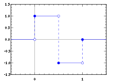
β​(x)={1, 0≀x<12βˆ’1,12≀x<10,otherwise𝛽π‘₯casesmissing-subexpression1 0π‘₯12missing-subexpressionmissing-subexpression112π‘₯1missing-subexpressionmissing-subexpression0otherwisemissing-subexpression\displaystyle\beta(x)=\left\{\begin{array}[]{lll}&1,\leavevmode\nobreak\ \leavevmode\nobreak\ 0\leq x<\frac{1}{2}\\ &-1,\leavevmode\nobreak\ \leavevmode\nobreak\ \frac{1}{2}\leq x<1\\ &0,\leavevmode\nobreak\ \leavevmode\nobreak\ \text{otherwise}\end{array}\right. (45)

and,

β​(2​x)={1, 0≀x<14βˆ’1,14≀x<120,otherwise𝛽2π‘₯casesmissing-subexpression1 0π‘₯14missing-subexpressionmissing-subexpression114π‘₯12missing-subexpressionmissing-subexpression0otherwisemissing-subexpression\displaystyle\beta(2x)=\left\{\begin{array}[]{lll}&1,\leavevmode\nobreak\ \leavevmode\nobreak\ 0\leq x<\frac{1}{4}\\ &-1,\leavevmode\nobreak\ \leavevmode\nobreak\ \frac{1}{4}\leq x<\frac{1}{2}\\ &0,\leavevmode\nobreak\ \leavevmode\nobreak\ \text{otherwise}\end{array}\right. (49)
β​(2​xβˆ’1)=β​(2​(xβˆ’12))={1,12≀x<34βˆ’1,34≀x<10,otherwise𝛽2π‘₯1𝛽2π‘₯12casesmissing-subexpression112π‘₯34missing-subexpressionmissing-subexpression134π‘₯1missing-subexpressionmissing-subexpression0otherwisemissing-subexpression\displaystyle\beta(2x-1)=\beta(2(x-\frac{1}{2}))=\left\{\begin{array}[]{lll}&1,\leavevmode\nobreak\ \leavevmode\nobreak\ \frac{1}{2}\leq x<\frac{3}{4}\\ &-1,\leavevmode\nobreak\ \leavevmode\nobreak\ \frac{3}{4}\leq x<1\\ &0,\leavevmode\nobreak\ \leavevmode\nobreak\ \text{otherwise}\end{array}\right. (53)

ΦΦ\Phi constitutes an orthonormal bases in L2​(ℝ)superscript𝐿2ℝL^{2}(\mathbb{R}). FigureΒ 1 shows a plot of standard Haar wavelet β​(x)𝛽π‘₯\beta(x).

Refer to caption
Figure 1: Haar Wavelet, β​(x)𝛽π‘₯\beta(x)

The connection of polynomial bases and Haar wavelet is shown in TableΒ 2. Ο†0,ksubscriptπœ‘0π‘˜\varphi_{0,k} is a coarse scale representation, while ψj,ksubscriptπœ“π‘—π‘˜\psi_{j,k} is a finer scale representation. In high dimension, tensor product will be used.

Table 2: Connection of Polynomial Chaos (PC) and the wavelet basis
Legendre polynomial wavelet basis wavelet expression
with variable z𝑧z
1 Ο†0,ksubscriptπœ‘0π‘˜\varphi_{0,k} Ο‡[0,1)​(zβˆ’k)subscriptπœ’01π‘§π‘˜\chi_{[0,1)}(z-k)
z𝑧z ψ0,ksubscriptπœ“0π‘˜\psi_{0,k} c0​β​(zβˆ’k)subscript𝑐0π›½π‘§π‘˜c_{0}\beta(z-k)
32​z232superscript𝑧2\frac{3}{2}z^{2} ψ1,ksubscriptπœ“1π‘˜\psi_{1,k} c1​β​(2​zβˆ’k)subscript𝑐1𝛽2π‘§π‘˜c_{1}\beta(2z-k)
β‹―β‹―\cdots β‹―β‹―\cdots β‹―β‹―\cdots

Projecting a variable Z𝑍Z onto the wavelet basis, we have

Z=βˆ‘kβˆˆβ„€<Z,Ο†0,k>Ο†0,k+βˆ‘j=0βˆžβˆ‘kβˆˆβ„€<Z,ψj,k>ψj,kformulae-sequence𝑍subscriptπ‘˜β„€π‘subscriptπœ‘0π‘˜subscriptπœ‘0π‘˜superscriptsubscript𝑗0subscriptπ‘˜β„€π‘subscriptπœ“π‘—π‘˜subscriptπœ“π‘—π‘˜\displaystyle Z=\sum\limits_{k\in\mathbb{Z}}<Z,\varphi_{0,k}>\varphi_{0,k}+\sum\limits_{j=0}^{\infty}\sum\limits_{k\in\mathbb{Z}}<Z,\psi_{j,k}>\psi_{j,k} (54)

Considering the wavelet with n𝑛n vanishing moment, that is

βˆ«βˆ’βˆžβˆžzkβ€‹Οˆβ€‹(z)​𝑑z=0,(0≀k<n),superscriptsubscriptsuperscriptπ‘§π‘˜πœ“π‘§differential-d𝑧00π‘˜π‘›\displaystyle\int_{-\infty}^{\infty}z^{k}\psi(z)dz=0,\leavevmode\nobreak\ \leavevmode\nobreak\ (0\leq k<n), (55)

when n=2𝑛2n=2, we have βˆ«βˆ’βˆžβˆžzβ€‹Οˆβ€‹(z)​𝑑z=0superscriptsubscriptπ‘§πœ“π‘§differential-d𝑧0\int_{-\infty}^{\infty}z\psi(z)dz=0, and βˆ«βˆ’βˆžβˆžz2β€‹Οˆβ€‹(z)​𝑑z=0superscriptsubscriptsuperscript𝑧2πœ“π‘§differential-d𝑧0\int_{-\infty}^{\infty}z^{2}\psi(z)dz=0. (We can express it in the form of Daubechies wavelet, although there is no explicit expression for the wavelet terms Οˆπœ“\psi. Haar wavelet has an explicit expression.) Referring to the polynomial case, we can use wavelet to express the equation terms, for example: ei​p​q​j=𝔼​(Ξ¦i​Φp​Φq​Φj)=βˆ«Ο†0,k​(z)β€‹Οˆj,k​(z)​φ0,k​(z)​φ0,k​(z)​ρ​(z)​𝑑zsubscriptπ‘’π‘–π‘π‘žπ‘—π”ΌsubscriptΦ𝑖subscriptΦ𝑝subscriptΞ¦π‘žsubscriptΦ𝑗subscriptπœ‘0π‘˜π‘§subscriptπœ“π‘—π‘˜π‘§subscriptπœ‘0π‘˜π‘§subscriptπœ‘0π‘˜π‘§πœŒπ‘§differential-d𝑧e_{ipqj}=\mathbb{E}(\Phi_{i}\Phi_{p}\Phi_{q}\Phi_{j})=\int\varphi_{0,k}(z)\psi_{j,k}(z)\varphi_{0,k}(z)\varphi_{0,k}(z)\rho(z)dz. When the parameters of uncertainty is high dimension, the computation is still difficult.

5 Perturbation method

When Z∈(0,Ξ΄)𝑍0𝛿Z\in(0,\delta) is a random variable, and Ξ΄<<1much-less-than𝛿1\delta<<1. The initial condition is uncertain, and can be written as

u0​(x,y,Z)=u​(x,y,0,Z)=u0​(x,y)+Zsuperscript𝑒0π‘₯𝑦𝑍𝑒π‘₯𝑦0𝑍superscript𝑒0π‘₯𝑦𝑍\displaystyle u^{0}(x,y,Z)=u(x,y,0,Z)=u^{0}(x,y)+Z

In the perturbative approach, the stochastic quantities are expanded via a Taylor series around the mean value of the random inputs,

u0​(x,y,Z)=u​(x,y,0,Z)=u00​(x,y)+Z​u10​(x,y)+β‹―superscript𝑒0π‘₯𝑦𝑍𝑒π‘₯𝑦0𝑍superscriptsubscript𝑒00π‘₯𝑦𝑍superscriptsubscript𝑒10π‘₯𝑦⋯\displaystyle u^{0}(x,y,Z)=u(x,y,0,Z)=u_{0}^{0}(x,y)+Zu_{1}^{0}(x,y)+\cdots (56)

where

uk​(x,y,t)=k!β€‹βˆ‚ku​(x,y,t,Z)βˆ‚kZsubscriptπ‘’π‘˜π‘₯π‘¦π‘‘π‘˜superscriptπ‘˜π‘’π‘₯𝑦𝑑𝑍superscriptπ‘˜π‘\displaystyle u_{k}(x,y,t)=k!\frac{\partial^{k}u(x,y,t,Z)}{\partial^{k}Z}

the expansion is at the point of the mean of the distribution. Substituting expansionΒ (56) into the Cahn-Hilliard equationΒ (13), and equating the terms of different orders, under the assumption that O​(1)>>O​(Z)>>O​(Z2)>>β‹―much-greater-than𝑂1𝑂𝑍much-greater-than𝑂superscript𝑍2much-greater-thanβ‹―O(1)>>O(Z)>>O(Z^{2})>>\cdots, and the condition that u00=u0superscriptsubscript𝑒00subscript𝑒0u_{0}^{0}=u_{0}, u10=1superscriptsubscript𝑒101u_{1}^{0}=1, and uk0=0superscriptsubscriptπ‘’π‘˜00u_{k}^{0}=0 for kβ‰₯2π‘˜2k\geq 2, we have

O(Z0):βˆ‚u0βˆ‚t=βˆ’Ξ”(ΡΔu0βˆ’1Ξ΅(4u03βˆ’6u02+2u0))+Ξ»(fβˆ’u0)\displaystyle O(Z^{0}):\leavevmode\nobreak\ \leavevmode\nobreak\ \frac{\partial u_{0}}{\partial t}=-\Delta(\varepsilon\Delta u_{0}-\frac{1}{\varepsilon}(4u_{0}^{3}-6u_{0}^{2}+2u_{0}))+\lambda(f-u_{0}) (57)
O(Z1):βˆ‚u1βˆ‚t=βˆ’Ξ”(ΡΔu1βˆ’1Ξ΅(4β‹…(3u02u1)βˆ’6(2u0u1)+2u1))βˆ’Ξ»u1\displaystyle O(Z^{1}):\leavevmode\nobreak\ \leavevmode\nobreak\ \frac{\partial u_{1}}{\partial t}=-\Delta(\varepsilon\Delta u_{1}-\frac{1}{\varepsilon}(4\cdot(3u_{0}^{2}u_{1})-6(2u_{0}u_{1})+2u_{1}))-\lambda u_{1} (58)

6 Experiments

As shown inΒ [3], the effect of using binary Cahn-Hilliard equation for image inpainting is shown in FigureΒ 2.

Refer to caption
(a) Masked image
Refer to caption
(b) Output image
Figure 2: Binary image inpainting

For Gaussian noise case, that is ZβˆΌπ’©β€‹(0,1)similar-to𝑍𝒩01Z\sim\mathcal{N}(0,1), with probability density function

ρ​(z)=12​π​eβˆ’z2/2,πœŒπ‘§12πœ‹superscript𝑒superscript𝑧22\displaystyle\rho(z)=\frac{1}{\sqrt{2\pi}}e^{-z^{2}/2}, (59)

applying the Stochastic Galerkin method for Cahn-Hilliard equation. According to TableΒ 1, and the orthogonality conditionΒ 3.3, the hermite orthogonal polynomial {Hm​(Z)}subscriptπ»π‘šπ‘\{H_{m}(Z)\}:

H0​(Z)=1,H1​(Z)=Z,H2​(Z)=Z2βˆ’1,H3​(Z)=Z3βˆ’3​Z,β‹―formulae-sequencesubscript𝐻0𝑍1formulae-sequencesubscript𝐻1𝑍𝑍formulae-sequencesubscript𝐻2𝑍superscript𝑍21subscript𝐻3𝑍superscript𝑍33𝑍⋯\displaystyle H_{0}(Z)=1,\leavevmode\nobreak\ \leavevmode\nobreak\ \leavevmode\nobreak\ H_{1}(Z)=Z,\leavevmode\nobreak\ \leavevmode\nobreak\ \leavevmode\nobreak\ H_{2}(Z)=Z^{2}-1,\leavevmode\nobreak\ \leavevmode\nobreak\ \leavevmode\nobreak\ H_{3}(Z)=Z^{3}-3Z,\leavevmode\nobreak\ \cdots

is used as the basis function.

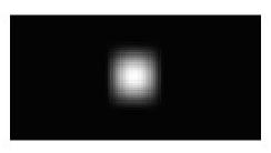
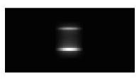
Applying the stochastic Galerkin method, we can obtain the mean and first order solution of u𝑒u, as shown in FigureΒ 3.

Refer to caption
(a) Mean image of the final stage
Refer to caption
(b) Mean image of the final stage
Figure 3: Image inpainting with stochastic Galerkin method

According to perturbation method, the mean solution and the first order solution are shown in FigureΒ 4.

Refer to caption
(a) Plot of leading order solution of the final stage
Refer to caption
(b) First order solution of the final stage
Figure 4: Image inpainting with perturbation expansion

References

  • [1] D. Xiu. Numerical Method for Stochastic Computations: A Spectral Method Approach (Princeton University Press, 41 William Street, NJ), pp. 30-32 (2010).
  • [2] J. Hu, S. Jin, and D. Xiu. β€œA Stochastic Galerkin Method for Hamilton-Jacobi Equation with Uncertainty,” SIAM J. SCI. COMPUT. 37, A2246-A2269 (2015).
  • [3] A. Bertozzi, S. Esedoglu, and A. Gillette. β€œInpainting of Binary Images Using the Cahn-Hilliard Equation,” IEEE Transaction on Image Processing 16, 285-291 (2007).
  • [4] J. Bosch. β€œFast Iterative Solvers for Cahn-Hilliard Problems.” PhD dissertation, Otto-von-Guericke UniversitΓ€t Magdeburg, 2016.
  • [5] D. Xiu and G. Karniadakis. β€œSupersensitivity due to uncertain boundary conditions,” International journal for numerical methods in Engineering 61, 2114-2138 (2004).
  • [6] C. Schonlieb. Partial Differential Equation Methods for Image Inpainting(Cambridge University Press)