Buoyancy-Driven Entrainment in Dry Thermals

Abstract

Turner, (1957) proposed that dry thermals entrain because of buoyancy (via a constraint which requires an increase in the radius $a$). This however, runs counter to the scaling arguments commonly used to derive the entrainment rate, which rely on either the self-similarity of Scorer, (1957) or the turbulent entrainment hypothesis of Morton et al., (1956). The assumption of turbulence-driven entrainment was investigated by Lecoanet and Jeevanjee, (2018), who found that the entrainment efficiency $e$ varies by less than $20\%$ between laminar (Re = 630) and turbulent (Re = 6300) thermals. This motivated us to utilize Turner’s argument of buoyancy-controlled entrainment in addition to the thermal’s vertical momentum equation to build a model for thermal dynamics which does not invoke turbulence or self-similarity. We derive simple expressions for the thermals’ kinematic properties and their fractional entrainment rate $\epsilon$ and find close quantitative agreement with the values in direct numerical simulations. In particular, our expression for entrainment rate is consistent with the parameterization $\epsilon\sim B/w^{2}$, for Archimedean buoyancy $B$ and vertical velocity $w$. We also directly validate the role of buoyancy-driven entrainment by running simulations where gravity is turned off midway through a thermal’s rise. The entrainment efficiency $e$ is observed to drop to less than 1/3 of its original value in both the laminar and turbulent cases when $g=0$, affirming the central role of buoyancy in entrainment in dry thermals.

Keywords— Convection; Turbulence; Theory; Buoyancy; Atmosphere; Vorticity; Baroclinicity; Entrainment

Funding Information

BM is supported by the NOAA Hollings Scholarship, DL is supported by a PCTS fellowship and a Lyman Spitzer Jr. fellowship, and NJ is supported by a Harry Hess fellowship from the Princeton Geoscience Department. Computations were conducted with support by the NASA High End Computing (HEC) program through the NASA Advanced Supercomputing (NAS) Division at Ames Research Center on Pleiades, as well as GFDL’s computing cluster.

1   Introduction

Since the introduction of the entrainment hypothesis by Morton et al., (1956), the physical mechanism of entrainment has been thought to originate from turbulent eddies. The wide acceptance of this theory is due to its success in analyzing flows such as jets and plumes in a large variety of physical contexts (Turner,, 1986). The entrainment hypothesis states that the average inflow velocity across the edge of a turbulent flow is assumed to be proportional to a characteristic velocity. There are some flows however, where entrainment persists even in the laminar regime. For instance, “thermals”, or regions of isolated buoyant fluid thought to be the basic unit of convection (Romps and Charn,, 2015; Yano,, 2014), were recently found to vary in entrainment by less than 20% in laminar (Re = 630) and turbulent (Re = 6300) simulations in a dry atmosphere (Lecoanet and Jeevanjee,, 2018).

The observed expansion rates in thermals is much larger than that of plumes and is sensitive to the initial conditions (Turner,, 1986; Turner et al.,, 1973). According to Turner, (1957), these properties may be better understood if the thermal is modeled as a buoyant vortex ring. Turner, (1957) shows why a buoyant ring must expand with time due to momentum conservation, and an illuminating, complementary perspective was provided by Zhao et al., (2013) which shows that a ring’s expansion is related to its baroclinicity. We refer the reader to Zhao et al., (2013) for a more in-depth explanation.

Here, we combine the buoyant vortex ring argument of Turner, (1957) with the thermal’s vertical momentum equation by regarding the thermal as the region of fluid that moves coherently with the vortex ring (i.e. as the ellipsoidal region of fluid whose average velocity equals the gross translational velocity of the vortex ring itself). This aligns with the notion of a vortex ring “bubble” (Akhmetov,, 2009; Shariff and Leonard,, 1992), and we assume that the radius of the thermal $a$ is proportional to the radius of the vortex $R$, ie. $a=\xi R$. Utilizing this connection, we derive analytical expressions for the density, vertical velocity, height, and radius as functions of time. We then relate the radius to the height to get an expression for the fractional entrainment rate, $\epsilon\equiv\frac{d\log V}{dz}=e/a$, where $e$ is a proportionality constant called the “entrainment efficiency” and $a$ is the radius of the thermal. This is significant because our predictions require no tuning parameters to fit the data, unlike previous works, (Johari,, 1992; Turner,, 1986; Simpson,, 1983; Escudier and Maxworthy,, 1973; Simpson and Wiggert,, 1969; Turner,, 1964, 1962; Levine,, 1959; Morton et al.,, 1956). We validate this model by comparing the predictions of the radius, height, density, vertical velocity, and fractional entrainment to direct numerical simulations of dry thermals.

Our model does not invoke turbulence, contrary to the substantial amount of literature which attributes entrainment in convection to turbulent eddies (Yano,, 2014; de Rooy et al.,, 2013; Sherwood et al.,, 2013; de Rooy and Siebesma,, 2010; Romps and Kuang,, 2010; Craig and Dörnbrack,, 2008; Ferrier and Houze,, 1989; Baker et al.,, 1984; Escudier and Maxworthy,, 1973; Turner,, 1964; Morton et al.,, 1956). In addition to validating our simple non-turbulent model against simulation data, we directly test the role of buoyancy by performing numerical simulations where gravity is removed midway through a thermal’s rise. The thermals’ observed entrainment rates decrease significantly. Our expressions and simulations seem to indicate that entrainment in dry thermals is predominantly a laminar process, consistent with Sànchez et al., (1989) and contravening the original entrainment hypothesis. Furthermore, buoyancy-driven entrainment is distinct from the ‘dynamic’ entrainment proposed in Houghton and Cramer, (1951) and used in Morrison, (2017); de Rooy and Siebesma, (2010); Ferrier and Houze, (1989); Asai and Kasahara, (1967), since dynamic entrainment is a consequence of positive vertical acceleration, whereas our theory and simulations show negative vertical acceleration. We conclude with a discussion of the implications of these findings on future studies of entrainment, given the importance of this process in understanding cumulus convection and climate sensitivity (Zhao,, 2014; Klocke et al.,, 2011).

We begin by reviewing previous work on buoyant vortex rings in section 2 and discuss the relationship between a vortex ring and a thermal. In section 3 we introduce a new model which allows us to derive the characteristics of a thermal and its entrainment. In section 4 we verify the predictions made by the model and then affirm the role of buoyancy in entrainment. In section 5 we discuss second order contributions to entrainment and conclude by looking at future research directions.

2   The Physics of Buoyant Vortex Rings

2.1  Fundamental Fluid Mechanics

In our analysis of thermals we will use the Boussinesq approximation to the momentum equation, where density differences $\rho^{\prime}$ in the flow are small compared to the constant background reference density $\bar{\rho}$. We decompose the density as $\rho=\bar{\rho}+\rho^{\prime}$. The pressure can be decomposed similarly as $p=\bar{p}+p^{\prime}$ where $\bar{p}$ is in hydrostatic balance with $\bar{\rho}$, ie. $\nabla\bar{p}=\bar{\rho}\bm{g}$, where $\bm{g}=-g\bm{\hat{z}}$ is the gravitational acceleration. Formally, the Boussinesq approximation is valid when vertical length scales in the problem are smaller than the scale height. This approximation is helpful, as it eliminates the effect of adiabatic expansion of a fluid parcel as it rises. Therefore, the observed expansion of thermals will be purely due to the mechanical effect of entrainment. The integrated buoyancy force in the Boussinesq approximation is $F=-\int\rho^{\prime}g\ dV$, where the integral is taking over the region of interest. The momentum equation is $\frac{D\bm{u}}{Dt}=\frac{1}{\bar{\rho}}\big{[}\rho^{\prime}\bm{g}-\nabla{p^{\prime}}\big{]}+\nu\nabla^{2}\bm{u}$, where $\bm{u}$ is the velocity field and $\nu$ is the kinematic viscosity.

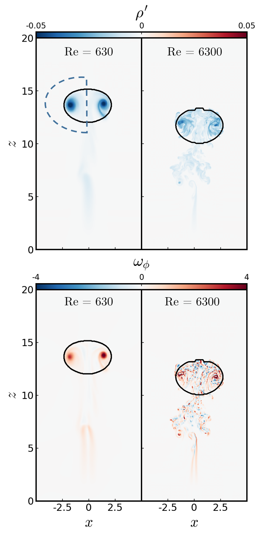
Figure 1: 2D vertical slices at the thermal midpoint of the density perturbation (top) and vorticity (bottom) of two thermals with different Reynolds numbers at $\tau=2.5$. The left (right) panel shows the Re=630 (Re=6300) simulations. The same color scale is used for both Re. The thermals originally start as a buoyant sphere (with noise added to break the symmetries of the problem), but then develop into a vortex ring that induces a flow structure that moves coherently with it. We identify this region as the thermal, and details of how it is computed is given Lecoanet and Jeevanjee, (2018), section 3. The contour of the thermal is plotted in black. Both the density perturbations and the vorticity become primarily concentrated within the core region of the vortex in the laminar thermal. This is also true in the turbulent thermal, but to a lesser extent due to vorticity fluctuations at many scales, characteristic of a turbulent fluid. The dashed blue line is an example of a circuit $\partial\mathcal{S}$ which passes through no buoyant fluid and can be used for Eqn. (1) and Eqn. (3).

Figure 2: Azimuthally averaged vertical slices of the change in vorticity $\langle\frac{D\omega_{\phi}}{Dt}\rangle$ at $\tau=2.5$. Angle brackets denote an azimuthal average has been taken, which is the reason for the symmetry of the figures across $x=0$. Radial gradients in the density field produce a torque (baroclinicity) that drives the continual destruction of vorticity in the center of the vortex and the continual creation vorticity in the outer region. This causes the center of rotation of the vortex to continually move outward (Zhao et al.,, 2013) and is the mechanical description of how dry thermals expand and therefore entrain as they rise.

When a spherical thermal is released from rest, it accrues vorticity from its baroclinicity and generates a vortex ring structure, where density perturbations $\rho^{\prime}$ are largely confined to the vortex core that develops, Figure 1. Buoyancy is present only where there are density perturbations, therefore, the buoyancy resides mostly within the vortex core. In our model, we will assume that the buoyancy resides entirely within the vortex core. This assumption will be tested in Section 4. We introduce some basic aspects of vortex rings below.

2.2  Vortex Ring Dynamics

A vortex ring can be characterized by its kinematic properties such as circulation and impulse. The circulation of a vortex ring can be calculated along a circuit $\partial\mathcal{S}$ passing through the center of the thermal’s vortex ring and then returning through the ambient fluid, like in Figure 1. The integral can also be computed as an area integral of vorticity over the region bounded by the circuit, $\mathcal{S}$. For vortex rings, which are azimuthally symmetric, the vorticity is $\bm{\omega}=\omega_{\phi}\bm{\hat{\phi}}$ and this integral simplifies in cylindrical coordinates $(r,\phi,z)$, where the origin is located in the center of the vortex ring,

$$\Gamma\ \equiv\ \oint_{\partial\mathcal{S}}\bm{u}\cdot d\bm{l}\ =\ \int_{\mathcal{S}}\omega_{\phi}\ \ drdz\ .$$ (1)

The impulse for incompressible fluids is defined as (Shivamoggi,, 2010; Akhmetov,, 2009; Batchelor,, 2000; Lamb and Caflisch,, 1993),

$$\bm{I}\ \equiv\ \frac{1}{2}\rho\int_{\mathcal{V}}\bm{x}\times\bm{\omega}\quad dV\ ,$$ (2)

where $\bm{x}$ is the position vector and $\mathcal{V}$ is the entire domain. It can be interpreted as the time and volume integral of external forces that must be applied to a flow in order to generate the observed fluid motion from rest (Lamb and Caflisch,, 1993). Therefore, internal forces such as pressure or viscosity do not come into play. Eqn. (2) simplifies if we assume the flow is Boussinesq, that the radius of the core is much smaller than the radius of the ring $R$, and use the second part of Eqn. (1),

$$I_{z}\ =\ \pi\bar{\rho}\ \Gamma R^{2}\ .$$ (3)

We only get an impulse in the z direction, which is a consequence of the azimuthal symmetry of the flow. We turn to the circulation equation to consider how circulation evolves in time,

$$\frac{d\Gamma}{dt}=\int_{\mathcal{S}}\bigg{(}\frac{\nabla\rho^{\prime}\times\bm{g}}{\bar{\rho}}+\text{Re}^{-1}\nabla^{2}\bm{\omega}\bigg{)}\cdot d\bm{A}$$ (4)

In our current analysis we will assume the Reynolds number is sufficiently high that the viscous effects can be neglected (though see section 5.1 for more discussion of viscous torques). If the circuit $\partial\mathcal{S}$ passes through no buoyant fluid, then the circulation is constant with time (Fohl,, 1967). This circuit will be possible once the vortex ring has formed, so we expect the circulation to initially increase with time as the thermal “spins up” but then reach a constant value. We will verify this property of the circulation in section 4.

2.3  Expansion by Conservation of Momentum

Turner, (1957)’s argument applies after the vortex ring reaches a constant circulation and can be summarized succinctly: Internal forces such as pressure or viscosity do not affect the impulse of the ring, so the change in impulse only depends on buoyancy.

$$\frac{dI_{z}}{dt}\ =\ \pi\bar{\rho}\ \Gamma\frac{dR^{2}}{dt}\ =\ F\ >\ 0\ .$$ (5)

$F$ and $\bar{\rho}$ are constants and therefore $R$ must increase with time, i.e. the thermal must entrain. For a generalization of this argument to the density-stratified case where $\bar{\rho}$ is not constant, see Anders et al., (2019).

2.4  Expansion by Baroclinicity

Although the argument in Eqn. (5) shows why the radius of thermal increases with time, it is helpful to look at the vorticity equation to explain how. We follow Zhao et al., (2013) below. The vorticity equation in the Boussinesq approximation is,

$$\frac{D\bm{\omega}}{Dt}\ =\ (\bm{\omega}\cdot\nabla)\bm{u}\ +\ \frac{\nabla\rho^{\prime}\times\bm{g}}{\bar{\rho}}\ +\ \text{Re}^{-1}\nabla^{2}\bm{\omega}\ .$$ (6)

Once again ignoring viscous effects, in cylindrical coordinates we have

$$\frac{D\omega_{\phi}}{Dt}\ =\ u_{r}\frac{\omega_{\phi}}{r}\ +\ \frac{g}{\bar{\rho}}\frac{\partial\rho^{\prime}}{\partial r}\ .$$ (7)

The first term represents the intensification of vorticity due to stretching of vortex lines (Thorne and Blandford,, 2017), but should disappear when integrated over the entire thermal because of the symmetry of the field, Figures 1 and 2. Equation (7) then tells us that the vorticity evolution is dictated by the second term, baroclinicity, which depends on gradients in density perturbations. The gradients are always set up such that vorticity is constantly being created in the exterior of the ring and destroyed in the interior, as shown in Figure 2, and thus the core region of the ring appears to continually move radially outward. As the ring expands, it entrains more fluid. This will be shown to be the dominant mechanism of entrainment in section 4.

3   A New Model for Thermals

Figure 3: Verification of constant circulation $\Gamma$ for laminar (yellow) and turbulent (purple) simulations. For both cases, $\Gamma$ is roughly constant, which validates the approximation used to derive Eqn. (11). The circulation also shows the thermals’ spin up periods. We chose our timescale such that $\tau=1$ is approximately the spin up time.

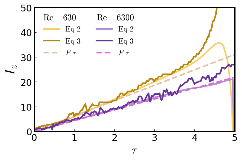
Figure 4: Verification of impulse expressions. The laminar thermal’s impulse is shown in yellow and the turbulent’s in purple. Equation (3) was derived assuming the radius of the core region of a vortex is small compared to its overall radius. We test the validity of this assumption by explicitly comparing it to the impulse computed by Eqn. (2). We also assume integrated buoyancy is constant and therefore the impulse generated by it, $F\tau$, can be calculated too. We find that in both laminar and turbulent thermals, $F\tau$ tracks Eqn. (2) closely.

Given the above picture for buoyancy-driven entrainment in thermals, we endeavour to build an analytical model for thermals which captures this picture, inspired by the formulation of Escudier and Maxworthy, (1973) who invoke the vertical momentum equation. In particular, we assume:

1. The flow is Boussinesq and begins as a buoyant sphere at $t=0$, but then fully spins up into a vortex ring at $t=t_{o}$ with radius $R_{o}$, height $z_{o}$, and vertical velocity $w_{o}$.

2. The impulse of a buoyant vortex ring is given by Eqn. (3), with circulation $\Gamma$ and background density $\bar{\rho}$ being constant.

3. The only external force imparting an impulse is the integrated buoyancy $F$, which is constant because detrainment is assumed to be negligible (Lecoanet and Jeevanjee,, 2018). The Gross entrainment doesn’t affect $F$ because the surrounding fluid has no mass anomaly. While $\langle\rho^{\prime}\rangle$ will change and $V$ will change, their combination $\langle\rho^{\prime}\rangle V$ will remain constant. For a thermal with volume $V=ma^{3}$,

   $$F\ =\ ma^{3}\big{<}\rho^{\prime}\big{>}g\ =\ \text{constant},$$ (8)

   where $\big{\langle}\rho^{\prime}\big{\rangle}$ is the average density anomaly of the thermal and $m$ is a constant for the volume since the thermal is no longer a sphere. $m$ is verified to be roughly constant in Anders et al., (2019).

4. The thermal is the region of fluid that moves coherently with the vortex ring and so the thermal’s radius $a$ is proportional to the vortex radius $R$, ie. $a=\xi R$.

5. The impulse of a thermal with volume $ma^{3}$ and vertical velocity $w$ can be written as (Akhmetov,, 2009),

   $$I_{z}\ =\ ma^{3}\bar{\rho}(1+k)w\ ,$$ (9)

   where we parameterize virtual mass effects via a virtual mass coefficient $(1+k)$ (Batchelor,, 2000). For all ellipsoidal fluid geometries, the value of $k$ is the same as the solid body value of the same geometry, Tarshish et al., (2018).

These assumptions will be discussed in more detail throughout the rest of the paper and will be tested along with the model predictions in section 4.

We begin our analysis with the vortex momentum equation (3) which is equal to the impulse imparted by the integrated buoyancy, $Ft$. Assuming that $F$ is constant, we evaluate this equality at $t$ and $t_{o}$ and take their ratio to get the radius of the vortex ring as a function of time,

$$\begin{split}R(t)\ &=\ R_{o}\sqrt{t/t_{o}}\ .\\ \end{split}$$ (10)

We utilize the proportionality of $a$ and $R$ and introduce a nondimensional time, $\tau=t/t_{o}$ to get the thermal’s radius.

$$a(\tau)\ =\ a_{o}\sqrt{\tau}\ .$$ (11)

Now consider the equation for integrated buoyancy conservation, (8). If we plug in Eqn. (11) for $a$, we can solve for $\big{<}\rho^{\prime}\big{>}$ explicitly as a function of time,

$$\big{<}\rho^{\prime}\big{>}(\tau)\ =\ \frac{\big{<}\rho^{\prime}_{o}\big{>}}{\tau^{3/2}}\ ,$$ (12)

where $\langle\rho_{o}^{\prime}\rangle$ is the average density anomaly of the thermal at $t_{o}$. Now we turn to the Boussinesq momentum equation for a spherical thermal, (9). In this formulation, a thermal is the region of fluid moving together with the vortex, so the impulse will be equal to the sum of the vortex momentum and the momentum created by virtual mass (Akhmetov,, 2009). Evaluating Eqn. (9) at $t$ and $t_{o}$ and taking their ratio gives the velocity of the thermal as a function of time,

$$\begin{split}w(\tau)\ &=\ w_{o}/\sqrt{\tau}\ .\end{split}$$ (13)

Now we integrate $w$ to get $z$.

$$\begin{split}z(\tau)\ &=\ z_{o}\ +\ 2w_{o}t_{o}\big{(}\sqrt{\tau}-1\big{)}\ .\end{split}$$ (14)

Assuming that detrainment is negligible implies that integrated buoyancy is conserved. Therefore the fractional entrainment rate is also the fractional change in thermal volume with respect to height (Lecoanet and Jeevanjee,, 2018). Straight forward algebra shows $\epsilon=\frac{d\log V}{dz}=\frac{3}{a}\frac{da}{dz}$. Expressed as a function of the thermal’s radius,

$$\begin{split}\epsilon(a)\ &=\ \frac{3a_{o}}{2w_{o}t_{o}}\frac{1}{a}\ .\end{split}$$ (15)

This is one of the main results of this paper, along with having an analytical model for all the thermal’s variables ($a,w,\langle\rho^{\prime}\rangle$) which does not invoke similarity or turbulence. Unlike Escudier and Maxworthy, (1973), our approach does not require any additional empirical constants to determine the thermal’s behavior. This is because Escudier and Maxworthy, (1973) use the turbulent entrainment assumption, $\frac{d(\rho a^{3})}{dt}=3\alpha\bar{\rho}a^{2}\lvert w\rvert$, ($\alpha$ is an unspecified constant tuned to match experiments), instead of Eqn. (3). They now have 4 unknowns ($a$,$w$,$\langle\rho^{\prime}\rangle$,$\alpha$) and only 3 equations. In our case however, we employ (3) instead of an entrainment assumption to fully solve the system for $a$, $w$, and $\langle\rho^{\prime}\rangle$.

Our approach also gives a simple expression for the thermal’s entrainment efficiency,

$$\begin{split}e\ &=\ \frac{3a_{o}}{2w_{o}t_{o}}\ .\end{split}$$ (16)

We can also use (3), (9), and $I_{z}=Ft$ to rewrite the efficiency in terms of the thermal’s integrated buoyancy and circulation. This yields another key result, namely that $e$ is a constant dictated by the initial spin up of the thermal:

$$e\ =\ \frac{3m(1+k)F\xi^{4}}{2\pi^{2}\bar{\rho}\Gamma^{2}}\ .$$ (17)

Thermals with different initial conditions will thus have different efficiencies, which perhaps explains the variance of efficiencies with respect to Re found in Lecoanet and Jeevanjee, (2018). Equation (17) suggests in particular that differences in $e$ between the laminar and turbulent cases in that paper may stem from differences in $\Gamma$ (Figure 3 below). Furthermore, variations in initial aspect ratio, which Lai et al., (2015) showed could explain the large range of thermal entrainment rates found in the literature, might also be understood via (17) in terms of their effect on $F$ and $\Gamma$.

Figure 5: Verification of theory for thermal’s (a)(b) radius $a$, (c)(d) cloud top height $z$, and (e)(f) average density perturbation $\langle\rho^{\prime}\rangle$. All values are normalized by their spin up value at $\tau=1$. The predicted values from Eqns. (11), (14), and (12) are the dashed lines and simulation values are the solid lines for the laminar (yellow) and turbulent (purple) cases. The deviations in the laminar data for $\tau>3.5$ is due to the thermal interacting with the top boundary. We find that both thermals exhibit power law behavior, consistent with Lecoanet and Jeevanjee, (2018).

Figure 6: Verification of entrainment theory. Plotted is the fractional entrainment rate $\epsilon$ as a function of thermal radius $a$. Predicted values from Eqn. (15) are dashed lines and simulation data are solid lines. Our model accurately predicts the entrainment rate in both laminar and turbulent simulations, although deviations are slightly larger in the turbulent case. Note the similarity in $\epsilon$ between laminar and turbulent simulations. Deviations occur for the laminar simulation at $a>2.7$, because the thermal starts to interact with the top boundary.

Another important aspect of (17) is that it embodies the well-known scaling $e\sim\frac{F}{\bar{\rho}\Gamma^{2}}$ (e.g. Lai et al.,, 2015; Bond and Johari,, 2010; Fohl,, 1967; Turner,, 1957). If we apply this scaling to the entrainment rate $\epsilon$ and write it using $\Gamma\sim wa$ and $F\sim\bar{\rho}Ba^{3}$ (where $B=g\langle\rho^{\prime}\rangle/\bar{\rho}$ is the average Archimedean buoyancy), we find

$$\epsilon\sim\frac{B}{w^{2}}\ .$$ (18)

Though this scaling is not often applied to atmospheric convection, it was recently employed (on largely dimensional grounds) in the parameterization of Tan et al., (2018), and was also used in Gregory, (2001). Equation (17) provides a precise foundation for (18), at least in the idealized dry case.

4   Verification of the Model

4.1  Simulation Setup

We analyze the direct numerical simulations of thermals found in Lecoanet and Jeevanjee, (2018). We outline the simulation setup below, but for more details (including the scalings used for nondimensionalization), see section 2 of Lecoanet and Jeevanjee, (2018). Simulations are run with Dedalus, an open source pseudo-spectral framework (Burns et al.,, 2019). We solve the non-dimensionalized Boussinesq equations:

$$\partial_{t}\bm{u}+\nabla p-\mathrm{Re}^{-1}\nabla^{2}\bm{u}+\rho^{\prime}\bm{e_{z}}\ =\ -\bm{u}\cdot\nabla\bm{u}$$ (19a)

$$\partial_{t}\rho^{\prime}\ -\ \mathrm{Pr}^{-1}\mathrm{Re}^{-1}\nabla^{2}\rho^{\prime}\ =\ -\bm{u}\cdot\nabla\rho^{\prime}$$ (19b)

$$\nabla\cdot\bm{u}\ =\ 0$$ (19c)

After non-dimensionalization, the simulations are entirely described by the initial condition, the Reynolds number and the Prandtl number. We take $\text{Pr}=1$ for all simulations, $\text{Re}=630$ for laminar runs, and $\text{Re}=6300$ for turbulent runs.

We initialize the thermal with a spherical density anomaly $\rho^{\prime}$ of magnitude negative $1$ and diameter $L_{th}$, plus a noise field to break symmetries in the problem. The spherical anomaly is placed near the bottom of a 3D domain with height $20L_{th}$ and horizontal lengths $10L_{th}$. The simulation time ranges from $t\in[0,63.2]$, long enough for the thermal to approach or hit the top boundary. We utilize the thermal tracking algorithm described in section 3 of Lecoanet and Jeevanjee, (2018). This defines the thermal to be the axisymmetric volume whose averaged vertical velocity matches the velocity of the thermal’s top, where the thermal top is defined by a $\rho^{\prime}$ threshold. Utilizing this tracking method, we can calculate the height, radius, velocity, and other dynamic quantities of the thermal. These measurements will serve as the test for the equations developed in section 3. All comparisons use a spin up time of $t_{o}=4\sqrt{10}\approx 12.6$, which is determined by looking at when the thermal’s circulation reaches a constant value, Figure 3. All of the code used to analyze the simulations in this work can be found online in a Github repository (github.com/mckimb/buoyant_entrainment).

4.2  Comparison to Simulations

The equation for the radius of the vortex ring (10) depended on an assumption of constant circulation $\Gamma$ within the thermal. While the constancy of circulation in Boussinesq thermals was confirmed in tank experiments in Zhao et al., (2013), we thought it worthwhile to also confirm this property in our simulations. We obtain the circulation by first calculating the azimuthal vorticity field, selectively choosing only the data points which lie within the thermal boundary, and then azimuthally averaging the data. We then take an area integral over the thermal’s domain which is equivalent to the integral in the second part of Eqn. (1). The resulting $\Gamma$ is fairly constant in the laminar and turbulent simulations (Figure 3). The laminar thermal’s circulation does increase slightly over time, which may be due to small baroclinic contributions in Eqn. (4). Variations in the turbulent case are larger, which can be attributed to buoyant fluid not contained entirely within the core of the vortex ring and small detrainment events which occur throughout the thermal’s rise.

Simplifying Eqn. (2) to Eqn. (3) made relating the impulse to the thermal’s dynamic variables analytically tractable. In doing so, we assume the integrated buoyancy is constant and imparts an impulse $F\tau$, and that the radius of the core region of the vortex is much smaller than the radius of the entire vortex. Visually inspecting Figure 1 casts doubt on the validity of this assumption as the core region is clearly finite. Despite this, we find that the approximations closely follow the actual impulse for both laminar and turbulent simulations (Figure 4), verifying their validity. Deviations in the laminar simulation grow for $\tau>3.5$ because the thermal begins to interact with the top boundary.

We now test the predictions for the thermals’ characteristics, $a(\tau)$, $\langle\rho^{\prime}\rangle(\tau)$, and $z(\tau)$ made in section 3 and plotted in Figure 5. All plots are normalized by their spin up value at $\tau=1$. We find that Eqns. (11), (12), and (14) agree quite closely with the simulations. Deviations occur for the laminar simulation at $\tau>3.5$, because the thermal starts to interact with the top boundary.

We verify the prediction Eqn. (15) of the fractional entrainment rate, $\epsilon(a)$ in Figure 6. The predictions match the directly measured entrainment closely. Deviations in the laminar case occur for $\tau>3.5$ because the thermal begins to interact with the top boundary of the simulation. We find that the turbulent prediction overestimates the actual entrainment, but the reasons for this are unclear, given how well the approximations in the theory hold up.

4.3  Mechanism Denial of Buoyancy-Driven Entrainment

To verify that buoyancy (not turbulence) is the dominant source of entrainment, we ran both laminar and turbulent simulations in which the gravitational force is set to zero partway through the simulation. We turn off gravity at $\tau=1.5$, after the thermal has already spun-up into a vortex ring. The sudden removal of gravity in the simulation skews the balance of forces in the fluid, causing the thermal to assume a new trajectory which is no longer self-similar (Figure 7). Absent entrainment, the vortex ring should rise with constant velocity. In the laminar case, the height indeed increases linearly with time. However, in the turbulent case, we find the height still increases as the square-root of time, similar to buoyant thermals. To calculate the thermal volume, we respectively use linear and square-root time dependence to approximate the height (see Lecoanet and Jeevanjee, (2018) for more details about the thermal tracker). In both cases, the thermal no longer grows in size appreciably compared to the unmodified simulations, as shown in Figure 7 below.

Calculating entrainment accordingly, we see that in both the laminar and turbulent cases, $e$ drops significantly, Figure 8. Without buoyancy, the observed entrainment efficiency drops dramatically, giving the most direct evidence of the central role of buoyancy in entrainment. This nicely complements the mechanism affirmation experiments of Lecoanet and Jeevanjee, (2018) who kept buoyancy and instead removed turbulence to show that the Reynolds number had little effect on the measured entrainment rate.

5   Discussion

5.1  Second Order Effects

Buoyancy is essential and is the leading order effect in entrainment in dry thermals. However, even after removing gravity from the simulations, both the laminar and turbulent thermals continue to entrain a small amount (Figure 8). Note that there are no baroclinic torques without gravity. Equation (3) hence implies $R\sim 1/\sqrt{\Gamma}$ so an increase in $R$ suggests the circulation is decreasing with time. The residual entrainment appears to depend on the level of turbulence of the thermal, as the entrainment in the $\mathrm{Re}=6300$ simulation is roughly double the entrainment in the $\mathrm{Re}=630$ simulation. Furthermore, we find the laminar thermal’s height increases roughly linearly with time, whereas the turbulent thermal’s height follows a square root time dependence.

Figure 7: 2D vertical slices at the thermal midpoint of the density perturbation at $\tau=0$, $\tau=1.5$, and $\tau=4$. The left panel shows the unaltered Re=6300 simulation, where the thermal’s evolution is self similar. The right panel shows the mechanism denial simulation which starts with the same initial conditions, but then is altered by removing gravity when $\tau>1.5$. The thermal continues to rise because of its impulse, but it no longer expands appreciably because the buoyancy-driven mechanism of entrainment has been removed. Note that the density perturbation field reduces to a passive scalar when $g=0$ because it is no longer present in the governing equations.

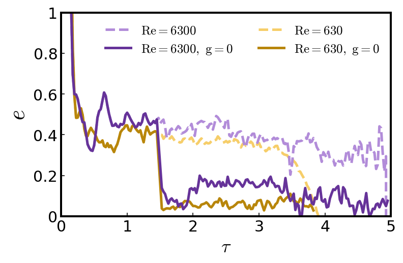
Figure 8: Confirmation of buoyancy-driven entrainment. Plotted is the entrainment efficiency $e$ as a function of time. We directly test the idea of buoyancy-driven entrainment by setting $g=0$ at $\tau=1.5$, sufficiently after the thermals have spun up. The original simulations are dashed lines, and the simulations with where gravity is removed midway through are solid lines. We find in both laminar (yellow) and turbulent (purple) thermals the entrainment efficiency sharply drops off to less than 1/3 of their original values, giving the most direct evidence of the central role of buoyancy in entrainment. The residual entrainment that remains can be attributed to viscous effects, see section 5.1. Deviations occur for the laminar simulations at $\tau>3.5$, because the thermal starts to interact with the top boundary.

In the absence of gravity, the circulation evolves according to

$$\frac{d\Gamma}{dt}\ =\ \int_{\mathcal{S}}\text{Re}^{-1}\nabla^{2}\bm{\omega}\cdot d\bm{A}\ \lesssim 0.$$ (20)

We hypothesize the entrainment seen in Figure 8 is viscous entrainment. It may then be puzzling that the turbulent thermal (with lower viscosity) entrains more than the laminar thermal (with higher viscosity). To understand this, we will now estimate the size of the integrand in Eqn. (20) in both laminar and turbulent cases.

In the laminar thermal, the vorticity is largest on the lengthscale of the vortex radius $R$, so we can estimate $\omega_{\phi}\sim w/R$ and $\nabla\sim R^{-1}$. Then the integrand scales like

$$\quad\quad\text{Re}^{-1}\frac{w}{R^{3}}\quad\quad\text{(laminar)}.$$ (21)

However, in the turbulent case, we see the vorticity is largest on small scales (Figure 1). For turbulent flows, the enstrophy is typically maximum near the viscous scale, $L_{v}\sim R\,\mathrm{Re}^{-3/4}$ (Thorne and Blandford,, 2017). We then estimate $\omega_{\phi}\sim w/L_{v}$ and $\nabla\sim L_{v}^{-1}$, so the integrand scales like

$$\quad\quad\mathrm{Re}^{5/4}\frac{w}{R^{3}}\quad\quad\text{(turbulent)}.$$ (22)

This illustrates that the viscous torques may change the circulation more in turbulent thermals than laminar thermals! This is consistent with the substantially larger entrainment in turbulent thermals than laminar thermals when there is no gravity (Figure 8). Hence, absent gravity, we find there is a small amount of residual entrainment, which is turbulent in origin. These effects are small for buoyant thermals in the presence of gravity.

One subtlety in the argument above is that the integrand in the laminar case is everywhere negative, whereas in the turbulent case, it has both negative and positive contributions, leading to substantial cancellations. We expect that cancellations in the turbulent case will make the net change in circulation due to viscous torques independent of Reynolds number, rather than increasing with Reynolds number. We also note that the slight increase in circulation for the laminar simulation including gravity (Figure 3) is likely due to baroclinic torques, given that the viscous torques should decrease the circulation.

5.2  Conclusion

In this paper, we developed a simple theory for thermals based on the vertical momentum equation (9) and the kinematic constraint (3). This allowed us to derive a complete theory for dry thermals without any additional, empirical constants. We also demonstrated that dry thermals entrain primarily through a buoyancy-driven processes by setting $g=0$ midway through the simulation runs. The entrainment is seen to drop off sharply and the small, residual entrainment that remains can be attributed to viscous dissipation that depends on the Reynolds number of the thermal. This is in contrast to many other explanations of entrainment in convection which rely on a primarily turbulent or stochastic entrainment hypothesis (Romps,, 2010; Escudier and Maxworthy,, 1973; Morton et al.,, 1956).

Our theory also resulted in the explicit expression (17) for the entrainment efficiency, which captures the well-known $F/\Gamma^{2}$ scaling for $e$ and is consistent with parameterizations of gross entrainment as proportional to $B/w^{2}$, as in Tan et al., (2018) and Gregory, (2001). The verification of the $B/w^{2}$ scaling here and the $1/a$ scaling in Lecoanet and Jeevanjee, (2018) might also explain why these scalings outperformed others in the moist convection study of Hernandez-Deckers and Sherwood, (2018).

To truly bridge the gap, however, between our idealized dry thermals and real world cumulus convection, future work should develop a new suite of simulations for moist thermals, perhaps with a simplified model of condensation as in Vallis et al., (2018). The current theory will likely need modification because the assumption of constant integrated buoyancy breaks down in moist thermals, which can generate buoyancy in their center due to latent heat release (Morrison and Peters,, 2018; Romps and Charn,, 2015). As for our Boussinesq approximation, the framework presented in this paper has already been generalized to anelastic and compressible thermals in Anders et al., (2019). They study thermals in the context of solar convection, and the excellent agreement between theory and simulation in their more general paradigm suggests that our framework might also be amenable to moist thermals. A simple model for the moist case would provide a foundation on which a thorough understanding of cumulus convection may be built, bridging the gap between simulation and theory in climate and atmospheric modeling (Jeevanjee et al.,, 2017; Held,, 2005).

References

- Akhmetov, (2009) Akhmetov, D. G. (2009). Vortex rings. Springer Berlin Heidelberg, Berlin, Heidelberg.
- Anders et al., (2019) Anders, E., Lecoanet, D., and Brown, B. (2019). Entropy Rain: Dilution of Thermals in Stratified Domains. arxiv preprint https://arxiv.org/abs/1906.02342.
- Asai and Kasahara, (1967) Asai, T. and Kasahara, A. (1967). A Theoretical Study of the Compensating Downward Motions Associated with Cumulus Clouds. Journal of the Atmospheric Sciences, 24(5):487–496.
- Baker et al., (1984) Baker, M. B., Breidenthal, R. E., Choularton, T. W., and Latham, J. (1984). The Effects of Turbulent Mixing in Clouds. Journal of the Atmospheric Sciences, 41(6):299–304.
- Batchelor, (2000) Batchelor, G. K. (2000). An Introduction to Fluid Dynamics. Cambridge University Press.
- Bond and Johari, (2010) Bond, D. and Johari, H. (2010). Impact of buoyancy on vortex ring development in the near field. Experiments in Fluids, 48(5):737–745.
- Burns et al., (2019) Burns, K. J., Vasil, G. M., Oishi, J. S., Lecoanet, D., and Brown, B. P. (2019). Dedalus: A Flexible Framework for Numerical Simulations with Spectral Methods. arXiv e-prints, page arXiv:1905.10388.
- Craig and Dörnbrack, (2008) Craig, G. C. and Dörnbrack, A. (2008). Entrainment in Cumulus Clouds: What Resolution is Cloud-Resolving? Journal of the Atmospheric Sciences, 65(12):3978–3988.
- de Rooy et al., (2013) de Rooy, W. C., Bechtold, P., Fröhlich, K., Hohenegger, C., Jonker, H., Mironov, D., Pier Siebesma, A., Teixeira, J., and Yano, J.-I. (2013). Entrainment and detrainment in cumulus convection: an overview. Quarterly Journal of the Royal Meteorological Society, 139(670):1–19.
- de Rooy and Siebesma, (2010) de Rooy, W. C. and Siebesma, A. P. (2010). Analytical expressions for entrainment and detrainment in cumulus convection. Quarterly Journal of the Royal Meteorological Society, 136(650):1216–1227.
- Escudier and Maxworthy, (1973) Escudier, M. P. and Maxworthy, T. (1973). On the motion of turbulent thermals. Journal of Fluid Mechanics, 61(3):541–552.
- Ferrier and Houze, (1989) Ferrier, B. S. and Houze, R. A. (1989). One-Dimensional Time-Dependent Modeling of GATE Cumulonimbus Convection. Journal of the Atmospheric Sciences, 46(3):330–352.
- Fohl, (1967) Fohl, T. (1967). Turbulent Effects in the Formation of Buoyant Vortex Rings. Journal of Applied Physics, 38(10):4097–4098.
- Gregory, (2001) Gregory, D. (2001). Estimation of entrainment rate in simple models of convective clouds. Quarterly Journal of the Royal Meteorological Society, 127(571):53–72.
- Held, (2005) Held, I. M. (2005). The gap between simulation and understanding in climate modeling. Bulletin of the American Meteorological Society, 86(11):1609–1614.
- Hernandez-Deckers and Sherwood, (2018) Hernandez-Deckers, D. and Sherwood, S. C. (2018). On the Role of Entrainment in the Fate of Cumulus Thermals. Journal of the Atmospheric Sciences, 75(11):3911–3924.
- Houghton and Cramer, (1951) Houghton, H. G. and Cramer, H. E. (1951). A Theory of entrainment in convective currents. Journal of Meteorology, 8(2):95–102.
- Jeevanjee et al., (2017) Jeevanjee, N., Hassanzadeh, P., Hill, S., and Sheshadri, A. (2017). A perspective on climate model hierarchies. Journal of Advances in Modeling Earth Systems, 9(4):1760–1771.
- Johari, (1992) Johari, H. (1992). Mixing in Thermals with and without Buoyancy Reversal.
- Klocke et al., (2011) Klocke, D., Pincus, R., and Quaas, J. (2011). On constraining estimates of climate sensitivity with present-day observations through model weighting. Journal of Climate, 24(23):6092–6099.
- Lai et al., (2015) Lai, A. C. H., Zhao, B., Law, A. W.-K., and Adams, E. E. (2015). A numerical and analytical study of the effect of aspect ratio on the behavior of a round thermal. Environmental Fluid Mechanics, 15(1):85–108.
- Lamb and Caflisch, (1993) Lamb, H. and Caflisch, R. (1993). Hydrodynamics. Cambridge Mathematical Library. Cambridge University Press.
- Lecoanet and Jeevanjee, (2018) Lecoanet, D. and Jeevanjee, N. (2018). Entrainment in Resolved, Turbulent Dry Thermals. arxiv preprint, http://arxiv.org/abs/1804.09326.
- Levine, (1959) Levine, J. (1959). Spherical Vortex Theory of Bubble-like Motion in Cumulus Clouds. Journal of Meteorology, 16:653–662.
- Morrison, (2017) Morrison, H. (2017). An Analytic Description of the Structure and Evolution of Growing Deep Cumulus Updrafts. Journal of the Atmospheric Sciences, 74(3):809–834.
- Morrison and Peters, (2018) Morrison, H. and Peters, J. M. (2018). Theoretical Expressions for the Ascent Rate of Moist Deep Convective Thermals. Journal of the Atmospheric Sciences, 75(5):1699–1719.
- Morton et al., (1956) Morton, B. R., Taylor, G., and Turner, J. S. (1956). Turbulent Gravitational Convection from Maintained and Instantaneous Sources. Proceedings of the Royal Society A: Mathematical, Physical and Engineering Sciences, 234(1196):1–23.
- Romps, (2010) Romps, D. M. (2010). A Direct Measure of Entrainment. Journal of the Atmospheric Sciences, 67(6):1908–1927.
- Romps and Charn, (2015) Romps, D. M. and Charn, A. B. (2015). Sticky Thermals: Evidence for a Dominant Balance between Buoyancy and Drag in Cloud Updrafts. Journal of the Atmospheric Sciences, 72(8):2890–2901.
- Romps and Kuang, (2010) Romps, D. M. and Kuang, Z. (2010). Nature versus Nurture in Shallow Convection. Journal of the Atmospheric Sciences, 67(5):1655–1666.
- Sànchez et al., (1989) Sànchez, O., Raymond, D. J., Libersky, L., and Petschek, A. G. (1989). The Development of Thermals from Rest. Journal of Atmospheric Sciences, 46:2280–2292.
- Scorer, (1957) Scorer, R. S. (1957). Experiments on convection of isolated masses of buoyant fluid. Journal of Fluid Mechanics, 2:583–594.
- Shariff and Leonard, (1992) Shariff, K. and Leonard, A. (1992). Vortex Rings. Annual Review of Fluid Mechanics, 24(1):235–279.
- Sherwood et al., (2013) Sherwood, S. C., Hernández-Deckers, D., Colin, M., and Robinson, F. (2013). Slippery Thermals and the Cumulus Entrainment Paradox*. Journal of the Atmospheric Sciences, 70(8):2426–2442.
- Shivamoggi, (2010) Shivamoggi, B. K. (2010). Hydrodynamic Impulse in a Compressible Fluid. eprint arXiv:0910.3223, pages 1–10.
- Simpson, (1983) Simpson, J. (1983). Cumulus Clouds: Interactions Between Laboratory Experiments and Observations as Foundations for Models. In Mesoscale Meteorology — Theories, Observations and Models, pages 399–412. Springer Netherlands, Dordrecht.
- Simpson and Wiggert, (1969) Simpson, J. and Wiggert, V. (1969). Models of Precipitating Cumulus Towers. Monthly Weather Review, 97(7):471–489.
- Tan et al., (2018) Tan, Z., Kaul, C. M., Pressel, K. G., Cohen, Y., Schneider, T., and Teixeira, J. (2018). An Extended Eddy-Diffusivity Mass-Flux Scheme for Unified Representation of Subgrid-Scale Turbulence and Convection. Journal of Advances in Modeling Earth Systems, 10(3):770–800.
- Tarshish et al., (2018) Tarshish, N., Jeevanjee, N., and Lecoanet, D. (2018). Buoyant Motion of a Turbulent Thermal. Journal of the Atmospheric Sciences, in press:JAS–D–17–0371.1.
- Thorne and Blandford, (2017) Thorne, K. S. and Blandford, R. D. (2017). Modern Classical Physics: Optics, Fluids, Plasmas, Elasticity, Relativity, and Statistical Physics. Princeton University Press.
- Turner, (1957) Turner, J. S. (1957). Buoyant Vortex Rings. Proceedings of the Royal Society A: Mathematical, Physical and Engineering Sciences, 239(1216):61–75.
- Turner, (1962) Turner, J. S. (1962). The ‘starting plume’ in neutral surroundings. Journal of Fluid Mechanics, 13(3):356–368.
- Turner, (1964) Turner, J. S. (1964). The dynamics of spheroidal masses of buoyant fluid. Journal of Fluid Mechanics, 19(4):481–490.
- Turner, (1986) Turner, J. S. (1986). Turbulent entrainment: the development of the entrainment assumption, and its application to geophysical flows. Journal of Fluid Mechanics, 173:431–471.
- Turner et al., (1973) Turner, J. S., Turner, J. S., and Press, C. U. (1973). Buoyancy Effects in Fluids. Cambridge Bible Commentary: New English Bible. Cambridge University Press.
- Vallis et al., (2018) Vallis, G. K., Parker, D. J., and Tobias, S. M. (2018). A Simple System for Moist Convection: the Rainy-Benard Model. Journal of Fluid Mechanics, 862:162–199.
- Yano, (2014) Yano, J. I. (2014). Basic convective element: Bubble or plume? A historical review. Atmospheric Chemistry and Physics, 14(13):7019–7030.
- Zhao et al., (2013) Zhao, B., Law, A. W. K., Lai, A. C. H., and Adams, E. E. (2013). On the internal vorticity and density structures of miscible thermals. Journal of Fluid Mechanics, 722:1–12.
- Zhao, (2014) Zhao, M. (2014). An investigation of the connections among convection, clouds, and climate sensitivity in a global climate model. Journal of Climate, 27(5):1845–1862.