PNDME Collaboration
Nucleon Electromagnetic Form Factors in the Continuum Limit from 2+1+1-flavor Lattice QCD
Abstract
We present results for the isovector electromagnetic form factors of the nucleon using eleven ensembles of gauge configurations generated by the MILC collaboration using the highly improved staggered quark (HISQ) action with 2+1+1 dynamical flavors. These ensembles span four lattice spacings 0.06, 0.09, 0.12 and 0.15 fm and three values of the light-quark masses corresponding to the pion masses and . High-statistics estimates using the truncated solver method method allow us to quantify various systematic uncertainties and perform a simultaneous extrapolation in the lattice spacing, lattice volume and light-quark masses. We analyze the dependence of the form factors calculated over the range GeV2 using both the model independent -expansion and the dipole ansatz. Our final estimates, using the -expansion fit, for the isovector root-mean-square radius of nucleon are , and Bohr magneton. The first error is the combined uncertainty from the leading-order analysis, and the second is an estimate of the additional uncertainty due to using the leading order chiral-continuum-finite-volume fits. The estimates from the dipole ansatz, , and Bohr magneton, are consistent with those from the -expansion but with smaller errors. Our analysis highlights three points. First, all our data for form factors from the eleven ensembles and existing lattice data on, or close to, physical mass ensembles from other collaborations collapses more clearly onto a single curve when plotted versus as compared to with the scale set by quantities other than . The difference between these two ways of analyzing the data is indicative of discretization errors, some of which presumably cancel when the data are plotted versus . Second, the size of the remaining deviation of this common curve from the Kelly curve is small and can be accounted for by statistical and possible systematic uncertainties. Third, to improve lattice estimates for , and , high statistics data for GeV2 are needed.
pacs:
11.15.Ha, 12.38.GcI Introduction
Experiments studying electron scattering off protons and neutrons have a long history of providing an understanding of the structure of nucleons Perdrisat et al. (2007); Punjabi et al. (2005). Quantitative understanding of the distribution of charge is described by the electric and magnetic form factors, and Bernauer et al. (2014). Quantities of phenomenological interest obtained from the slope of the form factors at space-like four momentum transfer squared are the electric and magnetic charge radii of the nucleons. At present there is a 6 discrepancy between the electric charge radius of the proton obtained from electronic energy levels combined with electron scattering data Mohr et al. (2016) versus that from the Lamb shift in muonic hydrogen Antognini et al. (2013, 2016). A second issue that needs resolution is the behavior of the ratio at GeV2 Ye et al. (2018), and whether this ratio crosses zero at about GeV2 as indicated by experiments at JLab Gayou et al. (2002); Electro-Magnetic Form Factor collaboration, Jefferson Lab() (EMFF). In this work, we focus on determining the electromagnetic form factors in the range GeV2 and extracting the charge radii from them.
The electric and magnetic form factors, and , of the nucleon can be calculated directly from large scale simulations of lattice QCD. In recent years, advances in algorithms and computing power have allowed the community to push the calculations towards physical masses for the light and quarks, and on lattice spacings that are small enough that discretization effects are expected to be at the few percent level Bhattacharya et al. (2014); Green et al. (2014); Capitani et al. (2015); Alexandrou et al. (2017a). In this paper we present results from thirteen calculations on eleven ensembles that cover a range of lattice spacings ( fm), pion masses ( MeV) and lattice volumes (). These ensembles were generated using -flavors of highly improved staggered quarks (HISQ) Follana et al. (2007) by the MILC collaboration Bazavov et al. (2013). This suite of calculations allows us to understand and assess various sources of systematic errors. The analysis is carried out using both the dipole ansatz and the -expansion, which give consistent estimates for the isovector mean-square charge radii and and the magnetic moment .
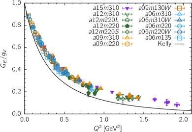
Our final results for the isovector mean-square charge radii and (also for Dirac, , and Pauli, , radii) defined in Eqs. (10), (11) and (12), and for the magnetic moment are given in Tab. 9. We also present a comparison with other lattice data obtained close to the physical pion mass and with the Kelly parameterization of the experimental data Kelly (2004) in Fig. 22. Our estimates for , and are about 17%, 19%, and 16% smaller than the phenomenological values given in Eq. (30) and the precise experimental value in Eq. (9). Throughout this paper, we have paid attention to the size of possible statistical and systematic errors, and find that a linear combination of these is large enough to explain the deviations.
We analyze the world data for and in Sec. VII and find that data from all 13 of our calculations and those from other collaborations done at or near the physical pion mass fall roughly onto a single curve when plotted versus versus or . However, there is a noticeable shift between the two curves when compared to the Kelly fit. The difference between the two ways of analyzing the data is a discretization artifact: specifically, it is a consequence of the difference in values of the lattice scale obtained from different observables. The size of the difference again indicates that the present underestimate of , and should not be considered significant. Our overall conclusion is that to significantly reduce the systematics and improve the precision with which these observables can be extracted will require high statistics data at smaller values of the lattice spacing and of GeV2.
We stress that the long-term goal of lattice QCD is to directly predict the form factors and not to reproduce the Kelly curve, a parameterization of the experimental data. Throughout this paper, we use the Kelly curve to provide a reference point for comparison, and for discussing systematics and trends in the lattice data. We do not show an error band on the Kelly curve as it is negligible on the scale of the errors in the lattice data.
This paper is organized as follows. In Sec. II, we review the theory, computational approach and the status of the experimental and phenomenological results. In Sec. III, we describe the salient features of the calculation. The fits used to isolate excited-state contamination (ESC) and extract the form factors are described in Sec. IV. Fits to quantify the behavior of the form factors are discussed in Sec. V, and the extraction of our final results for the isovector mean-square charge radii, and , and the anomalous magnetic moment are presented in Sec. VI. Comparisons with form factors extracted from experiments and with previous lattice QCD calculations are made in Sec. VII. We end with conclusions in Sec. VIII. Some further details of the calculations are given in four Appendices: lattice parameters in Appendix A, analysis of nucleon mass in Appendix B, ESC in Appendix C, and a review of the experimental data for the form factors in Appendix D.
II Electromagnetic Form Factors of the Nucleon
The Dirac, , and Pauli, , form factors are extracted from the matrix elements of the electromagnetic current within the nucleon state through the relation
| (1) |
where is the momentum transfer. The discrete lattice momenta are given by with the entries of the vector taking on integer values, . The spacing between the momenta is controlled by the spatial lattice size, . The normalization used for the nucleon spinors in Euclidean space is
| (2) |
and in Eq. (1), the electromagnetic current is
| (3) |
In the isospin symmetric limit, the difference of its matrix elements between a proton and a neutron state are related to the isovector form factors of the proton by the relation
| (4) |
The quantity we calculate on the lattice is the left hand side of Eq. (4), i.e., the isovector form factors of the proton. Throughout this paper, the term isovector form factors of the proton and the form factors refer to the same quantities as defined in Eq. (4). These will henceforth be analyzed in terms of the space-like 4-momentum squared, .
Another common set of definitions of the electromagnetic form factors, widely used in the analysis of experimental data, are the Sachs electric, , and magnetic, , form factors that are related to the Dirac and Pauli form factors as
| (5) | ||||
| (6) |
From these, the vector charge is given by
| (7) |
and the difference between the magnetic moment of the proton and the neutron by
| (8) |
The anomalous magnetic moments of the proton and the neutron, in units of the Bohr magneton, are known very precisely Patrignani et al. (2016):
| (9) |
The electric and magnetic size of the nucleon are defined as the slope of the form factors with respect to at Miller (2019):
| (10) |
The form factors are normalized by their values at : and . This definition makes them independent of the renormalization constant, , of the lattice vector current, and improves the signal because some of the systematics cancel in the ratios. Therefore, in this work, we will use Eq. (10) when calculating and . Note that as the electric charge is conserved. A second independent estimate of , obtained using nonperturbative lattice calculations in the RI-sMOM scheme, is given in Ref. Gupta et al. (2018), where the difference between the two estimates was shown to be .
One similarly defines the isovector Dirac and Pauli mean-square radii as
| (11) |
These are related to , and as
| (12) |
Our analysis of the lattice data is carried out in terms of and . Results for and are also given in Table 9 in Sec. VI, where we extract and .
The electric root-mean-square charge radius of the proton has been measured in three ways: (i) laser spectroscopy of the Lamb shift in muonic hydrogen Antognini et al. (2013, 2016); Krauth et al. (2017), (ii) continuous-wave laser spectroscopy of hydrogen Pohl et al. (2017), and (iii) elastic scattering of electrons off protons Sick and Trautmann (2014, 2017). Results using electrons, i.e., the latter two ways, are included in the CODATA-2014 world average Tanabashi et al. (2018); Mohr et al. (2016):
| (13) |
and the third result is from muonic hydrogen. The large difference between the CODATA-2014 and muonic-hydrogen values was termed the “proton radius puzzle”. The new CODATA-2018 value CODATA-2018 resolves the puzzle in favor of the muonic-hydrogen result. The magnetic radius of the proton extracted from experiments using electrons is Tanabashi et al. (2018); Mohr et al. (2016)
| (14) |
Values for the isovector charge radii, extracted from the experimental data and used to compare lattice data against, are given in Eq. (30) in Appendix D.
To reduce the uncertainty in results from electron scattering experiments, which have been done down to GeV2, new experiments to constrain the low behavior have been initiated Weber et al. (2016); Gasparian (2017). Similarly, for lattice QCD calculations to help resolve the puzzle, we need to calculate the form factors to GeV2 to extract with better than 1% accuracy.
A challenge to the direct extraction of from the lattice data is that the value of the smallest momenta, , is large in typical lattice simulations. In our calculations, it is MeV, and the range of values, given in Table 1, are between 2–10 . It is, therefore, traditional to fit the data for the to an ansatz, and then use the fit to evaluate the derivative given in Eq. (10). Both, using an ansatz and estimating its parameters from fits to data with MeV introduces systematic uncertainties when evaluating the derivative at . We estimate the dependence of on the choice of the ansatz by comparing results for each ensemble obtained using two different fits, the dipole model and the -expansion.
Two alternate approaches are, one, to calculate the form factors at fixed and extrapolate these to the continuum limit first and then fit the behavior. Unfortunately, the values of are different on each ensemble. Second, combine the dipole or the -expansion parameterization of the behavior with the chiral-continuum-finite volume (CCFV) ansatz for one overall fit. This combined fit is discussed in Sec. VI.2. The central analysis presented here consists of first fitting the data versus using the dipole model and the -expansion to extract and on each ensemble and then get the physical results from a CCFV fit in , and that addresses the associated systematics.
It is important to note that both the electron scattering experiments and lattice QCD calculations suffer from paucity of data close to that impacts the extraction of the charge radii. However, there is a large range, GeV2 over which accurate experimental data exist. Thus, more than just extracting the charge radii, our goal is to directly compare the lattice and the experimental data over this range of as discussed in Sec. V.
An ansatz that is commonly used to fit the experimental data is the dipole. It arises if one assumes an exponentially falling charge distribution. The resulting form factor is characterized by a single parameter, the mass ,
| (15) |
and normalized to at . It goes as in the limit in accord with perturbation theory Lepage and Brodsky (1980).
The second ansatz is a model-independent parameterization called the -expansion Hill and Paz (2010); Bhattacharya et al. (2011):
| (16) |
where the are fit parameters and is defined as
| (17) |
with denoting the nearest singularity in . In terms of , the domain of analyticity of is mapped into the unit circle with the branch cut at Bhattacharya et al. (2011). We analyzed the data with and GeV2 for the MeV ensembles. By choosing the value of the constant to lie in the middle of the range of at which we have data, one reduces . By reducing the value of we hope to improve the stability of the estimates, with improvement judged by comparing result from different truncations of the series. In practice, for our data set, we find that the quality of the fits and the results are insensitive to the choice of . The final results for the charge radii and magnetic moment are obtained from fits using .
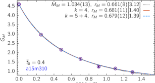
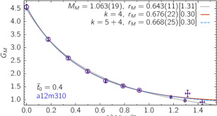
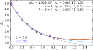
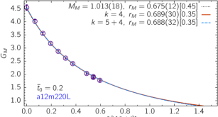
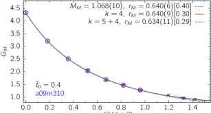
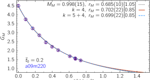
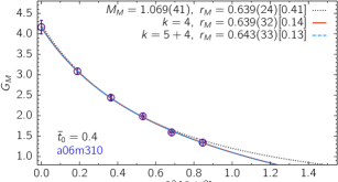
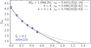
The values of for the thirteen calculations are given in Table 1. Note that in four cases the number of nonzero values are only five. The data for and versus with are shown in Fig. 8. As discussed in Sec. V.2, we restrict our fits to GeV2 because the reliability of some of the higher data is questionable.
To implement the perturbative behavior as Lepage and Brodsky (1980) in the -expansion requires for . These constraints can be incorporated into the z-expansion as four sum rules Lee et al. (2015)
| (18) |
For it reduces to . A priori, using these sum rules ensures that the are not only bounded but must also decrease at large Lee et al. (2015).
A key issue in the -expansion analysis is the value of required to obtain results with a certain precision. The analysis of the experimental data carried out in Appendix D shows that results stabilize for with and without sum rules. For the lattice data, the choice has to take into account the number of values of at which data have been generated to not over-parameterize the fit. For our data and fits without priors, the fluctuate and the higher order coefficients () are ill determined due to the over-parameterization of the fits. To avoid the resulting large fluctuations in , we put a bound on them as suggested in Lee et al. (2015). For and , we constrain for all by using Gaussian priors with central value zero and width five. With this constraint, results for , and do not change significantly for and stabilize for as shown in Fig. 9. The convergence of estimates from fits with sum rules is slower and occurs for as also shown in Fig. 9. We, therefore, use the fits with and without sum rules for our final results as they converge faster. Results with sum rules, which converge for , are used only as consistency checks. Since , and are best extracted from data at small , the sum rule constraints imposed to guarantee the large behavior are not essential for their determination.
Overall, the fits to are more stable than those to . The main reason is the extra data point at which pins down the sign of the slope of at small . Using a value for , derived from the ratio as discussed in Sec. IV.2, greatly improved the stability of fits to .
III Lattice Methodology
The parameters of the thirteen calculations done on eleven HISQ ensembles are the same as used in Ref. Gupta et al. (2018) for the calculation of isovector charges. To keep the paper self-contained, the lattice parameters of the calculations and the number of measurements made are summarized in Table 12 in the appendix A. The parameters used to generate the Wilson-clover quark propagators using the multigrid algorithm Babich et al. (2010) are also given in Table. 13. We remind the reader that two ensembles, and , have been analyzed twice with different smearing parameters giving a total of 13 calculations. Also, compared to Refs. Bhattacharya et al. (2016); Gupta et al. (2017), six ensembles (, , , , and ) have been simulated afresh with randomly chosen source points on each configuration to increase their statistical independence, and data at a larger number of momenta have been accumulated.
To increase the statistics cost-effectively, we used the truncated solver with bias correction method Bali et al. (2010); Blum et al. (2013). We also used the coherent source method to construct sequential propagators from the sink time slice, at which a zero-momentum nucleon state is inserted Bratt et al. (2010); Yoon et al. (2016).
The details of our strategy for the calculations and the analysis have been published in earlier works Bhattacharya et al. (2016); Gupta et al. (2017, 2018). Here we provide a brief summary of the points relevant to the calculation of the electric and magnetic form factors:
-
•
All errors are determined using a single elimination jackknife method over configurations, i.e., we first construct the bias corrected average for each configuration and then carry out the fits to the two- and three-point functions within the same jackknife procedure over these configuration averages.
-
•
To control excited-state contamination, we use the same toolkit as in Ref. Gupta et al. (2018). The 2-point functions are fit keeping four states in the spectral decomposition. The amplitudes and the masses obtained from these fits are input into the analysis of three-point functions. The results for the masses are given in Table 14 in Appendix B.
- •
-
•
The insertion of the vector current at definite momenta is carried out on each time slice between the source and the sink, and for each value of . These data for the three-point functions, , at a large number of values of and are fit using three states in the spectral decomposition:
(19) where the source point is translated to , the operator is inserted at time , and the nucleon state is annihilated at the sink time slice , which numerically is also the source-sink separation. In this relation, the numbers refer to the state , a state with superscript ′ denotes that it could have nonzero momentum , and the momentum at the sink is fixed to zero.
-
•
With our data, the term could not be resolved. So, in all the fits we set the contribution of the term with equal to zero, and call these -state fits.
-
•
In the case of data, the data are analyzed using -state fits, while the data are fit using two states because the -state fits for are unstable. Having stated this caveat, we will, for brevity, use the label -state to describe the excited-state fits to all data, even those for this ensemble.
-
•
The values of at which the form factors are calculated are collected in Table 1. These are obtained using the nucleon ground-state energy extracted using 4-state fits to the 2-point functions.
-
•
To extract the desired matrix element using Eq. (19), the masses , energies , and the amplitudes and are taken from the fit to the two-point function within one overall jackknife procedure. This assumes that the ordering of the coupling to the excited states is the same as in two-point functions. To improve the signal, the amplitude with which the nucleon interpolating operator at the source time slice couples to the ground state with energy and momentum should be large while the coupling to excited states should be small. We find that for the smearing parameters given in Table. 13, the signal in all the ten momentum channels analyzed is good.
-
•
Off diagonal terms with nonzero momentum transfer such as are related to by a combination of Lorentz boost, parity and hermitian transformation provided the tower of states and the coupling to them are the same on either side of the operator. In our calculation, the nucleon operator used is
(20) with color indices , charge conjugation matrix , and and denoting the two different flavors of light Dirac quarks. The quark propagator is smeared both at the source and the sink using a gauge invariant Gaussian smearing procedure Güsken et al. (1989) described in Appendix A. The nonrelativistic projection , inserted to improve the signal Bhattacharya et al. (2015, 2016); Yoon et al. (2017), as well as the smearing of the quark fields, breaks Lorentz covariance. Also, the sink is explicitly constructed to have . We, therefore, treat all such pair of matrix elements as independent free parameters in the fits.
-
•
The data for 3-point functions at nonzero momentum transfer are not symmetric about the midpoint, , between the source and the sink. Nevertheless, in the simultaneous 3-state fit to the data with multiple source-sink separations and intermediate times , we skip the same points adjacent to the source and the sink for every to remove points with the largest ESC. Two considerations motivated this choice: (i) the time slice of the onset of the plateau in the nucleon effective mass plot is roughly independent of the momentum as shown in Refs. Gupta et al. (2017, 2018), and (ii) because we choose the values of to be as small as possible based on the stability of the covariance matrix used in the fits. The values of used here are the same as in Ref. Gupta et al. (2018).
-
•
The vector current in the continuum theory is conserved, however the local vector current used in our lattice calculations is not. The renormalization constant for this current has been determined in two ways: (i) nonperturbatively in the RI-sMOM scheme and then converted to using perturbation theory and (ii) measured directly from the matrix element of at , i.e., . The two sets of values are compared in Ref. Gupta et al. (2018) and differ by up to 3%. This size of difference is not unreasonable in our clover-on-HISQ formulation which has discretization effects starting at . Here, we implement method (ii) by forming ratios , in which some of the systematics cancel. The discretization errors in , and are addressed by the continuum extrapolation, a part of the CCFV fit.
The key input, other than statistical precision of the 3-point data, that impacts the stability of the n-state fits to control ESC and obtain the ground state matrix elements is the energy of the first excited state since the terms with and give the dominant contribution. Once the ground-state matrix elements have been determined, the procedure for obtaining the form factors from them is described in the next section.
| 0.2519(5) | 0.1765(5) | 0.0670(1) | 0.1047(4) | 0.1747(15) | 0.1834(3) | 0.0861(2) | |
| 0.4831(14) | 0.3415(13) | 0.1318(2) | 0.2060(15) | 0.3386(35) | 0.3558(12) | 0.1685(4) | |
| 0.7034(25) | 0.4982(24) | 0.1947(4) | 0.3012(20) | 0.4905(61) | 0.5198(43) | 0.2479(8) | |
| 0.9111(60) | 0.6459(35) | 0.2565(8) | 0.3909(25) | 0.6358(87) | 0.6735(44) | 0.3244(14) | |
| 1.1020(67) | 0.7871(42) | 0.3159(10) | 0.4824(37) | 0.774(10) | 0.8186(79) | 0.3983(18) | |
| 1.2971(91) | 0.9202(52) | 0.3740(13) | 0.5678(47) | 0.910(13) | 0.9610(127) | 0.4703(23) | |
| 1.6372(215) | 1.178(9) | 0.4872(21) | 0.7321(81) | 1.178(23) | 1.1974(92) | 0.6077(37) | |
| 1.8026(222) | 1.293(10) | 0.5413(25) | 0.8077(103) | 1.307(25) | 1.3229(131) | 0.6743(44) | |
| 1.7896(289) | 1.315(19) | 0.5412(28) | 0.8064(118) | 1.238(33) | 1.3248(168) | 0.6713(46) | |
| 1.9171(314) | 1.435(18) | 0.5950(32) | 0.8845(124) | 1.358(36) | 1.4210(144) | 0.7357(51) | |
| 0.0492(2) | 0.1888(13) | 0.1899(6) | 0.1101(3) | 0.1093(3) | 0.0513(2) | ||
| 0.0974(5) | 0.3648(33) | 0.3653(15) | 0.2159(11) | 0.2132(9) | 0.1014(6) | ||
| 0.1450(9) | 0.5322(70) | 0.5277(29) | 0.3175(24) | 0.3130(19) | 0.1510(12) | ||
| 0.1913(15) | 0.6828(99) | 0.6895(48) | 0.4142(46) | 0.4120(55) | 0.1975(15) | ||
| 0.2373(18) | 0.8457(118) | 0.8402(65) | 0.5087(57) | 0.5045(61) | 0.2459(22) | ||
| 0.2824(23) | 0.2941(32) | ||||||
| 0.3704(33) | 0.3866(47) | ||||||
| 0.4108(41) | 0.4323(51) | ||||||
| 0.4067(48) | 0.4259(60) | ||||||
| 0.4490(50) | 0.4703(65) |
| 1.069(4) | 1.061(8) | 1.067(4) | 1.071(9) | 1.081(18) | 1.045(3) | 1.049(4) | |
| 0.650(4) | 0.728(8) | 0.908(12) | 0.840(11) | 0.706(17) | 0.735(4) | 0.859(5) | |
| 0.440(4) | 0.536(9) | 0.789(12) | 0.666(23) | 0.513(17) | 0.549(6) | 0.718(7) | |
| 0.321(4) | 0.407(10) | 0.694(11) | 0.553(16) | 0.402(20) | 0.423(12) | 0.614(8) | |
| 0.261(8) | 0.332(11) | 0.618(12) | 0.469(15) | 0.324(20) | 0.348(7) | 0.538(9) | |
| 0.212(5) | 0.279(8) | 0.553(10) | 0.396(17) | 0.279(18) | 0.285(9) | 0.472(8) | |
| 0.167(6) | 0.239(9) | 0.499(9) | 0.349(15) | 0.234(17) | 0.240(9) | 0.417(8) | |
| 0.140(15) | 0.176(15) | 0.413(8) | 0.280(19) | 0.156(24) | 0.186(4) | 0.338(8) | |
| 0.114(12) | 0.161(12) | 0.380(7) | 0.260(16) | 0.155(21) | 0.162(4) | 0.307(7) | |
| 0.110(30) | 0.157(35) | 0.387(8) | 0.203(32) | 0.148(42) | 0.177(8) | 0.315(9) | |
| 0.088(20) | 0.155(24) | 0.357(7) | 0.200(23) | 0.154(27) | 0.153(5) | 0.290(7) | |
| 1.052(6) | 1.043(6) | 1.035(11) | 1.050(7) | 1.039(9) | 1.042(10) | ||
| 0.937(6) | 0.700(16) | 0.711(9) | 0.822(8) | 0.811(9) | 0.919(10) | ||
| 0.836(6) | 0.502(21) | 0.521(8) | 0.670(10) | 0.654(11) | 0.814(13) | ||
| 0.756(6) | 0.373(24) | 0.395(9) | 0.552(14) | 0.536(14) | 0.716(18) | ||
| 0.680(8) | 0.306(24) | 0.318(13) | 0.465(17) | 0.440(26) | 0.664(15) | ||
| 0.624(8) | 0.232(23) | 0.260(11) | 0.398(17) | 0.384(20) | 0.588(18) | ||
| 0.571(8) | 0.528(20) | ||||||
| 0.497(9) | 0.433(21) | ||||||
| 0.455(9) | 0.399(19) | ||||||
| 0.439(15) | 0.422(21) | ||||||
| 0.418(12) | 0.380(20) |
| 0.610(15) | 0.818(50) | 0.871(30) | 0.761(61) | 0.774(59) | 0.699(17) | 0.814(30) | |
| 0.435(10) | 0.592(32) | 0.786(27) | 0.634(69) | 0.564(38) | 0.536(16) | 0.694(26) | |
| 0.336(10) | 0.448(27) | 0.711(28) | 0.575(42) | 0.439(36) | 0.413(29) | 0.619(25) | |
| 0.262(21) | 0.410(32) | 0.654(28) | 0.527(42) | 0.432(39) | 0.358(14) | 0.551(27) | |
| 0.205(13) | 0.340(24) | 0.585(24) | 0.429(36) | 0.316(32) | 0.296(17) | 0.479(22) | |
| 0.158(14) | 0.284(24) | 0.543(23) | 0.334(37) | 0.249(37) | 0.255(14) | 0.422(21) | |
| 0.135(10) | 0.193(27) | 0.464(22) | 0.284(37) | 0.181(33) | 0.206(8) | 0.362(18) | |
| 0.103(25) | 0.166(30) | 0.429(21) | 0.250(43) | 0.161(45) | 0.182(8) | 0.308(19) | |
| 0.139(43) | 0.188(66) | 0.445(25) | 0.249(59) | 0.202(59) | 0.195(15) | 0.342(17) | |
| 0.083(58) | 0.178(76) | 0.405(25) | 0.150(74) | 0.220(92) | 0.172(17) | 0.330(25) | |
| 0.871(43) | 0.733(59) | 0.641(44) | 0.718(46) | 0.778(65) | 0.793(65) | ||
| 0.791(34) | 0.515(49) | 0.500(29) | 0.600(40) | 0.660(49) | 0.688(57) | ||
| 0.710(31) | 0.367(64) | 0.400(30) | 0.534(43) | 0.553(51) | 0.626(64) | ||
| 0.679(31) | 0.390(48) | 0.270(42) | 0.444(53) | 0.413(88) | 0.643(49) | ||
| 0.625(27) | 0.219(34) | 0.229(37) | 0.420(42) | 0.366(67) | 0.529(52) | ||
| 0.582(27) | 0.446(55) | ||||||
| 0.494(26) | 0.399(54) | ||||||
| 0.461(26) | 0.354(54) | ||||||
| 0.467(38) | 0.367(60) | ||||||
| 0.435(33) | 0.311(58) |
| 4.596(61) | 4.553(107) | 4.538(107) | 4.465(144) | 4.597(217) | 4.324(32) | 4.505(76) | |
| 2.968(29) | 3.318(51) | 4.018(61) | 3.657(90) | 3.139(85) | 3.207(19) | 3.749(51) | |
| 2.160(32) | 2.597(43) | 3.557(41) | 3.082(76) | 2.352(75) | 2.513(24) | 3.249(40) | |
| 1.665(26) | 2.092(46) | 3.172(32) | 2.660(68) | 1.940(82) | 2.041(42) | 2.863(36) | |
| 1.255(45) | 1.728(59) | 2.874(31) | 2.251(75) | 1.566(98) | 1.684(32) | 2.468(46) | |
| 1.155(28) | 1.532(41) | 2.615(30) | 2.009(66) | 1.389(74) | 1.471(35) | 2.225(38) | |
| 0.959(31) | 1.363(31) | 2.407(29) | 1.818(67) | 1.257(68) | 1.283(41) | 2.034(36) | |
| 0.817(50) | 1.106(54) | 2.032(37) | 1.643(76) | 1.164(92) | 1.074(18) | 1.698(35) | |
| 0.760(47) | 0.969(55) | 1.913(32) | 1.448(75) | 0.963(82) | 0.982(19) | 1.554(36) | |
| 0.717(102) | 1.241(128) | 1.883(41) | 1.422(88) | 0.851(136) | 0.947(35) | 1.585(44) | |
| 0.734(33) | 0.911(104) | 1.771(41) | 1.424(89) | 0.917(111) | 0.913(49) | 1.467(36) | |
| 4.297(82) | 4.163(168) | 4.303(134) | 4.138(102) | 4.293(142) | 4.229(123) | ||
| 3.956(67) | 3.083(73) | 3.181(70) | 3.405(65) | 3.505(99) | 3.824(105) | ||
| 3.547(50) | 2.440(59) | 2.491(57) | 2.865(55) | 2.873(83) | 3.413(90) | ||
| 3.281(47) | 1.984(73) | 2.020(60) | 2.493(59) | 2.411(89) | 3.051(97) | ||
| 2.992(48) | 1.591(83) | 1.655(69) | 2.214(68) | 2.196(117) | 2.838(89) | ||
| 2.820(39) | 1.341(83) | 1.459(58) | 1.862(66) | 1.837(104) | 2.612(84) | ||
| 2.616(37) | 2.340(97) | ||||||
| 2.286(39) | 2.064(96) | ||||||
| 2.156(39) | 1.850(97) | ||||||
| 2.158(59) | 1.849(110) | ||||||
| 2.041(46) | 1.764(96) |
IV Extracting form factors from matrix elements
The following ratios, , of the three-point to the two-point correlation functions,
| (21) |
give the desired ground state matrix elements (ME) , introduced in Eq. 19, in the limits and . In the calculation of the nucleon three-point functions, we use the spin projection operator . With this , and the vector current defined in Eqs. (3) and (4) with Euclidean , the following quantities have a signal and give either the electric or the magnetic form factors:
| (22) | ||||
| (23) | ||||
| (24) |
Note that, in practice, these ratios are used only to plot the data. Our results are obtained by making n-state fits to the correlation functions.
Exploiting the cubic symmetry under spatial rotations, we construct two averages over equivalent 3-point correlators before doing fits to get the ground state matrix elements: over and for and over , and for . We label these form factors as and . Together with extracted from Eq. (24), they constitute the three form factors analyzed. Their extraction is straightforward as each of the three is given by a distinct three-point function. It is important to note that the discretization artifacts and the excited-state contaminations in each can be very different.
The data for the ratio defined in Eq. (21) and the results of fits to the three 3-point correlators are illustrated in Figs. 24–30 and Figs. 33–34. The ideal expected behavior of all 3-point functions with large and , is a flat region near that becomes independent of . Our data show that this is not manifest even at fm. We, therefore, use -state fits to data at the various values of and to obtain estimates of the ground state matrix elements. Results for the three sets of form factors, , and , extracted from these matrix elements using Eqs. (22), (23) and (24) are given in Tables 2, 3 and 4 for the thirteen calculations.
IV.1 Extraction of
The pattern of the ESC in the extraction of versus can be, and is found to be, very different as shown in Figs. 24 and 25 for the two physical mass ensembles. The data for show a clear monotonic but slow convergence from above, and a flattish region near the middle. The estimates of the values given by the fits are found to be stable under variations in and the values of included in the fits.
The data for show much larger ESC and the ME and are an order of magnitude larger for as compared to those from . The resulting pattern versus is essentially linear for each . As is increased, this “line” rotates towards becoming flat, but the rotation is slow. The pivot point is approximately the point of intersection of the various lines and converges to the ground state estimate as and .
The difference in the shape of the ESC between and can be explained by the behavior of the transition matrix elements under parity transformation and hermitian conjugation. The imaginary parts of the matrix elements of at nonzero momentum pick up a negative sign under the combined transformations. As a result, for example, the term has opposite sign to that of its partner . Thus, each such pair of terms give a “sinh”-like correction, that makes the data looks like a straight line at an angle to the extracted ground-state result. On the other hand, the matrix elements in the related pairs of terms from the real parts of and have the same sign, and therefore exhibit a “cosh”-like correction. Even in this case, the magnitudes of the two ME in such pairs of terms are not the same. Therefore, in fits to the three-point data using Eq. (19), we leave all the matrix elements as free parameters. In fact, in practice, it is the product of the amplitudes and the ME, such as , that are free parameters in the fits. In these cases, only the energies are free parameters and these are taken from the two-point functions.
It is also evident from Figs. 24 and 25 that the ESC in is the largest at the smallest nonzero momentum, i.e., the “angle” the data make with the horizontal line is the largest. On the other hand, the ESC in increases with momentum. By comparing the data in the two figures, we also conclude that the ESC increases with decreasing for both and .
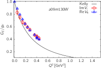
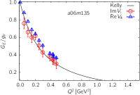
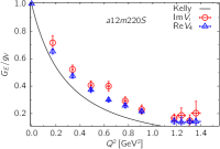
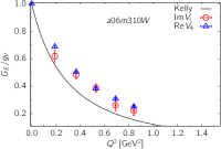
A consequence of this difference in the ESC behavior is that the errors in are 3–10 times larger than in (see data in Tables 2 and 3). Also, since one cannot extract a value for using the operators due to kinematic constraint, the fits to versus , discussed in Sec. V.2, are less stable because they are not anchored at . As a result, the extraction of the electric charge radius from the data has much larger errors. Because of these two reasons, it has been common to analyze only . With our high-statistics data, we are able to compare the ESC, the efficacy of the fits, and the discretization errors between and .
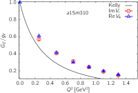
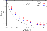
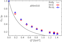
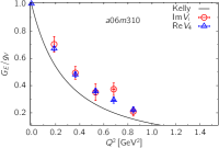
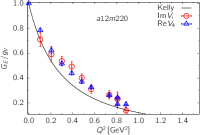
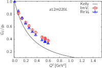
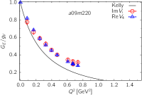
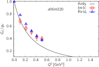
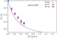
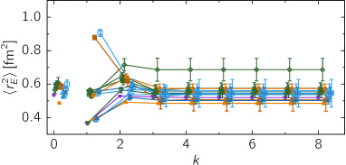
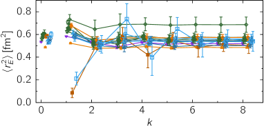
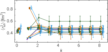
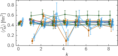
A comparison of results for and is presented in Fig. 1 for the thirteen calculations. As stated above, the errors in are much larger than those in , however, there are two additional noteworthy patterns. First, the data for for GeV2 on the , , and the two physical mass ensembles and , have the largest errors and mostly lie below those from . On the other hand, the data for GeV2 overlap in most cases. Our conclusion, based on these data, is that for GeV2 the two measurements can be considered to have the same mean but with different variance.
The pattern of data at GeV2 is puzzling and we do not have an explanation for the larger errors or the systematic differences. In particular, we cannot discern whether they are due to residual ESC, statistical fluctuations and/or different discretization errors. In summary, while our high-statistics data have allowed us to quantify the larger errors and fluctuations in , we do not have a resolution for the difference. Operationally, using a weighted average of the nonzero data from and , i.e., assuming that the differences are statistical fluctuations, gives results that are essentially identical to those from . We, therefore, analyze only the data from in the rest of this paper. To establish full control over all systematics, future calculations should demonstrate consistency between and .
IV.2 Extraction of
Examples of the size and shape of the ESC in the extraction of are shown in Figs. 28 and 29. For small momentum transfer, the convergence is monotonic from below as shown in Fig. 28 for . The ESC is observed to grow with decreasing and .
The pattern of convergence changes with : for small it is from below but by about , it has changed to from above in most cases as illustrated in Fig. 29. As a result, removing ESC increases the value of at small momentum transfers and decreases it at larger momenta. Consequently, if ESC is not removed, both the magnetic charge radius and the magnetic moment extracted are underestimated.
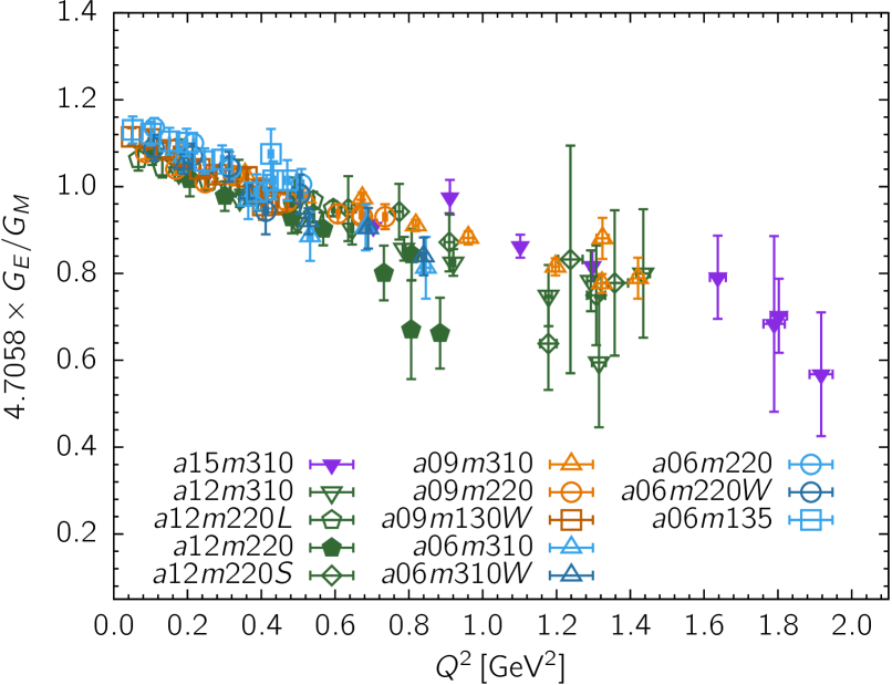
The results of the -fits to the data for the bare form factor are summarized in Table 4. A key shortcoming of the analysis of the lattice is the lack of data at . To overcome this, we note that the ratio , shown in Fig. 12, is, within errors, linear in for GeV2. We, therefore make a linear fit to the ratio of the form factor data, , with momenta up to to obtain an estimate for the renormalized . The corresponding unrenormalized values, which we call derived , are also given in Table 4. These values are indistinguishable from those obtained from taking a ratio of the two correlators and then making a linear fit versus to these data. Including these values of improved the stability of the -expansion fits. Note that, the extrapolation of , inclusion of the extrapolated value of , and the fit to are done within a single jackknife loop, therefore, the statistical errors are accounted for correctly.
To estimate the importance of using the derived point , which anchors the fits to data, especially on ensembles with largish values of the minimum , we performed the following test. We fit the nonzero data for to extract the value and the slope at for each ensemble. Comparing the value for from this fit with the data given in Table 2, we find the magnitude of the difference for the dipole and fit is between 0.01–0.04 for the 13 calculations. The difference in the slope, , compared to the data in Table 5 is up to 9% for the dipole fit and up to 20% for the fit. Based on this test, it is not unreasonable that an uncertainty of similar size can be present in the extraction of and . Thus, to get high precision results without resorting to a derived value for or without using priors, requires having data at smaller values of .
IV.3 Dependence of and on the lattice parameters
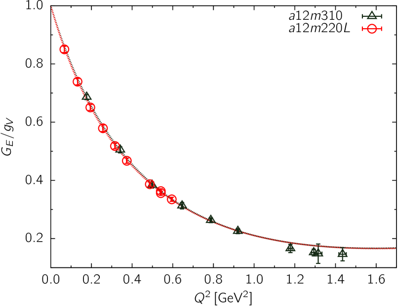
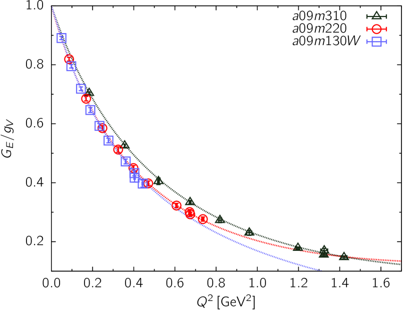
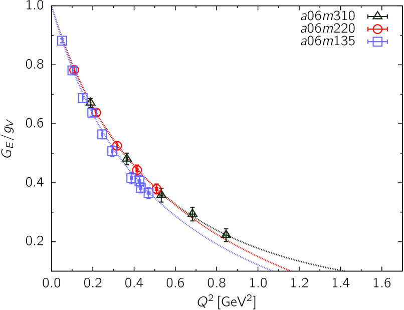
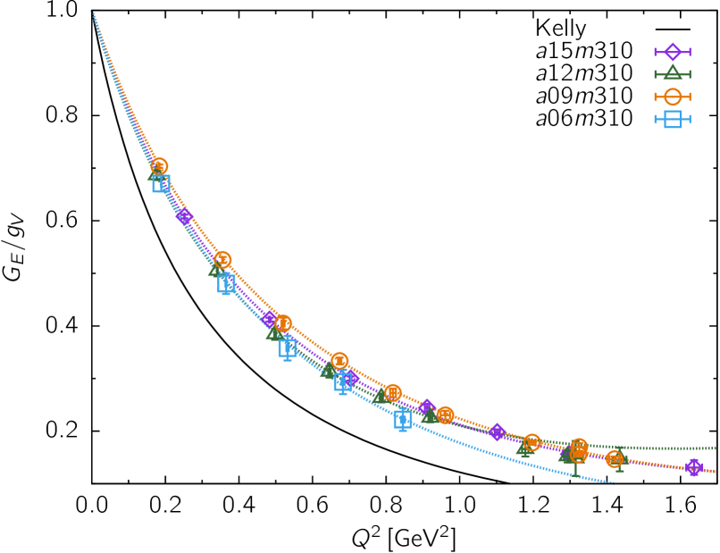
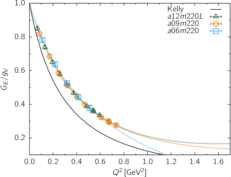
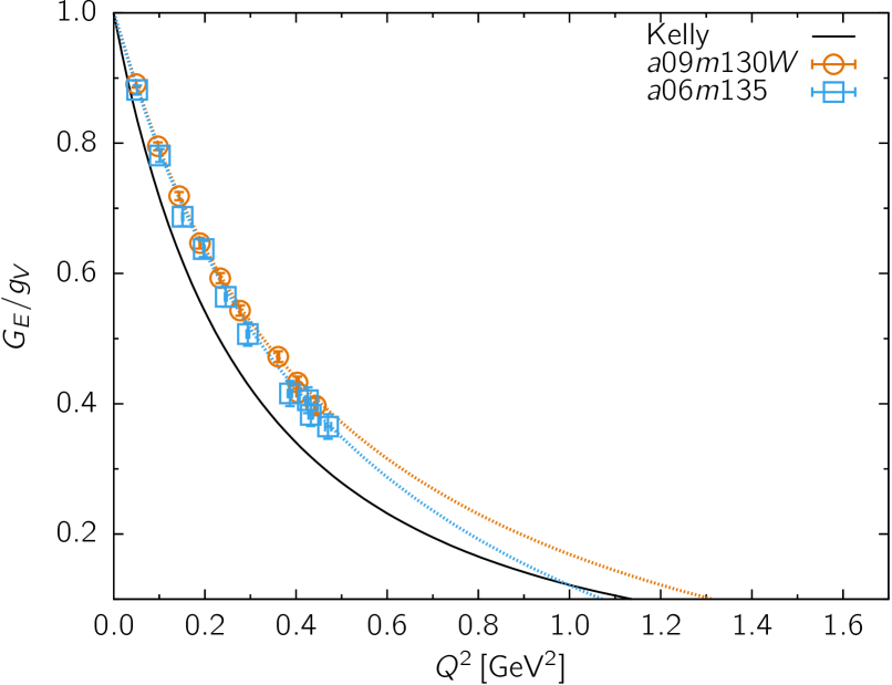
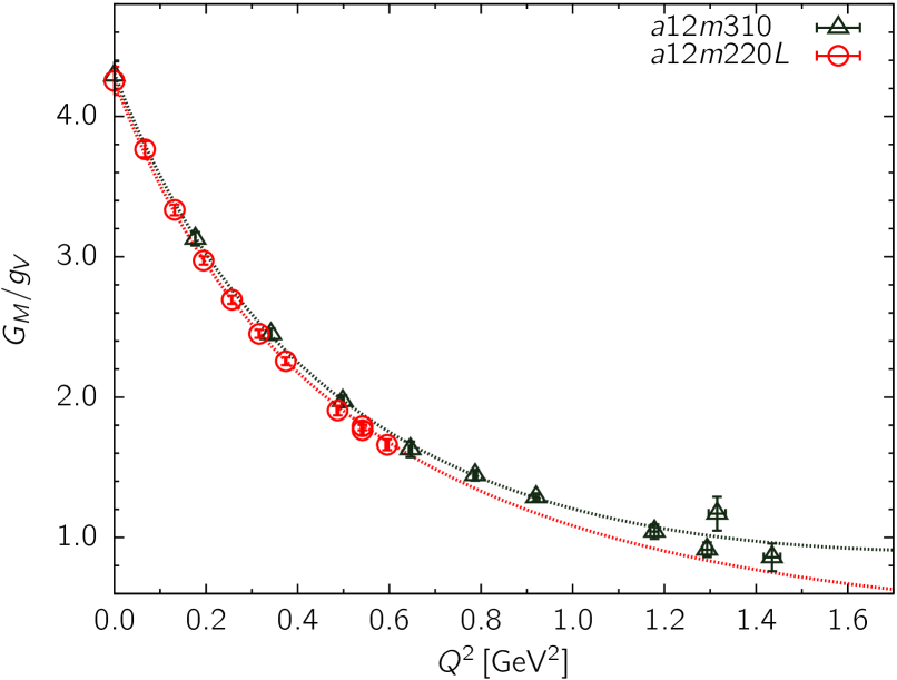
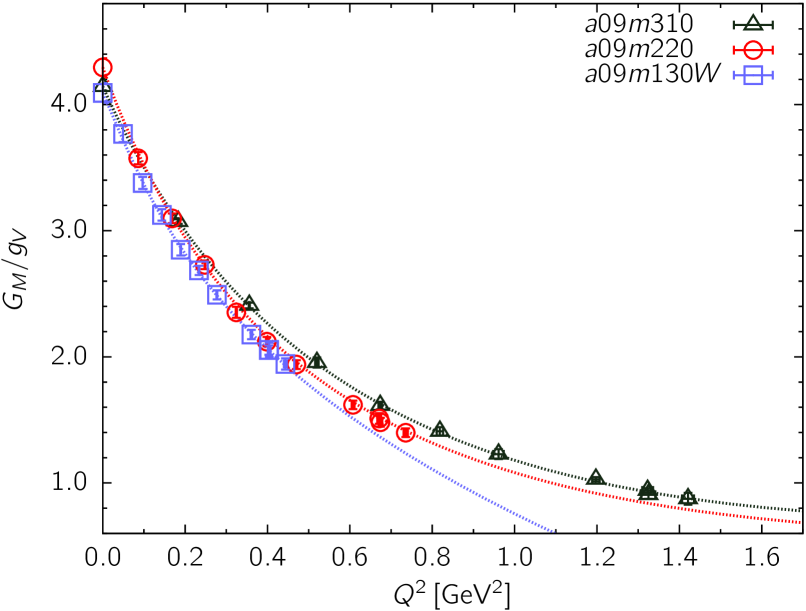
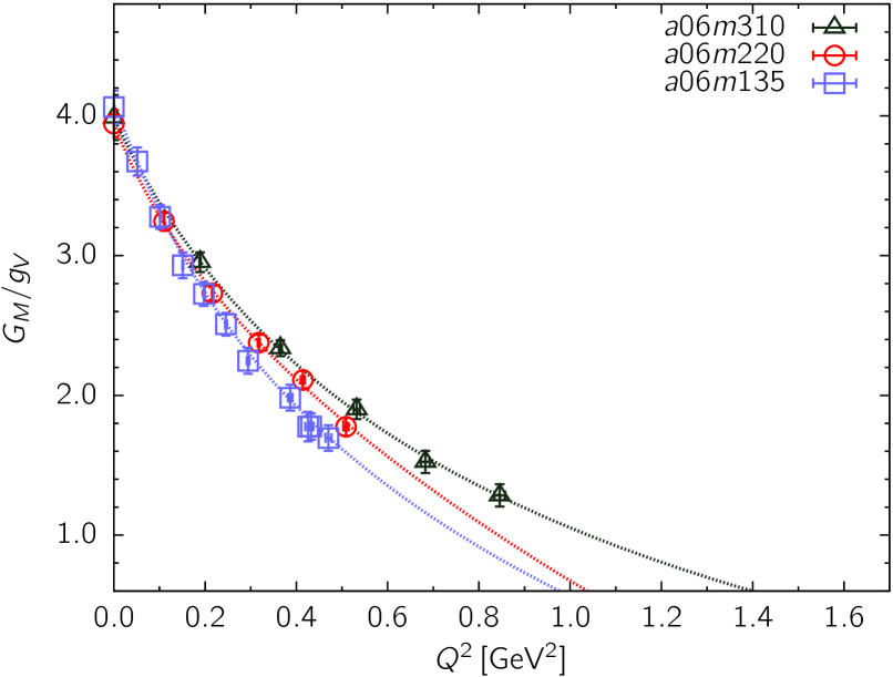
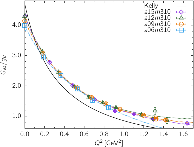
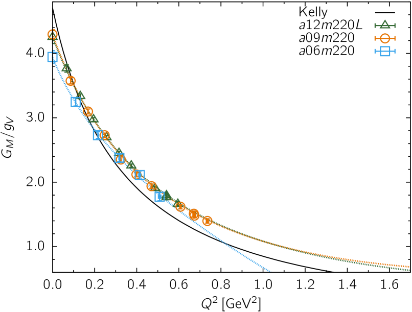
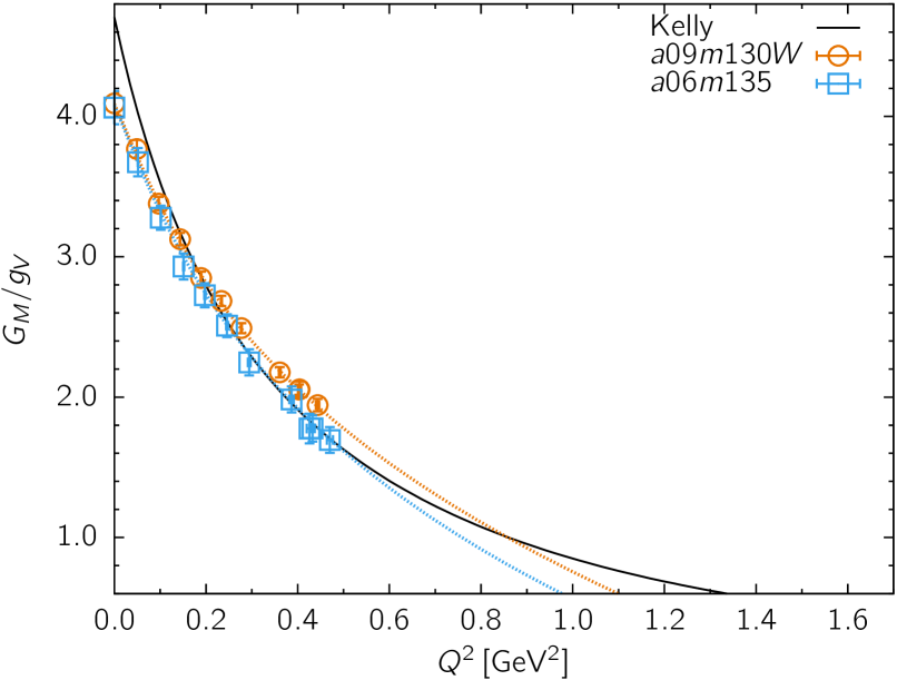
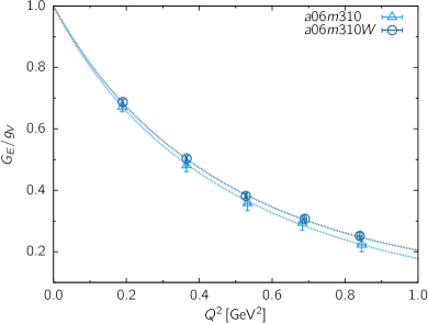
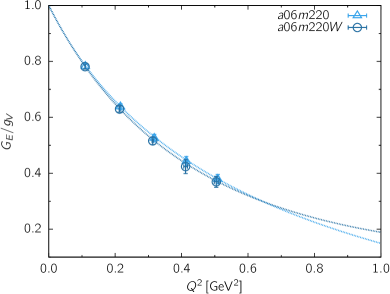
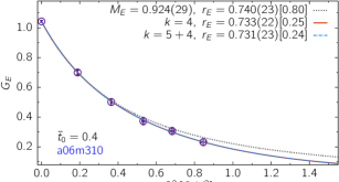
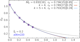
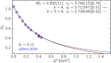
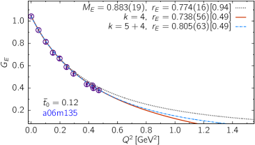
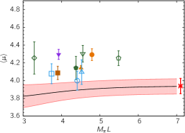
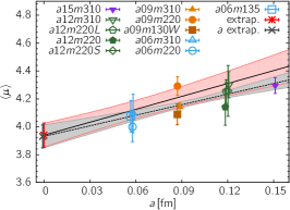
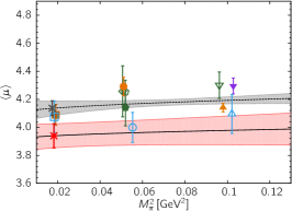
In Figs. 2–6, we explore the dependence of the renormalized form factors and , which we henceforth label and for brevity, as a function of the pion mass, lattice spacing, lattice volume and the smearing size. The significant features are:
- •
- •
Estimates for from -expansion fits without including our derived value for are, in many cases unstable even for the or fits, i.e., estimates for become negative. We conclude that the fits in these cases are over-parameterized. Including the derived value of and imposing the constraint on discussed in Sec. II greatly improved the -expansion fits. On the other hand, the dipole fits give consistent estimates with or without using a value for . Our final results for both types of fits are obtained including the points.
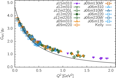
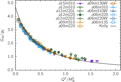
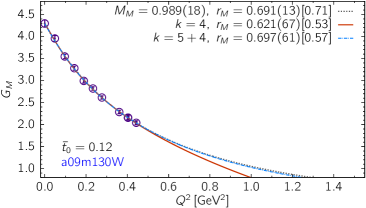
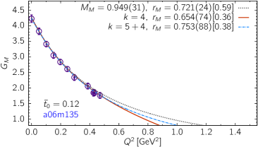
Lastly, the comparison of the lattice data with the Kelly fit to the experimental data is shown in Figs. 3 and 5. Both and move towards the Kelly curve as and are reduced. However, from the two physical mass ensembles still shows significant deviations from the Kelly fit. The data for show a different curvature from the Kelly curve and points with GeV from the physical mass ensembles move below the Kelly curve. This change in behavior in results in an underestimate of both and the magnetic moment as discussed in Sec. VI.
IV.3.1 Dependence on lattice size
Simulations on large lattices are not only important for reducing finite volume effects but also provide the simplest solution to obtaining data at smaller for fixed and . To demonstrate the improvement possible, we compare data from the , and ensembles in Fig. 30 in Appendix C. As the data move to smaller with increasing , the statistical quality of the signal also improves for a fixed number of measurements.
In Fig. 31, we show and versus for these three ensembles. The data on the two larger volumes, () and (), overlap for both and , indicating that finite volume effects are small for . On the smaller volume (), falls off faster with .
In Fig. 32, we compare the results of three fits to and given in Tables 2 and 4 versus for these three ensembles. For the -expansion fits, the results for and from the two larger volumes are consistent within , while those on differ. We find no significant difference in the dipole fits. These comparisons indicate that finite volume corrections are smaller than the statistical errors on the two larger volumes corresponding to . For this reason, we carry out CCFV fits including (11-point fit) and discarding the point (-point fit). Operationally, the fits are insensitive to the point due to the larger errors in it. Nevertheless, our final results, presented in Sec. VI, are from the 11-point fit.
The bottom line is that increasing for fixed and improves the analysis in a number of ways because the values of for a given decrease. First, the statistical errors for a fixed number of measurements decrease. The reduction in errors roughly compensates for the increase in cost of each measurement due to a larger volume. Second, with the decrease in , the ESC in becomes smaller, while that in becomes easier to control using n-state fits. Lastly, the extraction of , and improves since the fit parameters are determined from data with values of closer to zero.
IV.3.2 Dependence on smearing size
In Figs. 33 and 34 in Appendix C, we compare the ESC in and for two different smearing sizes using data from the and ensembles. The data show that the ESC is smaller with the larger smearing size.
The results of the dipole, and fits to and versus for these two ensembles are shown in Fig. 35. Results for and are consistent within for the two smearings. The data in Fig. 6, however, show that estimates of can differ by about 5% between the two calculations with different smearing size. This level of difference can be explained by a combination of statistical and possible systematic uncertainties.
IV.3.3 Dependence on lattice scale setting
The two places the lattice scale enters our calculation is in converting to physical units and in the CCFV fits. In Table 12, we give the values of for the HISQ ensembles obtained by the MILC collaboration using the Sommer scale Bazavov et al. (2013); Sommer (2014). In Table 14 in Appendix B, we give the value of obtained on each ensemble using these values of and fit them using the leading order CCFV fit defined in Eq. (29). The result in the continuum limit is MeV. The deviation of about 4% from the experimental value indicates a systematic uncertainty of 2–6% in the scale obtained from versus , the latter analyzed using the leading order CCFV fit. The question then is, how does this difference impact the analysis of the form factors and the extraction of , and ?
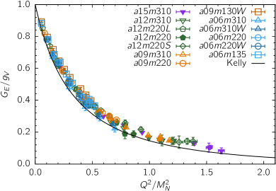
The lattice data plotted in Figs. 2–5 show that the dependence of the form factors on and is small. To explore the dependence further, we remove the use of taken from the analysis of the Sommer scale on the HISQ ensembles by plotting the data versus in Fig. 7 (bottom) where the lattice values of are used to construct the dimensionless ratio for the lattice data and MeV for the Kelly curve. The relative movement between the data and the Kelly curve, when plotted versus as compared to , brings the data closer together onto a single curve as can be seen by comparing the top and bottom set of panels. For the physical mass ensembles, the size of the relative movement of data depends only on the discretization errors, i.e., the value of at that value of , assuming finite volume corrections are negligible. Presuming a cancellation of some of the systematics when the data are plotted versus , this comparison indicates that the observed larger deviation from the Kelly curve, when the data are plotted versus , can be explained partly as a systematic effect due to discretization errors, i.e., variations in the lattice scale set using different observables. This systematic is avoided if data at a given are first extrapolated to MeV and and then compared with the Kelly curve. An attempt at doing this is described in Sec. VI.2.
It is important to note that , and extracted for each ensemble are unchanged whether one calculates them using or as the independent variable in Eq. (10). The result would be different if the product is calculated on each ensemble, and extrapolated to the continuum limit first, and the result divided by the experimental value for . We discuss this analysis in Sec. VI.1.
Having made clear that part of the noticeable spread in the behavior of the form factors shown in Fig. 7 can be accounted for, in a large part, as due to discretization errors, the question is–what is the more robust way of analyzing the data? Should we use the scale set using or work with dimensionless variables in units of ? While our analysis has exposed this systematic, our conclusion is that a larger data set, or the use of a lattice action with much smaller discretization errors or a better determined extrapolation ansatz are needed to significantly reduce such systematics. Having highlighted the size of this systematic uncertainty, most of the analysis presented below is carried out versus . We provide comparison with results plotted versus at appropriate places, and analyze data for and in Sec. VI.1.


V Characterizing the behavior of the form factors
In order to extract the charge radii defined in Eq. (10) and the magnetic moment in Eq. (8), we need to parameterize the form factors versus . The two fits we explore are the dipole and the -expansion truncated at some power as discussed in Sec. II. Since the dipole ansatz is the solution to an exponentially falling charge distribution (thus a model) and the -expansion involves a truncation plus a constraint on the size of the coefficients , it behooves us to first test these ansätze on the high-precision experimental data as discussed next.
V.1 Experimental data for the form factors and their behavior
Electromagnetic form factors of nucleons are extracted from differential cross-sections measured in the scattering of electrons off nuclei. The process of going from measurements of the differential cross-sections to nucleon form factors is nontrivial and involves modeling Perdrisat et al. (2007); Lee et al. (2015); Yan et al. (2018). As already stated, we have two reasons to analyze the experimental data: to compare them against the lattice data over the range GeV2, and to test the efficacy of the dipole and -expansion fit ansätze. For these purposes, we have collected together compiled experimental data for the proton and the neutron in Appendix D (see Figs. 36 and 37). From these, we have determined the Kelly parameterization for the isovector combinations, and . Henceforth, for brevity, we will continue to use and to represent the combinations when comparing the lattice and the experimental data.
Next, we test the fit ansätze on the experimental data. The results for and for the proton are shown in Fig. 36. Based on the , the dipole fit works surprisingly well for , and the deviation from the data is less than a percent over the range GeV2. This difference is far less than the precision of our lattice data. For , the deviation is larger (up to 6%) and the of the fit is poor. In the the -expansion fits with constraints, results for , and stabilize for as shown in Fig. 38.
Based on this analysis, and as noted in Appendix D, one should not expect a match between our lattice and the experimental data to better than about 5% or be able to resolve differences between the dipole and the -expansion fits at or below this level. These comparisons provide a framework for our lattice analyses using the -expansion: extract and from to avoid over-parameterization for some of the ensembles.
In the final estimates, we have assigned an additional systematic uncertainty to account for the fact that the CCFV fits have been made using just the leading order corrections. This is discussed further in Sec. VI.
V.2 Analysis of the lattice QCD data for the form factors
A comparison of the form factors and from all thirteen simulations with the Kelly parameterization of the experimental data is shown in Fig. 7. The data for lie above the Kelly curve with those from the two physical mass ensembles being the closest as shown in Fig. 3, whereas the data for lies about the Kelly curve for GeV2 and then falls below it for smaller as highlighted in Fig. 5. In both cases, these deviations from the Kelly curve impact the slope at , i.e., both and come out smaller than the phenomenological estimates. More importantly, the very precisely measured magnetic moment, , is underestimated by about 16%. As remarked above in Sec. IV.1 and Sec. IV.2, removing the ESC using the -fits increases the value of all three, nevertheless, the final results presented in Sec. VI are smaller than the experimental values. Furthermore, deviations of the lattice form factors from the Kelly curve are apparent over a range of .
As discussed in Sec. IV.3.3, part of the difference between the Kelly curve and the data is due to the mismatch in the scale set by and . This is highlighted in Fig. 7 where data are plotted versus (top panels), evaluated using the lattice scale set by , and versus the dimensionless variable (bottom panels). Note that this change of variable does not impact the results for , and on each individual ensemble and thus their extrapolated values.
The data for and versus are shown in Fig. 8. Our overall strategy for extracting , and is the following: We first determine by eye the largest value of up to which the data are smooth in . Next, since we are interested in the value and slope of the fits at , we restricted the data to GeV2, except for the ( GeV2) and ( GeV2) ensembles. The allowed range –, where is the largest value allowed by the cuts defined above, is marked by the two vertical red lines in Fig. 8. With these cuts, the points at all are retained for most of the ensembles. Only the high data for , , and ensembles are removed. These show a break in the smooth behavior in as is clear from Fig. 8. Going back to the ESC analysis, the reliability of these points is questionable since the data have large errors and the ESC fits were poor.
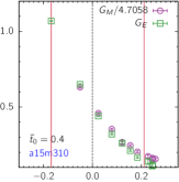
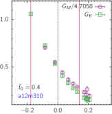
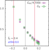
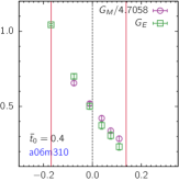
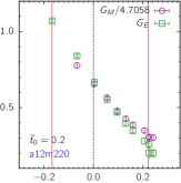
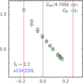
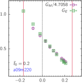
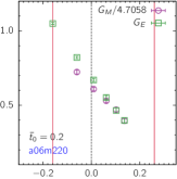
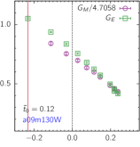
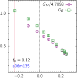
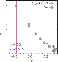
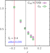
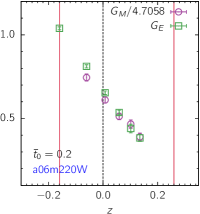
The results from the -expansion fits are stable for as shown in Fig. 9. Results from fits including the sum rules are similar, except that stability is reached only for . Estimates from fits with and without sum rules are consistent, however the errors are larger with the sum rules. The values and of the dipole fits have been stable under increase in statistics for all thirteen calculations. On the other hand, the results from the -expansion fits required high statistics to exhibit convergence with the order of the truncation.
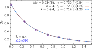
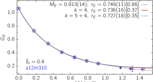
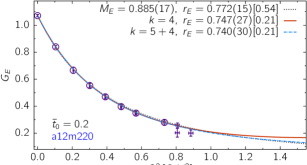
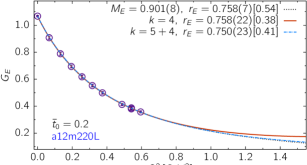
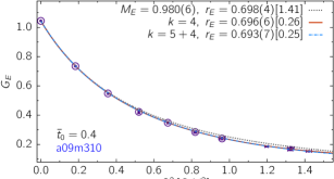
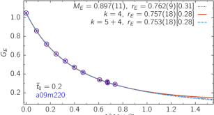
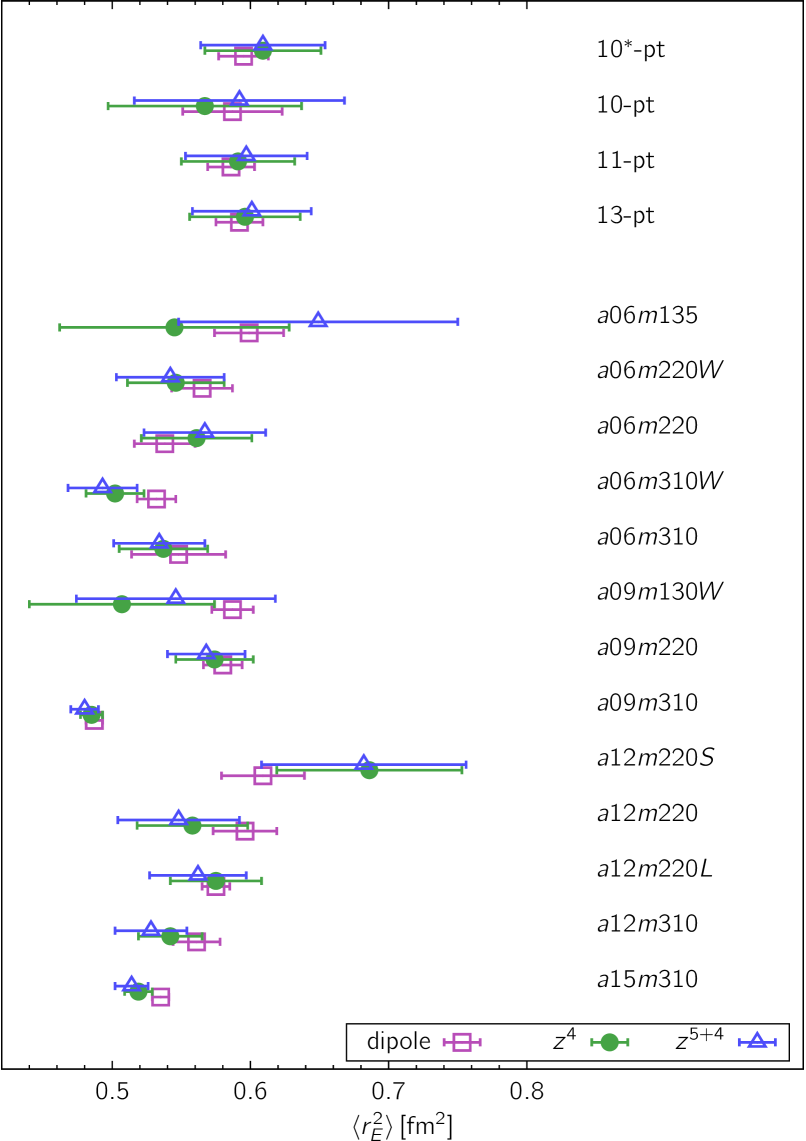
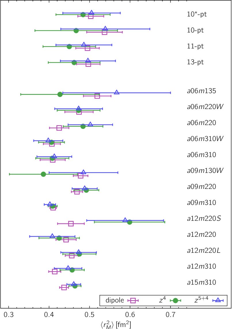
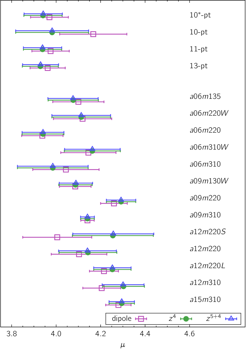
The results from seven fit ansatz are collected together in Tables 5, 6 and 7. Overall, the seven estimates are consistent within errors. Since , and should be extracted from the small behavior, our final results are from the fits. Estimates with sum rules are used only as consistency checks. The dipole, and fits and results are shown in Figs. 10 and 11 for ten ensembles.
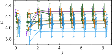
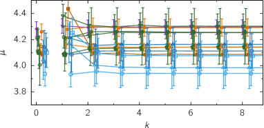
The data for the ratio are shown in Fig. 12. Experimental data indicate that this ratio for the proton is estimated to cross zero around GeV2 Punjabi and Perdrisat (2014). Our data for the isovector combination do show a negative slope over the region GeV2, nevertheless, data at larger are needed to determine if and where the ratio crosses zero. As discussed in Sec. IV.2, we have used this “linear” behavior at small to estimate from the ratio, including which helped stabilize the fits to . In the next section, we discuss the continuum-chiral-finite-volume (CCFV) fits used to get the physical estimates.
| Ensemble | Dipole | ||||||
|---|---|---|---|---|---|---|---|
| 0.535(6) | 0.523(10) | 0.519(10) | 0.519(10) | 0.492(17) | 0.531(8) | 0.514(12) | |
| 0.561(17) | 0.542(23) | 0.542(23) | 0.542(23) | 0.513(31) | 0.573(22) | 0.528(26) | |
| 0.575(10) | 0.562(32) | 0.575(33) | 0.575(33) | 0.574(45) | 0.588(32) | 0.562(35) | |
| 0.596(23) | 0.557(40) | 0.558(40) | 0.558(40) | 0.546(59) | 0.572(35) | 0.548(44) | |
| 0.609(30) | 0.686(69) | 0.686(67) | 0.686(67) | 0.688(93) | 0.690(57) | 0.682(74) | |
| 0.487(6) | 0.485(8) | 0.485(8) | 0.485(8) | 0.480(12) | 0.494(10) | 0.480(10) | |
| 0.580(14) | 0.575(26) | 0.574(28) | 0.573(28) | 0.566(31) | 0.576(29) | 0.568(28) | |
| 0.587(15) | 0.503(51) | 0.507(67) | 0.506(67) | 0.577(85) | 0.421(115) | 0.546(72) | |
| 0.548(34) | 0.537(32) | 0.537(32) | 0.537(32) | 0.533(41) | 0.542(36) | 0.534(33) | |
| 0.532(14) | 0.502(21) | 0.502(21) | 0.502(21) | 0.483(36) | 0.522(20) | 0.493(25) | |
| 0.538(22) | 0.560(40) | 0.561(40) | 0.561(40) | 0.604(57) | 0.543(35) | 0.567(44) | |
| 0.565(22) | 0.546(35) | 0.546(35) | 0.546(35) | 0.548(54) | 0.551(32) | 0.542(39) | |
| 0.599(25) | 0.529(64) | 0.545(83) | 0.545(82) | 0.735(135) | 0.398(159) | 0.649(101) | |
| 13-pt | 0.592(17) | 0.570(39) | 0.596(40) | 0.595(40) | 0.658(55) | 0.604(39) | 0.601(43) |
| 13-pt | 0.581(13) | 0.565(30) | 0.597(34) | 0.597(34) | 0.674(47) | 0.609(36) | 0.618(37) |
| 11-pt | 0.586(17) | 0.564(39) | 0.591(41) | 0.590(41) | 0.653(56) | 0.604(41) | 0.597(44) |
| 11-pt | 0.572(14) | 0.554(32) | 0.588(36) | 0.587(36) | 0.665(49) | 0.606(39) | 0.609(39) |
| 10-pt | 0.587(36) | 0.552(69) | 0.567(70) | 0.567(70) | 0.632(93) | 0.530(68) | 0.592(76) |
| 10-pt | 0.558(24) | 0.540(48) | 0.570(53) | 0.570(53) | 0.662(74) | 0.554(58) | 0.618(59) |
| 10∗-pt | 0.595(18) | 0.587(40) | 0.609(42) | 0.608(42) | 0.668(57) | 0.607(41) | 0.609(45) |
| 10∗-pt | 0.571(14) | 0.546(32) | 0.577(36) | 0.577(36) | 0.657(50) | 0.587(40) | 0.600(40) |
| Ensemble | Dipole | ||||||
|---|---|---|---|---|---|---|---|
| 0.437(11) | 0.466(15) | 0.464(15) | 0.464(15) | 0.451(23) | 0.472(13) | 0.461(17) | |
| 0.414(15) | 0.457(30) | 0.457(30) | 0.457(30) | 0.438(41) | 0.484(28) | 0.447(34) | |
| 0.456(16) | 0.475(41) | 0.475(41) | 0.475(41) | 0.485(58) | 0.472(39) | 0.473(44) | |
| 0.442(25) | 0.419(51) | 0.425(50) | 0.424(50) | 0.406(74) | 0.451(46) | 0.408(56) | |
| 0.454(33) | 0.597(89) | 0.599(87) | 0.599(87) | 0.566(118) | 0.617(77) | 0.588(95) | |
| 0.410(8) | 0.409(11) | 0.409(11) | 0.409(11) | 0.400(17) | 0.423(12) | 0.402(14) | |
| 0.469(14) | 0.489(30) | 0.492(31) | 0.492(31) | 0.498(38) | 0.499(32) | 0.488(31) | |
| 0.478(18) | 0.437(56) | 0.386(84) | 0.384(83) | 0.478(132) | 0.092(173) | 0.485(85) | |
| 0.409(31) | 0.408(41) | 0.408(41) | 0.408(41) | 0.436(55) | 0.396(46) | 0.413(43) | |
| 0.407(21) | 0.406(32) | 0.406(32) | 0.405(32) | 0.388(52) | 0.416(33) | 0.398(36) | |
| 0.425(24) | 0.485(49) | 0.484(49) | 0.484(49) | 0.546(78) | 0.438(44) | 0.502(55) | |
| 0.474(35) | 0.473(53) | 0.473(53) | 0.473(53) | 0.477(88) | 0.465(48) | 0.473(59) | |
| 0.519(34) | 0.456(76) | 0.427(97) | 0.427(97) | 0.634(214) | 0.115(195) | 0.567(133) | |
| 13-pt | 0.497(29) | 0.454(61) | 0.462(64) | 0.461(64) | 0.560(90) | 0.443(65) | 0.496(68) |
| 13-pt | 0.482(19) | 0.449(41) | 0.458(49) | 0.457(49) | 0.575(77) | 0.441(59) | 0.520(54) |
| 11-pt | 0.495(29) | 0.445(62) | 0.450(65) | 0.449(65) | 0.548(92) | 0.434(67) | 0.486(69) |
| 11-pt | 0.480(20) | 0.436(43) | 0.443(51) | 0.441(51) | 0.558(80) | 0.432(63) | 0.505(56) |
| 10-pt | 0.537(44) | 0.471(100) | 0.467(102) | 0.466(102) | 0.617(141) | 0.363(102) | 0.539(110) |
| 10-pt | 0.497(28) | 0.444(62) | 0.447(71) | 0.446(71) | 0.610(112) | 0.378(87) | 0.549(80) |
| 10∗-pt | 0.503(32) | 0.481(65) | 0.484(67) | 0.484(67) | 0.563(94) | 0.449(67) | 0.505(71) |
| 10∗-pt | 0.480(20) | 0.431(43) | 0.433(52) | 0.432(51) | 0.550(80) | 0.407(64) | 0.498(57) |
| Ensemble | Dipole | ||||||
|---|---|---|---|---|---|---|---|
| 4.280(57) | 4.295(57) | 4.295(57) | 4.295(57) | 4.296(57) | 4.296(57) | 4.295(57) | |
| 4.205(85) | 4.303(94) | 4.303(94) | 4.303(94) | 4.297(94) | 4.310(94) | 4.301(94) | |
| 4.215(65) | 4.253(84) | 4.253(84) | 4.253(84) | 4.257(85) | 4.252(83) | 4.253(84) | |
| 4.103(125) | 4.143(130) | 4.143(130) | 4.143(130) | 4.134(130) | 4.135(130) | 4.141(130) | |
| 4.005(155) | 4.256(182) | 4.255(182) | 4.255(182) | 4.262(182) | 4.262(182) | 4.257(182) | |
| 4.141(30) | 4.141(31) | 4.141(31) | 4.141(31) | 4.141(31) | 4.140(31) | 4.141(31) | |
| 4.260(60) | 4.292(66) | 4.292(66) | 4.292(66) | 4.291(66) | 4.292(67) | 4.292(66) | |
| 4.086(71) | 4.088(75) | 4.087(75) | 4.087(75) | 4.095(74) | 4.084(75) | 4.089(75) | |
| 4.044(149) | 3.985(159) | 3.985(159) | 3.985(159) | 3.989(157) | 3.986(160) | 3.985(159) | |
| 4.145(124) | 4.163(126) | 4.163(126) | 4.163(126) | 4.163(125) | 4.161(126) | 4.163(125) | |
| 3.938(93) | 3.941(94) | 3.941(94) | 3.941(94) | 3.940(94) | 3.941(94) | 3.941(94) | |
| 4.119(131) | 4.113(132) | 4.113(132) | 4.113(132) | 4.113(132) | 4.112(132) | 4.113(132) | |
| 4.100(115) | 4.078(113) | 4.077(113) | 4.077(113) | 4.078(112) | 4.079(113) | 4.076(113) | |
| 13-pt | 3.962(79) | 3.930(81) | 3.929(81) | 3.929(81) | 3.932(81) | 3.927(81) | 3.930(81) |
| 13-pt | 3.950(79) | 3.918(80) | 3.917(80) | 3.917(80) | 3.920(80) | 3.915(80) | 3.917(80) |
| 11-pt | 3.975(84) | 3.940(86) | 3.939(86) | 3.939(86) | 3.942(86) | 3.937(86) | 3.939(86) |
| 11-pt | 3.968(84) | 3.933(86) | 3.932(86) | 3.932(86) | 3.935(85) | 3.930(86) | 3.933(86) |
| 10-pt | 4.167(151) | 3.982(164) | 3.982(164) | 3.982(164) | 3.987(164) | 3.976(164) | 3.982(164) |
| 10-pt | 3.999(122) | 3.879(129) | 3.877(129) | 3.877(129) | 3.884(129) | 3.874(129) | 3.879(129) |
| 10∗-pt | 3.970(85) | 3.942(86) | 3.941(86) | 3.941(86) | 3.945(86) | 3.940(86) | 3.942(86) |
| 10∗-pt | 3.964(84) | 3.933(86) | 3.932(86) | 3.932(86) | 3.936(85) | 3.930(86) | 3.933(86) |
VI Results for , and
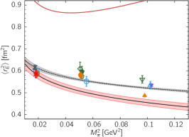
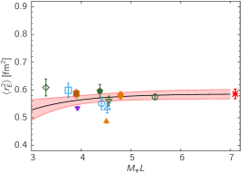
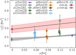

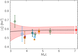
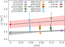
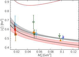
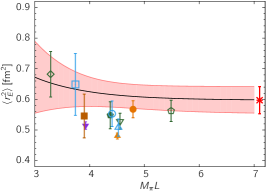
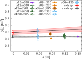
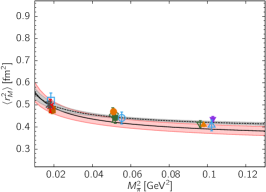
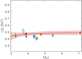
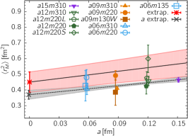
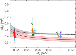


To obtain results for , and in the limits , MeV and , we make a simultaneous (CCFV) fit in these three variable to the data given in Tables 5, 6 and 7. Given the spread in the lattice parameters of the 11 ensembles analyzed, we include the leading order correction term in each of the three variables, i.e., fits with four free parameters, . The fit ansatz for the electric mean-square charge radius used is
| (25) |
where the mass scale is chosen to be and the form of the chiral and FV corrections are taken from Refs. Bernard et al. (1998); Kubis and Meissner (2001); Gockeler et al. (2005). For the magnetic mean-square charge radius, we use
| (26) |
where the leading dependence on is taken from Ref. Bernard et al. (1998); Kubis and Meissner (2001). Lastly, the ansatz used for the magnetic moment is
| (27) |
where the forms of the chiral and finite volume correction terms are taken from Ref. Kubis and Meissner (2001); Beane (2004). We express all masses in units of GeV and the lattice spacing in fm.
In all three CCFV fit ansatz, Eqs. (25)–(27), heavy baryon chiral perturbation theory (PT) has been used only to determine the form of the leading order chiral correction. For example, for , PT predicts the slope, , of the linear dependence on as with MeV Beane and Savage (2003), however, we leave a free parameter. For and , we do not have data at enough values of to test the contribution of the different terms in the PT prediction Kubis and Meissner (2001) as discussed later in this section. To avoid over parameterization of the fit we, therefore, include only the nonanalytical term in Eqs. (25) and (26). Our focus is on obtaining estimates at MeV, and this is achieved by relying on the data from the two physical mass ensembles to anchor the chiral part of the fit.
In Tables 5, 6 and 7, we also give the results of the CCFV fits for the following four combinations of the thirteen data points:
-
•
13-point fit. All the thirteen calculations as considered to be independent, even though the a06m310 and a06m220 ensembles have been analyzed twice with different smearing sizes.
-
•
11-point fit. We use the average of the two values for , and on the and ensembles as these have been analyzed twice. In this averaging, we assume maximum correlation between data
-
•
10-point fit. We remove the coarsest ensemble, , from the eleven data points defined above.
-
•
-point fit. We remove the smallest volume ensemble, , from the eleven data points defined above.
For each of these fits, we give results with (labeled extrap ) and without (labeled extrap ) the finite volume correction. The values of the coefficients are given in Table 8. In the limit and , only the terms proportional to and contribute. From these fits, we observe the following:
-
•
Of our estimate fm2, roughly half comes from and the other half from . Compared to the experimental value fm2 (see Eq. (30)), about fm2 is missing.
-
•
Of fm2, roughly 60% comes from and the rest from . Compared to the experimental value fm2 (see Eq. (30)), about fm2 is missing.
-
•
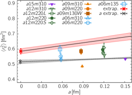
There is a significant dependence of on the lattice spacing . As a result, we get a low value, Bohr magneton, in the continuum limit.
-
•
The coefficient of the finite volume term is poorly determined, which is reflected in the larger error estimates with . In all cases, the two types of results overlap. To be conservative, we quote all final results including the finite volume term.
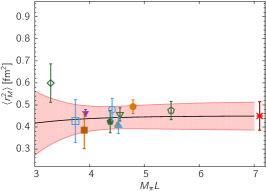
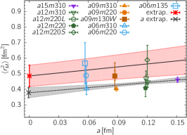
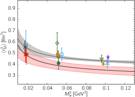
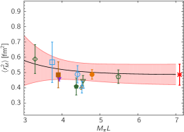
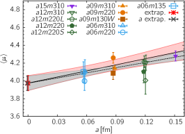
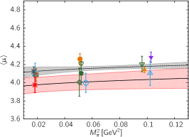
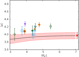
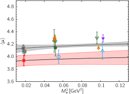
In Figs. 13, 14 and 15, we show the CCFV fits versus , and for three analyses: dipole, and . In addition, we show fits versus a single variable or (gray bands). When the pink and gray bands are close or overlap, it means that the dominant sensitivity of the CCFV fit is with respect to the single variable of the gray band.
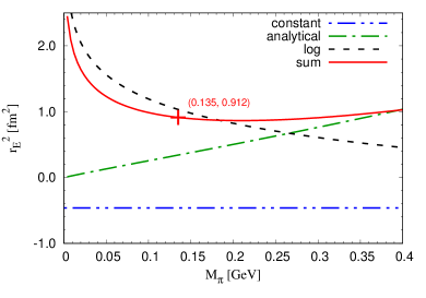
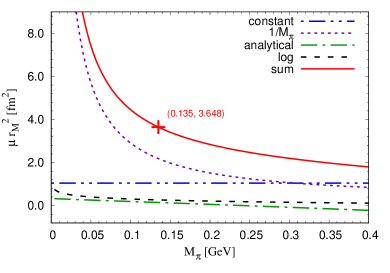
For , we also show the fit using the PT expression given in Ref. Kubis and Meissner (2001) as a solid red line in Fig. 13. The variation with in the dipole, and the data is small over the range MeV, and consistent with the prediction of PT. The singular behavior is expected to dominate for MeV. As shown in Fig. 16, over the range MeV, the decrease in the “log” part is partially compensated for by the increase in the “analytical” contribution as .
The shape of the CCFV fit bands are similar for the dipole, and the , except that the -expansion data and the fits have larger errors. A visual overview of all 13 individual results for and of the four CCFV fits is presented in Fig. 17. The variation with and in the thirteen individual calculations is small and somewhat smaller in the dipole than in the various -expansion estimates.
| (fm2) | (fm) | (fm2) | (fm2) | |
|---|---|---|---|---|
| dipole | 0.32(3) | 0.62(12) | -0.08(1) | 0.33(26) |
| 0.31(5) | 0.50(23) | -0.08(2) | 0.11(69) | |
| (fm2) | (fm) | (fm2 GeV) | (fm2 GeV) | |
| dipole | 0.31(3) | 0.32(18) | 0.024(6) | -0.14(19) |
| 0.28(6) | 0.77(32) | 0.023(15) | -0.09(48) | |
| (fm-1) | (GeV-1) | (GeV-1) | ||
| dipole | 3.93(11) | 2.28(89) | 0.33(40) | -44(39) |
| 3.91(11) | 3.10(98) | 0.22(42) | -51(45) |
For , the variation with , and for each of the three cases, the dipole, and the , is small as shown in Figs. 14 and 18. Presumably, the expected chiral behavior (see Eq. (26)) sets in at MeV. Again, the CCFV fits for the three cases shown in Fig. 14 are similar.
The largest variation in is versus as shown in Fig. 15. Again, the fit bands are similar for the dipole, and the data. The positive slope versus lowers the continuum limit result with respect to the experimental value . The size of the difference between lattice data and experimental results suggests that discretization and other systematic errors in are underestimated. From the summary of the results presented in Fig. 19, it is clear that the largest uncertainty is in the smallest volume, , and the two physical mass, a09m130W and , points.
It is instructive to compare our data to the predictions of chiral perturbation theory shown in detail Fig. 16. The chiral expansion for the isovector and , given in Ref. Kubis and Meissner (2001), are shown as the sum of three terms: those independent of (labeled constant), proportional to (labeled log) and the remaining terms proportional to powers of (labeled analytical). In making these plots, the low energy constants (LEC) used are GeV-1, , , , and MeV.
For , the “constant” term is negative ( fm2). In the range 135-350 MeV, is approximately constant at fm2: in this interval, the growth in the term compensates for the decrease in the “analytical” terms. Below , the log term drives the rise in the sum. As shown in Fig. 13, lattice data are significantly smaller in magnitude but show a similar small variation between – MeV. Because of this small variation, and having data at only three values, even including an additional analytical term proportional to just in our CCFV fits would over-parameterize the fit. Furthermore, over this range, a simple term would equally well mimic the sum of the log and the analytical terms. For this reason, we have included only one of the possible dependent terms, the log, in our CCFV fits.
In the case of shown in Fig. 16 (right), the “log” and “analytical” terms are small and the “log” shows little variation. The dominant contribution comes from the and “constant” terms. Since the term provides the largest variation with , we have only included it in the CCFV fit defined in Eq. (26).
In short, even though the PT based expressions used for both and , given in Eqs. (25) and (26), use only the leading chiral correction term from the expressions in Ref. Kubis and Meissner (2001), the variation in our data at three values of between 135–315 MeV is small, and including more terms would result in over-parameterization. In this situation, having lattice data at MeV, is crucial for controlling the uncertainty in the chiral fit to the lattice data. Note that the errors we quote in the CCFV fit results are comparable to those in the two physical mass points.
As is evident from the data in Tables 5, 6 and 7, and shown in Fig. 9, the -expansion results without sum rules converge for . Since , and should ideally be extracted from the small behavior, our final results are obtained as follows: We take the result for the central value and the first error in it represents the analysis uncertainty, i.e., including the ESC, and CCFV fits. We also quote a second systematic uncertainty to account for having used just the leading order CCFV fits. This is taken to be the largest of the following:
-
•
The difference between the two values on the physical mass ensembles, and . The second error estimate for is given by this difference.
-
•
The difference between the value at and the continuum value given by the CCFV fit. This gives the second error estimate for and for , which show the largest variation versus .
-
•
For the -expansion, we also considered the difference between the () and values. These turn out to be smaller than the estimates from the previous two cases.
The final results, obtained by applying this prescription to the 11-point CCFV fit values summarized in Tables 5, 6 and 7, are given in Table 9. For completeness, we also give the results for the Dirac and Pauli radii derived from these and using Eq. (12) in Table 9.
| (fm2) | (fm) | (fm2) | (fm) | (Bohr Magneton) | |
| dipole fit | 0.586(17)(13) | 0.765(11)(8) | 0.495(29)(41) | 0.704(21)(29) | 3.975(84)(125) |
| fit | 0.591(41)(46) | 0.769(27)(30) | 0.450(65)(102) | 0.671(48)(76) | 3.939(86)(138) |
| Combined fit | 0.564(114) | 0.751(76) | 0.459(189) | 0.678(140) | 3.922(83) |
| (fm2) | (fm) | (fm2) | (fm) | ||
| dipole fit | 0.389(18)(15) | 0.623(15)(12) | 0.531(44)(63) | 0.729(30)(43) | |
| fit | 0.396(42)(49) | 0.629(33)(37) | 0.469(90)(141) | 0.685(66)(103) | |
| Combined fit | 0.370(115) | 0.609(94) | 0.490(258) | 0.700(184) |
The central values for , and are about 17%, 19% and 16% smaller than the phenomenological values given in Eq. (30) and the precise experimental value in Eq. (9). Estimates from the dipole and -expansion fits, given in Table 9, are consistent, however, the errors in and from the -expansion fits are much larger, and about half the difference from the experimental/phenomenological values. The errors in the dipole fits are small compared to the difference between the lattice and the phenomenological/experimental estimates. As discussed in a number of places above, differences between the lattice and phenomenological estimates can be accounted for if a linear combination of the statistical and the various systematic errors is taken.
The encouraging results from our analysis are: (i) the data for both and is seen to converge towards the Kelly parameterization as and are decreased; (ii) the stability of the -expansion fits improves with statistical precision, however constraints on the coefficients are still needed; (iii) while it is hard to test the nonanalytical chiral behavior predicted in Eqs. (25) and (26) with data at only three values of , having data at the two physical mass ensembles anchors the CCFV fit and provides control over the uncertainty in values obtained from the fits.
A weakness of the lattice analysis is that cannot be calculated directly due to kinematic constraints. We have motivated the use of a derived value of to stabilize fits to . Looking ahead, the most significant improvement needed for extracting all three quantities with higher precision is generating data at smaller values of . This, unfortunately, requires ensembles with larger spatial volumes and/or new approaches such as a lattice formulation of the Dirac action with twisted boundary conditions de Divitiis et al. (2004); [ALPHA 01] R. Frezzotti et al. (2001). Both options are beyond the scope of this work as they require new simulations.
Two variants of the analysis presented above are described briefly next.
VI.1 Analysis of and
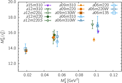
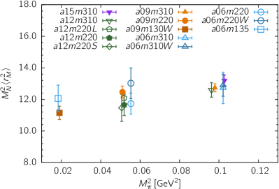
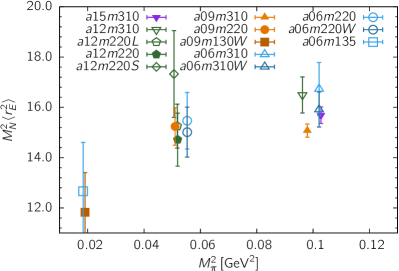
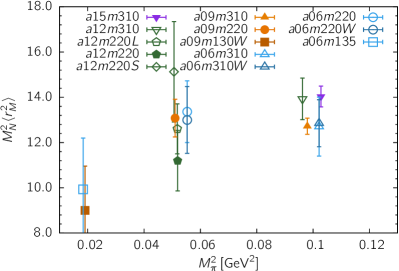
The dimensionless quantities and are plotted in Fig. 20 versus . For comparison, the phenomenological values for the isovector mean-square charge radii given in Eq. (30), imply and . A priori, if some of the systematics cancel in the product, then one would get smaller variation with and . The data for and in Fig. 20 show that there is significant variation with . Lacking a well motivated fit ansatz, a reasonable option is to take the average of the values from the two physical mass ensembles. These estimates are again low: , , , and . Multiplying the results given in Table 9 by fm-2 gives similar values. Given that the errors are also similar and because these estimates neglect possible dependence, we do not find this variant of the analysis as providing an obvious improvement.
VI.2 Combined CCFV Fit
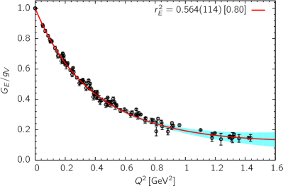
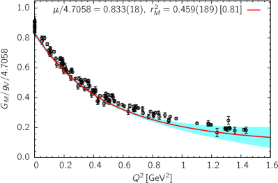
We also carried out a combined CCFV fit to the and data from the 13 calculations using a product of the -expansion for the behavior and the functional forms for the CCFV ansatz given in Eqs. (25) and (26):
| (28) |
Here represents the vector of variables in the CCFV fit, and each coefficient of the -expansion has a CCFV expansion of the form given in Eq. (25) or in Eq. (26). For example, for the four term CCFV ansatz given in Eqs. (25), , the combined fit has twenty parameters for the analysis. In performing these fits, we used Gaussian priors with mean 0 and width 5, in their appropriate units, for all the parameters. The resulting central values of the parameters were within this range.
The central values of the results with and without the finite volume term are consistent, however, the errors with the finite volume correction term included are about a factor of two larger. In Fig. 21, we show, for the case, the combined fits neglecting the finite volume correction term. The results of these combined fits are summarized in Table 9, and found to be consistent with those obtained by doing the and CCFV fits separately (labeled -fit).
VII Comparison with Previous Work
There have been a number of lattice QCD calculations of electric and magnetic isovector form factors of the nucleon. Recent ones include LHPC’14 Green et al. (2014), Mainz’15 Capitani et al. (2015), LHPC’15 Green et al. (2015), ETMC’17 Alexandrou et al. (2017b), LHPC’17 Hasan et al. (2018), PACS’18 Ishikawa et al. (2018), PACS’18A Shintani et al. (2019) and ETMC’18 Alexandrou et al. (2018). In this work, we restrict the comparison to calculations that have presented results at or near the physical pion mass. Their lattice parameters are given in Table 10 and the data for and are plotted in Fig. 22. We focus on comparing the data for and as these are the primary quantities calculated. Since the calculations have been done with different lattice actions, the data, even at the physical pion mass, are only expected to agree in the continuum limit. We find that, in fact, they agree remarkably well, much better than our analyses of various systematics would indicate.
| Ensemble ID | (fm) | (MeV) | Action | |||||
| (this work) | 0.0871(6) | 138(1) | 3.90 | 1290 | 165,120 | clover-on-2+1+1-HISQ | ||
| (this work) | 0.0570(1) | 136(2) | 3.7 | 675 | 43,200 | clover-on-2+1+1-HISQ | ||
| LHPC’17 Hasan et al. (2018) | 0.093 | 135 | 4.08 | 442 | 56,576 | 2+1-clover | ||
| ETMC’18 Alexandrou et al. (2018) | 0.0809(4) | 138(1) | 3.62 | 750 | 3K48K | 2+1+1-Twisted Mass | ||
| ETMC’17 Alexandrou et al. (2017b) | 0.0938(3) | 130(1) | 2.98 | 578725 | 9K64K | 2-Twisted Mass | ||
| ETMC’18 Alexandrou et al. (2018) | 0.0938(3) | 130(2) | 3.97 | 3331040 | 5K17K | 2-Twisted Mass | ||
| PACS’18 Ishikawa et al. (2018) | 0.0846(7) | 146 | 6.01 | 200 | 12,800 | 2+1-clover | ||
| PACS’18A Shintani et al. (2019) | 0.0846(7) | 135 | 7.41 | 20 | 2.5K10K | 2+1-clover |
| Ensemble ID | (MeV) | from | Fit | (fm) | (fm) | |
| 953(4) | 0.769(27)(30) | 0.671(48)(76) | 3.94(9)(14) | |||
| 951(10) | 0.765(11)(8) | 0.704(21)(29) | 3.98(8)(13) | |||
| LHPC’17 Hasan et al. (2018) | 912(8) | 0.887(49) | 4.75(15) | |||
| ETMC’18 Alexandrou et al. (2018) | 929(6) | dipole | 0.802(19)(12)(1) | 0.714(26)(88)(16)() | 3.96(14)(3)(7)() | |
| ETMC’17 Alexandrou et al. (2017b) | 941(2) | dipole | 0.808(30)(19) | 0.732(36)(45) | 4.02(21)(28) | |
| PACS’18 Ishikawa et al. (2018) | 958(10) | 0.915(99) | 1.437(409) | 4.81(79) | ||
| PACS’18A Shintani et al. (2019) | 942(11) | dipole | 0.875(15)(28) | 0.805(32)(274) | 4.417(138)(317) |
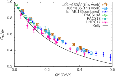
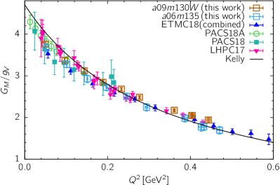
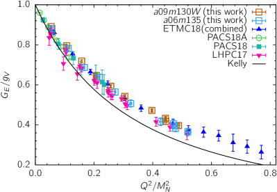
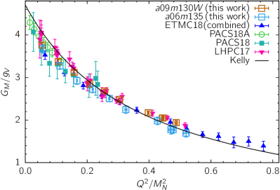
All the data included in the comparison are shown in the upper two panels in Fig. 22. From the plot versus , we draw the following overall conclusions:
-
•
The data approach the Kelly curve from above, while from below for GeV2.
-
•
No significant dependence on the number of flavors or the lattice spacing is manifest.
-
•
The PACS’18A data at GeV2, obtained using a large volume, show a qualitatively different behavior and lie closer to the Kelly curve. In this range of , the data are almost linear and highly correlated. They give a larger slope in both and and thus larger and .
-
•
We can also compare data at and 0.1 GeV2 from our and ensembles, from ETMC’18 Alexandrou et al. (2018), and the low error LHPC’17 Hasan et al. (2018) points with that from PACS’18A. Given the size of the statistical and systematic errors in individual data points, it is not clear if the observed small differences are significant at these two values.
Two points become clear on plotting the data versus , as shown in the bottom two panels of Fig. 22. First, the collapse of all data into a single curve over the whole range GeV2 becomes even more pronounced. Second, the deviation of this common curve from the Kelly curve is smaller. Thus, not only do all our data from the 13 calculations fall on a common curve when plotted versus , as shown in Fig. 7, but so do data from four other collaborations using different lattice actions and volumes. A priori, a common curve would suggest that all the systematics cancel, and the apparent differences between the various calculations when the data are plotted versus was largely a consequence of how the lattice scale is set.
Deviations from the Kelly curve are, however, significant in for GeV2. Data for data undershoot for GeV2 and are consistent with the Kelly curve above it. These differences are a 2–3 effect, and comparable to the size of the shift when the data are plotted versus or . While an understanding of how the different systematics contribute, and whether there is one that dominates requires future more detailed calculations, we remind the reader that during the course of our analyses, we have pointed out systematics, for example due to ESC and the deteriorating signal in both the 2- and 3-point correlation functions at large , could give rise to uncertainties of this size.
We have already shown that the pattern of ESC in our data is sensitive to the value of . In particular, as discussed in Sec. IV, the ESC in correlators from which is extracted increases with momentum and the convergence is from above. On the other hand, it is large at small in correlators from which we get and the convergence is from below. Thus, possible residual ESC could account for the observed deviation from the Kelly curve.
For , there is a clear benefit to performing calculations at small . As illustrated in Figs. 24 and 25 for the physical mass ensembles, the ESC in is still small for corresponding to GeV2. (Note that for , the ESC is essentially zero as the vector charge is conserved and the local current has no correction in forward matrix elements.) There is, however, an increase in the ESC with decreasing as shown in the bottom panels in Fig. 26. On the other hand, the ESC in is large at small as shown in Fig. 28, and the resulting larger errors in reflect that uncertainty. In contrast, the PACS’18A calculation indicates that the ESC is removed in both form factors by using a tuned simple exponentially falling smearing of sources for generating quark propagators compared to the excited-state pattern that results from using a gauge invariant Gaussian smearing used in our and the other four calculations summarized in Table 10. Clearly, the efficacy of the exponential source used by PACS’18A to remove essentially all ESC needs to be validated.
The collapse of the data into a single curve indicates that finite volume corrections are already small for , and the main advantage of the large volume used in the PACS’18A Shintani et al. (2019) study is it gives data at low . These data for GeV2 represent a qualitative change in the behavior of both and which leads to larger values for and . Note that since the PACS’18A estimate MeV is close to MeV, their data do not move with respect to the Kelly curve when plotted versus or . The authors attribute the much smaller errors, compared to the much higher statistics PACS’18 Ishikawa et al. (2018) calculation, to the use of the all-mode-averaging method and to a better tuned smearing ansatz (exponential) for the quark sources used to calculate the quark propagators. Since the advantage of simulations on large volume lattices to get data at low , and thus reliable estimates for and , is obvious, it is important to validate the relatively low statistics PACS’18A calculation.
VIII Conclusions
We have presented calculations of the isovector electric and magnetic form factors, and , using thirteen calculations on eleven ensembles of 2+1+1-flavors of HISQ Follana et al. (2007) fermions generated by the MILC collaboration Bazavov et al. (2013). These ensembles are at four lattice spacings, , , and fm, three values of pion masses, , and 310 MeV, and the lattice size covers the range . Each of these ensembles have been analyzed using measurements using the truncated solver method with bias correction. Using these high-statistics data we demonstrate control over excited-state contamination and perform a simultaneous fit in lattice spacing , pion mass and lattice size to get results at the physical point that can be compared with experimental values.
Our work constitutes three improvements:
-
•
The much higher statistics allowed us to understand and control ESC better by keeping three states in the spectral decomposition of the 3-point correlation functions.
- •
-
•
We have presented first results with a CCFV fit to control the lattice artifacts due to discretization, chiral and finite volume effects. The data for and and the CCFV fits in Figs. 13 and 14 show the variation versus is small and consistent with the predictions of chiral perturbation theory Kubis and Meissner (2001) as shown in Fig. 16. In the PT prediction, the nonanalytical term in , included in Eqs. (25) and (26), becomes significant only for MeV, whereas over the range MeV, its growth is compensated for by the decrease in the analytical corrections. With such competing contributions in , the data on the two physical pion mass ensembles at and fm play a significant role in controlling the uncertainty. The CCFV fit in Fig. 15 shows a significant dependence in that leads to an underestimate by .
Our final results for the mean-square charge radii, and (or equivalently the Dirac, , and Pauli, , radii derived from them), and the magnetic moment are given in Table 9. Using the dipole ansatz and the -expansion to fit the dependence give consistent results, however, the combined errors in the latter approach are about 2–3 times larger. The central values for , and are, about 17%, 19% and 16%, respectively, smaller than the phenomenological values given in Eq. (30) and the precise experimental value in Eq. (9). The trend in the data for the form factors, however, is towards the experimental values as the , lattice spacing and the light quark mass are decreased.
With higher precision data, the major improvement observed has been in the -expansion estimates. Including constraints on the fit parameters, , the -expansion fits for different truncations became more consistent. Based on an analysis of the experimental data with the same fit ansätze and evaluation of various systematics in the lattice calculations, the extraction of charge radii and magnetic moment could have errors due to the modeling of the behavior. Errors of similar size could also be due to statistics and ESC fits. Keeping in mind these estimates of the magnitude of possible systematics, the total uncertainty in estimates given in Tab. 9, especially for the dipole fit, are likely underestimated. Consequently, we do not consider the current deviations from the experimental values significant.
The magnitude of the systematic associated with what variable is used to set the lattice scale is exposed by plotting the data versus . As shown in Fig. 7 (bottom), our data from the 13 calculations fall on a common curve when plotted versus . In Fig. 22, we further show that both and from all lattice calculations done close to the physical pion mass also collapse onto this curve. The shift in the data when and are plotted versus as compared to is a discretization effect, i.e., the scale obtained from is different from that obtained by the various collaborations using the quantities shown in Table 11. This is remarkable considering that the number of quark flavors, lattice size and lattice spacing are different in the various calculations. Also, the deviation of the combined lattice data from the Kelly curve is significantly reduced.
Given our demonstration in Sec. VII that a large part of the difference between data obtained by various collaborations is an artifact of scale setting, the major advantage of the PACS’18A Shintani et al. (2019) calculation is that the large volume provides data at GeV2; the agreement between data from different collaborations presented in Sec. VII indicates that finite volume corrections are already small for . The PACS’18A data show no movement with respect to the Kelly curve because the estimate of the nucleon mass is consistent with the physical value. This may be because the lattice scale is set using the Omega baryon mass, , which is likely correlated with , rather than indicating that discretization errors are already small at fm. It is important to validate their data at GeV2 in future calculations and confirm that the resulting estimates of and are consistent with the experimental values.
To conclude, our analysis highlights three points. First, all lattice data are remarkably consistent and the form factors show little dependence on the number of flavors, lattice spacing, quark mass or the lattice volume, at least for data with MeV and . Second, the size of the remaining deviations in and between the lattice data and the Kelly curve are consistent with the various quantifiable systematics such as excited-state contamination and deteriorating signal at large . Third, current results provide confidence that there are no hidden systematics that afflict the calculations of form factors on the lattice.
With the lattice methodology in place, improved estimates for form factors will be obtained in future high-statistics calculations that provide data at GeV2 and use nucleon interpolating operators that have smaller excited-state contamination.
Appendix A Lattice parameters
In this Appendix, we summarize, in Table 12, the parameters of the eleven ensembles used in the calculation. Two ensembles, and have been analyzed twice with different smearing sizes as listed in Table 13, where we give the parameters used in the generation of the clover propagators. These two tables are essentially the same as in Ref. Gupta et al. (2018), and have been reproduced here to keep the discussion self-contained.
| Ensemble ID | (fm) | (MeV) | (MeV) | ||||||
| 0.1510(20) | 306.9(5) | 320.6(4.3) | 3.93 | 1917 | 7668 | 122,688 | |||
| 0.1207(11) | 305.3(4) | 310.2(2.8) | 4.55 | 1013 | 8104 | 64,832 | |||
| 0.1202(12) | 218.1(4) | 225.0(2.3) | 3.29 | 946 | 3784 | 60,544 | |||
| 0.1184(10) | 216.9(2) | 227.9(1.9) | 4.38 | 744 | 2976 | 47,616 | |||
| 0.1189(09) | 217.0(2) | 227.6(1.7) | 5.49 | 1000 | 4000 | 128,000 | |||
| 0.0888(08) | 312.7(6) | 313.0(2.8) | 4.51 | 2264 | 9056 | 114,896 | |||
| 0.0872(07) | 220.3(2) | 225.9(1.8) | 4.79 | 964 | 7712 | 123,392 | |||
| 0.0871(06) | 128.2(1) | 138.1(1.0) | 3.90 | 1290 | 5160 | 165,120 | |||
| 0.0582(04) | 319.3(5) | 319.6(2.2) | 4.52 | 1000 | 8000 | 64,000 | |||
| 500 | 2000 | 64,000 | |||||||
| 0.0578(04) | 229.2(4) | 235.2(1.7) | 4.41 | 650 | 2600 | 41,600 | |||
| 649 | 2600 | 41,600 | |||||||
| 0.0570(01) | 135.5(2) | 135.6(1.4) | 3.7 | 675 | 2700 | 43,200 |
| ID | Smearing | RMS smearing | ||
|---|---|---|---|---|
| Parameters | radius | |||
| 1.05094 | {4.2, 36} | 4.69 | ||
| 1.05094 | {5.5, 70} | 5.96 | ||
| 1.05091 | {5.5, 70} | 5.98 | ||
| 1.05091 | {5.5, 70} | 5.96 | ||
| 1.05091 | {5.5, 70} | 5.96 | ||
| 1.04243 | {7.0,100} | 7.48 | ||
| 1.04239 | {7.0,100} | 7.48 | ||
| 1.04239 | {7.0,100} | 7.50 | ||
| 1.03493 | {6.5, 70} | 7.22 | ||
| 1.03493 | {12, 250} | 12.19 | ||
| 1.03493 | {5.5, 70} | 6.22 | ||
| 1.03493 | {11, 230} | 11.24 | ||
| 1.03493 | {9.0,150} | 9.56 |
Appendix B Nucleon Mass
The masses of the nucleon ground and three excited states given by our 4-state fit are summarized in Table 14. The ground state masses are found to be stable under changes in the number of states kept in the spectral decomposition of the two-point function and the Euclidean time interval used in the fits since the data exhibit a reasonable plateau in the effective mass plot for all the ensembles. On the other hand, the excited-state energies are sensitive to the details of the fits. The main reason is the small number, 6–10, of points at short times that are available to determine the six excited-state parameters before the ground state dominates the two-point function. This is particularly true of the , and ensembles. Overall, the estimates for the excited-state masses are larger than values expected based on phenomenological arguments. For example, the first excited-state mass for the “Roper’, and the and the multiparticle states for our physical mass ensembles, should all be between 1.3–1.7 GeV for our lattice parameters. Having a reliable estimate of the first excited-state energy is the key variable in the 3∗-fits to control ESC.
In the fits to the nucleon two-point function, we find a strong correlation between the excited-state energies and the amplitudes. This poses a challenge: what priors to choose in the 3- and 4-state fits, especially when there are near flat directions in the parameter space. We chose priors with a large width and aimed for stable first excited-state energy and amplitude. These are the most important input for the analysis of the ESC as the transition matrix elements are found to be the dominant artifact. Note that the priors are used only to stabilize the fits and the errors are given by the jackknife procedure.
The two physical mass ensembles give estimates for that are about 13 MeV larger than the physical value MeV. To investigate the dependence of on the lattice spacing, pion mass and lattice size, we have carried out two fits:
| (29) |
where the second relation enforces MeV at MeV. The values of for the HISQ ensembles used to convert the lattice data to GeV are taken from Ref. Bazavov et al. (2013) and given in Table 12. The fits to the ground-state nucleon mass , given in Table 14, using Eqs. (29) are shown in Fig. 23, and the values of the fit parameters are given in Table 15. Note that the PT predicted value for the coefficient using and , whereas both fits give smaller values.
These fits imply that the first, unconstrained, CCFV fit to requires higher order correction terms, but with just three values of the pion mass and four values of , most of the fits parameters are already poorly determined as shown in Table 15. While the results for from the two physical mass ensembles are about MeV larger than the physical value, the unconstrained fit gives an even larger value MeV. It is clear that better control over systematics via calculations on a larger number of ensembles is needed in future calculations. The impact of the resulting mismatch between the scales set using calculated on the HISQ ensembles and from calculated using the Wilson-clover fermions, on the form factors is shown in Fig. 7 and discussed in Sec. V.2.
| ID | ||||
|---|---|---|---|---|
| a15m310 | 1.0848(28) | 2.038(62) | 2.40(8) | 2.88(8) |
| a12m310 | 1.0888(44) | 1.576(89) | 2.55(16) | 3.18(16) |
| a12m220L | 1.0165(35) | 1.691(175) | 2.76(26) | 3.44(26) |
| a12m220 | 1.0133(52) | 1.634(116) | 2.75(27) | 3.42(27) |
| a12m220S | 0.9915(86) | 1.499(78) | 3.00(22) | 3.66(22) |
| a09m310 | 1.1001(31) | 2.065(128) | 3.61(32) | 4.78(33) |
| a09m220 | 1.0172(45) | 1.718(91) | 2.56(16) | 3.44(17) |
| a09m130W | 0.9532(39) | 1.761(88) | 2.98(15) | 3.81(15) |
| a06m310 | 1.1014(102) | 1.646(105) | 2.79(16) | 3.73(22) |
| a06m310W | 1.1109(61) | 2.054(145) | 3.00(24) | 3.99(27) |
| a06m220 | 1.0365(65) | 1.874(73) | 3.05(11) | 3.96(19) |
| a06m220W | 1.0345(72) | 1.816(144) | 2.70(24) | 3.69(31) |
| a06m135 | 0.9512(100) | 1.734(89) | 3.01(13) | 4.01(17) |
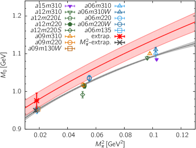
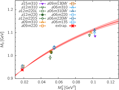
| Fit | /dof | |||||||
|---|---|---|---|---|---|---|---|---|
| [-value] | ||||||||
| 1 | 0.931(22) | -0.273(391) | 0.34(1.96) | 2.722(487) | -2.2(1.3) | -10.9(5.1) | 0.9755(202) | 0.45 [0.87] |
| 2 | 0.430(80) | -3.14(53) | 2.875(48) | -2.6(1.3) | -5.6(4.2) | 0.939 | 0.81 [0.59] |
Appendix C ESC in the extraction of the form factors
In this Appendix, we show the data and the -state fits used to control the ESC in the extraction of the electric and magnetic form factors. There are three sets of figures:
- •
-
•
The improvement in the quality of the signal with increase in the lattice size is shown in Fig. 30 using data from for the three ensembles , and . A study of finite size effects in the form factors using these three ensembles are examined in Fig. 31, and in the extraction of and using the dipole, and fits in Fig. 32.
- •
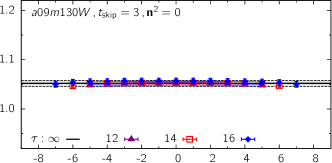
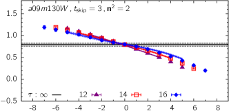
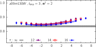
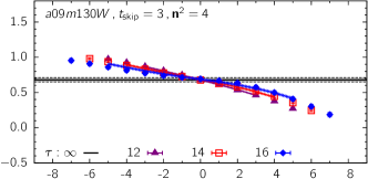
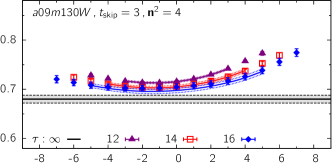
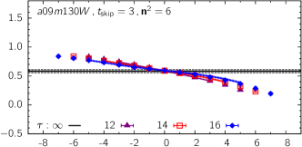
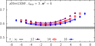
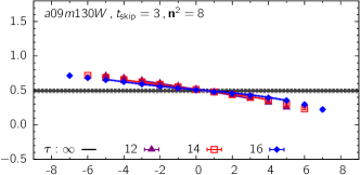
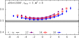
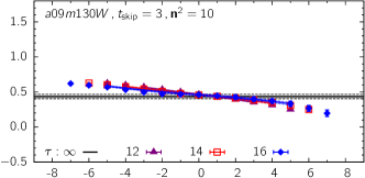
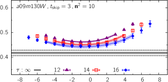
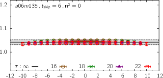
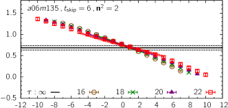
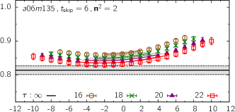
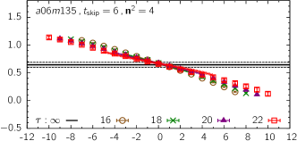
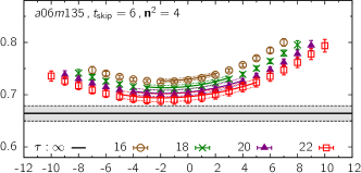
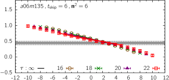
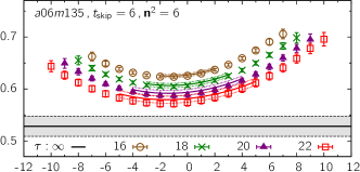
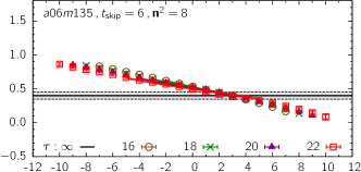
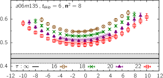
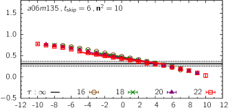
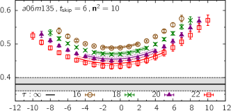
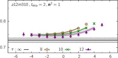
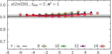
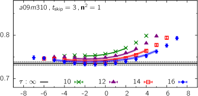
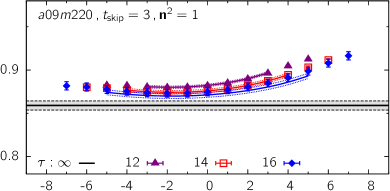
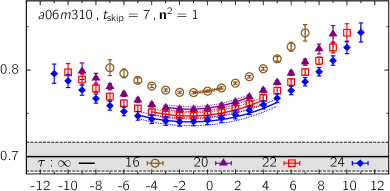
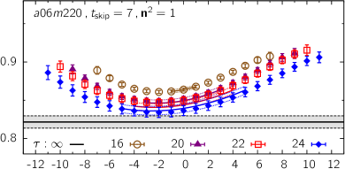
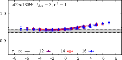
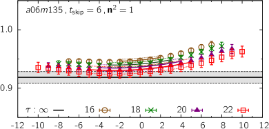
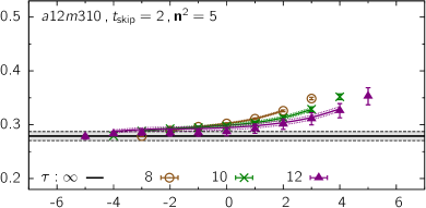
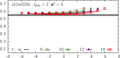
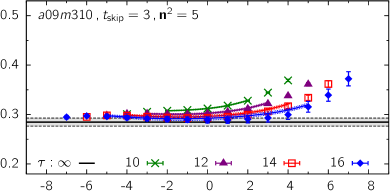
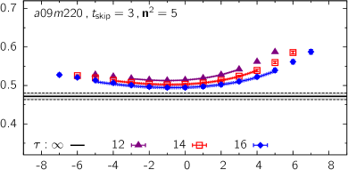
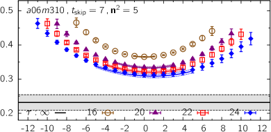
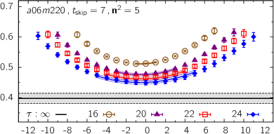
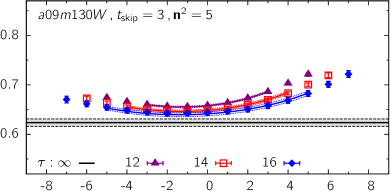
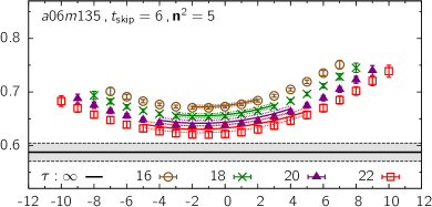
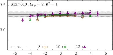
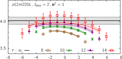
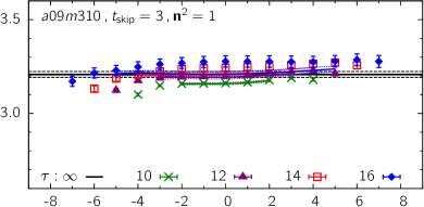
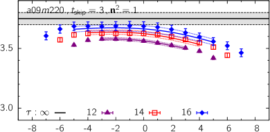
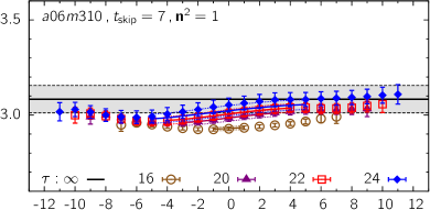
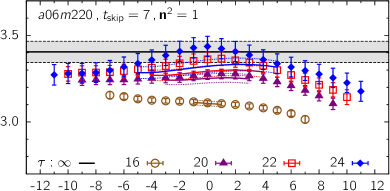
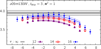
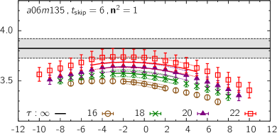
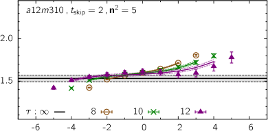
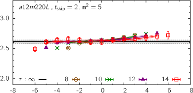
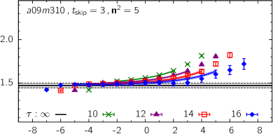
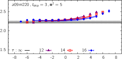
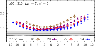
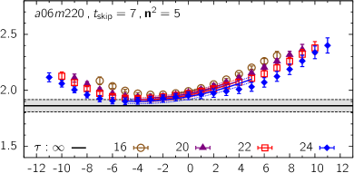
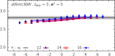
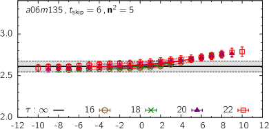
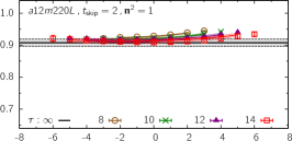
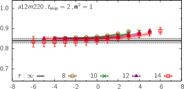
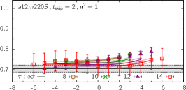
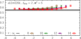
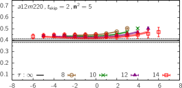
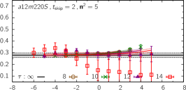
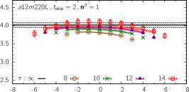
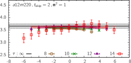
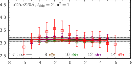
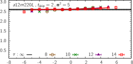
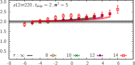
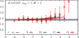
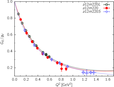
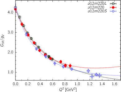
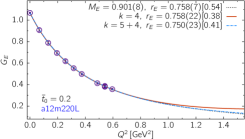
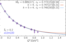
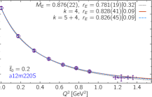
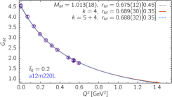
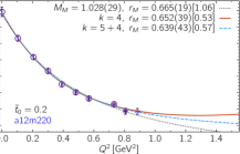
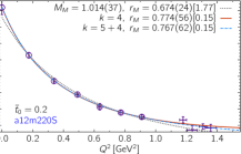
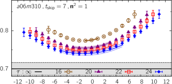
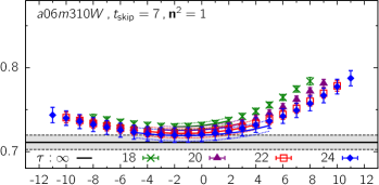
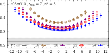
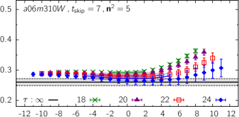
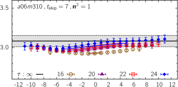
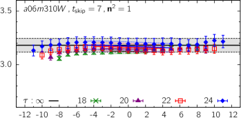

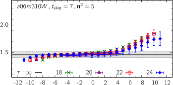
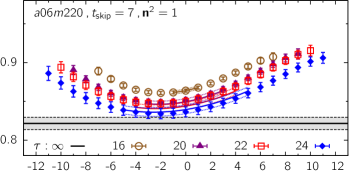
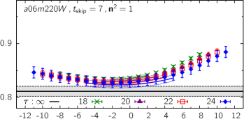
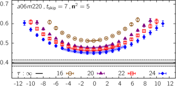
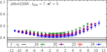
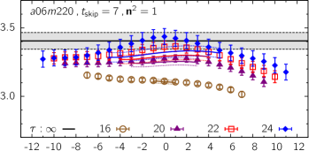
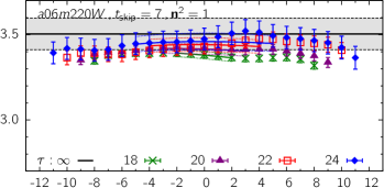
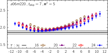
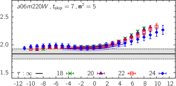
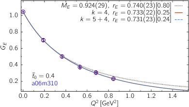
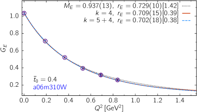
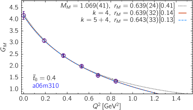
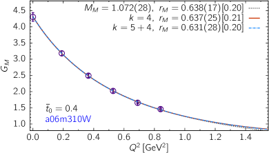
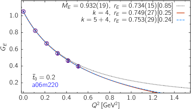
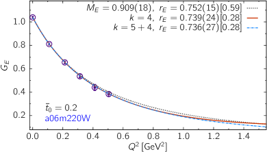
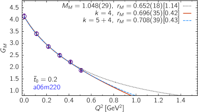
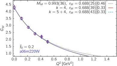
Appendix D Summary of Experimental form factors
In this Appendix, we collect in one place the experimental data for the form factors for the proton and the neutron. In Fig. 36, we show the data for and compiled by Douglas Higinbotham Yan et al. (2018); Alarcón et al. (2019); Higinbotham and McClellan (2019) from the cross sections provided in the Lee-Arlington-Hill supplemental material Lee et al. (2015), who rebinned the original data obtained by the A1 Collaboration using the MAMI beam at Mainz Bernauer et al. (2010, 2014). The neutron data, , are collected from Refs. Gentile and Crawford (2011); Schiavilla and Sick (2001); Sulkosky et al. (2017), and from Refs. Anderson et al. (2007); Anklin et al. (1994, 1998); Bartel et al. (1973, 1972); Bermuth et al. (2003); Bruins et al. (1995); Budnitz et al. (1968); Eden et al. (1994); Esaulov et al. (1987); Gao et al. (1994); Golak et al. (2001); Glazier et al. (2005); Hanson et al. (1973); Herberg et al. (1999); Kubon et al. (2002); Madey et al. (2003); Markowitz et al. (1993); Meyerhoff et al. (1994); Ostrick et al. (1999); Passchier et al. (1999); Plaster et al. (2006); Rohe et al. (1999); Stein et al. (1966); Warren et al. (2004); Zhu et al. (2001). These are shown in Fig. 37. From these data, we evaluate the isovector form factors and to which our lattice data are compared.
The construction of the isovector form factors is done as follows: we first fit the four sets of experimental data for GeV2 using the Kelly parameterization as shown in Figs. 36 and 37. Using the resulting Kelly fits, we then construct the isovector combinations, and . This parameterization is used throughout the paper to compare the lattice data against. From this procedure we get
| (30) |
whereas, using the parameter values given in the original Kelly fit Kelly (2004) gives
| (31) |
Lattice results for the isovector combination of the radii should be compared to the values given in Eq. (30). Note that our less sophisticated analysis, which is also used to analyze the lattice data, gives larger errors.
The results of the dipole fits to the proton data shown in Fig. 36 give and , which are roughly consistent with the careful analysis of electron-experiment results Yan et al. (2018) given in Eqs. (13) and (14) and the Kelly fits shown in the bottom row of Fig. 36. Overall, the dipole ansatz does a good job of fitting the experimental data, and the deviation is less than 1% for GeV2. The dipole fit to is less good as shown by the large .
The convergence of the -expansion fits, with constraints on the , versus is shown in Fig. 38. Estimates with are stable for all three quantities.The results from -expansion fits, also shown in Fig. 36, are marginally larger than those from the dipole and differ by a few percent from those in Eqs. (13) and (14). The errors in the -expansion estimates are larger, especially with the inclusion of the sum rules. The overall lesson from this exercise is that an uncertainty of could be present in our analysis using either the dipole or the -expansion fits.
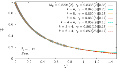
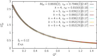
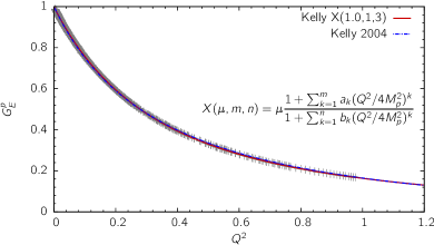
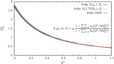
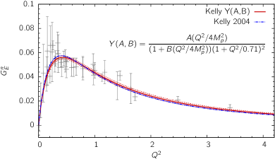
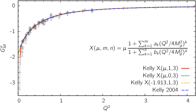
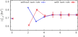
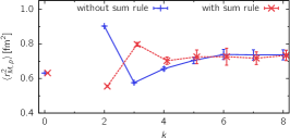
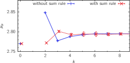
Acknowledgements.
We thank the MILC Collaboration for providing the 2+1+1-flavor HISQ lattices used in our calculations. The calculations used the Chroma software suite Edwards and Joo (2005). R. Gupta thanks D. Higinbotham for discussions and for providing the experimental data on the form factors. Simulations were carried out on computer facilities of (i) the National Energy Research Scientific Computing Center, a DOE Office of Science User Facility supported by the Office of Science of the U.S. Department of Energy under Contract No. DE-AC02-05CH11231; and, (ii) the Oak Ridge Leadership Computing Facility at the Oak Ridge National Laboratory, which is supported by the Office of Science of the U.S. Department of Energy under Contract No. DE-AC05-00OR22725; (iii) the USQCD Collaboration, which are funded by the Office of Science of the U.S. Department of Energy, and (iv) Institutional Computing at Los Alamos National Laboratory. T. Bhattacharya and R. Gupta were partly supported by the U.S. Department of Energy, Office of Science, Office of High Energy Physics under Contract No. DE-AC52-06NA25396. T. Bhattacharya, R. Gupta, J.-C. Jang and B.Yoon were partly supported by the LANL LDRD program. The work of H.-W. Lin is supported by the US National Science Foundation under grant PHY 1653405 “CAREER: Constraining Parton Distribution Functions for New-Physics Searches”.References
- Perdrisat et al. (2007) C. F. Perdrisat, V. Punjabi, and M. Vanderhaeghen, Prog. Part. Nucl. Phys. 59, 694 (2007), arXiv:hep-ph/0612014 [hep-ph] .
- Punjabi et al. (2005) V. Punjabi et al., Phys. Rev. C71, 055202 (2005), [Erratum: Phys. Rev.C71,069902(2005)], arXiv:nucl-ex/0501018 [nucl-ex] .
- Bernauer et al. (2014) J. C. Bernauer et al. (A1), Phys. Rev. C90, 015206 (2014), arXiv:1307.6227 [nucl-ex] .
- Mohr et al. (2016) P. J. Mohr, D. B. Newell, and B. N. Taylor, Rev. Mod. Phys. 88, 035009 (2016), arXiv:1507.07956 [physics.atom-ph] .
- Antognini et al. (2013) A. Antognini et al., Science 339, 417 (2013).
- Antognini et al. (2016) A. Antognini et al., Proceedings, 21st International Conference on Few-Body Problems in Physics (FB21): Chicago, IL, USA, May 18-22, 2015, EPJ Web Conf. 113, 01006 (2016), arXiv:1509.03235 [physics.atom-ph] .
- Ye et al. (2018) Z. Ye, J. Arrington, R. J. Hill, and G. Lee, Phys. Lett. B777, 8 (2018), arXiv:1707.09063 [nucl-ex] .
- Gayou et al. (2002) O. Gayou et al. (Jefferson Lab Hall A), Phys. Rev. Lett. 88, 092301 (2002), arXiv:nucl-ex/0111010 [nucl-ex] .
- Electro-Magnetic Form Factor collaboration, Jefferson Lab() (EMFF) Electro-Magnetic Form Factor (EMFF) collaboration, Jefferson Lab, “Existing measurements and expected statistical accuracy for the GEp experiment,” .
- Bhattacharya et al. (2014) T. Bhattacharya, S. D. Cohen, R. Gupta, A. Joseph, H.-W. Lin, et al., Phys.Rev. D89, 094502 (2014), arXiv:1306.5435 [hep-lat] .
- Green et al. (2014) J. R. Green, J. W. Negele, A. V. Pochinsky, S. N. Syritsyn, M. Engelhardt, and S. Krieg, Phys. Rev. D90, 074507 (2014), arXiv:1404.4029 [hep-lat] .
- Capitani et al. (2015) S. Capitani, M. Della Morte, D. Djukanovic, G. von Hippel, J. Hua, B. Jäger, B. Knippschild, H. B. Meyer, T. D. Rae, and H. Wittig, Phys. Rev. D92, 054511 (2015), arXiv:1504.04628 [hep-lat] .
- Alexandrou et al. (2017a) C. Alexandrou, M. Constantinou, K. Hadjiyiannakou, K. Jansen, C. Kallidonis, G. Koutsou, K. Ottnad, and A. Vaquero, in Proceedings, 34th International Symposium on Lattice Field Theory (Lattice 2016): Southampton, UK, July 24-30, 2016 (2017) arXiv:1702.00984 [hep-lat] .
- Follana et al. (2007) E. Follana et al. (HPQCD Collaboration, UKQCD Collaboration), Phys.Rev. D75, 054502 (2007), arXiv:hep-lat/0610092 [hep-lat] .
- Bazavov et al. (2013) A. Bazavov et al. (MILC Collaboration), Phys.Rev. D87, 054505 (2013), arXiv:1212.4768 [hep-lat] .
- Kelly (2004) J. J. Kelly, Phys. Rev. C70, 068202 (2004).
- Patrignani et al. (2016) C. Patrignani et al. (Particle Data Group), Chin. Phys. C40, 100001 (2016).
- Miller (2019) G. A. Miller, Phys. Rev. C99, 035202 (2019), arXiv:1812.02714 [nucl-th] .
- Gupta et al. (2018) R. Gupta, Y.-C. Jang, B. Yoon, H.-W. Lin, V. Cirigliano, and T. Bhattacharya, Phys. Rev. D98, 034503 (2018), arXiv:1806.09006 [hep-lat] .
- Krauth et al. (2017) J. J. Krauth et al., in Proceedings, 52nd Rencontres de Moriond on Electroweak Interactions and Unified Theories: La Thuile, Italy, March 18-25, 2017 (2017) pp. 95–102, arXiv:1706.00696 [physics.atom-ph] .
- Pohl et al. (2017) R. Pohl et al., Metrologia 54, L1 (2017), arXiv:1607.03165 [physics.atom-ph] .
- Sick and Trautmann (2014) I. Sick and D. Trautmann, Phys. Rev. C89, 012201 (2014), arXiv:1407.1676 [nucl-ex] .
- Sick and Trautmann (2017) I. Sick and D. Trautmann, Phys. Rev. C95, 012501 (2017), arXiv:1701.01809 [nucl-ex] .
- Tanabashi et al. (2018) M. Tanabashi et al. (Particle Data Group), Phys. Rev. D98, 030001 (2018).
- (25) CODATA-2018, “Proton rms charge radius,” .
- Weber et al. (2016) A. Weber, M. Mihovilovic, and H. Merkel (A1), Proceedings, 54th International Winter Meeting on Nuclear Physics (Bormio 2016): Bormio, Italy, January 25-29, 2016, PoS BORMIO2016, 001 (2016).
- Gasparian (2017) A. H. Gasparian (PRad), Proceedings, 14th International Conference on Meson-Nucleon Physics and the Structure of the Nucleon (MENU 2016): Kyoto, Japan, July 25-30, 2016, JPS Conf. Proc. 13, 020052 (2017).
- Lepage and Brodsky (1980) G. P. Lepage and S. J. Brodsky, Phys. Rev. D22, 2157 (1980).
- Hill and Paz (2010) R. J. Hill and G. Paz, Phys. Rev. D82, 113005 (2010), arXiv:1008.4619 [hep-ph] .
- Bhattacharya et al. (2011) B. Bhattacharya, R. J. Hill, and G. Paz, Phys. Rev. D84, 073006 (2011), arXiv:1108.0423 [hep-ph] .
- Lee et al. (2015) G. Lee, J. R. Arrington, and R. J. Hill, Proceedings, Meeting of the APS Division of Particles and Fields (DPF 2015): Ann Arbor, Michigan, USA, 4-8 Aug 2015, Phys. Rev. D92, 013013 (2015), arXiv:1505.01489 [hep-ph] .
- Babich et al. (2010) R. Babich, J. Brannick, R. Brower, M. Clark, T. Manteuffel, et al., Phys.Rev.Lett. 105, 201602 (2010), arXiv:1005.3043 [hep-lat] .
- Bhattacharya et al. (2016) T. Bhattacharya, V. Cirigliano, S. Cohen, R. Gupta, H.-W. Lin, and B. Yoon, Phys. Rev. D94, 054508 (2016), arXiv:1606.07049 [hep-lat] .
- Gupta et al. (2017) R. Gupta, Y.-C. Jang, H.-W. Lin, B. Yoon, and T. Bhattacharya, Phys. Rev. D96, 114503 (2017), arXiv:1705.06834 [hep-lat] .
- Bali et al. (2010) G. S. Bali, S. Collins, and A. Schafer, Comput.Phys.Commun. 181, 1570 (2010), arXiv:0910.3970 [hep-lat] .
- Blum et al. (2013) T. Blum, T. Izubuchi, and E. Shintani, Phys.Rev. D88, 094503 (2013), arXiv:1208.4349 [hep-lat] .
- Bratt et al. (2010) J. Bratt et al. (LHPC Collaboration), Phys.Rev. D82, 094502 (2010), arXiv:1001.3620 [hep-lat] .
- Yoon et al. (2016) B. Yoon et al., Phys. Rev. D93, 114506 (2016), arXiv:1602.07737 [hep-lat] .
- Güsken et al. (1989) S. Güsken, U. Löw, K. H. Mütter, R. Sommer, A. Patel, and K. Schilling, Phys. Lett. B227, 266 (1989).
- Bhattacharya et al. (2015) T. Bhattacharya, V. Cirigliano, S. Cohen, R. Gupta, A. Joseph, H.-W. Lin, and B. Yoon (PNDME), Phys. Rev. D92, 094511 (2015), arXiv:1506.06411 [hep-lat] .
- Yoon et al. (2017) B. Yoon et al., Phys. Rev. D95, 074508 (2017), arXiv:1611.07452 [hep-lat] .
- Sommer (2014) R. Sommer, Proceedings, 31st International Symposium on Lattice Field Theory (Lattice 2013): Mainz, Germany, July 29-August 3, 2013, PoS LATTICE2013, 015 (2014), arXiv:1401.3270 [hep-lat] .
- Yan et al. (2018) X. Yan, D. W. Higinbotham, D. Dutta, H. Gao, A. Gasparian, M. A. Khandaker, N. Liyanage, E. Pasyuk, C. Peng, and W. Xiong, Phys. Rev. C98, 025204 (2018), arXiv:1803.01629 [nucl-ex] .
- Punjabi and Perdrisat (2014) V. Punjabi and C. F. Perdrisat, Proceedings, 25th International Nuclear Physics Conference (INPC 2013): Florence, Italy, June 2-7, 2013, EPJ Web Conf. 66, 06019 (2014), arXiv:1403.5504 [nucl-ex] .
- Kubis and Meissner (2001) B. Kubis and U.-G. Meissner, Nucl. Phys. A679, 698 (2001), arXiv:hep-ph/0007056 [hep-ph] .
- Bernard et al. (1998) V. Bernard, H. W. Fearing, T. R. Hemmert, and U. G. Meissner, Nucl. Phys. A635, 121 (1998), [Erratum: Nucl. Phys.A642,563(1998)], arXiv:hep-ph/9801297 [hep-ph] .
- Gockeler et al. (2005) M. Gockeler, T. R. Hemmert, R. Horsley, D. Pleiter, P. E. L. Rakow, A. Schafer, and G. Schierholz (QCDSF), Phys. Rev. D71, 034508 (2005), arXiv:hep-lat/0303019 [hep-lat] .
- Beane (2004) S. R. Beane, Phys. Rev. D70, 034507 (2004), arXiv:hep-lat/0403015 [hep-lat] .
- Beane and Savage (2003) S. R. Beane and M. J. Savage, Phys. Rev. D68, 114502 (2003), arXiv:hep-lat/0306036 [hep-lat] .
- de Divitiis et al. (2004) G. M. de Divitiis, R. Petronzio, and N. Tantalo, Phys. Lett. B595, 408 (2004), arXiv:hep-lat/0405002 [hep-lat] .
- [ALPHA 01] R. Frezzotti et al. (2001) [ALPHA 01] R. Frezzotti, P. A. Grassi, S. Sint, and P. Weisz, JHEP 08, 058 (2001), arXiv:hep-lat/0101001 .
- Green et al. (2015) J. Green, S. Meinel, M. Engelhardt, S. Krieg, J. Laeuchli, J. Negele, K. Orginos, A. Pochinsky, and S. Syritsyn, Phys. Rev. D92, 031501 (2015), arXiv:1505.01803 [hep-lat] .
- Alexandrou et al. (2017b) C. Alexandrou, M. Constantinou, K. Hadjiyiannakou, K. Jansen, C. Kallidonis, G. Koutsou, and A. Vaquero Aviles-Casco, Phys. Rev. D96, 034503 (2017b), arXiv:1706.00469 [hep-lat] .
- Hasan et al. (2018) N. Hasan, J. Green, S. Meinel, M. Engelhardt, S. Krieg, J. Negele, A. Pochinsky, and S. Syritsyn, Phys. Rev. D97, 034504 (2018), arXiv:1711.11385 [hep-lat] .
- Ishikawa et al. (2018) K.-I. Ishikawa, Y. Kuramashi, S. Sasaki, N. Tsukamoto, A. Ukawa, and T. Yamazaki (PACS), Phys. Rev. D98, 074510 (2018), arXiv:1807.03974 [hep-lat] .
- Shintani et al. (2019) E. Shintani, K.-I. Ishikawa, Y. Kuramashi, S. Sasaki, and T. Yamazaki, Phys. Rev. D99, 014510 (2019), arXiv:1811.07292 [hep-lat] .
- Alexandrou et al. (2018) C. Alexandrou, S. Bacchio, M. Constantinou, J. Finkenrath, K. Hadjiyiannakou, K. Jansen, G. Koutsou, and A. V. A. Casco, (2018), arXiv:1812.10311 [hep-lat] .
- Hasan et al. (2019) N. Hasan, J. Green, S. Meinel, M. Engelhardt, S. Krieg, J. Negele, A. Pochinsky, and S. Syritsyn, (2019), arXiv:1903.06487 [hep-lat] .
- Ishikawa et al. (2016) K. I. Ishikawa, N. Ishizuka, Y. Kuramashi, Y. Nakamura, Y. Namekawa, Y. Taniguchi, N. Ukita, T. Yamazaki, and T. Yoshie (PACS), Proceedings, 33rd International Symposium on Lattice Field Theory (Lattice 2015): Kobe, Japan, July 14-18, 2015, PoS LATTICE2015, 075 (2016), arXiv:1511.09222 [hep-lat] .
- Edwards and Joo (2005) R. G. Edwards and B. Joo (SciDAC Collaboration, LHPC Collaboration, UKQCD Collaboration), Nucl.Phys.Proc.Suppl. 140, 832 (2005), arXiv:hep-lat/0409003 [hep-lat] .
- Alarcón et al. (2019) J. M. Alarcón, D. W. Higinbotham, C. Weiss, and Z. Ye, Phys. Rev. C99, 044303 (2019), arXiv:1809.06373 [hep-ph] .
- Higinbotham and McClellan (2019) D. W. Higinbotham and R. E. McClellan, (2019), arXiv:1902.08185 [physics.data-an] .
- Bernauer et al. (2010) J. C. Bernauer et al. (A1), Phys. Rev. Lett. 105, 242001 (2010), arXiv:1007.5076 [nucl-ex] .
- Gentile and Crawford (2011) T. R. Gentile and C. B. Crawford, Phys. Rev. C83, 055203 (2011).
- Schiavilla and Sick (2001) R. Schiavilla and I. Sick, Phys. Rev. C64, 041002 (2001), arXiv:nucl-ex/0107004 [nucl-ex] .
- Sulkosky et al. (2017) V. Sulkosky et al., Phys. Rev. C96, 065206 (2017), arXiv:1704.06253 [nucl-ex] .
- Anderson et al. (2007) B. Anderson et al. (Jefferson Lab E95-001), Phys. Rev. C75, 034003 (2007), arXiv:nucl-ex/0605006 [nucl-ex] .
- Anklin et al. (1994) H. Anklin et al., Phys. Lett. B336, 313 (1994).
- Anklin et al. (1998) H. Anklin et al., Phys. Lett. B428, 248 (1998).
- Bartel et al. (1973) W. Bartel, F. W. Busser, W. r. Dix, R. Felst, D. Harms, H. Krehbiel, P. E. Kuhlmann, J. McElroy, J. Meyer, and G. Weber, Nucl. Phys. B58, 429 (1973).
- Bartel et al. (1972) W. Bartel, F. W. Buesser, W. R. Dix, R. Felst, D. Harms, H. Krehbiel, P. E. Kuhlmann, J. Mcelroy, J. Meyer, and G. Weber, Phys. Lett. 39B, 407 (1972).
- Bermuth et al. (2003) J. Bermuth et al., Phys. Lett. B564, 199 (2003), arXiv:nucl-ex/0303015 [nucl-ex] .
- Bruins et al. (1995) E. E. W. Bruins et al., Phys. Rev. Lett. 75, 21 (1995).
- Budnitz et al. (1968) R. J. Budnitz et al., Phys. Rev. 173, 1357 (1968).
- Eden et al. (1994) T. Eden et al., Phys. Rev. C50, R1749 (1994).
- Esaulov et al. (1987) A. S. Esaulov, A. P. Rekalo, M. P. Rekalo, Yu. I. Titov, R. V. Akhmerov, and E. M. Smelov, Sov. J. Nucl. Phys. 45, 258 (1987), [Yad. Fiz.45,410(1987)].
- Gao et al. (1994) H. Gao et al., Phys. Rev. C50, R546 (1994).
- Golak et al. (2001) J. Golak, G. Ziemer, H. Kamada, H. Witala, and W. Gloeckle, Phys. Rev. C63, 034006 (2001), arXiv:nucl-th/0008008 [nucl-th] .
- Glazier et al. (2005) D. I. Glazier et al., Eur. Phys. J. A24, 101 (2005), arXiv:nucl-ex/0410026 [nucl-ex] .
- Hanson et al. (1973) K. M. Hanson, J. R. Dunning, M. Goitein, T. Kirk, L. E. Price, and R. Wilson, Phys. Rev. D8, 753 (1973).
- Herberg et al. (1999) C. Herberg et al., Eur. Phys. J. A5, 131 (1999).
- Kubon et al. (2002) G. Kubon et al., Phys. Lett. B524, 26 (2002), arXiv:nucl-ex/0107016 [nucl-ex] .
- Madey et al. (2003) R. Madey et al. (E93-038), Phys. Rev. Lett. 91, 122002 (2003), arXiv:nucl-ex/0308007 [nucl-ex] .
- Markowitz et al. (1993) P. Markowitz et al., Phys. Rev. C48, R5 (1993).
- Meyerhoff et al. (1994) M. Meyerhoff et al., Phys. Lett. B327, 201 (1994).
- Ostrick et al. (1999) M. Ostrick et al., Phys. Rev. Lett. 83, 276 (1999).
- Passchier et al. (1999) I. Passchier et al., Phys. Rev. Lett. 82, 4988 (1999), arXiv:nucl-ex/9907012 [nucl-ex] .
- Plaster et al. (2006) B. Plaster et al. (Jefferson Laboratory E93-038), Phys. Rev. C73, 025205 (2006), arXiv:nucl-ex/0511025 [nucl-ex] .
- Rohe et al. (1999) D. Rohe et al., Phys. Rev. Lett. 83, 4257 (1999).
- Stein et al. (1966) P. Stein, M. Binkley, R. McAllister, A. Suri, and W. Woodward, Phys. Rev. Lett. 16, 592 (1966).
- Warren et al. (2004) G. Warren et al. (Jefferson Lab E93-026), Phys. Rev. Lett. 92, 042301 (2004), arXiv:nucl-ex/0308021 [nucl-ex] .
- Zhu et al. (2001) H. Zhu et al. (E93026), Phys. Rev. Lett. 87, 081801 (2001), arXiv:nucl-ex/0105001 [nucl-ex] .