(f)RFCDE: Random Forests for Conditional Density Estimation and Functional Data

Abstract

Random forests is a common non-parametric regression technique which performs well for mixed-type unordered data and irrelevant features, while being robust to monotonic variable transformations. Standard random forests, however, do not efficiently handle functional data and runs into a curse-of-dimensionality when presented with high-resolution curves and surfaces. Furthermore, in settings with heteroskedasticity or multimodality, a regression point estimate with standard errors do not fully capture the uncertainty in our predictions. A more informative quantity is the conditional density $p(y\mid x)$ which describes the full extent of the uncertainty in the response $y$ given covariates $x$. In this paper we show how random forests can be efficiently leveraged for conditional density estimation, functional covariates, and multiple responses without increasing computational complexity. We provide open-source software for all procedures with R and Python versions that call a common C++ library.

1 Introduction and Motivation

Conditional density estimation (CDE) is the estimation of the density $p(y\mid x)$ where we condition the response $y$ on observed covariates $x$. In a prediction context, CDE provides a more nuanced accounting of uncertainty than a point estimate or prediction interval, especially in the presence of heteroskedastic or multimodal responses. Conditional density estimation has proven useful in a range of applications; e.g., econometrics [Li and Racine, 2007], astronomy [Group, ] and likelihood-free inference [Izbicki et al., 2018].

We extend random forests [Breiman, 2001] to the more challenging problem of CDE, while inheriting the benefits of random forests with respect to interpretability, mixed-data types, feature selection, and data transformations. We take advantage of the fact that random forests can be viewed as a form of adaptive nearest-neighbor method with the aggregated tree structures determining a weighting scheme. This weighting scheme can then be used to estimate quantities other than the conditional mean; in this case the entire conditional density. As shown in Section 3.4, random forests can also be adapted to take the functional nature of curves into account by splitting in the domain of the curves.

Other existing random forest implementations such as quantileregressionForests [Meinshausen, 2006] and trtf [Hothorn and Zeileis, 2017] can be used for CDE. However, the first procedure does not alter the splits of the tree, and the second implementation does not scale to large sample sizes. Neither method handles functional covariates and multiple responses. In Section 3 we show that our method achieves lower CDE loss in competitive computational time for several examples.

In brief, the main contributions of this paper are

1. Our trees are optimized to minimize a conditional density estimation loss while remaining computationally efficient; hence overcoming the limitations of the usual regression approach due to heteroskedasticity and multimodality.

2. We provide new procedures and public software (R and Python wrappers to a common C++ library) for joint conditional density estimation and functional data; this opens the door for interpretable models and uncertainty quantification for a range of modern applications involving different types of complex data from multiple sources.

2 Method

To construct our base conditional density estimator we follow the usual random forest construction with a key modification in the loss function, while retaining algorithms with linear complexity. Here we describe our base algorithm; the extension to functional covariates is described in Section 3.4.

At their simplest, random forests are ensembles of regression trees. Each tree is trained on a bootstrapped sample of the data. The training process involves recursively partitioning the feature space through splitting rules taking the form of splitting into the sets $\left\{X_{i}\leq v\right\}$ and $\left\{X_{i}>v\right\}$ for a particular feature $X_{i}$ and split point $v$. Once a partition becomes small enough (controlled by a tuning parameter), it becomes a leaf node and is no longer partitioned.

For prediction we use the tree structure to calculate weights for the training data from which we perform a weighted kernel density estimate using “nearby” points. This is analogous to the regression case which would perform a weighted mean.

Borrowing the notation of Breiman [2001] and Meinshausen [2006], let $\theta_{t}$ denote the tree structure for a single tree. Let $R(x,\theta_{t})$ denote the region of feature space covered by the leaf node for input $x$. Then for a new observation $x^{*}$ we use $t$-th tree to calculate weights for each training point $x_{i}$ as

$$w_{i}(x^{*},\theta_{t})=\frac{\mathbbm{1}\left[X_{i}\in R(x^{*},\theta_{t})\right]}{\sum_{i=1}^{n}\mathbbm{1}\left[X_{i}\in R(x^{*},\theta_{t})\right]}.$$

We then aggregate over trees, setting $w_{i}(x^{*})=T^{-1}\sum_{t=1}^{T}w_{i}(x^{*},\theta_{t})$. The weights are finally used for the weighted kernel density estimate

$$\widehat{p}(y\mid x^{*})=\frac{1}{\sum_{i=1}^{n}w_{i}(x^{*})}\sum_{i=1}^{n}w_{i}(x^{*})K_{h}(Y_{i}-y)$$ (1)

where $K_{h}$ is a kernel function integrating to one. The bandwidth can be selected using plug-in methods or through tuning based upon a validation set. Up to this point we have the same approach as Meinshausen [2006].

Our departure from the standard random forest algorithm is the criterion for choosing the splits of the partitioning. In regression contexts, the splitting variable and split point are often chosen to minimize the mean-squared error loss. For CDE, we instead choose splits that minimize a loss specific to CDE [Izbicki and Lee, 2017]

$$L(p,\widehat{p})=\int\int\left(p(y\mid x)-\widehat{p}(y\mid x)\right)^{2}\mathop{}\!\mathrm{d}y\mathop{}\!\mathrm{d}P(x).$$

where $P(x)$ is the marginal distribution of $X$.

This loss is the $L^{2}$ error for density estimation weighted by the marginal density of the covariates. To conveniently estimate this loss we can expand the square and rewrite the loss as

$$L(p,\widehat{p})=\operatorname{\mathbb{E}}_{X}\left[\int\widehat{p}^{2}(y\mid X)\mathop{}\!\mathrm{d}y\right]-2\operatorname{\mathbb{E}}_{X,Y}\left[\widehat{p}(Y\mid X)\right]+C_{p}$$ (2)

with $C_{p}$ as a constant which does not depend on $\widehat{p}$. The first expectation is with respect to the marginal distribution of $X$ and the second with respect to the joint distribution of $X$ and $Y$. We estimate these expectations by their empirical expectation on observed data.

To provide intuition why switching the loss function is desirable: consider the example in Figure 1: we have two stationary distributions separated by a transition point at $x=0.5$: the left is a normal distribution centered at zero and the right is a mixture of two normal distributions centered at 1 and -1. The clear split for a tree is the transition point: however, because the generating distribution’s conditional mean is constant for all $x$ the mean-square-error loss fits to noise and picks a poor split point far from $x=0.5$. The CDE loss on the other hand is minimized at the split point.

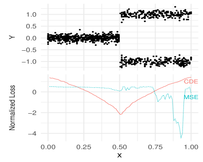
Figure 1: (top) Training data with a switch from a unimodal to bimodal response at x = 0.5; (bottom) the normalized losses for each cut-point. MSE overfits to small differences in the bimodal regime while CDE loss is minimized at the true transition point.

While we use kernel density estimates for predictions on new observations, we do not use kernel density estimates when evaluating splits: the calculations in Equation 2 would be expensive for KDE with the term $\int\widehat{p}(y\mid x)^{2}\mathop{}\!\mathrm{d}y$ depending on the $O(n^{2})$ pairwise distances between all training points.

For fast computations, we instead use orthogonal series to compute density estimates for splitting. Given an orthogonal basis $\left\{\Phi_{j}(y)\right\}$ such as a cosine basis or wavelet basis, we can express the density as $\widehat{p}(y\mid x)=\sum_{j}\widehat{\beta_{j}}\phi_{j}(y)$ where $\widehat{\beta_{j}}=\frac{1}{n}\sum_{i=1}^{n}\phi_{j}(y_{i})$. This choice is motivated by a convenient formula for the CDE loss associated with an orthogonal series density estimate

$$\widehat{L}(p,\widehat{p})-C_{p}=-\sum_{j}\widehat{\beta_{j}}^{2}.$$

The above expression only depends upon the quantities $\left\{\widehat{\beta_{j}}\right\}$ that themselves depend only upon linear sums of $\phi_{j}(y_{i})$. This makes it computationally efficient to evaluate the CDE loss for each split.

3 Results

3.1 Synthetic Experiment

To illustrate the potential benefits of optimizing with respect to a CDE loss, we here compare against an existing random forest quantile method that minimizes an MSE loss. More specifically, we adapt the quantregForest [Meinshausen, 2006] package in R to perform conditional density estimation according to Equation 1. This would then be equivalent to our method except that the splits for quantregForest minimize mean-squared error rather than CDE loss; thereby providing us a means for specifically studying the effect of training random forests for CDE. We also compare against the trtf package [Hothorn and Zeileis, 2017] which trains forests for CDE using flexible parametric families.

We generate data from the following model

$$X_{1:10},Z_{1:10}\sim\operatorname{Uniform}(0,1),\quad S\sim\operatorname{Multinomial}(2,\frac{1}{2})$$

$$Y\mid X,Z,S\sim\begin{cases}\operatorname{Normal}(\left\lfloor\sum_{i}X_{i}\right\rfloor,\sigma)&S=1\\ \operatorname{Normal}(-\left\lfloor\sum_{i}X_{i}\right\rfloor,\sigma)&S=2\\ \end{cases}$$

where the $X_{i}$ are the relevant features with the $Z_{i}$ serving as irrelevant features. $S$ is an unobserved feature which induces multimodality in the conditional densities.

Under the true model $\operatorname{\mathbb{E}}[Y\mid X,Z]=0$, so there is no partitioning scheme that can reduce the MSE loss (as the conditional mean is always zero). As such, the trained quantregForest trees behave similarly to nearest neighbors as splits are effectively chosen at random. We evaluate the three methods on two criterion: training time and CDE loss on a validation set. All models are tuned with the same forest parameters (mtry = 4, ntrees = 1000). RFCDE has n_basis = 15. trtf is fit using a Bernstein basis of order 5. RFCDE and quantregForest have bandwidth 0.2.

Table 1: Performance of RFCDE and competing methods on synthetic data; smaller CDE loss implies better estimates.

Method	N	CDE Loss (SE)	Train Time (seconds)	Predict Time (seconds)
RFCDE	1,000	-0.171 (0.004)	2.31	1.29
quantregForest	1,000	-0.152 (0.003)	1.17	0.61
trtf	1,000	-0.109 (0.001)	1013.54	123.47
RFCDE	10,000	-0.194 (0.003)	42.99	1.95
quantregForest	10,000	-0.159 (0.003)	48.60	0.47
RFCDE	100,000	-0.227 (0.004)	904.76	8.05
quantregForest	100,000	-0.173 (0.003)	1289.93	0.61

Table 1 summarizes the results for three simulations of size 1000, 10,000, and 100,000 training observations. We use 1,000 observations for the test set and calculate the CDE loss. We see that RFCDE performs substantially better on CDE loss. We also note that RFCDE has competitive training time especially for larger data sets. trtf is only run for the smallest data set due to its high computational cost.

3.2 Photo-z Application

We next illustrate our methods on applications in astronomy.

In order to utilize the statistical information in images of galaxies, we need to estimate how far away they are from the Milky Way. A metric for this distance is a galaxy’s redshift, which is a measure of how much the Universe has expanded since the galaxy emitted its light. For the vast majority of galaxies, estimates of redshift probability density functions are made on the basis of brightness measurements at five wavelengths. This is dubbed photometric redshift estimation, or photo-z. Due to degeneracies the pdfs may exhibit, e.g., multi-modality; thus photo-z presents a natural venue for showing the efficacy ofRFCDE.

We perform a similar CDE methods comparison as for the synthetic example using realistically simulated photo-z data from LSST DESC[Group, ]. We split 100,000 training observations into subsets of size 1,000, 10,000, and 100,000, and evaluate the CDE loss on 10,000 held-out observations. We compare only against quantregForest, dropping trtf again for computational reasons. Both models are tuned with the same random forest parameters (mtry = 3, ntrees = 1000). RFCDE has nbasis = 31. Kernel density bandwidths are selected using plug-in estimates. The covariates are the magnitudes for the six LSST filterbands (ugrizy) together with local differences (u - g, g - r, etc) for a total of 11 covariates.

Table 2: Performance of RFCDE and competing methods for photo-z application; smaller CDE loss implies better estimates.

Method	N	CDE Loss (SE)	Train Time (seconds)	Predict Time (seconds)
RFCDE	1,000	-2.394 (0.033)	2.24	14.53
quantregForest	1,000	-2.309 (0.037)	1.36	9.85
RFCDE	10,000	-4.018 (0.054)	34.98	22.17
quantregForest	10,000	-3.809 (0.057)	40.94	9.54
RFCDE	100,000	-5.356 (0.092 )	823.32	65.91
quantregForest	100,000	-5.064 (0.084)	2678.39	10.46

Table 2 summarizes the results: similarly to the synthetic example we find that RFCDE achieves substantially better CDE loss with competitive computational time.

3.3 Extension to Joint CDE

RFCDE can also target joint conditional density estimation, which allows us to capture dependencies in multivariate responses. This feature is particularly useful for estimating Bayesian posterior distributions in e.g. likelihood free inference Izbicki et al. [2018].

The splitting process extends straightforwardly to the multivariate case through the use of a tensor basis ${p}(y_{1},y_{2},\dots,y_{n}\mid x)=\sum_{i}\sum_{j}\beta_{i,j}(x)\phi_{j}(y_{i})$ which results in the same formula for the CDE loss summed over $\widehat{\beta}_{i,j}^{2}$ instead of $\widehat{\beta}_{j}^{2}$. The density estimation similarly extends through the use of multivariate kernel density estimation in Equation 1. Bandwidth selection can be treated as in the univariate case through either plug-in estimators or tuning.

These extensions allow for multivariate CDE estimation (with a current effective limit of three response variables due to the use of the tensor basis). We showcase this by applying RFCDE to a problem related to weak lensing, the slight perturbation of a galaxy’s appearance due to the bending of light by intervening masses. Statistical estimates of how correlated the perturbations are as a function of angular distance allows one to place constraints on two parameters of the Big Bang model: $\Omega_{M}$, the proportion of the Universe’s mass-energy comprised of mass, and $\sigma_{8}$, which relates to how galaxies have clustered as the Universe has evolved. Specifically, we are interested in inferring the joint distribution of $\Omega_{M}$ and $\sigma_{8}$ given observed weak lensing data.

This problem provides an illustrative case for the need to model joint conditional distributions flexibly. There is a degeneracy curve $\Omega_{M}^{\alpha}\sigma_{8}$ on which the data are indistinguishable. In Figure 2 we see thatRFCDE can capture this curved ridge structure well which leads to better parameter constraints; in the example we used the GalSim toolkit [Rowe et al., 2015] to simulate shear correlation functions under different parameter settings.

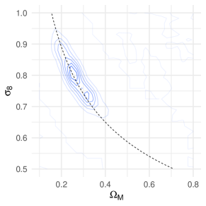
Figure 2: The posterior distribution of the parameters $\Omega_{M}$ and $\sigma_{8}$ exhibits a ridge structure whichRFCDE captures due to splitting on CDE loss for joint densities.

3.4 Extension to Functional Data

Treating functional covariates (like correlation functions or images) as unordered multivariate vectors on a grid suffers from a curse-of-dimensionality: as the resolution of the grid becomes finer you increase the dimensionality of the data but add little additional information due to high correlation between nearby grid points.

To adapt to this setting we follow the approach of Möller et al. [2016] by partitioning the functional covariates of each tree in their domain, and passing the mean values of the function for each partition as inputs to the tree.

The partitioning is governed by the parameter $\lambda$ of a Poisson process; starting at the first element of the function evaluation vector we take the next $\operatorname{Poisson}(\lambda)$ evaluations as one interval in the partition. We then repeat the procedure, starting at the end of that interval and continuing until we have partitioned the entire function domain into disjoint regions $\left\{(l_{i},h_{i})\right\}$. Once we have partitioned the function domain we take the function mean value $\int_{l_{i}}^{h_{i}}f(x)dx$ within each region as the covariates for the random forest.

We illustrate our functional RFCDE method on spectroscopic data for 3,000 galaxies from the Sloan Digital Sky Survey. The functional covariates consist of the observed spectrum of each galaxy at 3,421 different wavelengths; the response is the redshift of the galaxy. These spectra can be viewed as a high-resolution version of the photometric data from Section 3.2.

To show the benefits of taking the functional structure of the data into account, we compare the results of a base version ofRFCDE as described in Section 2 withRFCDE for functional covariates. We set $\lambda$ = 50. Both trees are otherwise trained identically: ntrees = 1000, n_basis = 31, and the bandwidths are chosen using plug-in estimators. We train on 2000 examples and use the remaining 1000 to evaluate the CDE loss.

Table 3: Performance of RFCDE for functional data. We see that we obtain both better CDE loss and computational time by taking advantage of the structure of the functional data.

Method	Train Time (sec)	CDE Loss (SE)
Functional	12.62	-29.623 (0.844)
Vector	21.31	-12.578 (0.418)

Table 3 shows the CDE loss for both the vector-based and functional-based RFCDE models on the SDSS data. We obtain substantial gains with a functional approach both in terms of CDE loss as well as computational time. The computational gains are attributed to requiring fewer searches for each split point as the default value of mtry = sqrt(d) is reduced.

4 Summary

We adapt random forests to conditional density estimation through the introduction of an alternative loss function for selecting splits in the trees of the random forest. This loss function is sensitive to changes in the distribution of responses, which losses based upon regression can miss. We exhibit improved performance and comparable computational speed for a variety of different data examples including functional data and joint conditional distributions. We provide a software package RFCDE for fitting this model consisting of a C++ library with R and Python wrappers. These packages along with documentation are available at https://github.com/tpospisi/rfcde.

References

- Breiman [2001] L. Breiman. Random forests. Machine learning, 45(1):5–32, 2001.
- [2] L.-D. P. R. W. Group. An assessment of photometric redshift pdf performance in the context of lsst. under review.
- Hothorn and Zeileis [2017] T. Hothorn and A. Zeileis. Transformation forests. arXiv:1701.02110, 2017.
- Izbicki and Lee [2017] R. Izbicki and A. B. Lee. Converting high-dimensional regression to high-dimensional conditional density estimation. Electronic Journal of Statistics, 11(2):2800–2831, 2017.
- Izbicki et al. [2018] R. Izbicki, A. B. Lee, and T. Pospisil. Abc-cde: Towards approximate bayesian computation with complex high-dimensional data and limited simulations. arXiv preprint arXiv:1805.05480, 2018.
- Li and Racine [2007] Q. Li and J. S. Racine. Nonparametric econometrics: theory and practice. Princeton University Press, 2007.
- Meinshausen [2006] N. Meinshausen. Quantile regression forests. Journal of Machine Learning Research, 7:983–999, 2006.
- Möller et al. [2016] A. Möller, G. Tutz, and J. Gertheiss. Random forests for functional covariates. Journal of Chemometrics, 30(12):715–725, 2016.
- Rowe et al. [2015] B. Rowe, M. Jarvis, R. Mandelbaum, G. M. Bernstein, J. Bosch, M. Simet, J. E. Meyers, T. Kacprzak, R. Nakajima, J. Zuntz, et al. Galsim: The modular galaxy image simulation toolkit. Astronomy and Computing, 10:121–150, 2015.