Computation of intrinsic spin Hall conductivities from first principles using maximally-localized Wannier functions

Abstract

We present a method to compute the intrinsic spin Hall conductivity from first principles using an interpolation scheme based on maximally-localized Wannier functions. After obtaining the relevant matrix elements among the ab initio Bloch states calculated on a coarse $k$-point mesh, we Fourier transform them to find the corresponding matrix elements between Wannier states. We then perform an inverse Fourier transform to interpolate the velocity and spin-current matrix elements onto a dense $k$-point mesh, and use them to evaluate the spin Hall conductivity as a Brillouin-zone integral. This strategy has a much lower computational cost than a direct ab initio calculation, without sacrificing the accuracy. We demonstrate that the spin Hall conductivities of platinum and doped gallium arsenide, computed with our interpolation scheme as a function of the Fermi energy, are in good agreement with those obtained in previous first-principles studies. We also discuss certain approximations that can be made, in the spirit of the tight-binding method, to simplify the calculation of the velocity and spin-current matrix elements in the Wannier representation.

I introduction

The spin Hall effect is a phenomenon in which a transverse spin current is generated in response to a bias voltage. Sinova et al. (2015); Sinova and Žutić (2012); Jungwirth et al. (2012) Together with its inverse effect,Hirsch (1999); Saitoh et al. (2006) the conversion of charge current into spin current by the spin Hall effect has been used to electrically inject or detect spin,Kimura et al. (2007) to fabricate spin field-effect transistors,Wunderlich et al. (2010) to manipulate spin dynamics in magnetic microstructures,Ando et al. (2008) and to exert significant spin torques in an adjacent magnetic film.Liu et al. (2011, 2012) In order to utilize the spin Hall effect, it is desirable to find materials with large spin Hall conductivities (SHCs).

In the weak-disorder limit, the SHC of conducting systems such as metals and doped semiconductors is usually divided into three contributions:Nagaosa et al. (2010); Sinova et al. (2015) (i) the skew-scattering contribution, which is inversely proportional to the concentration of impurities; (ii) the intrinsic contribution, which is independent of the concentration of impurities and whose value is fully determined by the electronic properties of the pristine material; and (iii) the side-jump contribution, which is independent of the concentration of impurities but whose value depends on the details of the disorder potential.

Contrary to the intrinsic contribution, the other two contributions depend on disorder, which is why they are considered extrinsic. Calculations of the extrinsic contributions to the SHC have been mostly limited to simple toy-model systems such as two-dimensional electron Inoue et al. (2004) or hole Bernevig and Zhang (2005) gases. More recently, a first-principles methodology for calculating those contributions has been developed.Chadova et al. (2015) It has been reported that in many materials with strong spin-orbit coupling the intrinsic contribution accounts for a significant portion of the SHC (see, for example, Ref. Guo et al., 2008; for more details, see Ref. Nagaosa et al., 2010; Sinova et al., 2015 and references therein). For this reason, most first-principles studies of the spin Hall effect in conducting systems have focused exclusively on the intrinsic contribution.

The intrinsic SHC can be calculated from the Kubo formula given in Eq. (1) below. The needed ingredients are the Bloch eigenstates and energy eigenvalues of the pristine crystal, which are typically obtained from a first-principles calculation based on density-functional theory. Such calculations were initially performed for simple semiconductors Guo et al. (2005) and metals,Guo et al. (2008); Guo (2009) and recently they have been carried out for more complex systems such as metallic alloys.Sui et al. (2017) Those studies revealed that a rather dense $k$-point mesh is often needed to converge the calculation. This happens when, in some regions of the Brillouin zone (BZ), occupied and empty states are both present close to the Fermi level, leading to a resonant enhancement of the energy denominator in Eq. (1). Calculating the needed Bloch states directly from first principles over a large number of $k$ points is very demanding, and it would be desirable to develop more efficient algorithms.

In this work, we present a method that circumvents the need to calculate from first principles the Bloch states on the dense $k$-point mesh where Eq. (1) is to be evaluated. This is achieved by constructing maximally-localized Wannier functions Marzari and Vanderbilt (1997); Souza et al. (2001); Mostofi et al. (2008); Marzari et al. (2012) (MLWFs) from the output of a conventional first-principles calculation carried out on a relatively coarse $k$-point mesh. The locality of the MLWFs is then exploited to interpolate the needed matrix elements across the BZ. This “Wannier interpolation” strategy has been used previously to evaluate related quantities, such as the anomalous Hall conductivity and the optical conductivity.Wang et al. (2006); Yates et al. (2007) It was found to reduce very significantly the computational cost, while retaining the full accuracy of a direct ab initio calculation.

Wannier interpolation has also been used in a few previous works to evaluate the intrinsic SHC. Feng et al. (2012); Sui et al. (2017); Sun et al. (2016); Zhang et al. (2017); Železný et al. (2017); Derunova et al. (2019); Zhang et al. (2018) Although few details were provided, it appears that some simplifying assumptions were made whose impact on the calculated SHC remains to be assessed. In particular, it was implicitly assumed in those works that the Bloch subspace spanned by the MLWFs is left invariant under the action of the Pauli spin operator (i.e., that the spin operator has vanishing matrix elements between a pair of Bloch states one of which lies inside that subspace, and the other lies outside), or of the velocity operator. Our method does not rely on this assumption, allowing us to check its validity. We also investigate the impact on the SHC of another approximation that is often made, in the spirit of the tight-binding method: to assume, when calculating velocity and spin-current matrix elements, that the Wannier functions are perfectly localized at discrete points in space.

The paper is organized as follows. In Sec. II, we describe the proposed methodology as follows. We begin in Sec. II.1 by reviewing the Kubo formula for the intrinsic SHC. In Sec. II.2, we describe the Wannier-interpolation scheme for computing the $k$-space matrix elements and eigenvalues appearing in the Kubo formula. In Sec. II.3, we explain how the corresponding real-space matrix elements between MLWFs are evaluated. Finally, in Sec. II.4 we discuss the two approximations that have been made in previous works to simplify the calculation of the SHC by Wannier interpolation. The computational details of the illustrative calculations for platinum and doped gallium arsenide are given in Sec. III, and the results of those calculations are presented and discussed in Sec. IV. After discussing in Sec. V the computational advantages of making the two approximations mentioned above, we conclude in Sec. VI with a summary.

II Formalism

II.1 Kubo formula for the intrinsic spin Hall conductivity

We work in the independent-particle approximation, and consider a crystal described by a lattice-periodic Hamiltonian $H$. The Bloch states $|\psi_{n\mathbf{k}}\rangle$ with band index $n$ and wavevector $\mathbf{k}$ satisfy $H|\psi_{n\mathbf{k}}\rangle=\varepsilon_{n{\bf k}}|\psi_{n\mathbf{k}}\rangle$. We adopt a convention where, for any lattice-periodic operator $O$, $O_{\mathbf{k}}$ denotes $e^{-i\mathbf{k}\cdot\mathbf{r}}Oe^{i\mathbf{k}\cdot\mathbf{r}}$. Introducing the cell-periodic part $|u_{n\mathbf{k}}\rangle=e^{-i\mathbf{k}\cdot\mathbf{r}}|\psi_{n\mathbf{k}}\rangle$ of the Bloch states, we find that they satisfy $H_{\bf k}|u_{n\mathbf{k}}\rangle=\varepsilon_{n{\bf k}}|u_{n\mathbf{k}}\rangle$.

The component $\sigma^{z}_{xy}$ of the SHC tensor describes a spin current flowing along $x$ and polarized along $z$, induced at linear order by an electric field pointing along $y$. The intrinsic contribution at frequency $\omega$ is given by the Kubo formula Guo et al. (2005, 2008)

$$\sigma^{z}_{xy}(\omega)=\frac{e}{\hbar}\sum_{\bf k}\sum_{n}\sum_{n^{\prime}\neq n}\left(f_{n{\bf k}}-f_{n^{\prime}{\bf k}}\right)\,\cdot\,\frac{{\rm{Im}}\left[\langle u_{n{\bf k}}|j^{z}_{x,\mathbf{k}}|u_{n^{\prime}{\bf k}}\rangle\langle u_{n^{\prime}{\bf k}}|v_{y,\mathbf{k}}|u_{n{\bf k}}\rangle\right]}{\left(\varepsilon_{n{\bf k}}-\varepsilon_{n^{\prime}{\bf k}}\right)^{2}-\left(\hbar\omega+i\delta\right)^{2}}\,,$$ (1)

where $f_{n{\bf k}}$ is the Fermi-Dirac occupation factor for energy $\varepsilon_{n{\bf k}}$ at a given temperature $T$ and Fermi energy $E_{\rm F}$, and $\delta$ is a positive infinitesimal. (Throughout this paper, we assume $T=0~{}\textrm{K}$.) The velocity operator is defined as

$$v_{y,{\bf k}}=\frac{1}{i\hbar}\left[y,\,H_{\bf k}\right]=\frac{1}{\hbar}\partial_{y}H_{\bf k}$$ (2)

where $\partial_{y}=\partial/\partial k_{y}$, and the spin-current operator as

$$j^{z}_{x,{\bf k}}=\frac{1}{2}\{s^{z},\,v_{x,{\bf k}}\}\,,$$ (3)

where $s^{z}=(\hbar/2)\sigma^{z}$ with $\sigma^{z}$ the Pauli matrix.

II.2 Wannier-interpolation scheme

We now describe the interpolation scheme for evaluating, at an arbitrary point ${\bf k}$, the energy eigenvalues and matrix elements appearing in Eq. (1). We assume that a set of $N_{\textrm{W}}$ MLWFs per unit cell has been obtained in a post-processing step following a standard first-principles calculation.Marzari and Vanderbilt (1997); Souza et al. (2001); Mostofi et al. (2008); Marzari et al. (2012) By construction, those MLWFs correctly describe the ab initio electronic states over some energy range spanning the valence and a number of low-lying conduction bands. We denote by $\left|{\bf R}n\right>$ the Wannier function centered at ${\bf R}+{\bm{\tau}}_{n}$, where ${\bf R}$ is a lattice vector and ${\bm{\tau}}_{n}$ is a Wannier center in the home cell ${\bf R}={\bf 0}$, with $n$ running from $1$ to $N_{\textrm{W}}$. For each $n$, we define the Bloch-sum state

$$\left|u^{({\rm W})}_{n{\bf k}}\right>=\sum_{\bf R}\,e^{-i{\bf k}\cdot\left({\bf r}-{\bf R}\right)}\left|{\bf R}n\right>\,,$$ (4)

where the subscript (W) stands for “Wannier gauge.” Because the MLWFs are well localized in real space, these cell-periodic states are smooth functions of ${\bf k}$.

II.2.1 Energy eigenvalues

We begin by reviewing the procedure for interpolating the band energies.Souza et al. (2001) Once the Hamiltonian matrix elements $\left<{\bf 0}m\right|H\left|{\bf R}n\right>$ between the MLWFs have been tabulated (see Sec. II.3), the corresponding matrix elements between the Bloch-sum states can be evaluated at any given ${\bf k}$ as a Fourier sum,

$$H_{mn{\bf k}}^{({\rm W})} = \left<u^{({\rm W})}_{m{\bf k}}\right|H_{\bf k}\left|u^{({\rm W})}_{n{\bf k}}\right>$$ (5)

$$= \sum_{\bf R}\,e^{i{\bf k}\cdot{\bf R}}\left<{\bf 0}m\right|H\left|{\bf R}n\right>\,.$$

The interpolated eigenvalues are then obtained by diagonalizing this $N_{\rm W}\times N_{\rm W}$ matrix,

$$[U_{\bf k}^{\dagger}H^{({\rm W})}_{\bf k}U_{\bf k}]_{mn}=H^{({\rm H})}_{mn{\bf k}}=\varepsilon^{({\rm H})}_{m{\bf k}}\,\delta_{mn}.$$ (6)

Here $U_{\mathbf{k}}$ is a unitary matrix of rank $N_{\rm W}$, and (H) stands for “Hamiltonian gauge.” If the ab initio bands that were wannierized form an isolated group, the eigenvalues $\varepsilon^{({\rm H})}_{m{\bf k}}$ interpolate between the first-principles eigenvalues $\varepsilon_{m{\bf q}}$ on the Monkhorst-Pack grid $\{{\bf q}\}$ that was used for constructing the MLWFs. For a non-isolated (“entangled”) group of bands, the interpolation is accurate only within the inner energy window used in the disentanglement step.Souza et al. (2001)

Defining the interpolated Bloch eigenstates as

$$\left|u^{({\rm H})}_{n{\bf k}}\right>=\sum_{m}\left|u^{({\rm W})}_{m{\bf k}}\right>\,U_{mn{\bf k}}$$ (7)

where the summation goes from $1$ to $N_{\rm W}$, Eq. (6) becomes $H^{({\rm H})}_{mn{\bf k}}=\left<u^{({\rm H})}_{m{\bf k}}\right|H_{\bf k}\left|u^{({\rm H})}_{n{\bf k}}\right>=\varepsilon^{({\rm H})}_{m{\bf k}}\,\delta_{mn}$. For an isolated group of bands, or within the inner energy window in the non-isolated case, the states given by Eq. (7) are virtually identical to the corresponding eigenstates of the full Hamiltonian $H_{\bf k}$. Hence they satisfy

$$H_{\bf k}\left|u^{({\rm H})}_{n{\bf k}}\right>\,\overset{\bm{.}}{=}\,\varepsilon^{({\rm H})}_{n{\bf k}}\left|u^{({\rm H})}_{n{\bf k}}\right>\,,$$ (8)

where the symbol $\,\overset{\bm{.}}{=}\,$ denotes an equality that is strictly valid only for an isolated set of bands or, when disentanglement is performed, within the inner energy window. We shall make frequent use of the relation

$$H_{\bf k}\left|u^{({\rm W})}_{n\bf k}\right>\,\overset{\bm{.}}{=}\,\sum_{l}\,\left|u^{({\rm W})}_{l\bf k}\right>H^{({\rm W})}_{ln\bf k}\,,$$ (9)

which follows from Eqs. (6)–(8),

$$H_{\bf k}\left|u^{({\rm W})}_{n\bf k}\right> = H_{\bf k}\sum_{p}\,\left|u^{({\rm H})}_{p\bf k}\right>\left(U^{\dagger}_{\bf k}\right)_{pn}$$ (10)

$$\,\overset{\bm{.}}{=}\, \sum_{p}\,\left|u^{({\rm H})}_{p\bf k}\right>\varepsilon^{({\rm H})}_{p\bf k}\left(U^{\dagger}_{\bf k}\right)_{pn}$$

$$= \sum_{l}\,\left|u^{({\rm W})}_{l\bf k}\right>\left[\sum_{p}\,U_{lp\bf k}\varepsilon^{({\rm H})}_{p\bf k}\left(U^{\dagger}_{\bf k}\right)_{pn}\right]$$

$$= \sum_{l}\,\left|u^{({\rm W})}_{l\bf k}\right>H^{({\rm W})}_{ln\bf k}\,.$$

II.2.2 Velocity matrix elements

The same interpolation strategy can be applied to the velocity matrix elements $v_{y,mn{\bf k}}=\left<u_{m{\bf k}}\right|v_{y,{\bf k}}\left|u_{n{\bf k}}\right>$ appearing in Eq. (1). The interpolated matrix elements are obtained with the help of Eq. (7),

$$v_{y,mn{\bf k}}^{({\rm H})}=\left<u^{({\rm H})}_{m{\bf k}}\right|v_{y,{\bf k}}\left|u^{({\rm H})}_{n{\bf k}}\right>=\left[U^{\dagger}_{\bf k}\,v^{({\rm W})}_{y,{\bf k}}\,U_{\bf k}\right]_{mn}\,,$$ (11)

where

$$\hbar v^{({\rm W})}_{y,mn{\bf k}}=\left<u^{({\rm W})}_{m{\bf k}}\right|\left(\partial_{y}H_{\bf k}\right)\left|u^{({\rm W})}_{n{\bf k}}\right>.$$ (12)

We now expand the right-hand-side as

$$\hbar v^{({\rm W})}_{y,mn{\bf k}}=H^{{\rm(W)}}_{y,mn{\bf k}}-\left<\partial_{y}u^{({\rm W})}_{m{\bf k}}\right|H_{\bf k}\left|u^{({\rm W})}_{n{\bf k}}\right>-\left<u^{({\rm W})}_{m{\bf k}}\right|H_{\bf k}\left|\partial_{y}u^{({\rm W})}_{n{\bf k}}\right>$$ (13)

where $H^{{\rm(W)}}_{y,mn{\bf k}}=\partial_{y}H^{{\rm(W)}}_{mn{\bf k}}$, and then use Eq. (9) to write

$$\left<\partial_{y}u^{({\rm W})}_{m{\bf k}}\right|H_{\bf k}\left|u^{({\rm W})}_{n{\bf k}}\right>\,\overset{\bm{.}}{=}\,i\sum_{l}\,A^{({\rm W})}_{y,ml{\bf k}}H^{({\rm W})}_{ln{\bf k}}\,,$$ (14)

where

$$A^{({\rm W})}_{y,mn{\bf k}}=i\left.\left<u^{({\rm W})}_{m{\bf k}}\right|\partial_{y}u^{({\rm W})}_{n{\bf k}}\right>=\left[A^{({\rm W})}_{y,nm{\bf k}}\right]^{*}$$ (15)

is the Berry connection matrix. Combining Eqs. (11), (13), and (14) and introducing the notation

$$\overline{O}^{({\rm H})}_{\bf k}=U^{\dagger}_{\bf k}O^{({\rm W})}_{\bf k}U_{\bf k}\,,$$ (16)

we arrive at the desired expression for the interpolated velocity matrix elements [see also Eq. (31) in Ref. Wang et al., 2006],

$$v_{y,mn{\bf k}}^{({\rm H})}\,\overset{\bm{.}}{=}\,\frac{1}{\hbar}\overline{H}^{({\rm H})}_{y,mn{\bf k}}-\frac{i}{\hbar}\left(\varepsilon^{({\rm H})}_{n{\bf k}}-\varepsilon^{({\rm H})}_{m{\bf k}}\right)\overline{A}^{({\rm H})}_{y,mn{\bf k}}\,.$$ (17)

To evaluate it we use

$$H^{{\rm(W)}}_{y,mn{\bf k}}=i\sum_{\bf R}\,e^{i{\bf k}\cdot{\bf R}}R_{y}\left<{\bf 0}m\right|H\left|{\bf R}n\right>$$ (18)

which follows from differentiating Eq. (5), together with

$$A^{{\rm(W)}}_{y,mn{\bf k}}=\sum_{\bf R}\,e^{i{\bf k}\cdot{\bf R}}\left<{\bf 0}m\right|y\left|{\bf R}n\right>$$ (19)

which is obtained by inserting Eq. (7) in Eq. (15). These two matrices are then transformed according to Eq. (16), using the matrix $U_{\bf k}$ from Eq. (6). As a reminder, the symbol $\,\overset{\bm{.}}{=}\,$ in Eq. (17) means that when the MLWFs are generated from a non-isolated group of bands, the interpolated velocity matrix elements are only accurate when both $\varepsilon^{({\rm H})}_{n{\bf k}}$ and $\varepsilon^{({\rm H})}_{m{\bf k}}$ fall within the inner energy window.

II.2.3 Spin-current matrix elements

The spin-current matrix elements $j_{x,mn{\bf k}}^{z}=\left<u_{m\bf k}\right|j_{x}^{z}\left|u_{n\bf k}\right>$ appearing in Eq. (1) are interpolated as

$$j^{z\,({\rm H})}_{x,mn{\bf k}}=\left[U^{\dagger}_{\bf k}\,j^{z\,({\rm W})}_{x,{\bf k}}\,U_{\bf k}\right]_{mn}\,,$$ (20)

where, according to Eq. (3),

$$j^{z\,({\rm W})}_{x,mn{\bf k}} = \frac{1}{2}\left[\left<u^{({\rm W})}_{m{\bf k}}\right|s^{z}v_{x,{\bf k}}\left|u^{({\rm W})}_{n{\bf k}}\right>\right.$$ (21)

$$+ \left.\left<u^{({\rm W})}_{n{\bf k}}\right|s^{z}v_{x,{\bf k}}\left|u^{({\rm W})}_{m{\bf k}}\right>^{*}\right]\,.$$

For the ensuing manipulations it will be convenient to define the spin-related matrices

$$s^{z\,{\rm(W)}}_{mn{\bf k}}=\left<u^{({\rm W})}_{m{\bf k}}\right|s^{z}\left|u^{({\rm W})}_{n{\bf k}}\right>$$ (22)

and

$${\mathcal{S}}^{z\,{\rm(W)}}_{x,mn{\bf k}}=i\left<u^{({\rm W})}_{m{\bf k}}\right|s^{z}\left|\partial_{x}u^{({\rm W})}_{n{\bf k}}\right>$$ (23)

[the latter is the spin version of the Berry connection matrix in Eq. (15)], and to note that they satisfy

$$\left\langle\partial_{x}u^{({\rm W})}_{m{\bf k}}\middle|s^{z}\middle|u^{({\rm W})}_{n{\bf k}}\right\rangle$$

$$=\partial_{x}\left\langle u^{({\rm W})}_{m{\bf k}}\middle|s^{z}\middle|u^{({\rm W})}_{n{\bf k}}\right\rangle-\left\langle u^{({\rm W})}_{m{\bf k}}\middle|s^{z}\middle|\partial_{x}u^{({\rm W})}_{n{\bf k}}\right\rangle$$

$$=\partial_{x}s^{z\,{\rm(W)}}_{mn{\bf k}}+i{\mathcal{S}}^{z\,{\rm(W)}}_{x,mn{\bf k}}\,.$$ (24)

In analogy with Eq. (13), we write the matrix elements appearing in Eq. (21) as

$$\hbar\left<u^{({\rm W})}_{m{\bf k}}\right|s^{z}v_{x,{\bf k}}\left|u^{({\rm W})}_{n{\bf k}}\right> = \partial_{x}\left<u^{({\rm W})}_{m{\bf k}}\right|s^{z}H_{\bf k}\left|u^{({\rm W})}_{n{\bf k}}\right>$$ (25)

$$- \left<\partial_{x}u^{({\rm W})}_{m{\bf k}}\right|s^{z}H_{\bf k}\left|u^{({\rm W})}_{n{\bf k}}\right>$$

$$- \left<u^{({\rm W})}_{m{\bf k}}\right|s^{z}H_{\bf k}\left|\partial_{x}u^{({\rm W})}_{n{\bf k}}\right>\,,$$

and then use Eqs. (9) and (24) to arrive at

$$\hbar\left<u^{({\rm W})}_{m{\bf k}}\right|s^{z}v_{x,{\bf k}}\left|u^{({\rm W})}_{n{\bf k}}\right>\,\overset{\bm{.}}{=}\,\left[s^{z\,{\rm(W)}}_{\bf k}H^{{\rm(W)}}_{x,{\bf k}}-i{\mathcal{S}}^{z\,{\rm(W)}}_{x,{\bf k}}H^{{\rm(W)}}_{\bf k}\right]_{mn}-\left<u^{({\rm W})}_{m{\bf k}}\right|s^{z}H_{\bf k}\left|\partial_{x}u^{({\rm W})}_{n{\bf k}}\right>\,.$$ (26)

The interpolated spin-current matrix elements are obtained by combining Eqs. (20), (21), and (26). In addition to Eq. (5) for $H_{\bf k}^{({\rm W})}$ and Eq. (18) for $H_{x,{\bf k}}^{({\rm W})}$, the following Fourier sums are needed to evaluate Eq. (26),

$$s^{z\,{\rm(W)}}_{mn{\bf k}}=\sum_{\bf R}\,e^{i{\bf k}\cdot{\bf R}}\left<{\bf 0}m\right|s^{z}\left|{\bf R}n\right>\,,$$ (27)

$${\mathcal{S}}^{z\,{\rm(W)}}_{x,mn{\bf k}}=\sum_{\bf R}\,e^{i{\bf k}\cdot{\bf R}}\left<{\bf 0}m\right|s^{z}(x-R_{x})\left|{\bf R}n\right>\,,$$ (28)

and

$$\left<u^{({\rm W})}_{m{\bf k}}\right|s^{z}H_{\bf k}\left|\partial_{x}u^{({\rm W})}_{n{\bf k}}\right>$$ (29)

$$= -i\sum_{\bf R}\,e^{i{\bf k}\cdot{\bf R}}\left<{\bf 0}m\right|s^{z}H(x-R_{x})\left|{\bf R}n\right>\,.$$

II.3 Real-space matrix elements

The calculations described above require the following real-space matrix elements,

$$\left<{\bf 0}m\right|H\left|{\bf R}n\right>\,,\left<{\bf 0}m\right|y\left|{\bf R}n\right>\,,\left<{\bf 0}m\right|s^{z}\left|{\bf R}n\right>\,,$$

$$\left<{\bf 0}m\right|s^{z}(x-R_{x})\left|{\bf R}n\right>\,,\left<{\bf 0}m\right|s^{z}H(x-R_{x})\left|{\bf R}n\right>\,.$$

(30)

The first one is needed to interpolate the energy eigenvalues, the first two are needed for the velocity matrix elements, and all but the second are needed for the spin-current matrix elements. In practice, we evaluate them as inverse Fourier transforms over the ab initio BZ grid $\{{\bf q}\}$ that was used when constructing the MLWFs.

The output of the wannierization procedure is a set of unitary or semi-unitary matrices (for isolated or non-isolated groups of bands, respectively) relating the Bloch-sum states $|u^{({\rm W})}_{n{\bf q}}\rangle$ to the ab initio eigenstates $\left|u_{n{\bf q}}\right>$.Marzari and Vanderbilt (1997); Souza et al. (2001); Mostofi et al. (2008); Marzari et al. (2012) Together with the ab initio energy eigenvalues, those matrices can be used to build the matrices $H^{({\rm W})}_{\bf q}$, from which the real-space matrix Hamiltonian elements can then be obtained by inverting Eq. (5),

$$\left<{\bf 0}m\right|H\left|{\bf R}n\right>=\frac{1}{N_{q}}\sum_{\bf q}e^{-i{\bf q}\cdot{\bf R}}H^{({\rm W})}_{mn{\bf q}}$$ (31)

(here, $N_{q}$ is the number of ${\bf q}$ points). Similarly, inverting Eq. (27) gives

$$\left<{\bf 0}m\right|s^{z}\left|{\bf R}n\right>=\frac{1}{N_{q}}\sum_{\bf q}e^{-i{\bf q}\cdot{\bf R}}s^{z\,{\rm(W)}}_{mn{\bf q}}\,,$$ (32)

where once again the spin matrix elements are first evaluated between ab initio states, and then converted to matrix elements between Bloch-sum states.

We now turn to the matrix elements containing the coordinate operators $x$ and $y$. Inverting Eq. (19) we get

$$\left<{\bf 0}m\right|y\left|{\bf R}n\right>=\frac{1}{N_{q}}\sum_{\bf q}\,e^{-i{\bf q}\cdot{\bf R}}A^{{\rm(W)}}_{y,mn{\bf q}}$$ (33)

where, from Eq. (15),

$$A^{({\rm W})}_{y,mn{\bf q}}=i\left.\left<u^{({\rm W})}_{m{\bf q}}\right|\partial_{y}u^{({\rm W})}_{n{\bf q}}\right>.$$ (34)

As discussed below Eq. (4), the cell-periodic Bloch-sum states are smooth functions of the crystal momentum. This allows us to use a finite-difference representation on the $\{{\bf q}\}$ grid of the differential operator in Eq. (34). Following Appendix B of Ref. Marzari and Vanderbilt, 1997 we write

$$\left|\partial_{\bf q}u^{({\rm W})}_{n{\bf q}}\right>\approx\sum_{\bf b}\,w_{b}{\bf b}\left[\left|u^{({\rm W})}_{n,{\bf q}+{\bf b}}\right>-\left|u^{({\rm W})}_{n{\bf q}}\right>\right]\,,$$ (35)

where the vector b connects $\mathbf{q}$ to its nearest-neighbor grid points, and $w_{b}$ is an appropriate weight factor that only depends on $b=|{\bf b}|$. Inserting Eq. (35) in Eq. (34) yields

$$A^{({\rm W})}_{y,mn}({\bf q}) \approx i\sum_{\bf b}w_{b}b_{y}\left(\left.\left<u^{({\rm W})}_{m{\bf q}}\right|u^{({\rm W})}_{n,{\bf q}+{\bf b}}\right>-\delta_{mn}\right)$$ (36)

$$= i\sum_{\bf b}w_{b}b_{y}\left.\left<u^{({\rm W})}_{m{\bf q}}\right|u^{({\rm W})}_{n,{\bf q}+{\bf b}}\right>\,.$$

The remaining real-space matrix elements are evaluated in a similar manner, by inverting Eqs. (28) and (29) and then using Eq. (35). This leads to

$$\left<{\bf 0}m\right|s^{z}(x-R_{x})\left|{\bf R}n\right>=\frac{1}{N_{q}}\sum_{\bf R}\,e^{-i{\bf q}\cdot{\bf R}}{\mathcal{S}}^{z\,{\rm(W)}}_{x,mn{\bf k}}$$ (37)

where

$${\mathcal{S}}^{z\,{\rm(W)}}_{x,mn{\bf k}}\approx i\sum_{\bf b}w_{b}b_{y}\left<u^{({\rm W})}_{m{\bf q}}\right|s^{z}\left|u^{({\rm W})}_{n,{\bf q}+{\bf b}}\right>\,,$$ (38)

and

$$\left<{\bf 0}m\right|s^{z}H(x-R_{x})\left|{\bf R}n\right>$$ (39)

$$= \frac{i}{N_{q}}\sum_{\bf R}\,e^{-i{\bf q}\cdot{\bf R}}\left<u^{({\rm W})}_{m{\bf q}}\right|s^{z}H_{\bf q}\left|\partial_{x}u^{({\rm W})}_{n{\bf q}}\right>$$

where

$$\left<u^{({\rm W})}_{m{\bf q}}\right|s^{z}H_{\bf q}\left|\partial_{x}u^{({\rm W})}_{n{\bf q}}\right>$$ (40)

$$\approx \sum_{\bf b}w_{b}b_{x}\left<u^{({\rm W})}_{m{\bf q}}\right|s^{z}H_{\bf q}\left|u^{({\rm W})}_{n,{\bf q}+{\bf b}}\right>\,.$$

The current release of Wannier90 already provides the first three real-space matrix elements in Eq. (30), Mostofi et al. (2014) and for this work we have implemented the other two. As before, we first obtain the relevant $k$-space matrix elements between ab initio eigenstates at neighboring grid points, then perform a (semi)-unitary transformation to find the corresponding matrix elements between Bloch-sum states, and finally we Fourier-transform these to real space via Eqs. (37) and (39).

This concludes the description of the Wannier-based interpolation scheme for evaluating the intrinsic SHC. To summarize, at each point ${\bf k}$ in Eq. (1) one replaces the energy eigenvalues, velocity, and spin-current matrix elements by their interpolated counterparts, letting the summations over band indices run from $1$ to $N_{\rm W}$. Strictly speaking those summations should be further restricted to states within the inner energy window, but not doing so introduces a negligible error: by virtue of the energy denominator squared in Eq. (1), the SHC is strongly dominated by contributions from pairs of nearby occupied and empty states within the inner window.

II.4 Approximations to the Wannier-interpolation scheme

In this section we discuss two approximations that can be used to simplify the evaluation of the intrinsic SHC by Wannier interpolation, as indeed has been done in some previous works.Feng et al. (2012); Sui et al. (2017); Sun et al. (2016); Zhang et al. (2017); Železný et al. (2017); Derunova et al. (2019); Zhang et al. (2018)

II.4.1 Projected-spin approximation

The first approximation only affects the spin-current matrix elements, and it amounts to replacing Eq. (26) by

$$\left<u^{({\rm W})}_{m{\bf k}}\right|s^{z}v_{x,{\bf k}}\left|u^{({\rm W})}_{n{\bf k}}\right>\approx\left[s^{z\,{\rm(W)}}_{\bf k}v^{({\rm W})}_{x,{\bf k}}\right]_{mn}\,,$$ (41)

where the matrices $v^{({\rm W})}_{x,{\bf k}}$ and $s^{z\,{\rm(W)}}_{\bf k}$ are defined by Eqs. (12) and (22), respectively. This approximation is valid provided that the state $s^{z}\left|u^{({\rm W})}_{m\bf k}\right>$ remains within the projected Wannier subspace at ${\bf k}$, and henceforth we will call it the “projected-spin approximation.”

Equation (41) has the practical advantage over Eq. (26) that it allows to evaluate the SHC using only the first three matrix elements in Eq. (30), which are readily available in the current release of Wannier90.

In the following, we analyze the validity of the projected-spin approximation for calculating the intrinsic SHC. We do so under the assumption that the spin Hall effect is mediated by the spin-orbit interaction. This is true for the nonmagnetic systems considered in this work, as well as for systems with collinear magnetic order. It is not true, however, for systems with noncollinear spin textures, where the spin Hall effect can occur regardless of the spin-orbit coupling strength.Zhang et al. (2018)

Under the above assumption, the projected-spin approximation should be valid provided that the spin-orbit interaction does not mix two electronic states when one lies inside the Wannier manifold, and the other outside. To see this, let $\left|u^{({\rm W})}_{(s,n_{s}){\bf k}}\right>$ be a spin-polarized Bloch-sum state calculated without spin-orbit coupling for some choice of the spin quantization axis. Here $s=\pm 1$ is the spin index, and $n_{s}$ is the band index for a given spin. Now turn on the spin-orbit interaction, and write the new Bloch-sum states as $\left|u^{({\rm W})}_{m{\bf k}}\right>$. If the spin-orbit interaction is sufficiently weak that it only mixes states within the Wannier manifold, we have

$$\left|u^{({\rm W})}_{m{\bf k}}\right>\approx\sum_{s,n_{s}}\left|u^{({\rm W})}_{(s,n_{s}){\bf k}}\right>\,\widetilde{U}_{(s,n_{s})\,m{\bf k}}$$ (42)

with an appropriate choice of the unitary matrix $\widetilde{U}_{\bf k}$. From this relation and its inverse we obtain

$$s^{z}\left|u^{({\rm W})}_{m{\bf k}}\right>\approx\sum_{s,n_{s}}\,s\left|u^{({\rm W})}_{(s,n_{s}){\bf k}}\right>\,\widetilde{U}_{(s,n_{s})m{\bf k}}$$ (43)

$$\approx \sum_{l}\left|u^{({\rm W})}_{l{\bf k}}\right>\left[\sum_{s,n_{s}}\left(\widetilde{U}_{\bf k}^{\dagger}\right)_{l(s,n_{s})}\,s\,\widetilde{U}_{(s,n_{s})m{\bf k}}\right]$$

$$= \sum_{l}\left|u^{({\rm W})}_{l{\bf k}}\right>\left[s_{\mathbf{k}}^{z(\textrm{W})}\right]_{lm}\,,$$

which leads the right-hand-side of Eq. (41) when inserted on the left-hand side.

Even if spin-orbit coupling is not weak, the mixing via the spin operator between states inside and outside the Wannier manifold only occurs near the energy bounds of that manifold. But since the calculated SHC should be converged with respect to the number $N_{\rm W}$ of wannierized bands, the only practical disadvantage of the projected-spin approximation is a slower convergence of the SHC with respect to $N_{\rm W}$.

II.4.2 Tight-binding approximation

The SHC of a tight-binding model in which every basis orbital is considered to be perfectly localized at a point in space can be obtained by assuming that

$$\mathbf{r}\left|{\bf R}n\right>\approx(\mathbf{R}+\bm{\tau}_{n})\left|{\bf R}n\right>\,,$$ (44)

where ${\bm{\tau}}_{n}=\langle{\bf 0}n|{\bf r}|{\bf 0}n\rangle$. We will call this the “tight-binding approximation.” It leads to [see Eq. (19)]

$${\bf A}^{{\rm(W)}}_{mn{\bf k}}\approx{\bm{\tau}}_{m}\,\delta_{mn}\,,$$ (45)

and finally [see Eqs. (13) and (14)] to

$$\hbar{\bf v}^{({\rm W})}_{mn{\bf k}}\approx{\bm{\nabla}}_{\bf k}H^{{\rm(W)}}_{mn{\bf k}}-i\left({\bm{\tau}}_{m}-{\bm{\tau}}_{n}\right)\,H^{{\rm(W)}}_{mn{\bf k}}\,.$$ (46)

This is the standard expression for the velocity matrix elements in the empirical tight-binding method. Since a tight-binding model only has on-site energies and inter-site hopping integrals, it cannot reproduce, for example, the velocity matrix element between two Bloch-sum states when one is made up of atomic-like $s$ orbitals and the other of atomic-like $p$ orbitals. The tight-binding approximation is best suited for crystals with larger energy band widths, in which the dominant contribution to Eq. (46) comes from inter-site hopping integrals.

Interestingly, the tight-binding approximation (44) implies the projected-spin approximation (41), so that it is not meaningful to assume the former without assuming the latter. To show this, we first note that in the tight-binding approximation the following equality holds,

$$\bm{\nabla}_{\bf k}|u_{n\mathbf{k}}^{(\textrm{W})}\rangle\approx-i\bm{\tau}_{n}|u_{n\mathbf{k}}^{(\textrm{W})}\rangle\,,$$ (47)

as can be seen by differentiating Eq. (4) with respect to ${\bf k}$ and then invoking Eq. (44). We now use this relation together with Eq. (9) in the identity

$$\hbar\mathbf{v}_{\bf k}|u_{n\mathbf{k}}^{(\textrm{W})}\rangle=\bm{\nabla}_{\bf k}\left[H_{\bf k}|u_{n\mathbf{k}}^{(\textrm{W})}\rangle\right]-H_{\bf k}\bm{\nabla}_{\bf k}|u_{n\mathbf{k}}^{(\textrm{W})}\rangle$$ (48)

to obtain

$$\hbar{\bf v}_{\bf k}|u_{n\mathbf{k}}^{(\textrm{W})}\rangle\,\overset{\bm{.}}{\approx}\,\sum_{m}\,|u_{m\mathbf{k}}^{(\textrm{W})}\rangle\left[\bm{\nabla}_{\bf k}H^{(\textrm{W})}_{mn{\bf k}}-i(\bm{\tau}_{m}-\bm{\tau}_{n})H^{(\textrm{W})}_{mn{\bf k}}\right]\,.$$ (49)

Comparing with Eq. (46) we find that

$$\mathbf{v}_{\bf k}|u_{n\mathbf{k}}^{(\textrm{W})}\rangle\,\overset{\bm{.}}{\approx}\,\sum_{m}\,|u_{m\mathbf{k}}^{(\textrm{W})}\rangle\mathbf{v}^{(\textrm{W})}_{mn\mathbf{k}}$$ (50)

in the tight-binding approximation. Inserting this relation on the left-hand-side of Eq. (41) yields its right-hand-side, which concludes the proof.

In practice, the tight-binding approximation to the calculation of the SHC by Wannier interpolation amounts to replacing Eq. (19) with Eq. (45) (i.e., discarding off-diagonal matrix elements of the coordinate operator in the Wannier basis), and Eq. (26) with Eq. (41). It therefore affects both types of matrix elements (velocity and spin-current) appearing in the Kubo formula of Eq. (1).

III Computational Details

The fully-relativistic electronic structure of fcc Pt and zincblende GaAs was calculated by density-functional theory, using the plane-wave pseudopotential code pwscf from the Quantum Espresso package.Giannozzi et al. (2009) The exchange-correlation energy was approximated using the PBEsol functional.Perdew et al. (2008) Norm-conserving pseudopotentials were used for all atoms, and the energy cutoff for the wavefunctions was set to 60 Ry in the case of Pt and to 80 Ry in the case of GaAs. We first performed self-consistent ground-state calculations with the experimental lattice parameters where the BZ was sampled on a uniform $12\times 12\times 12$ grid. Non-self-consistent calculations were then carried out on $8\times 8\times 8$ grids to obtain the Bloch eigenstates from which the MLWFs were constructed using the Wannier90 package.Mostofi et al. (2008, 2014)

For both materials, 18 spinor MLWFs per cell were obtained using a two-step procedure: (i) subspace selection (disentanglement), and (ii) gauge selection within the disentangled subspace.Marzari and Vanderbilt (1997); Souza et al. (2001); Mostofi et al. (2008); Marzari et al. (2012) In the case of Pt we used $s$, $p$, and $d$ atom-centered nodeless trial orbitals, and the inner energy window for the disentanglement step was chosen to span an energy range of 15 eV from the bottom of the valence bands up to 4 eV above the Fermi level. For GaAs we used $s$ and $p$ atom-centered orbitals, together with $s$-like orbitals centered at tetrahedral interstitial sites; the inclusion of the interstitial orbitals helped obtaining a good description of the higher-energy part of the conduction bands. The inner window went in this case from the bottom of the valence bands up to 7 eV above the valence-band maximum.

The matrix elements between ab initio eigenstates that are needed to obtain the real-space matrix elements in Eq. (30) were calculated in pw2wannier90, the interface between pwscf and Wannier90. As mentioned earlier, some of those matrix elements were already available and the others were coded by us.

The Wannier-interpolation calculations of the static and dynamic SHC were carried out on dense uniform $k$-point grids containing the $\Gamma$ point. The calculations were repeated using different grids, and the results were found to be well converged with a $100\times 100\times 100$ grid in the case of Pt, and with a $150\times 150\times 150$ grid in the case of GaAs.

When calculating the dynamic SHC, we employed the “adaptive smearing” scheme of Ref. Yates et al., 2007 in order to capture the sharp features in the spectrum. In this scheme, the parameter $\delta$ in Eq. (1) is chosen as $\delta=a\left|\partial E_{n\mathbf{k}}/\partial\mathbf{k}-\partial E_{m\mathbf{k}}/\partial\mathbf{k}\right|\Delta k$, where $a$ is a dimensionless constant of order one (we set $a=\sqrt{2}$), and $\Delta k$ is the distance in $k$-space between nearest-neighbor points on the interpolation grid.

IV Results and Discussion

IV.1 Energy bands of Pt and GaAs

Figure 1: The electronic band structures of (a) fcc Pt and (b) zincblende GaAs. The black dots are the energy eigenvalues obtained directly from ab initio calculations, and the red dotted lines are the energy bands obtained by Wannier interpolation. The reference energy is indicated by a solid horizontal line. For Pt that reference energy is the Fermi level, and for GaAs it is the top of the valence band. In both cases, the inner window for the disentanglement step goes from the bottom of the valence bands up to the dashed horizontal line.

Figure 1 shows a comparision between the ab initio and Wannier-interpolated bandstructures of bulk Pt and GaAs. It is clear that the chosen MLWFs faithfully reproduce the ab initio electronic states within a sizeable energy range around the Fermi energy (Pt) or around the band gap (GaAs). Those MLWFs can therefore be used to compute reliably the intrinsic SHC.

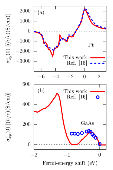
Figure 2: Static SHC of (a) bulk Pt and (b) bulk GaAs calculated in this work as a function of the shift in the Fermi energy relative to its self-consistent value. The results of Refs. Guo et al., 2008, 2005 are also shown for comparison.

IV.2 Static spin Hall conductivities of Pt and GaAs

The static SHC of Pt and GaAs is plotted in Fig. 2 as a function of the shift in Fermi energy relative to its self-consistent value. Physically, this shift can be ascribed to a change in electron density from either alloying (Pt) or doping (GaAs), provided that the electronic structure does not change appreciably in the process (the so-called “rigid-band approximation”).

The results for Pt in Fig. 2(a) are in good agreement with those reported in a previous first-principles study.Guo et al. (2008) The large peaks around the unshifted Fermi level, and $4$ eV below it, are caused by avoided band crossings induced by the spin-orbit interaction.Guo et al. (2008) For p-doped GaAs, Fig. 2(b) shows that the SHC calculated with our method has a peak when the Fermi level is placed $0.3$ eV below the top of the valence bands ($\Delta E_{\rm F}=-0.3~{}$eV), and that it becomes nearly zero when $\Delta E_{\rm F}=-0.8$ eV. This is in contrast to a previous first-princples study,Guo et al. (2005) where it was reported that the intrinsic SHC remains constant at around $120\,(\hbar/e)$ S/cm for $\Delta E_{\rm F}$ between $-0.3$ eV and $-0.8$ eV, as also shown in the figure.

Let us now check the validity for Pt and GaAs of the approximation schemes described in Sec. II.4, starting with projected-spin approximation. As discussed in Sec. II.4.1, in the case of nonmagnetic systems that approximation is valid provided that the Bloch subspace spanned by the MLWFs is left invariant under the action of the spin operator $s^{z}=(\hbar/2)\sigma^{z}$. In the following, we quantity the extent to which this condition is satisfied for each interpolated eigenstate separetely.

We begin by resolving the identity operator as

$$\mathbbm{1}=\sum_{m}{|u^{(\mathrm{H})}_{m\mathbf{k}}\rangle\langle u^{(\mathrm{H})}_{m\mathbf{k}}|}+\sum_{r}{|v_{r\mathbf{k}}\rangle\langle v_{r\mathbf{k}}|}\,,$$ (51)

where the states $\{|v_{r\mathbf{k}}\rangle\}$ span the space of lattice-periodic functions orthogonal to every $|u^{(\mathrm{H})}_{m\mathbf{k}}\rangle$ ($m=1,\ldots,N_{\rm W}$). Inserting Eq. (51) in the identity $1=\left<u^{({\rm H})}_{n{\bf k}}\right|(\sigma^{z})^{2}\left|u^{({\rm H})}_{n{\bf k}}\right>$ we obtain $1=I_{n\bf k}+R_{n\bf k}$, where

$$R_{n\bf k}=\sum_{r}\left|\left\langle v_{r{\bf k}}\middle|\sigma^{z}\middle|u^{({\rm H})}_{n{\bf k}}\right\rangle\right|^{2}$$ (52)

and

$$I_{n{\bf k}} \equiv \sum_{m}\left|\left<u^{({\rm H})}_{m{\bf k}}\right|\sigma^{z}\left|u^{({\rm H})}_{n{\bf k}}\right>\right|^{2}$$ (53)

$$= \sum_{m}\left|\left<u^{({\rm W})}_{m{\bf k}}\right|\sigma^{z}\left|u^{({\rm H})}_{n{\bf k}}\right>\right|^{2}$$

are the weights of the normalized state $\sigma^{z}\left|u^{({\rm H})}_{n\bf k}\right>$ inside and outside the projected Wannier subspace, respectively. Since those weights add up to one, any significant deviation of $I_{n{\bf k}}$ from unity would indicate a failure in the projected-spin approximation.

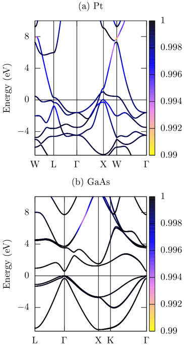
Figure 3: The interpolated band structures of (a) Pt and (b) GaAs, color-coded by the quantity $I_{n{\bf k}}$ given by Eq. (53).

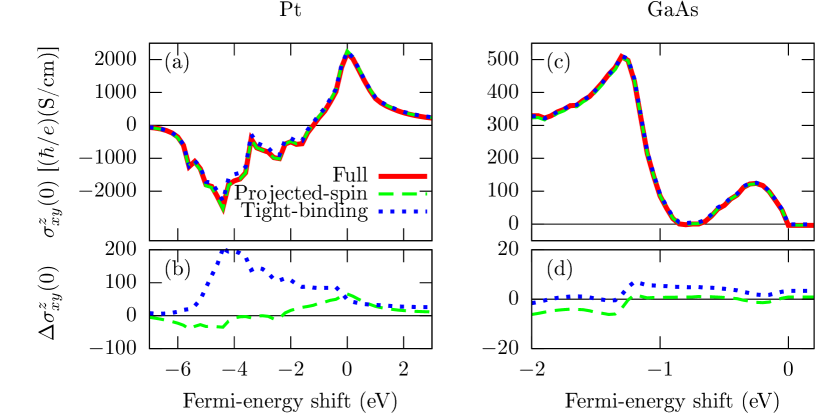
Figure 4: (a) The calculated static SHC of bulk Pt as a function of the shift in the Fermi energy relative to its self-consistent value. The solid red curve is the same as that in Fig. 2(a), and it corresponds to a full Wannier-based calculation of the velocity and spin-current matrix elements, without any approximations. The dashed green curve corresponds to a calculation using the projected-spin approximation of Sec. II.4.1, and the dotted blue curve corresponds to a calculation using the tight-binding approximation of Sec. II.4.2. (b) The difference in the SHC values between each of the two approximate calculations and the full one. (c) and (d) show the same quantities as (a) and (b), but for GaAs.

Figure 3 shows the interpolated energy bands of Pt and GaAs color-coded by the quantity $I_{n{\bf k}}$; this quantity remains very close to unity for every band that is well described by the MLWFs, suggesting that the projected-spin approximation is valid for both materials. This is confirmed by Fig. 4, where it can be seen that the error that it introduces in the calculated SHC is of a few percent at most. (As discussed earlier, that error can be systematically reduced by increasing the number $N_{\rm W}$ of MLWFs per cell.)

Figure 4 also shows the impact on the calculated SHC of the tight-binding approximation of Sec. II.4.2. The error it introduces is again relatively small, of the order of 10%. The reliability of the tight-binding approximation in the context of the Wannier-interpolation scheme suggests that the empirical tight-binding method, with parameters obtained by fitting to either experimental results or first-principles calculations, should yield reasonably good results for the SHC in these classes of materials.

IV.3 Dynamic spin Hall conductivity of GaAs

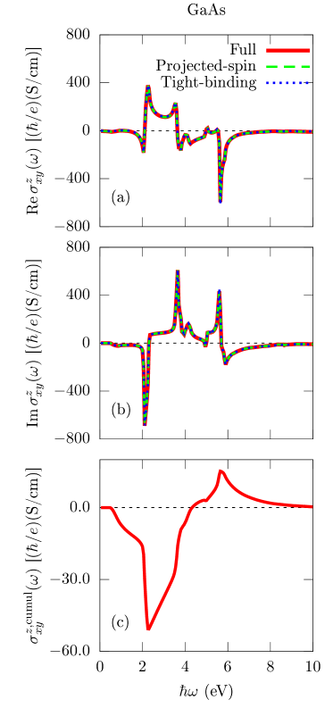
Figure 5: The (a) real and (b) imaginary parts of the dynamic SHC of bulk undoped GaAs. (c) A cumulative integral [Eq. (54)] obtained from the imaginary part of the dynamic SHC.

We conclude this section by discussing the calculated dynamic SHC of undoped GaAs, shown in Figs. 5(a,b). As in the case of the static SHC, the results obtained with the projected-spin and tight-binding approximations are very close to the results of a full calculation. To check the convergence of the static SHC with respect to $N_{\rm W}$ (or equivalently, to the energy range spanned by the MLWFs), we calculate the following function from the imaginary part of the dynamic SHC:

$$\sigma^{z,\mathrm{cumul}}_{xy}(\omega)=\frac{2}{\pi}\int_{0}^{\omega}{d\omega^{\prime}\frac{\mathrm{Im}\,{\sigma_{xy}^{z}(\omega^{\prime})}}{\omega^{\prime}}}\,.$$ (54)

Thanks to the Kramers-Kronig relation, this function converges to the static SHC value (which is zero for undoped GaAs) as $\omega\rightarrow\infty$. As show in Fig. 5(c), $\sigma_{xy}^{z,\mathrm{cumul}}(\omega)$ is already reasonably close to zero by the time $\omega$ reaches 8 eV. This implies that, for the purpose of evaluating the static SHC, one should choose a set of MLWFs that describes accurately the conduction bands of GaAs up to at least 8 eV from the valence-band maximum.

In closing, we note that the dynamic SHC of GaAs reported in Ref. Guo et al., 2005 is blue-shifted by around 1 eV compared to our results in Figs. 5(a,b). Apart from that, the spectra obtained in both works are quite similar in terms of the overall shape, including the positions of the peaks. The reason for the blue shift is that the authors of Ref. Guo et al., 2005 applied the so-called scissor shift in order to correct for the underestimation of the band gap in density-functional theory calculations. We chose not to perform the scissors operation, in order to demonstrate in a transparent manner the Kramers-Kronig relation between the static SHC and the imaginary part of the dynamic SHC.

V Computational benefits of the approximations to the Wannier-interpolation scheme

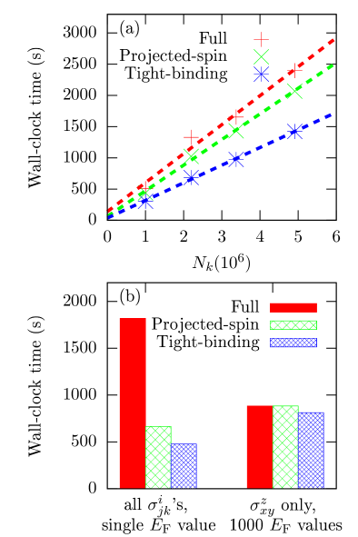
Figure 6: Timings of various benchmark calculations of the static SHC of fcc Pt, comparing the full Wannier-interpolation scheme proposed in this work with the two approximate schemes described in Sec. II.4. (a) The wall-clock time plotted as a function of the number $N_{k}$ of $k$ points on the interpolation grid. The dashed lines are a guide to the eye. (b) The wall-clock time for $N_{k}=10^{6}$, when all 27 components of SHC tensor are calculated independently for the unshifted Fermi level (left), and when only $\sigma^{z}_{xy}$ is calculated for 1000 different values of the Fermi level (right).

In this section, we analyze the gains in numerical efficiency from making the projected-spin and tight-binding approximations when evaluating the SHC. To that end we have measured, for the case of Pt with an unshifted Fermi level, the time elapsed in the subroutine that calculates the static SHC $\sigma^{z}_{xy}(0)$. In all the calculations reported below the workload was distributed across 16 CPUs, with parallelization over the $k$ points of the interpolation grid.

A full (approximation-free) Wannier-interpolation calculation of $\sigma^{z}_{xy}(0)$ requires seven $N_{\rm W}\times N_{\rm W}$ matrices at each $k$ point, namely,

$$\langle u_{m\mathbf{k}}^{{\rm(W)}}|H_{\mathbf{k}}|u_{n\mathbf{k}}^{{\rm(W)}}\rangle\,,$$ (55a)

$$\partial_{j} \langle u_{m\mathbf{k}}^{{\rm(W)}}|H_{\mathbf{k}}|u_{n\mathbf{k}}^{{\rm(W)}}\rangle\text{ with $j=x,y$}\,,$$ (55b)

$$\langle u_{m\mathbf{k}}^{{\rm(W)}}|\partial_{y}u_{n\mathbf{k}}^{{\rm(W)}}\rangle\,,$$ (55c)

$$\langle u_{m\mathbf{k}}^{\rm(W)}|s^{z}|u_{n\mathbf{k}}^{{\rm(W)}}\rangle\,,$$ (55d)

$$\langle u_{m\mathbf{k}}^{\rm(W)}|s^{z}|\partial_{x}u_{n\mathbf{k}}^{\rm(W)}\rangle\,,$$ (55e)

$$\langle u_{m\mathbf{k}}^{\rm(W)}|s^{z}H_{\mathbf{k}}|\partial_{x}u_{n\mathbf{k}}^{\rm(W)}\rangle\,.$$ (55f)

These matrices are evaluated by performing Fourier transforms from real space to $k$ space; the total time spent on those Fourier transforms scales linearly with the number $N_{k}$ of $k$ points, and they constitute the most time-consuming step in the entire calculation. On the other hand, a calculation using the projected-spin approximation requires six matrices: those in Eqs. (55a)–(55d), as well as $\langle u_{m\mathbf{k}}^{{\rm(W)}}|\partial_{x}u_{n\mathbf{k}}^{{\rm(W)}}\rangle$. Finally, when making the tight-binding approximation only the four matrices in Eqs. (55a), (55b), and (55d) are needed.

Figure 6(a) shows that in all three cases the wall-clock time indeed scales linearly with $N_{k}$. Compared to a tight-binding calculation, a full calculation takes 1.7 times as long, and a projected-spin calculation takes 1.4 times as long. These results are consistent with the fact that the projected-spin and full calculations require respectively $6/4=1.5$ times and $7/4=1.75$ times more matrix elements than the tight-binding calculation. Note that the speed-up from the projected-spin approximation alone is quite modest, around 15%.

In low-symmetry crystals, the SHC tensor can have up to 27 independent components. To illustrate this scenario, we have calculated explicitly all 27 components for Pt, disregarding the fact that some are related by symmetry (for example, $\sigma^{z}_{xy}=\sigma^{x}_{yz}$). The full calculation took 3.8 times as long as the tight-binding one, and 2.7 times long as the projected-spin one [see Fig. 6(b)]. To understand these numbers, note that the full calculation requires 28 matrices of size $N_{\rm W}\times N_{\rm W}$ at each ${\bf k}$, namely,

$$\langle u_{m\mathbf{k}}^{(\textrm{W})}|H_{\mathbf{k}}|u_{n\mathbf{k}}^{(\textrm{W})}\rangle,\,\partial_{j}\langle u_{m\mathbf{k}}^{(\textrm{W})}|H_{\mathbf{k}}|u_{n\mathbf{k}}^{(\textrm{W})}\rangle,\,\langle u_{m\mathbf{k}}^{(\textrm{W})}|\partial_{j}u_{m\mathbf{k}}^{(\textrm{W})}\rangle,$$

$$\langle u_{m\mathbf{k}}^{(\textrm{W})}|s^{i}|u_{n\mathbf{k}}^{(\textrm{W})}\rangle,\,\langle u_{m\mathbf{k}}^{(\textrm{W})}|s^{i}|\partial_{j}u_{n\mathbf{k}}^{(\textrm{W})}\rangle,\,\langle u_{m\mathbf{k}}^{(\textrm{W})}|s^{i}H_{\mathbf{k}}|\partial_{j}u_{n\mathbf{k}}^{(\textrm{W})}\rangle.$$

In comparison, the projected-spin and tight-binding calculations requires ten and seven matrices, respectively. This yields estimated speed-ups of 28/10 = 2.8 and 28/7 = 4, respectively, which are quite consistent with the actual speed-ups quoted above.

Consider now a scenario where the static SHC $\sigma^{z}_{xy}(0)$ is evaluated for a large number of Fermi levels (as in Sec. IV.2), or where the dynamic SHC $\sigma^{z}_{xy}(\omega)$ is evaluated for a large number of frequencies (as in Sec. IV.3). In both cases, the time spent interpolating the $k$-space matrix elements becomes small compared to the time spent evaluating the Kubo formula starting from those matrix elements. For example, calculating $\sigma^{z}_{xy}(0)$ on a $100\times 100\times 100$ $k$-point mesh for 1000 Fermi levels takes 880 seconds with the full interpolation approach, and 810 seconds with the tight-binding approximation [see Fig. 6 (b)]. This marginal increase by 8% in efficiency is offset by a loss of accuracy of about 10%. Therefore, in these usage scenarios it is best to perform the full calculation, without further approximations to the matrix elements.

From this series of benchmark calculations, we conclude that the speed-up obtained by making the tight-binding approximation in the Wannier-interpolation scheme varies from marginal to up to a factor of four (depending on the number of independent components of the SHC tensor, and on the number of Fermi-energy or frequency values). The main virtue of the tight-binding approach, however, is that the needed parameters can be obtained by fitting to a first-principles calculation or to experiment, and thus it significantly lowers the barrier for computing the SHC with reasonable accuracy (see Sec. IV.2).

VI Summary

In summary, we have presented a method to calculate the intrinsic SHC of a crystal by interpolating the velocity and spin-current matrix elements using MLWFs. The interpolation is carried out as a post-processing step following a conventional first-principles calculation, taking as input from the ab initio run the matrix elements

$$\left<u_{m{\bf q}}\right|H_{\bf q}\left|u_{n{\bf q}}\right>=\varepsilon_{m{\bf q}}\delta_{mn}\,,\left<u_{m{\bf q}}\middle|u_{n,{\bf q}+{\bf b}}\right>\,,\left<u_{m{\bf q}}\right|s^{i}\left|u_{n{\bf q}}\right>\,,$$

$$\left<u_{m{\bf q}}\right|s^{i}\left|u_{n,{\bf q}+{\bf b}}\right>\,,\left<u_{m{\bf q}}\right|s^{i}H_{\bf q}\left|u_{n,{\bf q}+{\bf b}}\right>$$ (57)

between the set of Bloch eigenstates used for generating the MLWFs. The method was validated by applying it to fcc Pt and zincblende GaAs and comparing the results with previous ab initio calculations for these materials.

In addition, we have considered two different types of approximations that have been frequently used in previous Wannier-based calculations of the SHC: the projected-spin approximation, and the tight-binding approximation. We found that the projected-spin approximation is quite good for both Pt and GaAs, and that at worst it slows down the convergence of the calculated SHC with respect to the number of Wannier functions. As for the tight-binding approximation (which includes the projected-spin approximation), it introduces errors of the order of 10%. This suggests that empirical tight-binding models, with parameters fitted to experimental results or to first-principles calculations, can yield reasonably accurate values for the SHC.

Note added: While we were finalizing this study, we became aware of a related preprint, now published as Ref. Qiao et al., 2018. Although the notation in Ref. Qiao et al., 2018 is different from the one used in the present work, our proposed method is broadly consistent with the one reported therein. The viewpoints and analyses of the two studies are however substantially different. One noteworthy difference is the way in which the last two matrix elements in Eq. (57) are evaluated. Here we calculate them exactly, whereas in Ref. Qiao et al., 2018 they are expressed in terms of the first three by making the approximations

$$\left<u_{m{\bf q}}\right|s^{i}\left|u_{n,{\bf q}+{\bf b}}\right>$$

$$\approx\sum_{l}\,\left<u_{m{\bf q}}\right|s^{i}\left|u_{l{\bf q}}\right>\left<u_{l{\bf q}}\right|\left.u_{n,{\bf q}+{\bf b}}\right>$$ (58)

and

$$\left<u_{m{\bf q}}\right|s^{i}H_{\mathbf{q}}\left|u_{n,{\bf q}+{\bf b}}\right>$$

$$\approx\sum_{l}\,\left<u_{m{\bf q}}\right|s^{i}\left|u_{l{\bf q}}\right>\varepsilon_{l{\bf q}}\left<u_{l{\bf q}}\right|\left.u_{n,{\bf q}+{\bf b}}\right>\,,$$ (59)

where the index $l$ runs over the ab initio Bloch eigenstates at the grid point ${\bf q}$ that were included when constructing the MLWFs. This is similar in spirit to (but more accurate than) the projected-spin approximation of Eq. (41).