A Bayesian Solution to the M-Bias Problem

Abstract

It is common practice in using regression type models for inferring causal effects, that inferring the correct causal relationship requires extra covariates are included or “adjusted for”. Without performing this adjustment erroneous causal effects can be inferred. Given this phenomenon it is common practice to include as many covariates as possible, however such advice comes unstuck in the presence of M-bias. M-Bias is a problem in causal inference where the correct estimation of treatment effects requires that certain variables are not adjusted for i.e. are simply neglected from inclusion in the model. This issue caused a storm of controversy in 2009 when Rubin, Pearl and others disagreed about if it could be problematic to include additional variables in models when inferring causal effects. This paper makes two contributions to this issue. Firstly we provide a Bayesian solution to the M-Bias problem. The solution replicates Pearl’s solution, but consistent with Rubin’s advice we condition on all variables. Secondly the fact that we are able to offer a solution to this problem in Bayesian terms shows that it is indeed possible to represent causal relationships within the Bayesian paradigm, albeit in an extended space. We make several remarks on the similarities and differences between causal graphical models which implement the do-calculus and probabilistic graphical models which enable Bayesian statistics. We hope this work will stimulate more research on unifying Pearl’s causal calculus using causal graphical models with traditional Bayesian statistics and probabilistic graphical models.

1 Introduction

In a causal problem we are interested in understanding the outcome $Y$ of applying treatment $T$ to a user with measured attributes $X$. It is well known that if there exist variables that effect both the treatment assignment $T$ and the outcome $Y$ then these unobserved effects can confound estimates of the treatment effect, a phenomenon known as Simpson’s Paradox [11].

The usual way to minimize confounding is to attempt to do “back door adjustment” (which in practice usually means including the covariates in a regression model [9]) for as many observed covariates as are available, this is despite the risk of M-bias which actually increases if back door adjustment is applied unthinkingly to all available variables. An alternative method for achieving back door adjustment is to use propensity score methods [12].

A storm of controversy started in 2009, when Rubin was asked if there were ever cases where covariates should not be included in a model in the journal Statistics and Medicine [14]. Several discussants responded and a number highlighted that in the presence of a specific structure known as the M-structure adjusting for some variables could increase rather than decrease confounding [10] [15] [14].

Rubin ultimately stated the standard Bayesian position that all variables should be conditioned upon, and removing a variable is an ad hockery [13].

The contribution of this paper is to present a Bayesian solution that follows Rubin’s advice of conditioning on all variables and yet obtains the solution advocated by Pearl and others, where average treatment effects unconditional on the covariate can be identified, but personalized treatment effects conditional on the covariates cannot be. In order to allow Bayesian statistics to be applied to causal problems we introduce a two plates framework for probabilistic graphical models, where there is a mapping between the pre and post intervention graphs used by causal graphical models introduced by Pearl and the two plates in the probabilistic graphical model. The two plates framework differentiates itself by having explicit representation of parameters. The parameters can then in some cases carry information from the observation plate to the intervention plate allowing the identification of causal effects.

It is conjectured, but not proven, that the two plates framework allows probabilistic graphical models to be identifiable under the same conditions as causal graphical models [9], but to have benefits in finite sample problems or in non-identifiable cases.

In Section 2 the Pearl solution is presented, in Section 3 we provide the Bayesian solution, in Section 4 we use Markov chain Monte Carlo (MCMC) to demonstrate the method on a case study. We note the posterior reflects that non-identifiability, but also has some surprising structure. Concluding remarks are made in Section 5.

2 The Pearl Causal Graphical Model Solution for M-Bias

Figure 1: The M-bias Mutilated Causal Graphical Model: left original graph from which the data was collected, right the mutilated graph in which we intervene. Shaded variables are observed, clear variables are latent.

A Causal Graphical Model (CGM) for the M-bias problem is shown in Figure 1. Two hidden variables must be drawn independently $U$ and $W$, conditionally on these variables $Z$ is drawn, conditionally on $U$, $T$ is drawn and conditionally on $W$, finally $Y$ is drawn conditionally on $W$ and $T$.

A researcher is observing $T,Z,Y$ from the system given in Figure 1. and regresses $Y$ on $T$ will be able to determine the (average) treatment effect. However if the researcher follows the advice given by some researchers to include all possible covariates and the variable $Z$ is adjusted for, perhaps surprisingly, erroneous treatment effects will be found, see [3] for more discussion.

The do-calculus can be used to transform a probabilistic specification as given in Figure 1 (left) to (if it is indeed possible) the mutilated specification Figure 1 (right) using three substitution rules given in [9].

In this case we only need the first rule that states that $P(Y|{\rm do}(T),Z)$, can be replaced with: $P(y|{\rm do}(T))$, if $Y$ is independent of $Z$ conditional on $T$ in the mutilated graph. The practical meaning of this result is that a researcher can ignore the observations of $Z$ and build a model that infers an average treatment effect of $T$ on $Y$.

A further curiosity about this problem is that if we observed many realizations of the mutilated graph Figure 1 (right) it would be indeed possible to use $Z$ to produce personalized treatment effects (as $Z$ gives information about $W$ which affects $Y$). However this relationship involving $Z$ cannot be identified from the un-mutilated model Figure 1 (left).

Table 1: Example data set.

T	Z	Y	N
0	0	0	33
0	0	1	2
0	1	0	95
0	1	1	50
1	0	0	100
1	0	1	47
1	1	0	60
1	1	1	240

For purposes of illustration, we assume that $Y,Z,W,T\in\{0,1\}$ and the data is given in Table 1. According to the do calculus we ignore $Z$ and should compute estimates of the average treatment effect which is given by:

$$P(Y=1|T=1)-P(Y=1|T=0)=\frac{47+240}{47+240+100+60}-\frac{50+2}{50+2+33+95}\approx 0.35$$

The source of controversy in this example is that it is not appropriate to apply back door adjustment here. If we were to apply back door adjustment we obtain:

$$P(Y=1|T=1,Z=0)-P(Y=1|T=0,Z=0)=\frac{47}{47+100}-\frac{2}{2+33}\approx 0.26,$$

$$P(Y=1|T=1,Z=1)-P(Y=1|T=0,Z=1)=\frac{240}{240+60}-\frac{50}{50+95}\approx 0.46.$$

This calculation while not causal is valid if you would like to update your belief about records in the observational data where the $Y$ label is missing. Crucially it does not apply to the mutilated graph.

3 The Bayesian Probabilistic Graphical Model Solution for M-Bias

Figure 2: The M-bias Probabilistic Graphical Model. The observational data is in the m=1..M plate where the intervention is given in M+1..N. Parameters explicitly show how information transfers between the pre and post intervention world.

We now repeat the same analysis using Bayesian statistics and probabilistic graphical models (PGM) instead of the do-calculus and causal graphical models (CGM). The appropriate graphical model is given in Figure 2. Some notable differences with the CGM structure are that there are now two plates; one for the original graph (observations $1..M$) and one for the mutilated graph (observations $N+1..M$). As we are now using Bayesian statistics every repeated observation has its own index. Another key difference is that arrow directions in the PGM simply represent a factorization and not causality and can be reversed. The inferential step uses standard Bayesian techniques such as conditionalizing and marginalizing rather than the do-calculus.

The inference problem is to determine $Y_{1..N}$ for some hypothetical $T_{N+1..M}$ and the data $Z_{N+1..M},T_{1..M},Y_{1..M}$.

The full probability specification is

$$P( Y_{1..N},W_{1..N},Z_{1..N},U_{1..N},T_{1..M},\lambda,\phi,\theta,\varphi,\nu|T_{M+1,..N})=$$

$$\left(\prod_{m=1}^{M}P(Y_{m}|W_{m},T_{m},\theta)P(T_{M}|U_{m},\varphi)P(Z_{m}|U_{m},W_{m},\nu)P(U_{m}|\lambda)P(W_{m}|\phi)\right)$$

$$\times\left(\prod_{n=M+1}^{N}P(Y_{n}|W_{n},T_{n},\theta)P(Z_{n}|U_{n},W_{n},\nu)P(U_{n}|\lambda)P(W_{n}|\phi)\right)$$

$$\times P(\lambda)p(\phi)P(\theta)P(\varphi)P(\nu).$$

We note that there is no marginal distribution of $T_{M+1,..N}$ where in contrast $T_{1..M}$ does indeed have a distribution and is dependent on both $Z_{1..M}$ and hidden variables $U_{1..M}$ and $W_{1..M}$, which is precisely why it is hard to identify when the outcome is caused by the treatment and when the allocation of treatments is associated with hidden variables that can predict the outcome.

Once we have the model specified in these terms we are able to predict $Y_{M+1..N}$ conditional on the data and any counter factual $T_{M+1..N}$. This simply takes the form:

$$P(Y_{M+1..N}|W_{1..N},Z_{1..N},U_{1..N},T_{1..M},Y_{1..N},\lambda,\phi,\theta,\varphi,T_{M+1,..N})$$

$$=\frac{\iiint P(Y_{1..N},W_{1..N},Z_{1..N},U_{1..N},T_{1..M},\lambda,\phi,\theta,\varphi|T_{M+1,..N})dW_{1..N}dU_{1..N}d\lambda d\phi d\theta d\varphi}{\iiint P(Y_{1..N},W_{1..N},Z_{1..N},U_{1..N},T_{1..M},\lambda,\phi,\theta,\varphi|T_{M+1,..N})dW_{1..N}dU_{1..N}d\lambda d\phi d\theta d\varphi dY_{M+1..N}}.$$

This is the most direct Bayesian solution to the M-bias problem as posed by Pearl, but it turns out to be difficult computationally. While Bayesian statistics often face high dimensional integrals similar to the above there are two issues that make this problem relatively difficult. The first of these issues is that the role of latent variables in Pearl’s causal graphical model framework and the probabilistic graphical model framework popularized by Jordan [7] and others is quite different. Pearl uses latent variables to represent any and all external complexities that the world may impose on the system, therefore the latent variables may have very large cardinality, in contrast, probabilistic graphical models a latent variable (i.e. an unobserved variable within a plate) is usually present to coerce the model into complete data exponential family form. This enables families of approximating algorithms such as Gibbs sampling [5] and mean field variational Bayes [6].

The second issue is that this model has some parameters that are identifiable and others that are not. Indeed the point of this exercise is that it is possible to infer treatment effects averaging over $Z$, but it is not possible to infer personalized treatment effects adjusting for $Z$. This lack of identifiability means many methods for locally approximating the posterior fail to represent the identifiable and unidentifiable aspects of the posterior - which in this case we are interested in.

We handle these two issues by (a) re-parameterizing the model and analytically marginalizing out $U_{m}$ (which allows $U_{m}$ to have unbounded cardinality), (b) keeping the cardinality of $W_{m}$ to 2 for demonstration purposes and (c) using the MCMC algorithm known as the “the independence sampler”, which while inefficient guarantees exploration of the whole posterior.

Before proceeding it is worth mentioning another key difference between causal graphical models and probabilistic graphical models. In a causal graphical model the direction of an arrow describes the direction of causality, in contrast, a probabilistic graphical model the arrow direction is just highlight one possible factorization which can also be reversed i.e. using the identity $P(a,b)=P(a|b)p(b)=P(b|a)P(a)$ and as such in the probabilistic graphical model framework arrow reversals are permitted

We see straight away that $P(Y|W,Z,\theta)$ is already in a convenient form in both plates. However we have some work to do in simplifying $P(W_{m},U_{m},Z_{m},T_{m}|\varphi,\lambda,\phi,\nu)$ and $P(W_{n},U_{n},Z_{n}|T_{n},\lambda,\phi,\nu)$ in particular factorizing $P(W_{m},U_{m},Z_{m},T_{m}|\varphi,\lambda,\phi,\nu)$ and marginalizing $U_{m}$ (it turns out $W_{m}$ cannot be marginalized without causing the two plates to have different structure:

$$P (W_{m},|Z_{m},T_{m},\varphi,\lambda,\phi,\nu)$$

$$=\frac{\int P(W_{m},U_{m},Z_{m},T_{m}|\varphi,\lambda,\phi,\nu)dU_{m}}{\iint P(W_{m},U_{m},Z_{m},T_{m}|\varphi,\lambda,\phi,\nu)dU_{m}dW_{m}}=P(W_{m}|Z_{m},T_{m},\alpha).$$

where $P(W_{m}|Z_{m},T_{m},\alpha)$ is a re-parameterization integrating over the (possibly) high cardinality $U_{m}$ and $\alpha$ is a transform of the parameters $\varphi,\lambda,\phi,\nu$. In the intervention plate a different computation occurs as knowledge of $T_{n}$ no longer gives any information about $W_{n}$ (this occurs because we set $T_{n}$ ourselves).

$$P (W_{n},|Z_{n},\lambda,\phi,\nu)=\frac{\int P(W_{n},U_{n},Z_{n}|\lambda,\phi,\nu)dU_{m}}{\iint P(W_{n},U_{n},Z_{n}|\lambda,\phi,\nu)dU_{m}dW_{m}}=P(W_{m}|Z_{m},\omega)$$

where $P(W_{m}|Z_{m},\omega)$ is a re-parameterization integrating over the (possibly) high cardinality $U_{m}$ and $\omega$ is a transform of the parameters $\lambda,\phi,\nu$.

We can also do a similar re-parameterization for $P(T_{m}|\kappa)$ and $P(Z|\nu)$ although these quantities are ancillary to the analysis.

Details for the transforms for $\alpha$, $\omega$ in terms of the original parameters are given in the supplementary material.

As $\alpha$ and $\omega$ are both functions of $\lambda,\phi,\nu$ the prior distribution has a dependency i.e. $P(\alpha,\omega)=P(\omega|\alpha)P(\alpha)$, further note that $\alpha$ encodes a distribution that conditions on $T$ where $\omega$ does not as such $\alpha$ is typically of higher dimension than $\omega$. The new parameterization the graph is given in Figure 3.

We briefly comment on the reversal of the arrow direction from the treatment which has the interpretation of $T_{m}$ causes you to think that $W_{m}$ may have certain values, but which is not permitted in a causal graphical model as $W_{m}$ causes $T_{m}$ and the arrow cannot be reversed as the arrow has a causal interpretation. The model can now be written:

Figure 3: The M-bias Graph Probabilistic Graphical Model with arrow Reversals (and $U$ marginalized

$$P (Y_{1..N},W_{1..N},Z_{1..N},\theta,\alpha,\omega,\nu|T_{1..N})=$$

$$\left(\prod_{m=1}^{M}P(Y_{m}|W_{m},Z_{m},\theta)P(W_{m}|Z_{m},T_{m},\alpha)P(Z_{m}|\nu)\right)$$

$$\times\left(\prod_{n=N+1}^{N}P(Y_{n}|W_{n},Z_{n},\theta)P(W_{n}|Z_{n},\omega)P(Z_{n}|\nu)\right)P(\theta)P(\alpha)P(\nu)P(\omega|\alpha)$$

The M-structure prevents the identification of individual treatment effects, yet average treatment effects can be inferred. The identification of $\theta$ is hampered by it involving the latent $W_{m}$, similarly the identification of $\alpha$ is also hampered by the unobserved latent variable, but there is the further problem that $\alpha$ is present in the observation plate, but $\omega$ is in the intervention plate and only $P(\omega|\alpha)$ can transfer information between the plates, and we may contemplate the situation where $P(\omega|\alpha)P(\alpha)=P(\omega)P(\alpha)$ where information simply doesn’t flow.

It is remarkable that in the face of all this poor identifiability that we can recover the M-Bias result found by Pearl. That is we can infer the average treatment effects if not personalized treatments adjusting for $Z$.

We now specify parametric forms for the various terms in the model:

$P(Y_{m}=1|T_{m},W_{m},\theta)=\theta_{T_{m},W_{m}}$	$P(W_{m}|Z_{m},T_{m},\alpha)=\alpha_{W_{m},Z_{m},T_{m}}$
$P(W_{n}|Z_{n},\omega)=\omega_{W_{n},Z_{n}}$	$P(Z_{m}|\nu)=\nu_{Z_{m}}$
$\forall z\hskip 11.38109pt\omega_{:,z}\sim{\rm Dirichlet}(1_{K})$	$\forall z,t\hskip 11.38109pt\alpha_{:,z,t}\sim{\rm Dirichlet}(1_{K})$
$\forall w,z\hskip 11.38109pt\theta_{w,z}\sim{\rm Beta}(1,1)$	$\nu\sim{\rm Dirichlet}(1_{K})$

We also define:

$$\psi_{z,t}=\sum_{w^{\prime}}\theta_{t,w^{\prime}}\alpha_{w^{\prime},z,t}.$$

Which has the interpretation

$$P(Y_{m}=1|Z_{m},T_{m})=\psi_{Z_{m},T_{m}}.$$

The transformed parameter $\psi$ unlike $\theta,\alpha$ is identifiable, but has no causal interpretation (rather it could be used for predicting a missing $Y_{m}$ entry in the first plate only). Using $\psi$ we are able to write the log likelihood function for $\omega,\alpha$ (we can infer $\nu$ separately):

Finally we also define:

$$\rho_{z,t}=\sum_{w^{\prime}}\theta_{t,w^{\prime}}\omega_{w^{\prime},z}.$$

Which has the interpretation

$$P(Y_{n}=1|Z_{n},T_{n})=\rho_{Z_{n},T_{n}}.$$

The transformed parameter $\rho$ is not identifiable, but does have a causal interpretation. We can now write the likelihood:

$$P(Y_{1..M}|X_{1..M},T_{1..M},\psi)=\mathcal{L}(\psi)=\sum_{m}^{M}Y_{m}\log(\psi_{Z_{m},T_{m}})+(1-Y_{m})\log(1-\psi_{Z_{m},T_{m}}).$$

4 Simulation Study on Example using MCMC

A simple inference algorithm is to sample a proposal of the parameters $(\omega^{*},\alpha^{*},\theta^{*})$ from the prior, compute $\psi^{*}$ as a function of the parameters and then evaluate the likelihood to weight the samples i.e. an importance sampling algorithm. A slight variant of the importance sampling algorithm is the MCMC algorithm known as the independence sampler [4]. In this case the proposal distribution is again the prior distribution but a transition is accepted with probability $\mathcal{L}(\psi^{*})+\log P(\omega^{*},\alpha^{*},\theta^{*})-\mathcal{L}(\psi)-\log P(\omega,\alpha,\theta)>\log(u)$, where $u\sim{\rm U}(0,1)$. This algorithm is not efficient, as it does not concentrate exploration on good parts of the posterior however this lack of state is ideal in this case where we have a complex posterior with multiple isolated modes (high posterior regions that are far from each other and therefore difficult to approximate). Markov chain Monte Carlo algorithms such as Gibbs sampling and Hamiltonian Monte Carlo get caught in these isolated modes. This algorithm is ideal for a simple situation such as this but will scale very poorly for more complex problems (or large data sets). Some sophisticated Monte Carlo methods have an improved ability to escape isolated modes e.g. [8] [1].

(a) Personalized Treatment Effect Adjusted for $W$

(b) Personalized Treatment Effect Adjusted for $Z$

(c) Average Treatment Effect

Figure 4: Posterior samples of the treatment effect, adjusted for $W$, adjusted for $Z$ and averaged

We might also be interested in plotting $P(W_{n}|Z_{n})$ but we can note that this is, in this case, completely determined by the prior distribution. As we assume independence i.e. $P(\omega|\alpha)=P(\omega)$, so the posterior of $\omega$ is the same as the prior.

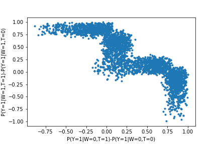
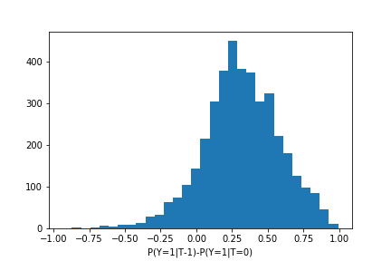
After a burn in of $50000$, we draw $2\times 10^{8}$ MCMC samples but thin them by only retaining every $50000$th sample giving $4000$ samples. In Figure 4 (a) the treatment effect conditional on the unobserved $W$ is shown, where in Figure 4 (b) the treatment effect conditional on the observed $Z$ is shown.

As expected Figure 4 (b) shows that we are unable to determine the personalized treatment effect adjusting for $Z$. The posterior gives support to many possible values and has little structure other than there is some posterior correlation i.e. the treatment effect for $Z=0$ are somewhat more likely to be similar to $Z=1$.

It is also instructive to look at the treatment effects adjusting for the unobservable $W$ in Figure 4 (a), here there is also a lot of uncertainty but there is also some notable structure in that there is an anti-correlation between the treatment effects when $W=0$ and when $W=1$. The “M” shape in the posterior reveals a surprising structure in the posterior, we do not have a complete adequate explanation for this currently and intend to investigate it further.

This anti-correlation is critical to being able to determine the non-personalized treatment effects. This is due to that unconditionally: $P(W=0)=P(W=1)=0.5$ as such the non-personalized treatment effect:

$$P(Y_{m+1}=1|T_{m+1}=1)-P(Y_{m+1}=1|T_{m+1}=0)$$

$$=\left(P(Y_{m+1}=1|T_{m+1}=1,W_{M+1}=0)-P(Y_{m+1}=1|T_{m+1}=0,W_{M+1}=0)\right)P(W_{M+1}=0)$$

$$+\left(P(Y_{m+1}=1|T_{m+1}=1,W_{M+1}=1)-P(Y_{m+1}=1|T_{m+1}=0,W_{M+1}=1)\right)P(W_{M+1}=1),$$

which we can interpret as (half) the sum of the $x$ and $y$ axis in Figure 4 (a), which we can see by eye has much less variance, i.e. when $P(Y=1|W=0,T=1)-P(Y=1|W=0,T=0)$ is high, then $P(Y=1|W=1,T=1)-P(Y=1|W=1,T=0)$ is low and correspondingly the sum of the two is stable. The posterior of the average treatment effect is given in Figure 4 (c).

5 Conclusion

In this paper it was shown that if we follow Rubin’s advice to condition on all variables we recover Pearl’s result that under M-structures average treatment effects are identifiable, yet personalized treatment effects are not. The posterior samples revealed a surprising “M” shape which we do not have an adequate explanation of at this time, but intend to investigate further.

The methodology we use is standard Bayesian statistics using a two plate probabilistic graphical model where one plate represents the observational data and the other the post-intervention data. The two plates could be seen as analogous to the pre and post mutilation graphs in the CGM paradigm.

The two plates framework appears interesting as a general tool for casting causal problems usually analyzed using the do-calculus in a framework that can be analyzed using the vast tools of Bayesian statistics and which includes a methodology that is correct for finite samples and by the use of prior distributions can even draw inference in cases that would be deemed non-identifiable by the do-calculus. It is conjectured that the two plates framework can be proven to recover the identifiability results of the do-calculus.

6 Acknowledgments

The author is grateful for comments on an earlier draft from Noureddine El Karoui, Jeremie Mary, Mike Gartrell and Flavian Vasile which improved the paper. I am especially grateful to Finn Lattimore for many interesting discussions and for every time our intuition disagreed to be another learning opportunity.

References

- [1] M Betancourt. Adiabatic Monte Carlo. arXiv preprint arXiv:1405.3489, 2014.
- [2] B De Finetti. Probabilism. Erkenntnis, 31(2-3):169–223, 1989.
- [3] P Ding and L W Miratrix. To adjust or not to adjust? sensitivity analysis of M-bias and butterfly-bias. Journal of Causal Inference, 3(1):41–57, 2015.
- [4] D Gamerman and H F Lopes. Markov chain Monte Carlo: stochastic simulation for Bayesian inference. Chapman and Hall/CRC, 2006.
- [5] S Geman and D Geman. Stochastic relaxation, Gibbs distributions, and the Bayesian restoration of images. IEEE Transactions on pattern analysis and machine intelligence, pages 721–741, 1984.
- [6] Z Ghahramani and M J Beal. Propagation algorithms for variational bayesian learning. In Advances in neural information processing systems, pages 507–513, 2001.
- [7] M I Jordan. Graphical models. Statistical Science, 19(1):140–155, 2004.
- [8] R M Neal. Annealed importance sampling. Statistics and computing, 11(2):125–139, 2001.
- [9] J Pearl. Causal diagrams for empirical research. Biometrika, 82(4):669–688, 1995.
- [10] J Pearl. Myth, confusion, and science in causal analysis. Statistics in Medicine, 2009.
- [11] J Pearl. Understanding Simpson’s paradox. The American Statistician, 68:8–13, 2014.
- [12] P R Rosenblum and D M Rubin. The central role of the propensity score in observational studies for causal effect. Biometrika, 70(1):41–55, 1983.
- [13] D B Rubin. Should observational studies be designed to allow lack of balance in covariate distributions across treatment groups? Statistics in Medicine, 28(9):1420–1423, 2009.
- [14] I Shrier. Propensity scores. Statistics in Medicine, 28(8):1317–1318, 2009.
- [15] A Sjölander. Propensity scores and M-structures. Statistics in Medicine, 28(9):1416–1420, 2009.