Topological spin excitations in Harper-Heisenberg spin chains

Abstract

Many-body spin systems represent a paradigmatic platform for the realization of emergent states of matter in a strongly interacting regime. Spin models are commonly studied in one-dimensional periodic chains, whose lattice constant is on the order of the interatomic distance. However, in cold atomic setups or functionalized twisted van der Waals heterostructures, long-range modulations of the spin physics can be engineered. Here we show that such superlattice modulations in a many-body spin Hamiltonian can give rise to observable topological boundary modes in the excitation spectrum of the spin chain. In the case of an XY spin-$1/2$ chain, these boundary modes stem from a mathematical correspondence with the chiral edge modes of a two-dimensional quantum Hall state. Our results show that the addition of many-body interactions does not close some of the topological gaps in the excitation spectrum, and the topological boundary modes visibly persist in the isotropic Heisenberg limit. These observations carry through when the spin moment is increased and a large-spin limit of the phenomenon is established. Our results show that such spin superlattices provide a promising route to observe many-body topological boundary effects in cold atomic setups and functionalized twisted van der Waals materials.

I Introduction

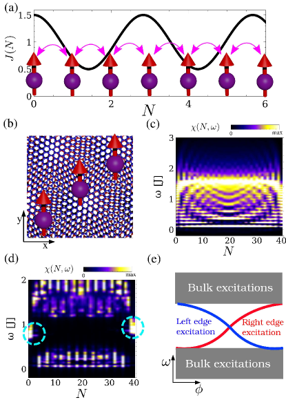
Figure 1: (a) Sketch of a spin chain superlattice with Heisenberg couplings (magenta arrows) modulated in space [cf. Eq. (1)] that can be engineered in a cold atom setup. Moreover, the model of panel (a) naturally arises in atomically engineered lattices on top of twisted van der Waals materials as shown in panel (b). (c) The calculated dynamical structure factor [cf. Eq. (2)] for a uniform $S=1/2$ chain, showing the emergence of different confined modes and a gapless excitation spectrum. (d) The calculated dynamical structure factor of a modulated chain with $\alpha=\pi/\sqrt{2}$, $\lambda=0.5$ and $\phi=0.6\pi$, showing the emergence of a spectral gap and in-gap edge excitations (cyan circles). As the pumping parameter $\phi$ is varied, we expect topological in-gap modes to traverse the bulk gap as sketched in panel (e).

Topological phases of matter comprise one of the most active research domains in contemporary physics research Qi and Zhang (2011); Hasan and Kane (2010). Prominent examples thereof involve systems with translational symmetry, where characteristic topological boundary effects appearQi and Zhang (2011); Hasan and Kane (2010), requiring in certain scenarios an additional symmetry constraint, such as chiralSu et al. (1979), time reversalAvron et al. (1988); Kane and Mele (2005); Qi et al. (2008), or crystallineFu (2011); Chiu et al. (2016) symmetries. Identification of this fundamental source for topology has enabled the realization of topological effects in a plethora of systems including electronic Qi and Zhang (2011); Hasan and Kane (2010), photonic Ozawa et al. (2019), atomic Cooper et al. (2019), phononicLu et al. (2009); Serra-Garcia et al. (2018); Brendel et al. (2018); Süsstrunk and Huber (2015) and circuit metamaterials.Albert et al. (2015); Ningyuan et al. (2015); Imhof et al. (2018); Koch et al. (2010) Additionally, topological phenomena may arise from single-particle interference in structures where competition between different length scales occurs, i.e., in structures with broken lattice translation-invariance. Examples of this include breaking of translation-invariance with magnetic-fields in integer quantum Hall effects Thouless et al. (1982), topological pumps Thouless (1983); Kraus et al. (2012); Lohse et al. (2016, 2018); Zilberberg et al. (2018); Lang et al. (2012), and topological quasicrystals Kraus et al. (2012); Kraus and Zilberberg (2012); Kraus et al. (2013); Verbin et al. (2015); Kraus and Zilberberg (2016). These systems share a deep connection with one another: an adiabatic time-dependent modulation between superlattice potentials sharing the same long-range order can lead to topological pumping and a dynamical realization of quantum Hall systems Thouless (1983); Kraus et al. (2012).

The fundamental motivation for exploring the topology of spectral gaps in physical systems is threefold: (i) nontrivial topology implies topological phase transitions between systems of different topology, (ii) quantized bulk responses appear in association with the topology, and (iii) at open boundaries, the quantized topological bulk invariants lead to corresponding boundary effects Qi and Zhang (2011); Hasan and Kane (2010); Ozawa et al. (2019). For example, the energy levels of the quantum Hall effect are associated with topological invariants – Chern numbers – that lead to the quantization of the bulk Hall conductance. In turn, with open boundary conditions, the quantum Hall effect exhibits corresponding chiral edge modes Qi and Zhang (2011); Hasan and Kane (2010); Ozawa et al. (2019). In similitude, topological pumps exhibit a quantized number of charges pumped per pump-cycle corresponding to the Chern number of the pump  Thouless (1983); Kraus et al. (2012). At their boundaries, 0D boundary modes must appear and cross the spectral gap during the per pump-cycle. Kraus et al. (2012)

Moving towards the design of topological phenomena in many-body quantum systems,Senthil (2015) we consider a variety of platforms including cold atom in optical superlatticesAidelsburger et al. (2014); Boada et al. (2015); Mancini et al. (2015); Stuhl et al. (2015); Li et al. (2016); Goldman et al. (2016); Viebahn et al. (2019), and atomically engineered lattices with scanning tunnel microscopy Choi et al. (2019). These systems allow for the engineering of tailored quantum spin models Loth et al. (2012); Otte et al. (2008); Choi et al. (2017); von Bergmann et al. (2015); Toskovic et al. (2016); Spinelli et al. (2014); Bryant et al. (2015); Yang et al. (2017); Choi et al. (2017); Baumann et al. (2015); Natterer et al. (2017). A particularly versatile candidate in this direction consists of hydrogenated grapheneYazyev (2010), where each hydrogen atom binds an $S=1/2$ state in grapheneGonzalez-Herrero et al. (2016). A key feature of this system, relevant to our work, is that the system can be placed on top of another graphene layer to form a moiré pattern that in turn leads to a long-ranged modulation of the spin-chain’s exchange-couplingsBrihuega and Yndurain (2017); Ramires and Lado (2019). In particular, one can consider a single graphene layer where hydrogen atoms are deposited equidistantly from each other. By placing such a functionalized graphene layer on top of another pristine graphene sheet and at a relative angle, a moire pattern will appear that effectively modulates the spin chain’s exchange constants. These platforms offer the opportunity to study novel phenomena such as many-body quantum phase transitionsCrowley et al. (2018); Vidal et al. (1999); Hida (2001); Vidal et al. (2001); Vieira (2005a); Arlego (2002); Vieira (2005b); Arlego et al. (2001); Roux et al. (2013, 2008); Kraus et al. (2014); Vieira and Hoyos (2018); Friedman and Berkovits (2015) and many-body localizationSetiawan et al. (2017); Mastropietro (2015); Iyer et al. (2013).

In this work, we show that topological boundary modes emerge in the dynamical response spectrum of many-body spin chains with a superlattice modulation. In particular, we focus on isotropic spin chains with modulated exchange constants, that can be realized both in cold-atom setups and the solid-state platform discussed above. We harness a combination of a kernel polynomial method Weiße et al. (2006) with tensor network techniques ite to compute the dynamical structure factors of the many-body system, that exhibit the appearance of topological boundary excitations. We furthermore provide an analytic adiabatic connection to known regimes, showing that in certain paradigmatic cases, the topological modes can be adiabatically connected to a well-understood non-interacting limit. Last, by a systematic scaling-up of the spins’ moment, we obtain that our results persist also in the large-spin limit, showing the universality of such excitations in superlattices.

The manuscript is organized as follows: in Section II.1, we present the topological bulk and boundary effects corresponding to the mapping between free particles in one-dimensional superlattices, topological pumps, and two-dimensional quantum Hall states. This section shows the connection between single particle topological modes and many-body topological response functions. The next sections deal exclusively with topological many-body response functions, in systems that cannot be mapped to a single particle picture. In Sec. III, we detail the kernel polynomial method Weiße et al. (2006) and its utility in showing the emergence of topological boundary excitations in many-body $S=1/2,1,3/2,2$ superlattice chains. We, thus, reveal the existence of topological gaps in the excitation spectrum of many-body superlattices. Finally, in Sec. IV, we discuss and summarize our results.

II Topological pumps and their boundary modes

The main goal of this work is to show that 1D many-body superlattices support topological gaps with in-gap boundary modes in their excitation spectrum. These topological modes arise from the competition between different length scales in the system. In conventional fermionic systems, such modes are associated to a quantized topological pumping response in the bulk. In particular, in the non-interacting limit, these boundary modes support the quantized charge pumping in a finite system Thouless (1983); Kraus et al. (2012). Furthermore, they correspond to the sampling over the chiral edge modes of a parent 2D quantum Hall-like system Kraus et al. (2012). Here, we aim to extend such a mapping to strongly interacting systems, by expressing the existence of topological boundary modes in a many-body framework.

We consider a Heisenberg model with a long-ranged modulation of its exchange constants,Hu et al. (2014, 2015) see Fig. 1(a). Here we focus on spin models whose exchange constants are of the form

$$H=J\sum_{N}[1+\lambda\cos(\alpha N+\phi)]\vec{S}_{N}\cdot\vec{S}_{N+1}\,,$$ (1)

where $\vec{S}_{i}$ are spin operators with spatially-modulated coupling of amplitude $\lambda$, modulation frequency $\alpha$, and displacement $\phi$. The site index $N$ goes from $N=0$ (the leftmost site) to $N=L-1$ (the rightmost site). We note that the impact of non-periodicity on the ground state of quantum Heisenberg models has been addressed in the past.Wessel et al. (2003) As stated previously, the Hamiltonian Eq. (1) can be realized in cold atomic setups and solid-state platforms based on atomically engineered twisted 2D materials [Fig. 1(b)].Wessel et al. (2003); Hida (2004); Ramires and Lado (2019); Brihuega and Yndurain (2017); Lopez-Bezanilla and Lado (2019) In the solid state realization of this Hamiltonian based on hydrogenated twisted bilayer graphene, the parameter $\alpha$ in will be controlled by the ratio between the hydrogen-hydrogen distance and the moire length, whereas the parameter $\phi$ will be controlled by the displacement between the two layers. When $\lambda=0$, the model describes a uniform antiferromagnetic Heisenberg chain. Taking spins $S=1/2$, the spin chain is known to have a gapless excitation spectrum, and represents a paradigmatic integrable system that can be solved using Bethe’s antsaz Faddeev (1996). For arbitrary $\lambda$ and $\alpha$, however, the system has no known solution.

In the following, we will show that a superlattice Hamiltonian of the form Eq. (1) hosts topological boundary modes in its excitation spectrum. The existence of these boundary modes can be seen in the dynamical structure factor

$$\chi(N,\omega)=\langle GS|S_{N}^{z}\delta(\omega-H+E_{0})S_{N}^{z}|GS\rangle\,,$$ (2)

where $S^{z}_{N}$ is the spin operator along $z$ at the site number $n$, $E_{0}$ is the many-body ground-state energy, and $|GS\rangle$ is the many-body ground state of the system. We note that analogous dynamical structure factors can be defined by taking operators for the different spin components, so that the previous one correponds to the $zz$ dynamical structure factor $\chi\equiv\chi^{zz}$. This quantity is sensitive to the spectrum of excitations in the system that are accessible by a local perturbation at position $N$. The details of the method to compute Eq. 2 are detailed in Sec. III.1. Using the dynamical structure factor, we can for example readily verify the aforementioned gapless excitation spectrum property of Eq. (1) for the $S=1/2$ uniform antiferromagnetic Heisenberg chain, see Fig. 1(c). Taking $\lambda\neq 0$, gaps appear in the dynamical structure factor spectrum and topological boundary modes can be observed in the excitation spectrum of the boundary, see Fig. 1(d). In particular, the in-gap modes wind through the bulk excitation gap as a function of $\phi$, see Fig. 1(e). The origin of such in-gap modes can be understood by starting from a modulated non-interacting limit, as we show in the next section.

II.1 Single-particle topological pumps and their bulk-boundary excitation spectrum

Before focusing on the many-body study of excitations of spin chains [Eq. (1)], we first consider a specific non-interacting limit of Eq. (1). The strongly interacting Hamiltonian Eq. (1) can be modified by breaking its rotational symmetry to obtain a spin chain with anisotropic exchange

$$H(\Delta)=J\sum_{N}[1+\lambda\cos(\alpha N+\phi)][{S}^{x}_{N}{S}^{x}_{N+1}$$

$$+{S}^{y}_{N}{S}^{y}_{N+1}+\Delta{S}^{z}_{N}{S}^{z}_{N+1}]\,.$$ (3)

In the limit $\Delta=0$, Eq. (3) becomes the Harper-XY model Giamarchi (2003) $H(\Delta=0)=\sum_{N}[1+\lambda\cos(\alpha N+\phi)][{S}^{x}_{N}{S}^{x}_{N+1}+{S}^{y}_{N}{S}^{y}_{N+1}]$, which can be analytically solved by means of Jordan-Wigner’s transformation Giamarchi (2003) $S^{-}_{N}=e^{\sum_{i<N}c_{i}^{\dagger}c_{i}}c_{N}$ and $S^{+}_{N}=e^{\sum_{i<n}c_{i}^{\dagger}c_{i}}c^{\dagger}_{N}$, with $S^{\pm}_{N}=S^{x}_{N}\pm iS^{y}_{N}$. Specifically, using the transformation, the Hamiltonian becomes

$$H=t\sum_{N}[1+\lambda\cos(\alpha N+\phi)]c_{N}^{\dagger}c_{N+1}+h.c.\,,$$ (4)

with $t=J/2$. The model Eq. (4) in known as the off-diagonal Harper model,Harper (1955); Kraus and Zilberberg (2012) which was used in the realization of photonic topological pumps.Kraus et al. (2012); Zilberberg et al. (2018) Specifically, it exhibits bulk gaps and topological boundary modes that thread through the gaps as a function of a scan of the pump parameter $\phi$, see Fig. 2(a). The appearance of these in-gap modes stems from the topological quantized bulk response of the pump, which can be traced back to a two-dimensional quantum Hall model on a lattice using dimensional extension. Thouless et al. (1982); Hatsugai (1993); Ozawa et al. (2019); Kraus et al. (2012); Kraus and Zilberberg (2012); Mei et al. (2019)

For completeness, we detail the relationship between the 1D topological pump and the 2D QHE. Let us start with a two-dimensional quantum Hall tight-binding model with nearest-neighbor hopping in the $x$-direction and next-nearest-neighbor hopping along the $\pm x\pm y$-direction [see Fig. 2(b)]

$$H= \sum_{N,M}\Big{[}t\,c_{N,M}^{\dagger}c_{N+1,M}+\frac{\lambda}{2}\Big{(}e^{i\alpha N}c_{N,M}^{\dagger}c_{N+1,M+1}$$

$$\qquad+e^{-i\alpha N}c_{N,M}^{\dagger}c_{N+1,M-1}\Big{)}+h.c.\Big{]}\,.$$ (5)

We have written the model in the Landau gauge and used Peierls’ substitutionPeierls (1933) to describe the magnetic flux piercing each plaquette of the model. In this gauge, the model does not depend on $y$ explicitly and it can be written in terms of momenta $k_{y}$ as good quantum numbers, leading to a summation over Eq. (4) with $k_{y}\equiv\phi$. In other words, superlattice Hamiltonians can be understood to be specific $k$-cuts of a two-dimensional Hall state, where the magnetic flux $\alpha$ competing with the lattice translation in 2D is mapped onto the superlattice modulation frequency in 1D.

For rational values of $\alpha/(2\pi)$, periodic boundary conditions can be found in the $x$-direction with an additional momentum $k$. Correspondingly, a Chern numberXiao et al. (2010) can be computed for occupied bands of the model $\mathcal{C}=\frac{1}{2\pi}\int\Omega_{\alpha k}dkd\phi$, where $\Omega_{\alpha k}=i[\sum_{j\in\mathcal{O}}\partial_{k}\langle\Psi_{j}|\partial_{\phi}\Psi_{j}\rangle-\partial_{\phi}\langle\Psi_{j}|\partial_{k}\Psi_{j}\rangle]$, $\mathcal{O}$ denotes the set of occupied states, and $\Psi_{N}$ are the eigenstates of the system, which for simplicity we assume to be non-degenerate. In the case of a degenerate spectra, the Chern number can be efficiently computed by means of the Wilson loop technique.Soluyanov and Vanderbilt (2011)

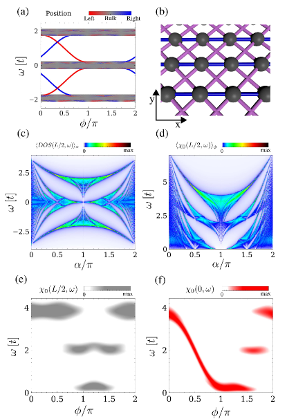
Figure 2: Single-particle superlattices. (a) The energy spectrum of the off-diagonal Harper model [Eq. (4)] as a function of the pumping parameter $\phi$. Topological in-gap bound states appear on both sides of the chain (red and blue), and traverse the gap. The appearance of these states is in correspondence with the topological bulk response of the topological pump and can be mapped to the chiral edge modes of the 2D quantum Hall effect Kraus et al. (2012). (b) Sketch of the 2D quantum Hall model [Eq. (II.1)] that is mappable to the off-diagonal Harper pump [Eq. (4)]. The Hofstadter spectra in a bulk site averaged over $\phi$ (c) and the corresponding dynamical charge response in a bulk site averaged over $\phi$ (d) [cf. Eq. (6)]. Panels (c,d) highlight their characteristic topological spectral gaps for arbitrary $\alpha$. Note the different energy axis in (c) and (d) due to the fact that the dynamical correlator includes contributions from transitions that can have absolute energy $0\leq\omega\leq W$, where $W=\omega_{\rm max}-\omega_{\rm min}$ is the full bandwidth of the bulk spectrum (c). (e) There are bulk gaps that remain open in the dynamical charge response as a function of $\phi$. (f) Same as (e) but evaluated at the boundary, showing in-gap boundary excitations. We used $\lambda=0.8$ and $\alpha=\pi/\sqrt{2}$ in (acdef), panels (c) and (d) are averaged over $\phi$.

The existence of a non-zero Chern number for the pump [Eq. (4)] implies that for open boundary conditions the system will develop a quantized topological bulk responseThouless (1983); Thouless et al. (1982); Verbin et al. (2015); Schulz-Baldes et al. (1999); KELLENDONK et al. (2002); Klitzing et al. (1980) with associated boundary modes, see Fig. 2(a). In particular, the modes that traverse the gap as a function of $\phi$ appear in pairs that are located at opposite boundaries of the modulated chain, where the number of such pairs equals the Chern number of the gap. In this way, for a specific chain at a particular $\phi$, a certain in-gap state can be located inside the gap, whose origin can be traced back to the non-trivial Chern number of the parent Hamiltonian Kraus et al. (2012). For arbitrary $\alpha$ and $\lambda$, the bulk of the non-interacting superlattice chain [Eq. (4)] will have a fractal hierarchy of gaps with different Chern numbers Thouless et al. (1982); Thouless (1983); Avron et al. (2000). Plotting the bulk density of states as a function of $\alpha$ shows these different gaps forming the so-called Hofstadter butterfly spectrumHofstadter (1976); Chang and Niu (1995), see Fig. 2(c). Since these gaps have non-trivial Chern numbers, the boundary of the system will host in-gap modes.

Such a topological bulk-boundary correspondence analysis cannot be easily extended to many-body systems, due to the fact that direct access to all many-body eigenstates is in general not possible. In order to make the connection with a many-body system, it is useful to demonstrate the non-interacting limit using an response that can be easily defined for a many-body system: a dynamical correlation function.

II.2 Topological pumps in a many-body framework

In a many-body system, the existence of topological boundary modes is defined by means of dynamical quantities instead of by single-particle eigenvalues. As an example, let us consider the non-interacting Hamiltonian Eq. 4: the charge-charge correlation carries information on the single-particle spectrum of the system, and is analogous to the $ZZ$ spin correlator [Eq. (2)] of the original $XY$ model [Eq. (3)]. Therefore understanding the non-interacting limit provides a fruitful starting point to understand the many-body case.

The onsite charge-charge dynamical correlator can be expressed as

$$\chi_{0}(N,\omega)=\langle GS|c^{\dagger}_{N}c_{N}\delta(\omega-H+E_{GS})c^{\dagger}_{N}c_{N}|GS\rangle\,,$$ (6)

where $E_{GS}$ is the many-body ground state energy and $|GS\rangle$ the many-body ground state wavefunction. For free fermions, the previous charge-charge correlator can be computed from the single particle orbitals and eigenvalues of Hamiltonian Eq. 4 by means of Kubo’s formalism as $\chi_{0}(N,\omega)\sim\text{Im}\left(\sum_{\mu,\nu}\frac{f_{\mu,\nu}}{E_{\mu}-E_{\nu}-\omega+i0^{+}}\right)$, with $f_{\mu,\nu}=|\Psi_{\mu}(N)|^{2}|\Psi_{\nu}(N)|^{2}[n(E_{\mu})-n(E_{\nu})]$, $n(x)$ the Fermi-Dirac distribution at $T=0$ (i.e. a step function) and $\Psi_{\mu}$ the single-particle eigenstates corresponding to single-particle eigenenergies $E_{\mu}$. We note that the filling of the free fermion model has to be taken at half filling i.e., with the chemical potential at $\omega=0$, which is the situation mathematically equivalent to the spectral function of the XY model. Calculations away from half filling in the fermionic model are analogous to an XY model with external magnetic field. We emphasize that the many-body response function of Eq. 6 can be thus characterized from the single particle eigenvalues of Eq. 4, making a connection between a many-body response function and single particle energies.

The spectral weight of $\chi_{0}$ can be understood as a weighted convolution of the density of states of the system. The response with the highest energy is expected at $\omega\approx 4t$, since it corresponds to transitions between the deepest occupied state (located at $\omega\approx-2t$) and the highest unoccupied state (located at $\omega\approx+2t$). For a system showing different gaps in its spectra, $\chi_{0}$ will exhibit this structure in a convoluted fashion. We can now compute the bulk $\chi_{0}$ at position $L/2$ where $L$ is the length of the chain and average over different $\phi$. We plot $\langle\chi_{0}(L/2,\omega)\rangle_{\phi}=\frac{1}{2\pi}\int_{0}^{2\pi}\chi_{0}(L/2,\omega,\phi)d\phi$ in Fig. 2(d) for the off-diagonal Harper model Eq. (4). First, we observe that the fractal gap structure in the energy spectra in Fig. 2(c) is indeed manifesting in Fig. 2(d). Importantly, when the bulk gaps remains open, the in-gap excitations located at the boundary of the system generate a signal in the local response. The latter is clearly seen in Figs. 2(e)-(f), where we observe that inside a finite excitation spectral gap of the bulk Fig. 2(e), there are in-gap boundary excitations in Fig. 2(f) that cross the gap as a function of $\phi$. These in-gap excitations stem from the convolution of the original single-particle topological pump modes shown in Fig. 2(a). As a result, the non-trivial boundary phenomenon of the 1D topological pump is observable in the dynamical charge susceptibility.

The previous formulation of pumping modes in terms of a dynamical response has the advantage that it can be also defined for a purely many-body system, where single-particle energies are no longer defined. In the next sections we will explore in system that no longer have single particle excitations, and thus require to compute the dynamical response function from the many-body ground state explicitly. In the following, we will use such formulation to show the emergence of topological edge modes in modulated spin Heisenberg models, a paradigmatic example of a modulated quantum many-body Hamiltonian.

III Boundary excitations of topological pumps in many-body systems

The mapping between a one-dimensional cosine-like long-wavelength modulated Hamiltonian and a two-dimensional quantum Hall state is valid in the free electron case. However, for strongly interacting superlattice Hamiltonians, such a mapping cannot be readily done. In the following, our main goal is to address whether boundary effects corresponding to topological pumps appear also in a many-body dynamical response for generic modulated quantum Heisenberg models.

Excitations in one dimensional $S=1/2$ models are usually studied by means of Jordan-Wigner’s transformation and bosonization techniques Giamarchi (2003). In this framework, low-energy excitations are understood by means of Luttinger liquid excitations Giamarchi (2003). This approximation, however, holds only for small energies, which makes predictions concerning high-energy excitations difficult. To treat high-energy excitations, matrix-product techniques are very well suited, as they allow to exactly solve one-dimensional Hamiltonians without relying on a low-energy approximation. In the following, we harness a combination of a tensor-network formalism together with kernel polynomial techniques to compute dynamical structure factors, and show that superlattice many-body systems can host topological boundary modes in their excitation spectrum. We now elaborate on the numerical procedure that allows us to compute the dynamical properties of the superlattice Heisenberg Hamiltonian Eq. (1).

III.1 Dynamical correlators with the DMRG-KPM method

The kernel polynomial methodWeiße et al. (2006) (KPM) allows for the computation of the function $\chi$ directly in frequency space, by performing expansion in terms of Chebyshev polynomials. For simplicity, we focus our discussion on a Hamiltonian $\bar{H}$ whose ground state energy is located at $E=0$ and whose excited states are restricted to the interval $[0,1)$, which can be generically obtained by shifting and rescaling the original Hamiltonian $H\rightarrow\bar{H}$. The dynamical correlator $\chi$ for the original Hamiltonian $H$ can then be recovered by rescaling back the energies in the dynamical correlator $\bar{\chi}$ of the scaled Hamiltonian $\bar{H}$.

The dynamical correlator $\bar{\chi}$ for the Hamiltonian $\bar{H}$ takes the form

$$\bar{\chi}(\omega)=\langle GS|S_{N}^{z}\delta(\omega-\bar{H})S_{N}^{z}|GS\rangle\,,$$ (7)

where $|GS\rangle$ is the many-body ground state of the system. To compute the dynamical correlator, we perform an expansion of the form

$$\bar{\chi}(\omega)=\frac{1}{\pi\sqrt{1-\omega^{2}}}\left(\mu_{0}+2\sum_{l=1}^{N_{P}}\mu_{l}T_{l}(\omega)\right)\,,$$ (8)

where $T_{l}$ are Chebyshev polynomials. The coefficients of the expansion $\mu_{l}$ can be then computed as

$$\mu_{l}=\int_{-1}^{1}\bar{\chi}(\omega)T_{l}(\omega)d\omega\,,$$ (9)

which can be rewritten as

$$\mu_{l}=\langle GS|S_{N}^{z}T_{l}(\bar{H})S_{N}^{z}|GS\rangle\,.$$ (10)

Taking into account the recursion relation of the Chebyshev polynomials

$$T_{l}(\omega)=2\omega T_{l-1}(\omega)-T_{l-2}(\omega)\,,$$ (11)

with $T_{1}(\omega)=\omega$ and $T_{0}(\omega)=1$, the different coefficients $\mu_{l}$ can be computed by iteratively defining the vectors

$$|{w_{0}}\rangle = S_{N}^{z}|GS\rangle$$ (12)

$$|w_{1}\rangle = \bar{H}|w_{0}\rangle$$ (13)

$$|w_{l+1}\rangle = 2\bar{H}|w_{l}\rangle-|w_{l-1}\rangle\,,$$ (14)

so that $|w_{l}\rangle=T_{l}(\bar{H})S_{N}^{z}|GS\rangle$.

In this way, the coefficients $\mu_{l}$ are computed as

$$\mu_{l}=\langle GS|S_{N}^{z}|w_{l}\rangle\,.$$ (15)

To improve the convergence rate of the expansion, the coefficients are redefined $\mu_{l}\rightarrow g_{l}^{N_{P}}\mu_{l}$, using the Jackson KernelJackson (1912) $g_{l}^{N_{P}}=\frac{(N_{P}-l-1)\cos\frac{\pi l}{N_{P}+1}+\sin\frac{\pi l}{N_{P}+1}\cot\frac{\pi}{N_{P}+1}}{N_{P}+1},$ to damp Gibbs oscillations Weiße et al. (2006). The number of polynomials used $N_{P}$ controls the natural smearing of the $\delta(x)$ function, yielding a smearing that scales as $1/N_{P}$ in units of the whole bandwidth. In particular, the bigger the number of polynomials $N_{P}$, the sharper the spectral features will be. Given that the bandwidth of the full Hamiltonian scales as $S^{2}L$, the smearing in units of the exchange coupling scales as $S^{2}L/N_{P}$. As a reference, we took up to $N_{P}=4000$ for the $S=1/2$ calculations, and $N_{P}=60000$ for $S=2$ calculations. With these coefficients, the dynamical structure factors in the whole frequency range can be computed with the same resolution using Eq. (8). The previous procedure can be used also to compute dynamical correlators between different sites simply by replacing the operator $S_{N}^{z}$ in Eq. (15).

Importantly, the KPM-workflow can be readily implemented within the matrix product state formalismWhite (1992); Schollwöck (2005); Stoudenmire and White (2013) using ITensor ite , that enables usdmr to compute the dynamical correlation function of many-body systems directly in frequency space.Wolf et al. (2014, 2015); Halimeh et al. (2015); Ganahl et al. (2014) In the following, we demonstrate the power of this method in identifying boundary modes of topological pumps in the excitation spectrum of different spin superlattices.

III.2 Boundary excitations of topological pumps in S=1/2 chains

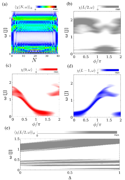
Figure 3: (a) Dynamical structure factor $\chi(\omega)$ [Eq. (2)] in the different sites of the chain averaged over $\phi$ for a Heisenberg spin chain $S=1/2$ of Eq. (1). It is observed that the bulk of the chain shows a spectral gap, whereas at the edge the average spectral function $\langle\chi(\omega)\rangle_{\phi}$ signals the appearance of edge excitations. This can be explicitly seen by looking at the dynamical structure factor $\chi(\omega)$ in the bulk (b), left edge (c) and right edge (d) as a function of $\phi$, showing states that thread through the gap at the edge while the bulk shows a robust spectral gap at the high energy part of the spectrum. The edge modes that pump with $\phi$ can be adiabatically connected to the ones found in the non-interacting limit Fig. 2. Panel (e) shows the bulk dynamical correlator in the anisotropic case $\Delta\neq 1$, showing that the main excitation gap remains open as one goes from the non-interacting ($\Delta=0$) to the fully interacting ($\Delta=1$) limit. We took $\lambda=0.5$ for panels (a,b,c,d,e), $\alpha=0.66\pi$ for (a,e) and $\alpha=0.7\pi$ for (b,c,d).

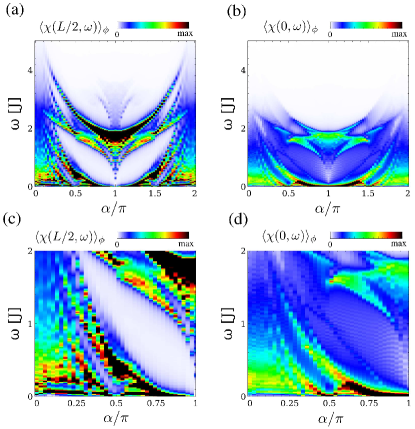
Figure 4: (a-d) Dynamical structure factor $\chi(\omega)$ Eq. (2) averaged over $\phi$, for a Heisenberg spin chain $S=1/2$ of Eq. (1), for different modulation wavevectors $\alpha$. Panel (a) (zoom in (c)) shows the bulk and panel (b) (zoom in (d)) shows the edge $\chi(\omega)$. It is observed that whereas the bulk (a,c) shows a spectral gap, the (b,d) shows a non-zero spectral weight, reflecting the emergence of the edge modes at arbitrary modulation frequencies $\alpha$. In the absence of $ZZ$ interaction in the Heisenberg model Eq. (1), panels (a,c) would be equivalent to panel Fig. 2d. We took $\lambda=0.8$ for panels (a,b,c,d).

We first focus on a spin chain with $S=1/2$, as it represents a minimal many-body system whose topology can be adiabatically connected to a non-interacting limit discussed in Sec. II.1. We consider a spin superlattice chain described by the Hamiltonian 1. Due to the rotational symmetry of Eq. (1), the different correlation functions are equivalent $\chi^{xx}(N,\omega)=\chi^{yy}(N,\omega)=\chi^{zz}(N,\omega)$, which allows us to fully characterize the state by means of a single spin orientation $\chi(N,\omega)\equiv\chi^{zz}(N,\omega)$. Moreover, it is worth to recall the sum rule for the dynamical correlator $\int\chi(\omega)d\omega=\langle GS|(S_{N}^{z})^{2}|GS\rangle$, which for $S=1/2$ yields $\int\chi(\omega)d\omega=1/4$. This sum rule implies that the spectral weight is conserved, and thus sites that yield a finite in-gap response must compensate by decreasing their response in another energy window.

We compute the dynamical structure factor $\chi(N,\omega)$ [Eq. (2)] at each site of the chain, and average over different pump parameters $\phi$, as shown in Fig. 3(a). Whereas the bulk of the system hosts an excitation gap, at the boundaries in-gap excitations appear. A more detailed picture is obtained by comparing the dynamical structure factor in the bulk and at the boundary as a function $\phi$, see Figs. 3(b,c,d), respectively. In the bulk, we observe a gap in the excitation spectrum [Fig. 3(b)], whereas at the boundary excitations cross the gap as a function of $\phi$ [Figs. 3(c) and (d)]. This is the very same phenomenon that we detailed in the non-interacting case [Figs. 2(e) and (f)], showing that topological gaps of excited states of the non-interacting model survive the onset of many-body interactions, and appear in the dynamical response of the system.Mastropietro ; Mastropietro (2016); Apalkov and Chakraborty (2014)

The emergence of topological boundary modes as a function of $\phi$ happens for arbitrary values of $\alpha$. First, let us recall that in the non interacting limit, the value of $\alpha$ was associated to the magnetic field of the parent two-dimensional Hamiltonian, and thus edge modes appear for arbitrary values of $\alpha$. By adiabatically connecting the non-interacting Hamiltonian Eq. (4) to Eq. (1) by means of Eq. (3), we have observed gaps that do not close that support in-gap boundary modes in the fully interacting limit for arbitrary values of $\alpha$. In particular, we show in Fig. 3e the bulk spectral function of Eq. (3) as a function of $\Delta$, observing a bulk gap that remained open for $\Delta\in(0,1)$. In the strongly interacting limit of $\Delta=1$, the existence of such bulk spectral gap and edge modes can be observed by computing the dynamical structure factor as a function of $\alpha$ both in the bulk and at the edge as shown in Fig. 4. In particular, we observe that whereas the bulk shows a robust spectral gap [Figs. 4(a) and (c)], the boundary shows a finite spectral density in that very same energy window [Figs. 4(b) and (d)], highlighting the emergence of in-gap boundary modes for arbitrary modulation frequency $\alpha$.

The adiabatic connection between the Heisenberg model and free fermions is done by means of Eq. (3), which in particular breaks rotational symmetry in the Heisenberg Hamiltonian. Such rotational symmetry breaking makes the different dynamical correlators $\chi^{zz}$ and $\chi^{xx}$ quantitatively different. This motivates us to consider a mapping that retains the spin rotational symmetry between the non-interacting limit and the interacting one. Interestingly, besides the Jordan-Wigner mapping introduced in Sec. II.1 the persistence of the topological boundary modes can be mapped to completely different free model, namely a Harper-Hubbard model. This additional mapping to a free fermionic system does not break the rotational symmetry of the Hamiltonian, in strike comparison with Eq. (3).

To perform the mapping to the Harper-Hubbard model, let us consider a fermionic model similar to Eq. (4), but now for spinful fermions with an onsite Hubbard interaction

$$\centering\begin{split}H_{\phi}=U\sum_{N}c_{N,\uparrow}^{\dagger}c_{N,\uparrow}c_{N,\downarrow}^{\dagger}c_{N,\downarrow}+\\ t\sum_{N}[1+\lambda\cos(\alpha N+\phi)]c_{N,s}^{\dagger}c_{N+1,s}+h.c.\end{split}\@add@centering$$ (16)

For $U=0$, the imaginary part of the spin susceptibility of the previous Hamiltonian can be written as $\chi_{0}(N,\omega,\phi)\sim\sum_{\mu,\nu}\frac{f_{\mu,\nu}}{E_{\mu}-E_{\nu}-\omega+i0^{+}}$, with $f_{\mu,\nu}=\langle\Psi_{\mu}|S^{+}_{N}|\Psi_{\nu}\rangle\langle\Psi_{\nu}|S^{-}_{N}|\Psi_{\mu}\rangle[n(E_{\mu})-n(E_{\nu})]$ and $\Psi_{\mu}$ the different single particle eigenstates of Eq. 16 for $U=0$. Note that the previous expression is equivalent to the charge susceptibility in the absence of symmetry breaking for the spinless chain presented in Sec. II.1. In particular, such susceptibility will have analogous properties as the charge susceptibility of the spinless fermionic chain in the non-interacting limit. As a result, in the limit $U=0$ the spin response can be understood in the same way as the spinless fermionic free case. For increasing values of $U$, the charge fluctuations of the system develop a global gap that scales with $U$, whereas the spin excitations are substantially less affected due to spin-charge separation. In particular, we observe that the high energy gaps in the dynamical spin-spin correlator remain open up to large values of $U$. In particular, for large values of $U$, we can perform a Hubbard-Stratonovic transformation to the Hamiltonian Eq. (16) and map it to the very same Hamiltonian in Eq. (1), with $J=4t^{2}/U$. As a result, the spin excitations in the non-interacting limit adiabatically evolve towards the interacting limit, and thus its topological properties can be once more inferred from the non-interacting scenario.

In this section we have shown that the edge modes of a modulated Heisenberg $S=1/2$ chain can be adiabatically connected to the topological modes of a non interacting limit. This connection can be made both by means of a Jordan-Wigner mapping to an interacting spinless fermion model, or through a Hubbard-Stratonovic transformation to a spinful Hubbard model. Irrespective of the mapping, the analytic connection highlights the topological origin of the edge modes in the modulated $S=1/2$ Heisenberg model. In the following we address the next step in complexity, namely a modulated $S=1$ Heisenberg model, where the previous two mappings are not trivially applied.

III.3 Boundary excitations of topological pumps in S=1 chains

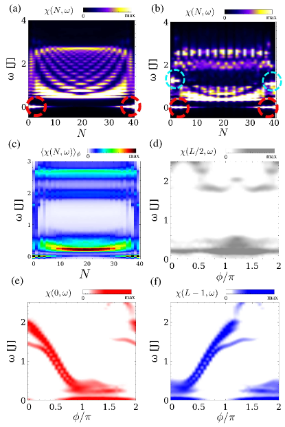
Figure 5: (a) Dynamical structure factor in the different sites of the chain for a uniform $S=1$ Heisenberg model, showing the emergence of topological modes at the edge (red circles). Panel (b) shows the dynamical structure factor for a modulated $S=1$ chain, showing the coexistence of the preexisting zero modes (red circles) with the topological pumping modes (cyan circles). Panel (c) shows the dynamical structure factor for the different sites of a $S=1$ chain averaged over $\phi$. Bulk (d), left edge (e) and right edge (f) dynamical structure factors as a function of $\phi$, showing states that thread through the gap in the edge while the bulk shows an excitation gap in the high energy part of the spectrum. We took $\alpha=\pi/\sqrt{2}$ for panels (b,c,d,e,f), $\lambda=0.4$ for panel (b) and $\lambda=0.7$ in panels (c,d,e,f).

We now address the existence of boundary excitations associated with a topological pump in a Heisenberg chain with $S=1$. In striking comparison with the $S=1/2$ chains studied above, $S=1$ chains are much harder to theoretically study as they cannot be easily connected to a non-interacting limit and, as a result, we directly address the system using a full many-body formulation of topological boundary modes. In the following, we show that despite the missing non-interacting limit, modulated $S=1$ chains show similar topological in-gap excitations.

It is instructive first to address the known limit of $\lambda=0$, that corresponds to a uniform $S=1$ Heisenberg model. This model is known to develop a bulk gap, which has been shown numerically to converge to a value of $0.41J$ in the thermodynamic limit.White (1992) Moreover, such model develops gapless edge modes,White (1992) namely, the Heisenberg model with $S=1$ has the particularity of hosting in-gap boundary modes that originate from its topological non-trivial ground-state. Importantly, these modes appear without the requirement of a superlattice modulation, see Fig. 5(a). As a result, for weak superlattice modulations, the Hamiltonian can host simultaneously boundary modes originating from the original non-trivial topology of the uniform limit [red circles in Fig. 5(b)], and also pumping boundary modes arising from the longer-ranged superlattice modulation [cyan circles in Fig. 5(b)]. For strong modulations, the original topological gap of the uniform system closes and only the topological pumping modes of the superlattice survive.

We now proceed in an analogous way to the free electron limit [Sec. II.1] and to the $S=1/2$ [Sec. III.2]. First, in Fig. 5(c), we show the local dynamical correlator at every site of an $S=1$ chain with open boundary conditions. When averaged out over the different phases $\phi$, the bulk of the $S=1$ spin chain shows an excitation gap as shown in Fig. 5(c), alongside a finite spectral weight on the boundaries in that very same gap. This phenomenon is the same as the one observed for the $S=1/2$ chain [cf. Fig. 3(a)]. The nature of the edge weight can be understood by looking at the $\phi$-dependent dynamical structure factor. In particular, in the bulk, it is observed that a spectral gap appears for every $\phi$, see Fig. 5(d). In comparison, at the boundary [Figs. 5(e) and (f)], we see a pumping in-gap excitation that traverses the gap as $\phi$ is varied.

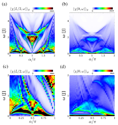
Figure 6: (a-d) Dynamical structure factor $\chi(\omega)$ Eq. (2) averaged over $\phi$, for a Heisenberg spin chain $S=1$ of Eq. (1), for different modulation wavevectors $\alpha$. Panel (a) (zoom in (c)) shows the bulk and panel (b) (zoom in (d)) shows the edge $\chi(\omega)$. It is observed that whereas the bulk (a,c) shows a spectral gap, the boundary (b,d) shows a non-zero spectral weight, reflecting the emergence of the boundary modes at arbitrary modulation frequencies $\alpha$. In contract with the $S=1/2$ chain of Fig. 4, the present case cannot be adiabatically connected to the free fermion Hamiltonian Eq. (4). We took $\lambda=0.8$ for panels (a,b,c,d).

The existence of a high energy bulk excitation gap together with in-gap edge modes emerges for generic modulation frequencies of the Heisenberg superlattice. This can be easily observed by computing the Hofstadter spectra for the modulated $S=1$ chain for different frequencies $\alpha$, see Fig. 6. In particular, we see that a spectral gap appears for a wide range of modulation frequencies $\alpha$ [Figs. 6(a) and (c)]. For any of those frequencies, computing the structure factor at the boundary shows the existence of in-gap modes, see Figs. 6(b) and (d).

For the $S=1$ studied above, no mapping to a free interacting limit can be easily performed. Nevertheless, we identify topological boundary modes that traverse the gap in a similar fashion to that understood in the free fermionic topological pump limit. Given that in the strong interacting limit, the computation of the Chern number cannot be performed, at this stage, it is not possible to uniquely determine the invariant that protects these gap crossings.

III.4 Boundary excitations of topological pumps in high-spin chains

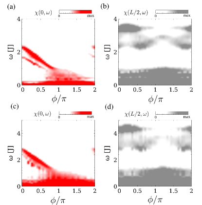
Figure 7: Dynamical structure factor $\chi(\omega)$ at the edge (a,c) and bulk (b,d) for a Harper-Heisenberg chain of Eq. (1), for spins $S=3/2$ (a,b) and $S=2$ (c,d). In particular, panels (b,d) show the emergence of a spectral gap in the bulk, that hosts pumping modes at the edge (a,c). This situation is analogous to the pumping shown for $S=1/2$ in Fig. 3, $S=1$ in Fig. 5 and ultimately, the free fermion case of Fig. 2. In comparison with the $S=1/2$ case of Fig. 3, a simple mapping with the free fermionic case of Fig. 2 can not be performed. We took $\alpha=\pi/\sqrt{2}$ and $\lambda=0.5$ for panels (a,b,c,d).

Previously, we focused on $S=1/2$ and $S=1$ chains, for which we showed the emergence of topological pumping modes. We turn to study whether such physics survives for higher-spin superlattice chains, and optimally, whether a large-$S$ limit could be identified.Gozel et al. (2018) Towards answering this question, we now study the case of topological pumps for the $S=3/2$ and $S=2$ Heisenberg superlattice models, following an analogous procedure as the one highlighted in the previous section.

We first point out several features of the large-$S$ limit: the physics of large-$S$ spin chains resembles in certain aspects the semiclassical limit. This can be qualitatively understood from the fact that the commutation relation of the $S_{\alpha}$ matrices become less relevant as the value of $S$ increases. In this regard, one could naively think that large-$S$ Heisenberg models would approach a classical limit with symmetry breaking, hosting a Néel order. This is, however, not the case, as large-$S$ Heisenberg chains still retain a singlet ground state with no symmetry breaking, and thus their ground state must be treated within a many-body framework.Xavier (2010) In particular, according to Haldane’s conjecture for integer $S$, the ground state of a uniform Heisenberg model is expected to host a finite gap whereas for half-integer it is expected to be gapless, which has been verified for $S=1/2$,Alcaraz et al. (1988); Luther and Peschel (1975), $S=1$,Golinelli et al. (1994); White (1992) $S=3/2$Ziman and Schulz (1987); Hallberg et al. (1996) and $S=2$.Granroth et al. (1996); Nishiyama et al. (1995); Wang et al. (1999)

We consider the Heisenberg superlatttice chains of higher spin, focusing on $S=3/2$ and $S=2$ cases. We show in Fig. 7 the bulk and edge spectra as a function of the pumping parameter $\phi$ for an $S=3/2$ and an $S=2$ spin chain, which again show the emergence of boundary pumping edge excitations in bulk spectral gaps. In particular, we observe that the spectra for $S=3/2$ and $S=2$ are qualitatively similar apart from an overall bandwidth increase. The bandwidth increase can be understood in terms of an increase in the spin stiffness arising from the higher spin of the chain. The similarity in the spectra suggests that the system is reaching a large-$S$ limit, implying that the topological pumping states are a generic feature of modulated quantum spin chains.

IV Conclusion

We have shown that quantum spin superlattice chains host topological excitations originating from the mapping of the superlattice to a topological pump. Specifically, we have shown that the emergence of such boundary modes in $S=1/2$ chains can be understood using a continuous deformation into a free-particle superlattice, where the 1D topological pump and its boundary modes are equivalent to a scan over the physics of the integer 2D quantum Hall state. The fact that we can perform this deformation between the 1D interacting Heisenberg model and the 1D free-fermion case demonstrates that at excitation gaps that do not close, the boundary in-gap excitations share the same topological origin. Such a deformation is verified numerically, showing bulk spectral gaps that do not close as one adiabatically goes from the free fermion limit to the Heisenberg limit. This is a first strong indication that the geometrical lengthscale competition leading to nontrivial topology in single-particle models, carries on to the many-body world. Crucially, we have shown that the very same topological boundary excitations appear in higher-$S$ spin chains, suggesting that the emergence of topological boundary modes is a generic feature of superlattice Hamiltonians, even when an adiabatic connection to a free-particle model is not known.

Our findings have several important consequences: (i) our results motivate possible further extensions of topological characterization to superlattice many-body systems and their excitation gaps; (ii) we show that long-ranged spatial modulations in many-body 1D systems provide a platform to study topological effects and their interplay with other many-body effects, such as critical exponent and many-body localization; (iii) our results highlight that modulated Heisenberg systems provide a compelling framework to explore the interplay of topological pumping excitations and quantum magnetism; and (iv) using contemporary numerical methods, we can explore a whole new range of many-body phenomena corresponding to excitations far above common low-energy treatments.

References

- Qi and Zhang (2011) X.-L. Qi and S.-C. Zhang, Rev. Mod. Phys. 83, 1057 (2011).
- Hasan and Kane (2010) M. Z. Hasan and C. L. Kane, Rev. Mod. Phys. 82, 3045 (2010).
- Su et al. (1979) W. P. Su, J. R. Schrieffer, and A. J. Heeger, Phys. Rev. Lett. 42, 1698 (1979).
- Avron et al. (1988) J. E. Avron, L. Sadun, J. Segert, and B. Simon, Phys. Rev. Lett. 61, 1329 (1988).
- Kane and Mele (2005) C. L. Kane and E. J. Mele, Phys. Rev. Lett. 95, 226801 (2005).
- Qi et al. (2008) X.-L. Qi, T. L. Hughes, and S.-C. Zhang, Phys. Rev. B 78, 195424 (2008).
- Fu (2011) L. Fu, Phys. Rev. Lett. 106, 106802 (2011).
- Chiu et al. (2016) C.-K. Chiu, J. C. Y. Teo, A. P. Schnyder, and S. Ryu, Rev. Mod. Phys. 88, 035005 (2016).
- Ozawa et al. (2019) T. Ozawa, H. M. Price, A. Amo, N. Goldman, M. Hafezi, L. Lu, M. C. Rechtsman, D. Schuster, J. Simon, O. Zilberberg, and I. Carusotto, Rev. Mod. Phys. 91, 015006 (2019).
- Cooper et al. (2019) N. R. Cooper, J. Dalibard, and I. B. Spielman, Rev. Mod. Phys. 91, 015005 (2019).
- Lu et al. (2009) M.-H. Lu, L. Feng, and Y.-F. Chen, Materials Today 12, 34 (2009).
- Serra-Garcia et al. (2018) M. Serra-Garcia, V. Peri, R. Süsstrunk, O. R. Bilal, T. Larsen, L. G. Villanueva, and S. D. Huber, Nature 555, 342 (2018).
- Brendel et al. (2018) C. Brendel, V. Peano, O. Painter, and F. Marquardt, Phys. Rev. B 97, 020102 (2018).
- Süsstrunk and Huber (2015) R. Süsstrunk and S. D. Huber, Science 349, 47 (2015).
- Albert et al. (2015) V. V. Albert, L. I. Glazman, and L. Jiang, Phys. Rev. Lett. 114, 173902 (2015).
- Ningyuan et al. (2015) J. Ningyuan, C. Owens, A. Sommer, D. Schuster, and J. Simon, Phys. Rev. X 5, 021031 (2015).
- Imhof et al. (2018) S. Imhof, C. Berger, F. Bayer, J. Brehm, L. W. Molenkamp, T. Kiessling, F. Schindler, C. H. Lee, M. Greiter, T. Neupert, and R. Thomale, Nature Physics 14, 925 (2018).
- Koch et al. (2010) J. Koch, A. A. Houck, K. L. Hur, and S. M. Girvin, Phys. Rev. A 82, 043811 (2010).
- Thouless et al. (1982) D. J. Thouless, M. Kohmoto, M. P. Nightingale, and M. den Nijs, Phys. Rev. Lett. 49, 405 (1982).
- Thouless (1983) D. J. Thouless, Phys. Rev. B 27, 6083 (1983).
- Kraus et al. (2012) Y. E. Kraus, Y. Lahini, Z. Ringel, M. Verbin, and O. Zilberberg, Phys. Rev. Lett. 109, 106402 (2012).
- Lohse et al. (2016) M. Lohse, C. Schweizer, O. Zilberberg, M. Aidelsburger, and I. Bloch, Nature Physics 12, 350 (2016).
- Lohse et al. (2018) M. Lohse, C. Schweizer, H. M. Price, O. Zilberberg, and I. Bloch, Nature 553, 55 (2018).
- Zilberberg et al. (2018) O. Zilberberg, S. Huang, J. Guglielmon, M. Wang, K. Chen, Y. E. Kraus, and M. C. Rechtsman, Nature 553, 59 (2018).
- Lang et al. (2012) L.-J. Lang, X. Cai, and S. Chen, Phys. Rev. Lett. 108, 220401 (2012).
- Kraus and Zilberberg (2012) Y. E. Kraus and O. Zilberberg, Phys. Rev. Lett. 109, 116404 (2012).
- Kraus et al. (2013) Y. E. Kraus, Z. Ringel, and O. Zilberberg, Phys. Rev. Lett. 111, 226401 (2013).
- Verbin et al. (2015) M. Verbin, O. Zilberberg, Y. Lahini, Y. E. Kraus, and Y. Silberberg, Phys. Rev. B 91, 064201 (2015).
- Kraus and Zilberberg (2016) Y. E. Kraus and O. Zilberberg, Nature Physics 12, 624 (2016).
- Senthil (2015) T. Senthil, Annual Review of Condensed Matter Physics 6, 299 (2015).
- Aidelsburger et al. (2014) M. Aidelsburger, M. Lohse, C. Schweizer, M. Atala, J. T. Barreiro, S. Nascimbène, N. R. Cooper, I. Bloch, and N. Goldman, Nature Physics 11, 162 (2014).
- Boada et al. (2015) O. Boada, A. Celi, J. Rodríguez-Laguna, J. I. Latorre, and M. Lewenstein, New Journal of Physics 17, 045007 (2015).
- Mancini et al. (2015) M. Mancini, G. Pagano, G. Cappellini, L. Livi, M. Rider, J. Catani, C. Sias, P. Zoller, M. Inguscio, M. Dalmonte, and L. Fallani, Science 349, 1510 (2015).
- Stuhl et al. (2015) B. K. Stuhl, H.-I. Lu, L. M. Aycock, D. Genkina, and I. B. Spielman, Science 349, 1514 (2015).
- Li et al. (2016) T. Li, L. Duca, M. Reitter, F. Grusdt, E. Demler, M. Endres, M. Schleier-Smith, I. Bloch, and U. Schneider, Science 352, 1094 (2016).
- Goldman et al. (2016) N. Goldman, J. C. Budich, and P. Zoller, Nature Physics 12, 639 (2016).
- Viebahn et al. (2019) K. Viebahn, M. Sbroscia, E. Carter, J.-C. Yu, and U. Schneider, Phys. Rev. Lett. 122, 110404 (2019).
- Choi et al. (2019) D.-J. Choi, N. Lorente, J. Wiebe, K. von Bergmann, A. F. Otte, and A. J. Heinrich, arXiv e-prints , arXiv:1904.09941 (2019), arXiv:1904.09941 [cond-mat.mes-hall] .
- Loth et al. (2012) S. Loth, S. Baumann, C. P. Lutz, D. M. Eigler, and A. J. Heinrich, Science 335, 196 (2012).
- Otte et al. (2008) A. F. Otte, M. Ternes, K. von Bergmann, S. Loth, H. Brune, C. P. Lutz, C. F. Hirjibehedin, and A. J. Heinrich, Nature Physics 4, 847 (2008).
- Choi et al. (2017) D.-J. Choi, R. Robles, S. Yan, J. A. J. Burgess, S. Rolf-Pissarczyk, J.-P. Gauyacq, N. Lorente, M. Ternes, and S. Loth, Nano Letters 17, 6203 (2017).
- von Bergmann et al. (2015) K. von Bergmann, M. Ternes, S. Loth, C. P. Lutz, and A. J. Heinrich, Phys. Rev. Lett. 114, 076601 (2015).
- Toskovic et al. (2016) R. Toskovic, R. van den Berg, A. Spinelli, I. S. Eliens, B. van den Toorn, B. Bryant, J.-S. Caux, and A. F. Otte, Nature Physics 12, 656 (2016).
- Spinelli et al. (2014) A. Spinelli, B. Bryant, F. Delgado, J. Fernández-Rossier, and A. F. Otte, Nature Materials 13, 782 (2014).
- Bryant et al. (2015) B. Bryant, R. Toskovic, A. Ferrón, J. L. Lado, A. Spinelli, J. Fernández-Rossier, and A. F. Otte, Nano Letters 15, 6542 (2015).
- Yang et al. (2017) K. Yang, Y. Bae, W. Paul, F. D. Natterer, P. Willke, J. L. Lado, A. Ferrón, T. Choi, J. Fernández-Rossier, A. J. Heinrich, and C. P. Lutz, Phys. Rev. Lett. 119, 227206 (2017).
- Baumann et al. (2015) S. Baumann, W. Paul, T. Choi, C. P. Lutz, A. Ardavan, and A. J. Heinrich, Science 350, 417 (2015).
- Natterer et al. (2017) F. D. Natterer, K. Yang, W. Paul, P. Willke, T. Choi, T. Greber, A. J. Heinrich, and C. P. Lutz, Nature 543, 226 (2017).
- Yazyev (2010) O. V. Yazyev, Reports on Progress in Physics 73, 056501 (2010).
- Gonzalez-Herrero et al. (2016) H. Gonzalez-Herrero, J. M. Gomez-Rodriguez, P. Mallet, M. Moaied, J. J. Palacios, C. Salgado, M. M. Ugeda, J.-Y. Veuillen, F. Yndurain, and I. Brihuega, Science 352, 437 (2016).
- Brihuega and Yndurain (2017) I. Brihuega and F. Yndurain, The Journal of Physical Chemistry B 122, 595 (2017).
- Ramires and Lado (2019) A. Ramires and J. L. Lado, Phys. Rev. B 99, 245118 (2019).
- Crowley et al. (2018) P. J. D. Crowley, A. Chandran, and C. R. Laumann, Phys. Rev. Lett. 120, 175702 (2018).
- Vidal et al. (1999) J. Vidal, D. Mouhanna, and T. Giamarchi, Phys. Rev. Lett. 83, 3908 (1999).
- Hida (2001) K. Hida, Phys. Rev. Lett. 86, 1331 (2001).
- Vidal et al. (2001) J. Vidal, D. Mouhanna, and T. Giamarchi, Phys. Rev. B 65, 014201 (2001).
- Vieira (2005a) A. P. Vieira, Phys. Rev. B 71, 134408 (2005a).
- Arlego (2002) M. Arlego, Phys. Rev. B 66, 052419 (2002).
- Vieira (2005b) A. P. Vieira, Phys. Rev. Lett. 94, 077201 (2005b).
- Arlego et al. (2001) M. Arlego, D. C. Cabra, and M. D. Grynberg, Phys. Rev. B 64, 134419 (2001).
- Roux et al. (2013) G. Roux, A. Minguzzi, and T. Roscilde, New Journal of Physics 15, 055003 (2013).
- Roux et al. (2008) G. Roux, T. Barthel, I. P. McCulloch, C. Kollath, U. Schollwöck, and T. Giamarchi, Phys. Rev. A 78, 023628 (2008).
- Kraus et al. (2014) Y. E. Kraus, O. Zilberberg, and R. Berkovits, Phys. Rev. B 89, 161106 (2014).
- Vieira and Hoyos (2018) A. P. Vieira and J. A. Hoyos, Phys. Rev. B 98, 104203 (2018).
- Friedman and Berkovits (2015) B.-e. Friedman and R. Berkovits, Phys. Rev. B 91, 104203 (2015).
- Setiawan et al. (2017) F. Setiawan, D.-L. Deng, and J. H. Pixley, Phys. Rev. B 96, 104205 (2017).
- Mastropietro (2015) V. Mastropietro, Phys. Rev. Lett. 115, 180401 (2015).
- Iyer et al. (2013) S. Iyer, V. Oganesyan, G. Refael, and D. A. Huse, Phys. Rev. B 87, 134202 (2013).
- Weiße et al. (2006) A. Weiße, G. Wellein, A. Alvermann, and H. Fehske, Rev. Mod. Phys. 78, 275 (2006).
- (70) “Itensor,” http://itensor.org/.
- Hu et al. (2014) H. Hu, C. Cheng, Z. Xu, H.-G. Luo, and S. Chen, Phys. Rev. B 90, 035150 (2014).
- Hu et al. (2015) H.-P. Hu, C. Cheng, H.-G. Luo, and S. Chen, Scientific Reports 5 (2015), 10.1038/srep08433.
- Wessel et al. (2003) S. Wessel, A. Jagannathan, and S. Haas, Phys. Rev. Lett. 90, 177205 (2003).
- Hida (2004) K. Hida, Phys. Rev. Lett. 93, 037205 (2004).
- Lopez-Bezanilla and Lado (2019) A. Lopez-Bezanilla and J. L. Lado, Phys. Rev. Materials 3, 084003 (2019).
- Faddeev (1996) L. D. Faddeev, arXiv e-prints , hep-th/9605187 (1996), arXiv:hep-th/9605187 [hep-th] .
- Note (1) Dynamical responses in the different sites of the chain that are not averaged over are denoted with the color scheme of Fig. 1(c).
- Giamarchi (2003) T. Giamarchi, Quantum Physics in One Dimension (Oxford University Press, 2003).
- Harper (1955) P. G. Harper, Proceedings of the Physical Society. Section A 68, 874 (1955).
- Hatsugai (1993) Y. Hatsugai, Phys. Rev. Lett. 71, 3697 (1993).
- Mei et al. (2019) F. Mei, G. Chen, N. Goldman, L. Xiao, and S. Jia, arXiv e-prints , arXiv:1905.04549 (2019), arXiv:1905.04549 [cond-mat.quant-gas] .
- Peierls (1933) R. Peierls, Zeitschrift f r Physik 80, 763 (1933).
- Xiao et al. (2010) D. Xiao, M.-C. Chang, and Q. Niu, Rev. Mod. Phys. 82, 1959 (2010).
- Soluyanov and Vanderbilt (2011) A. A. Soluyanov and D. Vanderbilt, Phys. Rev. B 83, 035108 (2011).
- Schulz-Baldes et al. (1999) H. Schulz-Baldes, J. Kellendonk, and T. Richter, Journal of Physics A: Mathematical and General 33, L27 (1999).
- KELLENDONK et al. (2002) J. KELLENDONK, T. RICHTER, and H. SCHULZ-BALDES, Reviews in Mathematical Physics 14, 87 (2002).
- Klitzing et al. (1980) K. v. Klitzing, G. Dorda, and M. Pepper, Phys. Rev. Lett. 45, 494 (1980).
- Avron et al. (2000) J. E. Avron, A. Elgart, G. M. Graf, and L. Sadun, Phys. Rev. B 62, R10618 (2000).
- Hofstadter (1976) D. R. Hofstadter, Phys. Rev. B 14, 2239 (1976).
- Chang and Niu (1995) M.-C. Chang and Q. Niu, Phys. Rev. Lett. 75, 1348 (1995).
- Note (2) Spectral functions averaged over will be denoted with the same color scheme as Fig. 2(c).
- Note (3) The MPS-KPM algorithm can be performed with a Hamiltonian whose full spectrum is scaled and shifted to fit the interval , which for computational efficiently should be done in with the spectral center located at 0.
- Jackson (1912) D. Jackson, Transactions of the American Mathematical Society 13, 491 (1912).
- White (1992) S. R. White, Phys. Rev. Lett. 69, 2863 (1992).
- Schollwöck (2005) U. Schollwöck, Rev. Mod. Phys. 77, 259 (2005).
- Stoudenmire and White (2013) E. M. Stoudenmire and S. R. White, Phys. Rev. B 87, 155137 (2013).
- (97) “dmrgpy,” https://github.com/joselado/dmrgpy.
- Wolf et al. (2014) F. A. Wolf, I. P. McCulloch, O. Parcollet, and U. Schollwöck, Phys. Rev. B 90, 115124 (2014).
- Wolf et al. (2015) F. A. Wolf, J. A. Justiniano, I. P. McCulloch, and U. Schollwöck, Phys. Rev. B 91, 115144 (2015).
- Halimeh et al. (2015) J. C. Halimeh, F. Kolley, and I. P. McCulloch, Phys. Rev. B 92, 115130 (2015).
- Ganahl et al. (2014) M. Ganahl, P. Thunström, F. Verstraete, K. Held, and H. G. Evertz, Phys. Rev. B 90, 045144 (2014).
- (102) V. Mastropietro, http://arxiv.org/abs/1811.11868v1 .
- Mastropietro (2016) V. Mastropietro, Phys. Rev. B 93, 245154 (2016).
- Apalkov and Chakraborty (2014) V. M. Apalkov and T. Chakraborty, Phys. Rev. Lett. 112, 176401 (2014).
- Gozel et al. (2018) S. Gozel, F. Mila, and I. Affleck, arXiv e-prints , arXiv:1810.02626 (2018), arXiv:1810.02626 [cond-mat.str-el] .
- Xavier (2010) J. C. Xavier, Phys. Rev. B 81, 224404 (2010).
- Alcaraz et al. (1988) F. C. Alcaraz, M. N. Barber, and M. T. Batchelor, Annals of Physics 182, 280 (1988).
- Luther and Peschel (1975) A. Luther and I. Peschel, Phys. Rev. B 12, 3908 (1975).
- Golinelli et al. (1994) O. Golinelli, T. Jolicoeur, and R. Lacaze, Phys. Rev. B 50, 3037 (1994).
- Ziman and Schulz (1987) T. Ziman and H. J. Schulz, Phys. Rev. Lett. 59, 140 (1987).
- Hallberg et al. (1996) K. Hallberg, X. Q. G. Wang, P. Horsch, and A. Moreo, Phys. Rev. Lett. 76, 4955 (1996).
- Granroth et al. (1996) G. E. Granroth, M. W. Meisel, M. Chaparala, T. Jolicœur, B. H. Ward, and D. R. Talham, Phys. Rev. Lett. 77, 1616 (1996).
- Nishiyama et al. (1995) Y. Nishiyama, K. Totsuka, N. Hatano, and M. Suzuki, Journal of the Physical Society of Japan 64, 414 (1995).
- Wang et al. (1999) X. Wang, S. Qin, and L. Yu, Phys. Rev. B 60, 14529 (1999).