Abstract

The $B$ meson semileptonic modes to $\rho(770)$ and $a_{1}(1260)$ are useful to pin down possible non Standard Model effects. The 4d differential $\bar{B}\to\rho(\pi\pi)\ell^{-}\bar{\nu}_{\ell}$ and $\bar{B}\to a_{1}(\rho\pi)\ell^{-}\bar{\nu}_{\ell}$ decay distributions are computed in SM and in extensions involving new Lepton Flavour Universality violating semileptonic $b\to u$ operators. The Large Energy limit for the light meson is also considered for both modes. The new effective couplings are constrained using the available data, and several observables in $\bar{B}\to\rho(\pi\pi)\ell^{-}\bar{\nu}_{\ell}$ in which NP effects can be better identified are selected, using the angular coefficient functions. The complementary role of $\bar{B}\to\rho(\pi\pi)\ell^{-}\bar{\nu}_{\ell}$ and $\bar{B}\to a_{1}(\rho\pi)\ell^{-}\bar{\nu}_{\ell}$ is discussed.

1 Introduction

The anomalies recently emerged in the flavour sector challenge both the experimental analyses and the theoretical interpretations. In the tree-level $b\to c\ell^{-}\bar{\nu}_{\ell}$ process, deviations of the ratios $\displaystyle R(D^{(*)})=\frac{{\cal B}(B\to D^{(*)}\tau^{-}{\bar{\nu}}_{\tau})}{{\cal B}(B\to D^{(*)}\ell^{-}{\bar{\nu}}_{\ell})}$ (with $\ell=e,\mu$) from the Standard Model (SM) expectations have been observed by BABAR [1, 2], Belle [3, 4, 5, 6] and LHCb [7, 8, 9]. The measurements can be summarized as $R(D)_{exp}=0.407\pm 0.039\pm 0.024$ to be combined with the new Belle result $R(D)_{exp}=0.307\pm 0.037\pm 0.016$ [10], and $R(D^{*})_{exp}=0.295\pm 0.011\pm 0.008$. These measurements are $3.1\,\sigma$ away from the SM values quoted by the Heavy Flavour Averaging Group (HFLAV) [11]: $R(D)_{SM}=0.299\pm 0.003$ and $R(D^{*})_{SM}=0.258\pm 0.005$. The tension, noticed in [12], is significant since the hadronic uncertainties largely cancel out in the ratios of branching fractions [13]. The LHCb measurement $\displaystyle R(J/\psi)=\displaystyle\frac{{\cal B}(B_{c}^{+}\to J/\psi\tau^{+}\nu_{\tau})}{{\cal B}(B_{c}^{+}\to J/\psi\mu^{+}\nu_{\mu})}=0.71\pm 0.17({\rm stat})\pm 0.18({\rm syst})$ [14] also exceeds the SM expectation, however in these modes the hadronic uncertainties are sizable [15, 16, 17].

Other anomalies have been detected in neutral current $b\to s$ semileptonic transitions, in the ratios $\displaystyle R_{K^{(*)}}=\frac{\int_{q^{2}_{min}}^{q^{2}_{max}}\frac{d\Gamma}{dq^{2}}(B^{+}\to K^{(*)}\mu^{+}\mu^{-})dq^{2}}{\int_{q^{2}_{min}}^{q^{2}_{max}}\frac{d\Gamma}{dq^{2}}(B^{+}\to K^{(*)}e^{+}e^{-})dq^{2}}$ measured by LHCb and Belle. The updated result for $R_{K}$ is $\displaystyle R_{K^{+}}=0.846^{+0.060}_{-0.054}({\rm stat})^{-0.016}_{-0.014}({\rm syst})$ for $[q^{2}_{min},q^{2}_{max}]=[1.1\,{\rm GeV}^{2},6\,{\rm GeV}^{2}]$ [18]. For $R_{K^{*}}$, the measurements $\displaystyle R_{K^{*0}}=0.66\pm^{0.11}_{0.07}({\rm stat})\pm 0.03({\rm syst})$ for $q^{2}$ in $[0.045\,{\rm GeV}^{2},1.1\,{\rm GeV}^{2}]$ and $\displaystyle R_{K^{*0}}=0.69\pm^{0.11}_{0.07}({\rm stat})\pm 0.05({\rm syst})$ for $q^{2}$ in $[1.1\,{\rm GeV}^{2},6\,{\rm GeV}^{2}]$ have been reported by LHCb [19]. Recent Belle measurements, averaged over the neutral and charged modes, are affected by larger errors: $\displaystyle R_{K^{*}}=0.52\pm^{0.36}_{0.26}({\rm stat})\pm 0.05({\rm syst})$ for $q^{2}$ in $[0.045\,{\rm GeV}^{2},1.1\,{\rm GeV}^{2}]$, $\displaystyle R_{K^{*}}=0.90\pm^{0.27}_{0.21}({\rm stat})\pm 0.10({\rm syst})$ for $q^{2}$ in $[0.1\,{\rm GeV}^{2},8\,{\rm GeV}^{2}]$, and $\displaystyle R_{K^{*}}=1.18\pm^{0.52}_{0.32}({\rm stat})\pm 0.10({\rm syst})$ for $q^{2}$ in $[15\,{\rm GeV}^{2},19\,{\rm GeV}^{2}]$ [20]. For all the ratios the SM predictions are close to one.

The anomalies in $b\to c$ and $b\to s$ semileptonic modes seem to point to violation of lepton flavour universality (LFU). This accidental SM symmetry is only broken by the Yukawa interactions, while the lepton couplings to the gauge bosons are independent of the lepton flavour. It is unclear if the deviations emerged in angular observables in $B\to K^{*}\mu^{+}\mu^{-}$ [22, 23] and in the rate of $B_{s}^{0}\to\phi\mu^{+}\mu^{-}$ [24] can have a connected origin.

In addition to these tensions, the long-standing difference in the determination of the CKM matrix element $|V_{cb}|$ from exclusive modes, in particular $\bar{B}\to D^{*}\ell^{-}\bar{\nu}_{\ell}$, and from inclusive $\bar{B}\to X_{c}\ell^{-}\bar{\nu}_{\ell}$ observables (width and moments) still persists in new BABAR [25] and Belle analyses [26], with $|V_{cb}|_{excl}<|V_{cb}|_{incl}$. As an alternative to solutions to the puzzle within SM [27, 28, 29, 30], a connection has been proposed with the other $b\to c$ anomalies, within a LFU violating framework [13, 31]. The related experimental signatures have been studied, in particular the 4d differential $\bar{B}\to D^{*}(D\pi,D\gamma)\ell^{-}\bar{\nu}_{\ell}$ decay distributions for the three lepton species have been scrutinized [32], following analyses that have pointed out the relevance of such distributions [33, 34, 35, 36].

It is worth wondering if similar deviations can appear in semileptonic $b\to u$ transitions. These modes are CKM suppressed with respect to the $b\to c$ ones, nevertheless high precision measurements are foreseen in the near future by LHCb and Belle II. At present, there is a tension between the exclusive measurement of $|V_{ub}|$, mainly from the $\bar{B}\to\pi\ell^{-}\bar{\nu}_{\ell}$ decay width, and the inclusive determination from $\bar{B}\to X_{u}\ell^{-}\bar{\nu}_{\ell}$ observables. New information is available on the purely leptonic and on the semileptonic $B\to\pi$ mode, and analyses within and beyond SM have been carried out [37, 38, 39, 40, 41, 42, 43, 44, 45].

Other decay modes can be exploited to pin down deviation from the Standard Model. In particular, for the modes involving the vector $\rho(770)$ and the axial-vector $a_{1}(1260)$ mesons, the fully differential angular distributions when $\rho$ decays in two pions and $a_{1}$ decays into $\rho\pi$ represent an important source of information, due to the wealth of observables that can be analyzed. Such observables are all correlated, and are able to provide coherent patterns within SM and its possible extensions. The different parity of the two mesons acts as a filter for NP operators, which is one of the prime motivations for their consideration. In addition, the $a_{1}\to\rho\pi$ mode has the peculiarity that the longitudinal and tranverse $\rho$ polarizations are involved, increasing the plethora of observables on which to focus the experimental analyses. Our NP extension includes lepton-flavour dependent operators, and the comparison with the effects of corresponding $b\to c$ operators could sheld light on the structure of the observed LFU violating effects.

In Sect.2 we introduce the semileptonic $b\to u$ effective Hamiltonian with the inclusion of new scalar, pseudoscalar, vector and tensor operators weighted by complex couplings. Such operators affect the $\bar{B}$ transitions to two leptons and to $\pi\ell\bar{\nu}$, and both channels can be exploited to bound the effective coefficients. In Sect.3 we construct the fully differential decay distributions for the $\bar{B}\to\rho(\pi\pi)\ell^{-}\bar{\nu}_{\ell}$ and $\bar{B}\to a_{1}(\rho\pi)\ell^{-}\bar{\nu}_{\ell}$ modes, computing the sets of angular coefficient functions in terms of the hadronic matrix elements involved in the transitions. We also consider the Large Energy limit for the light mesons, which allows to express the angular functions in terms of a small number of hadronic form factors. In Sect.4 we analyze several observables in $\bar{B}\to\rho(\pi\pi)\ell^{-}\bar{\nu}_{\ell}$ at a benchmark point in the parameter space of the new couplings, to scrutinize their sensitivity to the different new operators. In particular, we focus on the angular coefficient functions and on combinations for which the new operators would exhibit the largest effect. In Sect.5 we elaborate on the $a_{1}(1260)$ mode: in such a case the uncertainties on the sets of hadronic form factors are large and still need to be precisely assessed. Nevertheless, we present a numerical analysis of a few observables, to show the sensitivity of the $a_{1}$ mode to NP, but the main focus is on the analytic results and on the outcome of the Large Energy limit, to explain the complementarity with the $\rho$ mode. The last Section contains a discussion of the interesting perspectives and the conclusions. In the Appendices we collect the definitions of the hadronic matrix elements and the expressions of the angular coefficient functions for the two modes.

2 Effective $b\to u\ell^{-}\bar{\nu}_{\ell}$ NP Hamiltonian and impact on $B$ meson purely leptonic and semileptonic pion modes

New Physics contributions to beauty hadron decays can be analysed within the Standard Model Effective Field Theory. If the NP scale $\Lambda_{NP}$ is much larger than the EW scale, all the new massive degrees of freedom can be integrated out, obtaining an effective Hamiltonian in which only the SM fields appear and which is invariant under the SM gauge group. This Hamiltonian contains additional operators with respect to SM, suppressed by increasing powers of $\Lambda_{NP}$. The contribution ${\cal O}\left(\displaystyle\frac{1}{\Lambda_{NP}^{2}}\right)$ includes dimension-six four-fermion operators [46].

To describe the modes ${\bar{B}}\to M_{u}\ell^{-}{\bar{\nu}}_{\ell}$ with $M_{u}$ a light meson comprising an up quark we consider the effective Hamiltonian

$$H_{\rm eff}^{b\to u\ell\nu}={G_{F}\over\sqrt{2}}V_{ub} \Big{\{} (1+\epsilon_{V}^{\ell})\left({\bar{u}}\gamma_{\mu}(1-\gamma_{5})b\right)\left({\bar{\ell}}\gamma^{\mu}(1-\gamma_{5}){\nu}_{\ell}\right)$$ (1)

$$+ \epsilon_{S}^{\ell}\,({\bar{u}}b)\left({\bar{\ell}}(1-\gamma_{5}){\nu}_{\ell}\right)+\epsilon_{P}^{\ell}\,\left({\bar{u}}\gamma_{5}b\right)\left({\bar{\ell}}(1-\gamma_{5}){\nu}_{\ell}\right)$$

$$+ \epsilon_{T}^{\ell}\,\left({\bar{u}}\sigma_{\mu\nu}(1-\gamma_{5})b\right)\,\left({\bar{\ell}}\sigma^{\mu\nu}(1-\gamma_{5}){\nu}_{\ell}\right)\Big{\}}+h.c.\,\,\,,$$

consisting in the SM term and in NP terms weighted by complex lepton-flavour dependent couplings $\epsilon^{\ell}_{V,S,P,T}$. $V_{ub}$ and $\epsilon_{V}^{\ell}$ are independent parameters, since the product $V_{ub}(1+\epsilon_{V}^{\ell})$ is not a mere redefinition of the SM $V_{ub}$. We assume a purely left-handed lepton current as in SM, an extensively probed structure. We exclude the quark right-handed vector current, since the only four-fermion operator of this type, invariant under the SM group, is non-linear in the Higgs field [47, 48, 49] .

The couplings of the NP operators in (1) are constrained by the measurements, in particular on the purely leptonic $B^{-}$ and semileptonic $\bar{B}\to\pi\ell^{-}\bar{\nu}_{\ell}$ channels. Indeed, the $B^{-}\to\ell^{-}\bar{\nu}_{\ell}$ decay width obtained from $H_{\rm eff}^{b\to u\ell\nu}$ in Eq.(1) reads

$$\Gamma(B^{-}\to\ell^{-}\bar{\nu}_{\ell})=\frac{G_{F}^{2}|V_{ub}|^{2}f_{B}^{2}m_{B}^{3}}{8\pi}\left(1-\frac{m_{\ell}^{2}}{m_{B}^{2}}\right)^{2}\left|\left(\frac{m_{\ell}}{m_{B}}\right)(1+\epsilon_{V}^{\ell})+\frac{m_{B}}{m_{b}+m_{u}}\epsilon_{P}^{\ell}\right|^{2}\,\,,$$ (2)

with the decay constant $f_{B}$ defined as

$$\langle 0|{\bar{u}}\gamma_{\mu}\gamma_{5}b|{\bar{B}}(p)\rangle=i\,f_{B}p_{\mu}\,\,\,.$$ (3)

The ew correction to (2) is tiny. This mode is insensitive to the NP scalar and tensor operators. The pseudoscalar operator removes the helicity suppression, which is effective for light leptons, with a consequent stringent constraint for the effective couplings $\epsilon_{P}^{e,\,\mu}$.

The semileptonic $\bar{B}\to\pi\ell^{-}\bar{\nu}_{\ell}$ decay distribution in the dilepton mass squared $q^{2}$, obtained from Eq.(1) parametrizing the weak matrix element in terms of the form factors $f_{i}(q^{2})=f_{i}^{B\to\pi}(q^{2})$ as in Appendix A, is:

$$\frac{d\Gamma}{dq^{2}}(\bar{B}\to\pi\ell^{-}\bar{\nu}_{\ell}) = \frac{G_{F}^{2}|V_{ub}|^{2}\lambda^{1/2}(m_{B}^{2},m_{\pi}^{2},q^{2})}{128m_{B}^{3}\pi^{3}q^{2}}\left(1-\frac{m_{\ell}^{2}}{q^{2}}\right)^{2}$$

$$\times \Bigg{\{}\left|m_{\ell}(1+\epsilon_{V}^{\ell})+\frac{q^{2}\epsilon_{S}^{\ell}}{m_{b}-m_{u}}\right|^{2}(m_{B}^{2}-m_{\pi}^{2})^{2}f_{0}^{2}(q^{2})+$$

$$+ \lambda(m_{B}^{2},m_{\pi}^{2},q^{2})\Bigg{[}\frac{1}{3}\left|m_{\ell}(1+\epsilon_{V}^{\ell})f_{+}(q^{2})+\frac{4q^{2}}{m_{B}+m_{\pi}}\epsilon_{T}^{\ell}f_{T}(q^{2})\right|^{2}$$

$$+ \frac{2q^{2}}{3}\left|(1+\epsilon_{V}^{\ell})f_{+}(q^{2})+4\frac{m_{\ell}}{m_{B}+m_{\pi}}\epsilon_{T}^{\ell}f_{T}(q^{2})\right|^{2}\Bigg{]}\Bigg{\}}\,\,\,,$$

with $\lambda$ the triangular function. In this case the pseudoscalar operator does not contribute.

As in the Hamiltonian (1), in Eqs.(2) and (2) the CKM matrix element $V_{ub}$ appears in the combination $V_{ub}(1+\epsilon_{V}^{\ell})$. The lepton-flavour dependence of the effective couplings would manifest in different determinations of $V_{ub}$ from channels involving different lepton species. We discuss below how the experimental measurements constrain the parameter spaces.

Continuing with the semileptonic mode to pion, in the large energy limit of the emitted pion, using Eq.(A.13) for the weak matrix element, the decay distribution is expressed in terms of a single form factor $\xi_{\pi}$ [50, 51]:

$$\frac{d\Gamma}{dE}(\bar{B}\to\pi\ell^{-}\bar{\nu}_{\ell}) = \frac{G_{F}^{2}|V_{ub}|^{2}\lambda^{1/2}(m_{B}^{2},m_{\pi}^{2},q^{2})}{64m_{B}^{2}\pi^{3}q^{2}}\left(1-\frac{m_{\ell}^{2}}{q^{2}}\right)^{2}\xi_{\pi}^{2}(E)$$

$$\times \Bigg{\{}\left|m_{\ell}(1+\epsilon_{V}^{\ell})+\frac{q^{2}\epsilon_{S}^{\ell}}{m_{b}-m_{u}}\right|^{2}(m_{B}^{2}-m_{\pi}^{2})^{2}\left(\frac{m_{B}^{2}+m_{\pi}^{2}-q^{2}}{m_{B}^{2}}\right)^{2}$$

$$+ \lambda(m_{B}^{2},m_{\pi}^{2},q^{2})\Bigg{[}\frac{1}{3}\left|m_{\ell}(1+\epsilon_{V}^{\ell})+\frac{4q^{2}}{m_{B}}\epsilon_{T}^{\ell}\right|^{2}+\frac{2q^{2}}{3}\left|(1+\epsilon_{V}^{\ell})+\frac{4m_{\ell}}{m_{B}}\epsilon_{T}^{\ell}\right|^{2}\Bigg{]}\Bigg{\}},$$

with $q^{2}=m_{B}^{2}+m_{\pi}^{2}-2m_{B}E$. While the full kinematical range for $E$ is $m_{\pi}\leq E\leq\frac{m_{B}}{2}\left(1+\frac{m_{\pi}^{2}}{m_{B}^{2}}-\frac{m_{\ell}^{2}}{m_{B}^{2}}\right)$, Eq.(2) only holds for large $E\simeq\frac{m_{B}}{2}$. This expression is useful if the distribution is independently measured for the three charged leptons, since the ratios

$$\frac{dR(\pi)^{\ell\ell^{\prime}}}{dE}=\frac{d\Gamma}{dE}(\bar{B}\to\pi\ell^{-}\bar{\nu}_{\ell})/\frac{d\Gamma}{dE}(\bar{B}\to\pi\ell^{\prime-}\bar{\nu}_{\ell^{\prime}})$$ (6)

are free of hadronic uncertainties in this limit, and only involve combinations of the lepton flavour-dependent couplings $\epsilon_{V,S,T}^{\ell,\ell^{\prime}}$.

3 Fully differential angular distributions for $\bar{B}\to\rho(\to\pi\pi)\ell^{-}\bar{\nu}_{\ell}$ and $\bar{B}\to a_{1}(\to\rho\pi)\ell^{-}\bar{\nu}_{\ell}$

The main sensitivity to the new operators in (1), in the modes $\bar{B}\to\rho(\to\pi\pi)\ell^{-}\bar{\nu}_{\ell}$ and $\bar{B}\to a_{1}(\to\rho\pi)\ell^{-}\bar{\nu}_{\ell}$, is in the 4d differential decay distribution in the variables $q^{2}$ and in the angles $\theta$, $\theta_{V}$ and $\phi$ described in Fig.1.

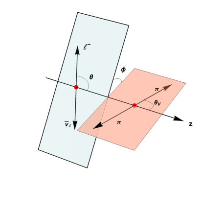
Figure 1: Kinematics of the decay mode $\bar{B}\to\rho(\pi\pi)\ell^{-}\bar{\nu}_{\ell}$.

For the $\rho$ mode the distribution is written as :

$$\frac{d^{4}\Gamma(\bar{B}\to\rho(\to\pi\pi)\ell^{-}\bar{\nu}_{\ell})}{dq^{2}\,d\cos\theta\,d\phi\,d\cos\theta_{V}} = {\cal N_{\rho}}|{\vec{p}}_{\rho}|\left(1-\frac{m_{\ell}^{2}}{q^{2}}\right)^{2}\Big{\{}I_{1s}^{\rho}\,\sin^{2}\theta_{V}+I_{1c}^{\rho}\,\cos^{2}\theta_{V}$$

$$+ \left(I_{2s}^{\rho}\,\sin^{2}\theta_{V}+I_{2c}^{\rho}\,\cos^{2}\theta_{V}\right)\cos 2\theta$$

$$+ I_{3}^{\rho}\,\sin^{2}\theta_{V}\sin^{2}\theta\cos 2\phi+I_{4}^{\rho}\,\sin 2\theta_{V}\sin 2\theta\cos\phi$$

$$+ I_{5}^{\rho}\,\sin 2\theta_{V}\sin\theta\cos\phi+\left(I_{6s}^{\rho}\,\sin^{2}\theta_{V}+I_{6c}^{\rho}\,\cos^{2}\theta_{V}\right)\cos\theta$$

$$+ I_{7}^{\rho}\sin 2\theta_{V}\sin\theta\sin\phi\Big{\}}\,\,,$$

with ${\cal N}_{\rho}=\displaystyle{\frac{3G_{F}^{2}|V_{ub}|^{2}{\cal B}(\rho\to\pi\pi)}{128(2\pi)^{4}m_{B}^{2}}}$. This expression, together with the relation of the coefficient functions to the hadronic matrix elements, has been computed in the narrow width approximation, resulting in a factorization of the production and decay amplitude of the intermediate vector meson. The factorization is connected to the procedure adopted in the experimental analyses to select the contributions of the intermediate resonances [52]. A $\pi\pi$ contribution considered as an improvement of the narrow width approximation has been investigated through the computation of the $B\to\pi\pi$ matrix elements in the kinematical regime of small dipion invariant mass and large energy, concluding that it represents a small effect [56, 57, 58].

For the $a_{1}(\rho\pi)$ channel it is useful to provide the expressions for the modes where the final $\rho$ is transversely ($\rho_{\perp}$) or longitudinally ($\rho_{\parallel}$) polarized, as specified in Appendix B. The expression of the 4d distribution amplitude is:

$$\frac{d^{4}\Gamma(\bar{B}\to a_{1}(\to\rho_{\parallel(\perp)}\pi)\ell^{-}\bar{\nu}_{\ell})}{dq^{2}\,d\cos\theta\,d\phi\,d\cos\theta_{V}} = {\cal N}_{a_{1}}^{\parallel(\perp)}|{\vec{p}}_{a_{1}}|\left(1-\frac{m_{\ell}^{2}}{q^{2}}\right)^{2}\Big{\{}I_{1s,\parallel(\perp)}^{a_{1}}\,\sin^{2}\theta_{V}+I_{1c,\parallel(\perp)}^{a_{1}}\,(3+\cos 2\theta_{V})$$

$$+ \left(I_{2s,\parallel(\perp)}^{a_{1}}\,\sin^{2}\theta_{V}+I_{2c,\parallel(\perp)}^{a_{1}}\,(3+\cos 2\theta_{V})\right)\cos 2\theta$$

$$+ I_{3,\parallel(\perp)}^{a_{1}}\,\sin^{2}\theta_{V}\sin^{2}\theta\cos 2\phi+I_{4,\parallel(\perp)}^{a_{1}}\sin 2\theta_{V}\sin 2\theta\cos\phi$$

$$+ I_{5,\parallel(\perp)}^{a_{1}}\,\sin 2\theta_{V}\sin\theta\cos\phi$$

$$+ \left(I_{6s,\parallel(\perp)}^{a_{1}}\,\sin^{2}\theta_{V}+I_{6c,\parallel(\perp)}^{a_{1}}\,(3+\cos 2\theta_{V})\right)\cos\theta$$

$$+ I_{7,\parallel(\perp)}^{a_{1}}\sin 2\theta_{V}\sin\theta\sin\phi\Big{\}}\,\,\,,$$

with the subscripts $\perp,\parallel$ referring to the two $\rho$ polarizations. The coefficients ${\cal N}_{a_{1}}^{\parallel(\perp)}$ read: ${\cal N}_{a_{1}}^{\parallel(\perp)}=\displaystyle{\frac{3G_{F}^{2}|V_{ub}|^{2}{\cal B}(a_{1}\to\rho_{\parallel(\perp)}\pi)}{128(2\pi)^{4}m_{B}^{2}}}$. The separation of the $\rho$ polarizations is an experimental challenge, which is justified in view of the different sensitivity of the angular coefficient functions to the NP operators. The unpolarized case is recovered combining the expressions for the transverse and longitudinal $\rho$ polarization. The NWA has been adopted also for the computation of the distribution (3) with the derivation of the relations of the angular coefficient functions in terms of $B\to a_{1}$ matrix elements. This is a more debatable procedure than for the $\rho$ channel. Its motivation relies on the assumption that the experimental analyses can constrain the $\rho\pi$ invariant mass in a narrow range around the $a_{1}$ peak, separating the production and decay process of the intermediate resonance. Going beyond such a limit would require to consider the $\rho\pi$ invariant mass distribution, with the $B\to a_{1}$ form factors extrapolated to different values of such a mass, with uncontrolled uncertainties. On the other hand, considering the three pion final state would include contributions from several resonances of various spin-parity, affected in different ways from the NP operators when produced in semileptonic $B$ modes.

The angular coefficient functions $I^{\rho}_{i}$ and $I^{a1}_{i}$ in Eqs.(3) and (3) can be written as

$$I_{i} = |1+\epsilon_{V}|^{2}\,I_{i}^{SM}+|\epsilon_{X}|^{2}I_{i}^{NP,X}+|\epsilon_{T}|^{2}I_{i}^{NP,T}+2\,{\rm Re}\left[\epsilon_{X}(1+\epsilon_{V}^{*})\right]I_{i}^{INT,X}$$ (9)

$$+ 2\,{\rm Re}\left[\epsilon_{T}(1+\epsilon_{V}^{*})\right]I_{i}^{INT,T}+2\,{\rm Re}\left[\epsilon_{X}\epsilon_{T}^{*}\right]I_{i}^{INT,XT},\,\,\,\,\hskip 85.35826pt(i=1,\dots 6),\hskip 14.22636pt$$

$$I_{7} = 2\,{\rm Im}\left[\epsilon_{X}(1+\epsilon_{V}^{*})\right]I_{7}^{INT,X}+2\,{\rm Im}\left[\epsilon_{T}(1+\epsilon_{V}^{*})\right]I_{7}^{INT,T}+2\,{\rm Im}\left[\epsilon_{X}\epsilon_{T}^{*}\right]I_{7}^{INT,XT},$$

with $X=P$ in case of $\rho$, and $X=S$ in case of $a_{1}$. The coefficient functions $I_{i}^{SM}$, $I_{i}^{NP}$ and $I_{i}^{INT}$, expressed in terms of helicity amplitudes, are collected in Tables 2-9 of Appendix B, together with the relations of the helicity amplitudes to the hadron form factors.

Examining the angular coefficient functions and their expressions, several remarks are in order.

1. With the exception of $I_{7}$, all angular coefficient functions do not vanish in SM and are sensitive to $\epsilon_{V}$. Apart from such a dependence, we can identify structures useful to disentangle the effects of the other S, P and T operators. In $B\to\rho\ell{\bar{\nu}}_{\ell}$ the functions $I_{1s}^{\rho},\,I_{2s}^{\rho},\,I_{2c}^{\rho},\,I_{3}^{\rho},\,I_{4}^{\rho},\,I_{6s}^{\rho}$ do not depend on $\epsilon_{P}$, as it can be inferred from Table 3, and are sensitive only to the tensor operator. We denote these structures as belonging to set A, while set B comprises the remaining ones. An analogous situation occurs for the corresponding quantities in $B\to a_{1}(\rho_{\parallel}\pi)\ell{\bar{\nu}}_{\ell}$, which do not depend on $\epsilon_{S}$ (Table 6), while in $B\to a_{1}(\rho_{\perp}\pi)\ell{\bar{\nu}}_{\ell}$ the functions $I_{1c,\perp}^{a_{1}},\,I_{2s,\perp}^{a_{1}},\,I_{2c,\perp}^{a_{1}},\,I_{3,\perp}^{a_{1}},\,I_{4,\perp}^{a_{1}},\,I_{6c,\perp}^{a_{1}}$ are insensitive to the scalar operator (Table 7).

2. In the absence of the tensor operator, the $\rho$ and $a_{1}$ modes give complementary information on the pseudoscalar P (in the $\rho$ channel ) and scalar S (in $a_{1}$) operators, together with the purely leptonic mode (sensitive to P) and $B\to\pi$ mode (sensitive to S).

3. There are angular coefficient functions that depend only on the helicity amplitudes $H_{\pm}$, not on $H_{0}$ and $H_{t}$. These affect observables corresponding to the transversely polarized $W$, hence to transverse $\rho$ in $B\to\rho\ell{\bar{\nu}}_{\ell}$ and transverse $a_{1}$ in $B\to a_{1}\ell{\bar{\nu}}_{\ell}$. Such observables depend on $\epsilon_{T}$, not on $\epsilon_{P}$ (in the $\rho$ mode) or $\epsilon_{S}$ (in the $a_{1}$ mode).

4. In the Large Energy Limit of the light meson, the form factors parametrizing the $B\to\rho(a_{1})$ weak matrix elements can be written in terms of two form factors, $\xi_{\perp}^{\rho}(\xi_{\perp}^{a_{1}})$ and $\xi_{\parallel}^{\rho}(\xi_{\parallel}^{a_{1}})$ defined by the relations (A.14), (A.15). In this limit, several angular coefficients depend only on the form factor $\xi_{\perp}$, others involve both $\xi_{\perp}$ and $\xi_{\parallel}$. The coefficients depending only on $\xi_{\perp}^{\rho,a_{1}}(E)$ are:

   • in $B\to\rho(770)$ mode: $I_{1s}^{\rho},\,I_{2s}^{\rho},\,I_{3}^{\rho}$ and $I_{6s}^{\rho}$ ,

   • in $B\to a_{1}(1260)$ mode:
     for final $\rho$ longitudinally polarized, $I_{1s,\parallel}^{a_{1}},\,I_{2s,\parallel}^{a_{1}},\,I_{3,\parallel}^{a_{1}}$ and $I_{6s,\parallel}^{a_{1}}$ ,
     for $\rho$ transversely polarized, $I_{1c,\perp}^{a_{1}},\,I_{2c,\perp}^{a_{1}},\,I_{3,\perp}^{a_{1}}$ and $I_{6c,\perp}^{a_{1}}$ .

   When a single form factor is involved, ratios of coefficient functions are free of hadronic uncertainties (in the Large Energy Limit).

The conclusion is that, measuring the differential angular distribution and reconstructing the angular coefficient functions, it is possible to define sets of observables particularly sensitive to different NP terms in (1). This would allow to determine the new couplings $\epsilon_{i}^{\ell}$ and carry out tests, e.g., of LFU, comparing results obtained in the $\mu$ and $\tau$ modes.

4 Constraints on the effective couplings and $\bar{B}\to\rho\ell^{-}\bar{\nu}_{\ell}$ observables

We want to present examples of the possible effects of the NP operators in (1) in $\bar{B}\to\rho\ell^{-}\bar{\nu}_{\ell}$, identifying the most sensitive observables. For that, we constrain the space of the new couplings using the available data and a set of hadronic quantities. More precise experimental measurements or more accurate theoretical determinations of the hadronic quatities, when available in the future, will modify the ranges of the couplings, but the strategy and the overall picture we are presenting will remain valid.

The couplings $\epsilon_{V}^{\mu},\ \epsilon_{P}^{\mu},\,\epsilon_{T}^{\mu}$ are constrained by the measurements ${\cal B}(\bar{B}^{0}\to\pi^{+}\ell^{-}{\bar{\nu}}_{\ell})=(1.50\pm 0.06)\times 10^{-4}$ and ${\cal B}(\bar{B}^{0}\to\rho^{+}\ell^{-}{\bar{\nu}}_{\ell})=(2.94\pm 0.21)\,10^{-4}$ [59], together with ${\cal B}(B^{-}\to\mu^{-}\bar{\nu}_{\mu})=(6.46\pm 2.2\pm 1.60)\times 10^{-7}$ (and 90% probability interval $[2.0,10.7]\times 10^{-7}$) [60]. For $e$ and $\tau$, the results for the purely leptonic modes are ${\cal B}(B^{-}\to e^{-}\bar{\nu}_{e})<9.8\times 10^{-7}$ and ${\cal B}(B^{-}\to\tau^{-}\bar{\nu}_{\tau})=(1.09\pm 0.24)\times 10^{-4}$ [59]. The upper bound ${\cal B}(\bar{B}^{0}\to\pi^{+}\tau^{-}{\bar{\nu}}_{\tau})<2.5\times 10^{-4}$ has also been established [61]. We use the $B\to\pi$ form factors given in Appendix C, obtained interpolating the Light-Cone sum rule results at low $q^{2}$ computed in Refs.[62, 63] with the lattice QCD results at large values of $q^{2}$ averaged by HFLAG [64]. For the $B\to\rho$ transition we use the form factors in Ref.[65], which update previous Light-Cone sum rule computations [66] and extrapolate the low $q^{2}$ determination to the full kinematical range.

In the case of $\mu$, the parameter space for the NP couplings, displayed in Fig.2, is found imposing that the purely leptonic BR is in the range $[2.0,10.7]\times 10^{-7}$, and that the semileptonic $\bar{B}\to\pi$ and $\bar{B}\to\,\rho$ branching fractions are compatible within $2\sigma$ with measurement. The benchmark point shown in Fig.2 is chosen in the region of the smallest

$$\chi^{2}=\sum_{i}^{3}\left(\frac{{\cal B}^{th}_{i}-{\cal B}^{exp}_{i}}{\Delta{\cal B}^{exp}_{i}}\right)^{2}$$ (10)

for the three modes, varying $|V_{ub}|$ in $[3.5,\,4.4]\times 10^{-3}$. Specifically, in the region of smallest $\chi^{2}$ we have selected the points in the parameter space having $\epsilon_{V}^{\ell}=0$ and all the other $\epsilon_{A}^{\ell}\neq 0$, with $A=S,P,T$. Our benchmark point is the one minimizing $\chi^{2}$. We set $\epsilon_{V}^{\ell}=0$ to maximize the sensitivity to the other NP couplings.

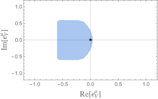
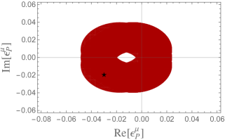
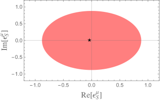
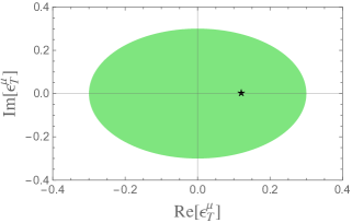
Figure 2: Allowed regions for the couplings $\epsilon_{V}^{\mu}$, $\epsilon_{P}^{\mu}$, $\epsilon_{S}^{\mu}$ and $\epsilon_{T}^{\mu}$. The colors distinguish the various couplings. The stars correspond to the benchmark points, chosen in the region of minimum $\chi^{2}$: $({\rm Re}[\epsilon_{V}^{\mu}],\,{\rm Im}[\epsilon_{V}^{\mu}])=(0,\,0)$, $({\rm Re}[\epsilon_{P}^{\mu}],\,{\rm Im}[\epsilon_{P}^{\mu}])=(-0.03,\,-0.02)$, $({\rm Re}[\epsilon_{T}^{\mu}],\,{\rm Im}[\epsilon_{T}^{\mu}])=(0.12,\,0)$ and $({\rm Re}[\epsilon_{S}^{\mu}],\,{\rm Im}[\epsilon_{S}^{\mu}])=(-0.04,\,0)$, with $|V_{ub}|=3.5\times 10^{-3}$.

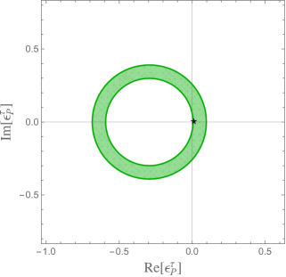
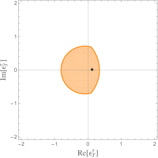
Figure 3: Allowed regions for the couplings $\epsilon_{P}^{\tau}$ and $\epsilon_{T}^{\tau}$. The stars correspond to the benchmark points chosen setting $\epsilon_{V}^{\tau}=0$ and $\epsilon_{S}^{\tau}=0$: $({\rm Re}[\epsilon_{P}^{\tau}],\,{\rm Im}[\epsilon_{P}^{\tau}])=(0.01,\,0)$ and $({\rm Re}[\epsilon_{T}^{\tau}],\,{\rm Im}[\epsilon_{T}^{\tau}])=(0.12,\,0)$.

For the $\tau$ modes, due to the smaller number of experimental constraints, we consider a limited parameter space setting $\epsilon_{V}^{\tau}=0$ and $\epsilon_{S}^{\tau}=0$ from the beginning. The region for $\epsilon_{P}^{\tau}$ in Fig.3 (left panel) is constrained imposing the compatibility of ${\cal B}(B^{-}\to\tau^{-}{\bar{\nu}}_{\tau})$ with measurement. We have checked that $\displaystyle{\frac{{\cal B}(B^{-}\to\mu^{-}{\bar{\nu}}_{\mu})}{{\cal B}(B^{-}\to\tau^{-}{\bar{\nu}}_{\tau})}}$ lies within the experimental range when $\epsilon_{V}^{\mu},\,\epsilon_{P}^{\mu}$ are varied in their ranges. The region for $\epsilon_{T}^{\tau}$ (right panel) is obtained imposing the experimental upper bound for ${\cal B}(\bar{B}^{0}\to\pi^{+}\tau^{-}{\bar{\nu}}_{\tau})$ together with the limit for $R_{\pi}=\displaystyle{\frac{{\cal B}(\bar{B}^{0}\to\pi^{+}\tau^{-}{\bar{\nu}}_{\tau})}{{\cal B}(\bar{B}^{0}\to\pi^{+}\mu^{-}{\bar{\nu}}_{\mu})}}$. In the wide resulting region we set the range for $\epsilon_{T}^{\tau}$, with the parameters for the muon fixed at their benchmark values, then we fix a benchmark point to provide an example of NP effects.

We can now compare observables in SM and NP. The angular coefficient functions $I_{1s}^{\rho},\,I_{2s}^{\rho}$, $I_{2c}^{\rho},\,I_{3}^{\rho},\,I_{4}^{\rho}$ and $I_{6s}^{\rho}$, independent of $\epsilon_{P}$, are shown in Fig.4, setting $\epsilon_{T}^{\mu}$ at benchmark point. The zero in $I_{2s}^{\rho}(q^{2})$ is absent in SM and appears in NP.

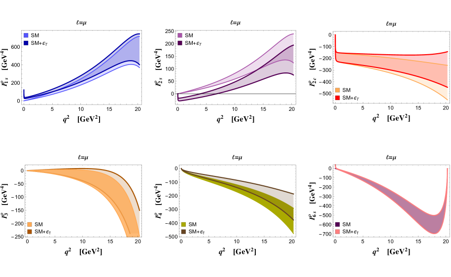
Figure 4: $\bar{B}\to\rho(\pi\pi)\,\mu^{-}\,\bar{\nu}_{\mu}$ mode: angular coefficient functions $I_{i}^{\rho}(q^{2})$ in set A, for SM and NP at the benchmark point. A zero in $I_{2s}^{\rho}(q^{2})$ appears in NP.

The other coefficient functions are drawn in Fig.5, and also in this case there is a zero in $I_{6c}^{\rho}(q^{2})$ which is absent in SM. The function $I_{7}^{\rho}$ vanishes in SM, and is only sensitive to the imaginary part of the NP couplings; it is shown in Fig.6. The angular functions for the $\tau$ modes are in Fig.7 and 8; $I_{7}^{\tau}$ vanishes since at the chosen benchmark point all the NP couplings $\epsilon^{\tau}$ are real. Also in this mode the coefficient $I_{6c}^{\rho}$ has a zero not appearing in SM.

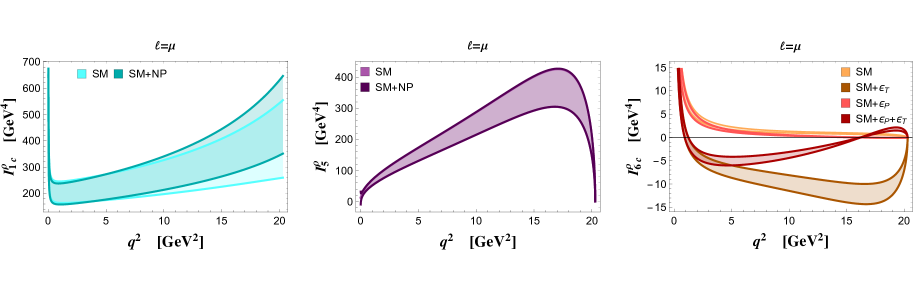
Figure 5: $\bar{B}\to\rho(\pi\pi)\,\mu^{-}\,\bar{\nu}_{\mu}$ mode: angular coefficient functions (set B) $I_{1c}^{\rho}(q^{2})$ (left), $I_{5}^{\rho}(q^{2})$ (middle) and $I_{6c}^{\rho}(q^{2})$ (right) for SM and NP at the benchmark point.

The measurement of the angular coefficients functions allows to determine the new couplings. Let us consider the ratios

$$R_{2s/1s}^{\rho}(q^{2}) = \displaystyle{\frac{I_{2s}^{\rho}(q^{2})}{I_{1s}^{\rho}(q^{2})}},$$ (11)

$$R_{2s/1s}^{a_{1},\,\parallel}(q^{2}) = \displaystyle{\frac{I_{2s,\parallel}^{a_{1}}(q^{2})}{I_{1s,\parallel}^{a_{1}}(q^{2})}},$$ (12)

and $R_{2s/1s}^{a_{1},\,\parallel}=R_{2c/1c}^{a_{1},\,\perp}$. In SM $R_{2s/1s}^{\rho}$ is form factor independent. In NP it is still form factor independent in the Large Energy limit, where $I_{2s}^{\rho}$ and $I_{1s}^{\rho}$ depend on $\xi_{\perp}^{\rho}$. As shown in Fig.9, the ratio (11) has a zero in the NP, not in SM, whose position $q_{0,\,\rho}^{2}$ has a weak form factor effect and depends only on $|\epsilon_{T}^{\mu}|$. In the Large Energy Limit we have

$$|\epsilon_{T}^{\mu}|^{2}=\frac{q_{0,\,\rho}^{2}}{16m_{B}^{2}}\frac{\lambda(m_{B}^{2},m_{\rho}^{2},q_{0,\,\rho}^{2})+2m_{B}^{2}m_{\rho}^{2}}{\lambda(m_{B}^{2},m_{\rho}^{2},q_{0,\,\rho}^{2})+2q_{0,\,\rho}^{2}m_{\rho}^{2}}.$$ (13)

Analogously, for the $(a_{1})_{\parallel}$ mode (and for $(a_{1})_{\perp}$ considering $R_{2c/1c}$) we have:

$$|\epsilon_{T}^{\mu}|^{2}=\frac{q_{0,\,a_{1}}^{2}}{16m_{B}^{2}}\frac{\lambda(m_{B}^{2},m_{a_{1}}^{2},q_{0,\,a_{1}}^{2})+2m_{B}^{2}m_{a_{1}}^{2}}{\lambda(m_{B}^{2},m_{a_{1}}^{2},q_{0,\,a_{1}}^{2})+2q_{0,\,a_{1}}^{2}m_{a_{1}}^{2}}\,\,.$$ (14)

The positions of the zeros in two modes are related, see Fig.10, and their independent measurement would provide a connection with the tensor operator.

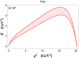
Figure 6: $\bar{B}\to\rho(\pi\pi)\,\mu^{-}\,\bar{\nu}_{\mu}$ mode: angular coefficient function $I_{7}^{\rho}(q^{2})$ in NP with the pseudoscalar operator at the benchmark point.

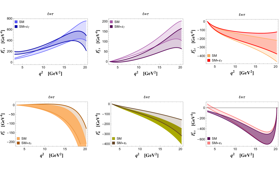
Figure 7: $\bar{B}\to\rho(\pi\pi)\,\tau^{-}\,\bar{\nu}_{\tau}$ mode: angular coefficient functions $I_{i}^{\rho}(q^{2})$ in set A for SM and NP at the benchmark point.

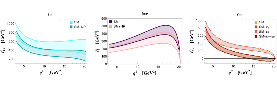
Figure 8: $\bar{B}\to\rho(\pi\pi)\,\tau^{-}\,\bar{\nu}_{\tau}$ mode: angular coefficient functions (set B) $I_{1c}^{\rho}(q^{2})$ (left), $I_{5}^{\rho}(q^{2})$ (middle) and $I_{6c}^{\rho}(q^{2})$ (right) for SM and NP at the benchmark point.

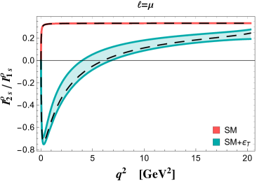
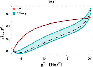
Figure 9: Ratio $\displaystyle R_{2s/1s}^{\rho}$ in (11) the modes $\bar{B}\to\rho(\pi\pi)\,\mu^{-}\,\bar{\nu}_{\mu}$ (left) and $\bar{B}\to\rho(\pi\pi)\,\tau^{-}\,\bar{\nu}_{\mu}$ (right), in SM and NP with tensor operator at the benchmark point. The dashed lines correspond to the Large Energy limit result (extrapolated to the full $q^{2}$ range).

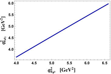
Figure 10: Relation between the position of the zeroes $q^{2}_{0}$ of the ratios (11) and (12) for the $B\to\rho$ and $B\to a_{1}$ modes, respectively.

Another suitable quantity is the angular coefficient function $I_{6c}^{\rho}$ shown in the right panel of Fig.5 in SM and NP, which is sensitive to $\epsilon_{V},\,\epsilon_{P},\,\epsilon_{T}$. At our benchmark point $\epsilon_{V}\simeq 0$, hence we keep only the $\epsilon_{P}$ and $\epsilon_{T}$ dependence:

$$\left(I_{6c}^{\rho}\right)|_{\epsilon_{V}\simeq 0}=(-2H_{t}^{\rho}) \Big{[}4H_{0}^{\rho}m_{\ell}^{2}-{\rm Re}[\epsilon_{T}]\,H_{L}^{NP,\,\rho}\,m_{\ell}\sqrt{q^{2}}+4{\rm Re}[\epsilon_{P}]\,H_{0}^{\rho}\frac{m_{\ell}}{m_{b}+m_{u}}q^{2}$$ (15)

$$-H_{L}^{NP,\rho}{\rm Re}[\epsilon_{P}\,\epsilon_{T}^{*}]\frac{(q^{2})^{3/2}}{m_{b}+m_{u}}\Big{]}\,\,.$$

Considering the $q^{2}$-dependence of the helicity amplitudes in Appendix B, we have the following possibilities:

• No NP, i.e. $\epsilon_{P}=\epsilon_{T}=0$. In this case, $I_{6c}^{\rho}=-8H_{t}^{\rho}H_{0}^{\rho}m_{\ell}^{2}$ does not have a zero, as shown in Fig.5 (right panel).

• NP with $\epsilon_{T}=0$ and $\epsilon_{P}\neq 0$. This gives:
  $(I_{6c}^{\rho})|_{\epsilon_{T}\simeq 0}=(-8H_{t}^{\rho}H_{0}^{\rho}\,m_{\ell})\left[m_{\ell}+{\rm Re}[\epsilon_{P}]\displaystyle{\frac{q^{2}}{m_{b}+m_{u}}}\right]$, with a zero at

  $$q^{2}_{0}=-\displaystyle{\frac{m_{b}+m_{u}}{m_{\ell}}\frac{1}{{\rm Re}[\epsilon_{P}]}}\,\,.$$ (16)

  This position is form factor independent, its measurement would result in a determination of ${\rm Re}[\epsilon_{P}]$. In the left panel of Fig.11 we show $I_{6c}^{\rho}$ enlarging the region where the zero is present for the benchmark ${\rm Re}[\epsilon_{P}]$, and in the middle panel we display $q^{2}_{0}$ versus ${\rm Re}[\epsilon_{P}]$ in the whole range for the coupling.

• NP with $\epsilon_{P}=0$ and $\epsilon_{T}\neq 0$, and
  $(I_{6c}^{\rho})|_{\epsilon_{P}\simeq 0}=(-2H_{t}^{\rho})\left[4H_{0}^{\rho}m_{\ell}^{2}-{\rm Re}[\epsilon_{T}]\,H_{L}^{NP,\,\rho}\,m_{\ell}\sqrt{q^{2}}\right]$. The zero is present if ${\rm Re}[\epsilon_{T}]>0$. The position has a form factor dependence, as shown in Fig.11 (right panel).

• NP with both $\epsilon_{P}\neq 0$ and $\epsilon_{T}\neq 0$. In this case both real and imaginary parts of $\epsilon_{P}$ and $\epsilon_{T}$ are involved. One can notice from Fig.5 that it is possible to have two zeros, nearly coinciding with those found in the previous two cases.

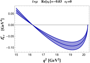
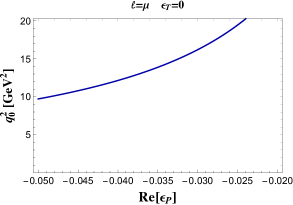
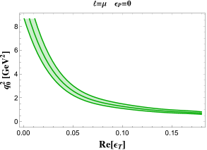
Figure 11: $\bar{B}\to\rho(\pi\pi)\,\mu^{-}\,\bar{\nu}_{\mu}$ mode: coefficient function $I_{6c}^{\rho}(q^{2})$ (left) and position $q_{0}^{2}$ varying ${\rm Re}(\epsilon_{P})$ with $\epsilon_{T}=0$ (middle panel), and ${\rm Re}(\epsilon_{T})$ with $\epsilon_{P}=0$ (right).

Integrating the 4d differential decay distribution several observables can be constructed.

• $q^{2}$-dependent forward-backward (FB) lepton asymmetry

  $$A_{FB}(q^{2})=\left[\int_{0}^{1}\,dcos\,\theta\,\displaystyle{\frac{d^{2}\Gamma}{dq^{2}dcos\,\theta}}-\int_{-1}^{0}\,dcos\,\theta\,\displaystyle{\frac{d^{2}\Gamma}{dq^{2}dcos\,\theta}}\right]\big{/}{\displaystyle{\frac{d\Gamma}{dq^{2}}}}\,\,\,,$$ (17)

  which is given in terms of the angular coefficient functions as

  $$A_{FB}(q^{2})=\frac{3(I_{6c}^{\rho}+2I_{6s}^{\rho})}{6I_{1c}^{\rho}+12I_{1s}^{\rho}-2I_{2c}^{\rho}-4I_{2s}^{\rho}}.$$ (18)

• Transverse forward-backward (TFB) asymmetry, the FB asymmetry for transversely polarized $\rho$, reading in terms of the angular coefficient functions as

  $$A_{FB}^{T}(q^{2})=\frac{3I_{6s}^{\rho}}{6I_{1s}^{\rho}-2I_{2s}^{\rho}}.$$ (19)

  For $\ell=\mu$ the asymmetries $A_{FB}$ and $A_{FB}^{T}$ are shown in Fig.12, for $\ell=\tau$ they are in Fig.14. In case of NP the zero of $A_{FB}$ in the $\tau$ mode is shifted. Moreover, $A_{FB}^{T}$ is very sensitive to the new operators, and in the case of $\tau$ it has a zero not present in SM. This is related to $I_{6s}^{\rho}$, with a zero in NP and not in SM.

• Observables sensitive to the $\rho$ polarization. We consider the differential branching ratio for longitudinally (L) and transversely (T) polarized $\rho$ as a function of $q^{2}$ or of one of the two angles $\theta$, $\theta_{V}$: ${d{\cal B}_{L(T)}}/{dq^{2}}$, ${d{\cal B}_{L(T)}}/{dcos\theta}$ and ${d{\cal B}_{L(T)}}/{dcos\theta_{V}}$. These observables are depicted for $\ell=\mu$ and for $\ell=\tau$ in Fig.13 and Fig.15, respectively.

Among all these quantities, the ones corresponding to transversely polarized $\rho$ depend only on $\epsilon_{T}$, as stressed in the legendae of the corresponding figures.

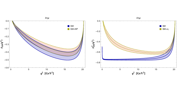
Figure 12: $\bar{B}\to\rho\,\mu^{-}\,\bar{\nu}_{\mu}$ mode: forward-backward lepton asymmetry (17) and (19) in SM and NP at the benchmark point.

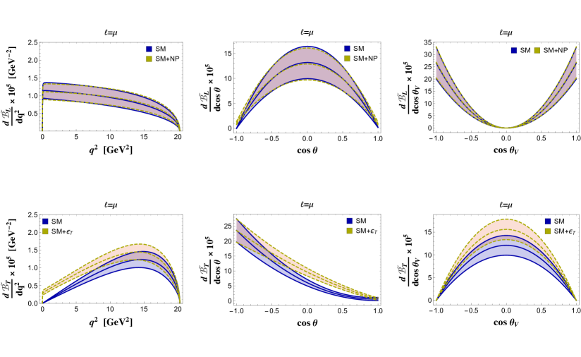
Figure 13: $\bar{B}\to\rho\,\mu^{-}\,\bar{\nu}_{\mu}$ mode: distributions ${d\tilde{\cal B}_{L}}/{dq^{2}}$, ${d\tilde{\cal B}_{L}}/{d\cos{\theta}}$ and ${d\tilde{\cal B}_{L}}/{d\cos{\theta_{V}}}$ (first line) and ${d\tilde{\cal B}_{T}}/{dq^{2}}$, ${d\tilde{\cal B}_{T}}/{d\cos{\theta}}$ and ${d\tilde{\cal B}_{T}}/{d\cos{\theta_{V}}}$ (second line), with $\tilde{\cal B}={\cal B}/{\cal B}(\rho\to\pi\pi)$, in SM and NP at the benchmark point.

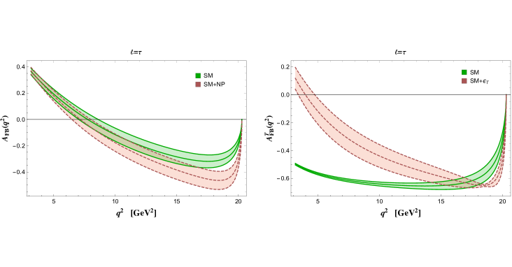
Figure 14: $\bar{B}\to\rho\,\tau^{-}\,\bar{\nu}_{\tau}$ mode: asymmetries (17) and (19) in SM and NP at the benchmark point.

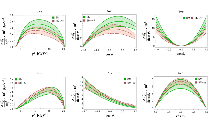
Figure 15: $\bar{B}\to\rho\,\tau^{-}\,\bar{\nu}_{\tau}$ mode: distributions ${d\tilde{\cal B}_{L}}/{dq^{2}}$, ${d\tilde{\cal B}_{L}}/{d\cos{\theta}}$ and ${d\tilde{\cal B}_{L}}/{d\cos{\theta_{V}}}$ (first line) and ${d\tilde{\cal B}_{T}}/{dq^{2}}$, ${d\tilde{\cal B}_{T}}/{d\cos{\theta}}$ and ${d\tilde{\cal B}_{T}}/{d\cos{\theta_{V}}}$ (second line), with $\tilde{\cal B}={\cal B}/{\cal B}(\rho\to\pi\pi)$, in SM and NP at the benchmark point.

Integrating the distributions, we obtain in SM the longitudinal and transverse polarization fractions and the branching fractions:

$$F_{L}(\bar{B}\to\rho\mu^{-}\bar{\nu}_{\mu})|_{SM} = 0.52\pm 0.15$$

$$F_{T}(\bar{B}\to\rho\mu^{-}\bar{\nu}_{\mu})|_{SM} = 0.48\pm 0.11$$

$${\cal B}({\bar{B}}^{0}\to\rho^{+}\mu^{-}\bar{\nu}_{\mu})|_{SM} = (3.37\pm 0.52)\times 10^{-4}\times\left(\frac{|V_{ub}|}{0.0035}\right)^{2},$$ (20)

$$F_{L}(\bar{B}\to\rho\tau^{-}\bar{\nu}_{\tau})|_{SM} = 0.50\pm 0.13$$

$$F_{T}(\bar{B}\to\rho\tau^{-}\bar{\nu}_{\tau})|_{SM} = 0.50\pm 0.12$$

$${\cal B}({\bar{B}}^{0}\to\rho^{+}\tau^{-}\bar{\nu}_{\tau})|_{SM} = (1.80\pm 0.25)\times 10^{-4}\times\left(\frac{|V_{ub}|}{0.0035}\right)^{2}.$$ (21)

For the $B\to\pi$ mode we have:

$${\cal B}({\bar{B}}^{0}\to\pi^{+}\mu^{-}\bar{\nu}_{\mu})|_{SM} = (1.5\pm 0.1)\times 10^{-4}\times\left(\frac{|V_{ub}|}{0.0035}\right)^{2}$$

$${\cal B}({\bar{B}}^{0}\to\pi^{+}\tau^{-}\bar{\nu}_{\tau})|_{SM} = (0.92\pm 0.06)\times 10^{-4}\times\left(\frac{|V_{ub}|}{0.0035}\right)^{2}.$$ (22)

The ratios

$$R_{\pi}=\frac{{\cal B}({\bar{B}}\to\pi\tau^{-}{\bar{\nu}}_{\tau})}{{\cal B}({\bar{B}}\to\pi\ell^{-}{\bar{\nu}}_{\ell})}\,\,\,,\hskip 28.45274ptR_{\rho}=\frac{{\cal B}({\bar{B}}\to\rho\tau^{-}{\bar{\nu}}_{\tau})}{{\cal B}({\bar{B}}\to\rho\ell^{-}{\bar{\nu}}_{\ell})}\,$$ (23)

are modified by the New Physics operators in (1). The results in SM and NP are collected in Table 1, with the errors obtained considering the uncertainties in the hadronic form factors. The deviations are correlated when the new operators are included in the effective Hamiltonian and, as shown in Fig.16, large effects are possible in corners of the parameter space of the new effective couplings.

	SM	NP (benchmark point)
$R_{\pi}$	$0.60\pm 0.01$	$0.75\pm 0.02$
$R_{\rho}$	$0.53\pm 0.02$	$0.49\pm 0.02$

Table 1: Ratios $R_{\pi}$ and $R_{\rho}$ in Eq.(23) in SM and in NP at the benchmark point.

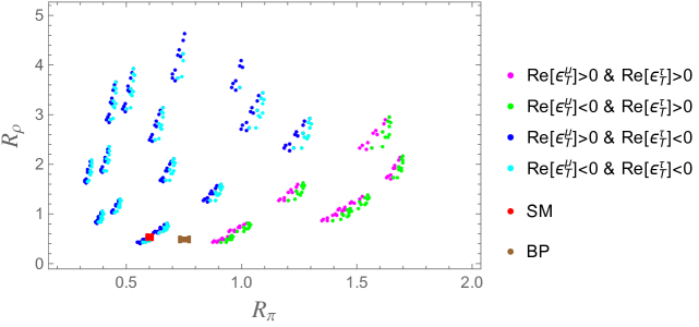
Figure 16: Correlation between $R_{\rho}$ and $R_{\pi}$ in Eq.(23) with only the tensor operator added to the SM effective Hamiltonian. The colors correspond to the different signs of ${\rm Re}(\epsilon_{T}^{\mu})$ and ${\rm Re}(\epsilon_{T}^{\tau})$ in the full range of the parameter space. The red and brown points are the SM and NP result at the benchmark point, respectively.

Concerning $R_{\pi}$ in SM, the value $R_{\pi}=0.641(17)$ is obtained using lattice form factors at large $q^{2}$ [67], the range $[0.654,0.764]$ is found in [68], $R_{\pi}=0.7$ together with $R_{\rho}\simeq 0.573$ is found using form factors computed in pQCD [69], $R_{\pi}\simeq 0.731$ and $R_{\rho}\simeq 0.585$ are quoted in [70]. The effect of a new charged Higgs reduces the SM result for $R_{\pi}$ and $R_{\rho}$ [71]. Considering a single NP operator per time, values for $R_{\pi}$ up to $\simeq 4$ are obtained in [68], the range $[0.5,\,1.38]$ is found in [69], while the inclusion only of the pseudoscalar and scalar operators in the effective Hamiltonian gives $R_{\pi}\in[0.5,\,1.2]$ [49].

5 Remarks about the mode $\bar{B}\to a_{1}(1260)\ell^{-}\bar{\nu}_{\ell}$

As for $\bar{B}\to\rho(\pi\pi)\ell^{-}\bar{\nu}_{\ell}$, the channel $\bar{B}\to a_{1}(\rho\pi)\ell^{-}\bar{\nu}_{\ell}$ can be numerically analyzed in SM and in the NP extension Eq.(1) using the same benchmark points for the couplings $\epsilon^{\ell}_{V,S,T}$, and the expressions for the angular coefficient functions in terms of the form factors. Exclusive hadronic $B$ decays into $a_{1}(1260)$ have been analyzed at the $B$ factories considering the dominant $a_{1}\to\rho\pi$ mode. In particular, $B^{0}\to a_{1}(1260)^{\pm}\pi^{\mp}$ have been scrutinized by BABAR and Belle Collaborations to carry out measurements of CP violation [72, 73, 74].

Observation and measurements of the semileptonic $\bar{B}\to a_{1}$ mode are within the present experimental reach, in particular at Belle II. The theoretical study of $\bar{B}\to a_{1}\ell^{-}\bar{\nu}_{\ell}$ requires an assessment of the accuracy of the hadronic quantities. The $\bar{B}\to a_{1}$ form factors have been evaluated by different methods [75, 76, 77, 78, 79, 80, 81, 82, 83, 84], but a comparative evaluation of the uncertainties has not be done so far. To present numerical examples, we use the set of form factors in Ref.[82], for which the uncertainty of about $20\%$ is quoted. The angular coefficient functions, for the $\mu$ and $\tau$ modes and for both the $\rho$ polarizations, are depicted in Figs.17, 18, 19 and 20. In general, the hadronic uncertainties obscure the effects of the NP operators, confirming the necessity of more precise determinations. Nevertheless, there are coefficient functions in which deviations from SM can be observed, namely $I^{a_{1}}_{2s,\parallel}(q^{2})$, $I^{a_{1}}_{6c,\parallel}(q^{2})$ (Fig.17) and $I^{a_{1}}_{2c,\perp}(q^{2})$ (Fig. 19) for the $\mu$ channel, $I^{a_{1}}_{1s,\parallel}(q^{2})$, $I^{a_{1}}_{6s,\parallel}(q^{2})$ (Fig.18) and $I^{a_{1}}_{1c\perp}(q^{2})$, $I^{a_{1}}_{6c\perp}(q^{2})$ (Fig.20) for the $\tau$ mode. On the other hand, the forward/backward lepton asymmetry shows sizeable deviations from SM in the case of $\tau$, as shown in Fig.21.

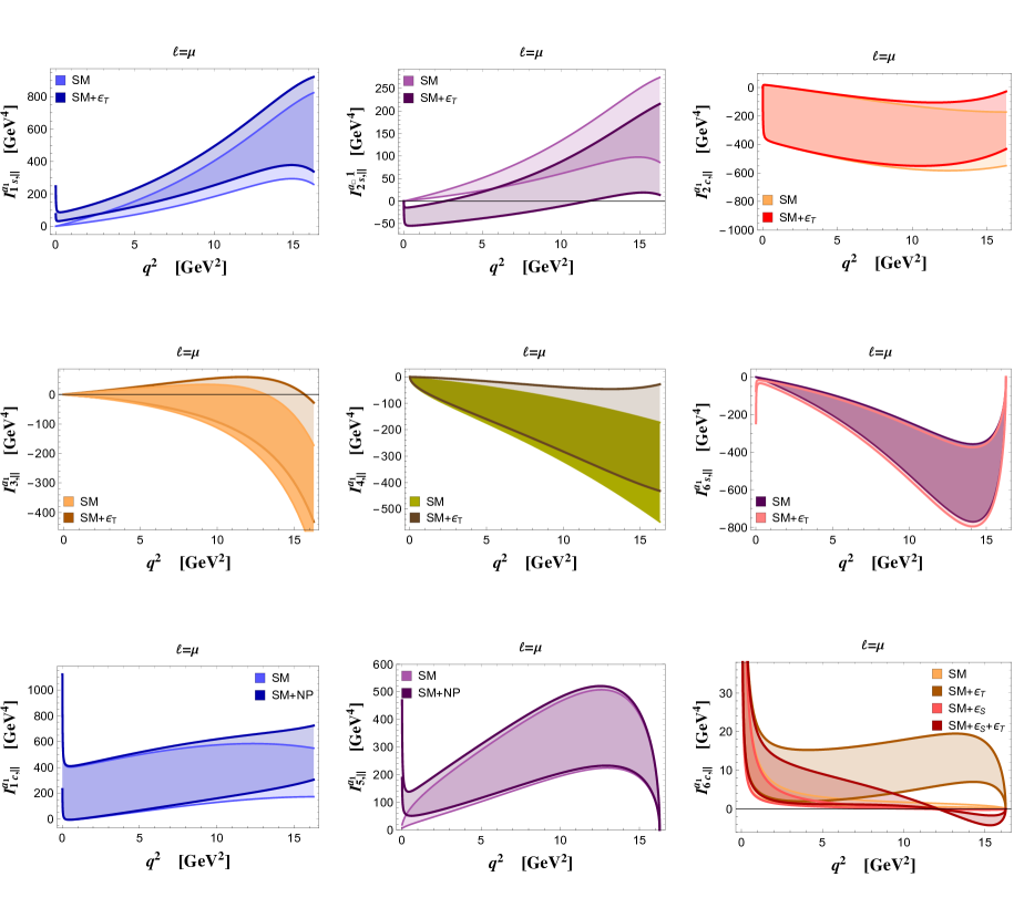
Figure 17: $\bar{B}\to a_{1}(\rho_{\parallel}\pi)\,\mu^{-}\,\bar{\nu}_{\mu}$ mode: angular coefficient functions in (3) for SM and NP at the benchmark point, using the form factors in [82]. The band widths are due to the uncertainty in the set of form factors.

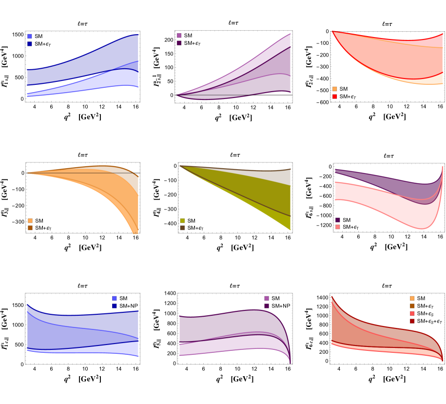
Figure 18: $\bar{B}\to a_{1}(\rho_{\parallel}\pi)\,\tau^{-}\,\bar{\nu}_{\tau}$ mode, angular coefficient functions with same notations as in Fig.17.

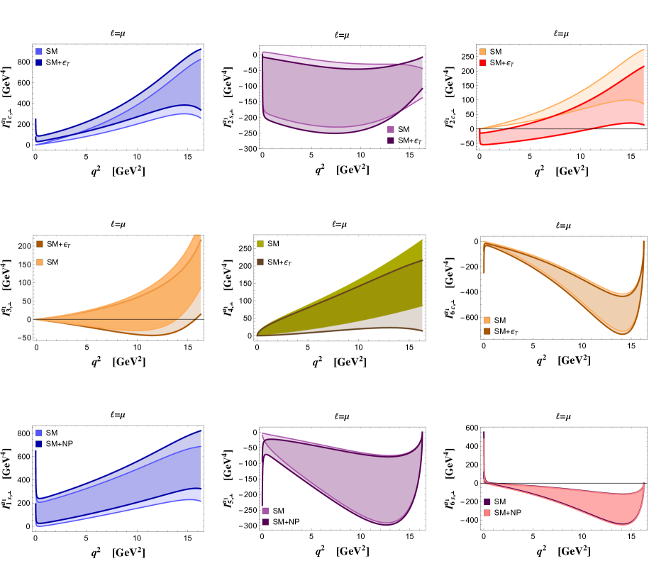
Figure 19: $\bar{B}\to a_{1}(\rho_{\perp}\pi)\,\mu^{-}\,\bar{\nu}_{\mu}$ mode, angular coefficient functions with same notations as in Fig.17.

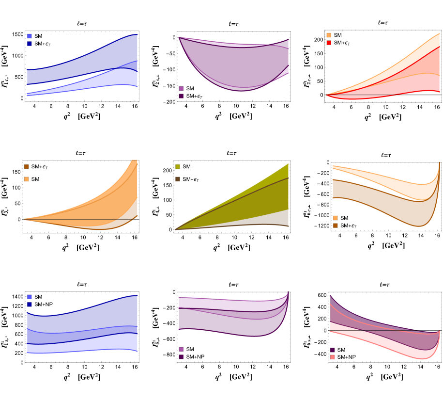
Figure 20: $\bar{B}\to a_{1}(\rho_{\perp}\pi)\,\tau^{-}\,\bar{\nu}_{\tau}$ mode, angular coefficient functions with same notations as in Fig.17.

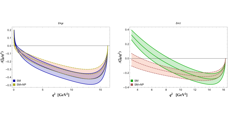
Figure 21: $\bar{B}\to a_{1}\,\ell^{-}\,\bar{\nu}_{\ell}$ mode: FB lepton asymmetries for $\ell=\mu$ (left) and $\tau$ (right).

In the ratio $\displaystyle R_{a_{1}}=\frac{{\cal B}({\bar{B}}\to a_{1}\tau^{-}{\bar{\nu}}_{\tau})}{{\cal B}({\bar{B}}\to a_{1}\ell^{-}{\bar{\nu}}_{\ell})}$ the form factor uncertainty is mild. We obtain, in the SM and for NP at the benchmark point,

$$R_{a_{1}}^{SM}=0.44\pm 0.07\,\,\,,\hskip 28.45274ptR_{a_{1}}^{NP}=0.67\pm 0.12\,\,\,.$$ (24)

The individual branching fractions in SM, in this model of form factors, are ${\cal B}(\bar{B}\to a_{1}^{-}\,\mu^{-}\bar{\nu}_{\mu})=(3.0\pm 1.7)\times 10^{-4}$ and ${\cal B}(\bar{B}\to a_{1}^{-}\,\tau^{-}\bar{\nu}_{\tau})=(1.3\pm 0.6)\times 10^{-4}$ [82].

We can now summarize the synergies between the various considered modes to provide possible evidences of NP in semileptonic $b\to u$ transitions.

• The presence of the tensor structure in the effective Hamiltonian can be established independently of the presence of the other operators, looking at deviations of the observables that depend only on $\epsilon_{T}$. These are the observables involving transversely polarized $\rho$ and $a_{1}$. Moreover, it is possible to tightly constrain $|\epsilon_{T}|$ looking at the zero of the ratios defined in Eqs.(11), (12). A correlation between the position of the zero in the $\rho$ and $a_{1}$ modes should be observed, as in Fig.10.

• If a pseudoscalar operator is present, without other NP structures, deviations should be observed in leptonic $B$ decays and in the semileptonic decay to $\rho$, not in semileptonic decays to $\pi$ and $a_{1}$. Determining the position of the zero in $I_{6c}^{\rho}$ allows to constrain ${\rm Re}[\epsilon_{P}]$. Zeroes should not be present in $I_{6c,\parallel}^{a_{1}}$.

• If a scalar operator is present, without additional NP structures, deviations should be observed in semileptonic $B$ decays to $\pi$ and $a_{1}$. In particular, a zero would be present in $I_{6c,\parallel}^{a_{1}}$, not in $I_{6c}^{\rho}$.

• The simultaneous presence of all the operators would manifest in a more involved pattern of deviations. However, such deviations are correlated in the two modes, and the pattern of correlation can be used to assess the role of the various new terms in (1).

• Precise measurements of modes with final $\tau$ provide new important tests of LFU. The determination of $R_{\rho}$ and $R_{\pi}$ would give information on the relative sign of ${\rm Re}[\epsilon_{T}^{\mu}]$ and ${\rm Re}[\epsilon_{T}^{\tau}]$, as shown in Fig.16. In the $a_{1}$ channel deviations are also expected. However, in this case the reconstruction of the modes with $\tau$ is challenging: for example, using the 3 prong channel for the $\tau$ reconstruction implies to consider a final state comprising six light mesons.

6 Conclusions and perspectives

The questions arised by the anomalies in $b\to c$ semileptonic modes call for new analyses on the CKM suppressed semileptonic $b\to u$ modes, for which precise measurements are expected. We have considered an enlarged SM effective Hamiltonian including additional D=6 operators, and looked for the impact of the new terms on $\bar{B}\to\rho(\pi\pi)\ell^{-}\bar{\nu}_{\ell}$ and $\bar{B}\to a_{1}(\rho\pi)\ell^{-}\bar{\nu}_{\ell}$. We have constructed the 4d differential distribution for both the modes, finding that they are sensitive to different NP operators. The different quantum numbers of light mesons in the two processes act a selection on the contributions of the NP terms, therefore the two modes provide complementary information about the role of the new operators in Eq.(1). This motivates their consideration. We have constrained the parameter space of the effective coupling constants from current data on purely leptonic and semileptonic $B$ modes into a pseudoscalar meson, and considered the impact on $\bar{B}\to\rho\ell^{-}\bar{\nu}_{\ell}$. Among the various observables, we have found that a few angular coefficients present zeroes that do not appear in SM, the observation of which whould represent a support towards the confirmation of NP effects. We have defined integrated decay distributions, useful for comparing the modes into $\mu$ and $\tau$, with the aim of further testing LF universality. In the perspective of precision analyses, the theoretical error connected to the hadronic matrix elements represents a sizable uncertainty needing to be reduced, in particular for the $a_{1}$ mode. The combination of different determinations based on QCD (QCD sum rules and lattice QCD), obtained in their respective domain of validity, can be a strategy for reducing the theoretical uncertainty. The Large Energy limit, in which the number of hadronic form factors is reduced, also represents a way to analyze these two modes. The possibility of finding deviations from SM fully justifies the careful scrutiny of such promising processes.

Acknowledgements. This study has been carried out within the INFN project (Iniziativa Specifica) QFT-HEP.

Appendix A Hadronic matrix elements

For $M_{u}=\pi^{+}$ meson, the weak matrix elements are written in terms of form factors as follows:

$$\langle\pi(p^{\prime})|{\bar{u}}\gamma_{\mu}b|{\bar{B}}(p)\rangle = f_{+}^{B\to\pi}(q^{2})\Big{[}p_{\mu}+p_{\mu}^{\prime}-\frac{m_{B}^{2}-m_{\pi}^{2}}{q^{2}}q_{\mu}\Big{]}+f_{0}^{B\to\pi}(q^{2})\frac{m_{B}^{2}-m_{\pi}^{2}}{q^{2}}q_{\mu}$$

$$\langle\pi(p^{\prime})|{\bar{u}}b|{\bar{B}}(p)\rangle = f_{S}^{B\to\pi}(q^{2})$$

$$\langle\pi(p^{\prime})|{\bar{u}}\sigma_{\mu\nu}b|{\bar{B}}(p)\rangle = -i\frac{2f_{T}^{B\to\pi}(q^{2})}{m_{B}+m_{\pi}}\big{[}p_{\mu}p_{\nu}^{\prime}-p_{\nu}p^{\prime}_{\mu}\big{]}$$ (A.1)

$$\langle\pi(p^{\prime})|{\bar{u}}\sigma_{\mu\nu}\gamma_{5}b|{\bar{B}}(p)\rangle = -\frac{2f_{T}^{B\to\pi}(q^{2})}{m_{B}+m_{\pi}}\epsilon_{\mu\nu\alpha\beta}\,p^{\alpha}p^{\prime\beta}\,\,\,,$$

where $\epsilon^{0123}=+1$. The relation $f_{S}^{B\to\pi}(q^{2})=\displaystyle\frac{m_{B}^{2}-m_{\pi}^{2}}{m_{b}-m_{u}}f_{0}^{B\to\pi}(q^{2})$ holds.

For $M_{u}=\rho^{+}$ the various matrix elements, expressed in terms of form factors (with $\epsilon$ the $\rho$ polarization vector), read:

$$\langle\rho(p^{\prime},\epsilon)|{\bar{u}}\gamma_{\mu}(1-\gamma_{5})b|{\bar{B}}(p)\rangle = -{2V^{B\to\rho}(q^{2})\over m_{B}+m_{\rho}}i\epsilon_{\mu\nu\alpha\beta}\epsilon^{*\nu}p^{\alpha}p^{\prime\beta}$$ (A.2)

$$- \Big{\{}(m_{B}+m_{\rho})\left[\epsilon^{*}_{\mu}-{(\epsilon^{*}\cdot q)\over q^{2}}q_{\mu}\right]A_{1}^{B\to\rho}(q^{2})$$

$$- {(\epsilon^{*}\cdot q)\over m_{B}+m_{\rho}}\left[(p+p^{\prime})_{\mu}-{m_{B}^{2}-m_{\rho}^{2}\over q^{2}}q_{\mu}\right]A_{2}^{B\to\rho}(q^{2})$$

$$+ (\epsilon^{*}\cdot q){2m_{\rho}\over q^{2}}q_{\mu}A_{0}^{B\to\rho}(q^{2})\Big{\}}\,\,\,,$$

with the condition $\displaystyle A_{0}^{B\to\rho}(0)=\frac{m_{B}+m_{\rho}}{2m_{\rho}}A_{1}^{B\to\rho}(0)-\frac{m_{B}-m_{\rho}}{2m_{\rho}}A_{2}^{B\to\rho}(0)$, and

$$\langle\rho(p^{\prime},\epsilon)|{\bar{u}}\gamma_{5}b|{\bar{B}}(p)\rangle = -\frac{2m_{\rho}}{m_{b}+m_{u}}(\epsilon^{*}\cdot q)A_{0}^{B\to\rho}(q^{2})$$ (A.3)

$$\langle\rho(p^{\prime},\epsilon)|{\bar{u}}\sigma_{\mu\nu}b|{\bar{B}}(p)\rangle = T_{0}^{B\to\rho}(q^{2}){\epsilon^{*}\cdot q\over(m_{B}+m_{\rho})^{2}}\epsilon_{\mu\nu\alpha\beta}p^{\alpha}p^{\prime\beta}$$ (A.4)

$$+ T_{1}^{B\to\rho}(q^{2})\epsilon_{\mu\nu\alpha\beta}p^{\alpha}\epsilon^{*\beta}+T_{2}^{B\to\rho}(q^{2})\epsilon_{\mu\nu\alpha\beta}p^{\prime\alpha}\epsilon^{*\beta}$$

$$\langle\rho(p^{\prime},\epsilon)|{\bar{u}}\sigma_{\mu\nu}\gamma_{5}b|{\bar{B}}(p)\rangle = i\,T_{0}^{B\to\rho}(q^{2}){\epsilon^{*}\cdot q\over(m_{B}+m_{\rho})^{2}}(p_{\mu}p^{\prime}_{\nu}-p_{\nu}p^{\prime}_{\mu})$$ (A.5)

$$+i\,T_{1}^{B\to\rho}(q^{2})(p_{\mu}\epsilon_{\nu}^{*}-\epsilon_{\mu}^{*}p_{\nu})+i\,T_{2}^{B\to\rho}(q^{2})(p^{\prime}_{\mu}\epsilon_{\nu}^{*}-\epsilon_{\mu}^{*}p^{\prime}_{\nu})\,\,.\,\,\,$$

For $M_{u}=a_{1}^{+}$ we use the decomposition:

$$\langle a_{1}(p^{\prime},\epsilon)|{\bar{u}}\gamma_{\mu}(1-\gamma_{5})b|{\bar{B}}(p)\rangle = {2A^{B\to a_{1}}(q^{2})\over m_{B}+m_{a_{1}}}i\epsilon_{\mu\nu\alpha\beta}\epsilon^{*\nu}p^{\alpha}p^{\prime\beta}$$ (A.6)

$$+ \Big{\{}(m_{B}+m_{a_{1}})\left[\epsilon^{*}_{\mu}-{(\epsilon^{*}\cdot q)\over q^{2}}q_{\mu}\right]V_{1}^{B\to a_{1}}(q^{2})$$

$$- {(\epsilon^{*}\cdot q)\over m_{B}+m_{a_{1}}}\left[(p+p^{\prime})_{\mu}-{m_{B}^{2}-m_{a_{1}}^{2}\over q^{2}}q_{\mu}\right]V_{2}^{B\to a_{1}}(q^{2})$$

$$+ (\epsilon^{*}\cdot q){2m_{a_{1}}\over q^{2}}q_{\mu}V_{0}^{B\to a_{1}}(q^{2})\Big{\}}$$

with the condition $\displaystyle V_{0}^{B\to a_{1}}(0)=\frac{m_{B}+m_{a_{1}}}{2m_{a_{1}}}V_{1}^{B\to a_{1}}(0)-\frac{m_{B}-m_{a_{1}}}{2m_{a_{1}}}V_{2}^{B\to a_{1}}(0)$, and

$$\langle a_{1}(p^{\prime},\epsilon)|{\bar{u}}b|{\bar{B}}(p)\rangle = \frac{2m_{a_{1}}}{m_{b}-m_{u}}(\epsilon^{*}\cdot q)V_{0}^{B\to a_{1}}(q^{2})$$ (A.7)

$$\langle a_{1}(p^{\prime},\epsilon)|{\bar{u}}\sigma_{\mu\nu}b|{\bar{B}}(p)\rangle = i\,T_{0}^{B\to a_{1}}(q^{2}){\epsilon^{*}\cdot q\over(m_{B}+m_{a_{1}})^{2}}(p_{\mu}p^{\prime}_{\nu}-p_{\nu}p^{\prime}_{\mu})$$ (A.8)

$$+i\,T_{1}^{B\to a_{1}}(q^{2})(p_{\mu}\epsilon_{\nu}^{*}-\epsilon_{\mu}^{*}p_{\nu})+i\,T_{2}^{B\to a_{1}}(q^{2})(p^{\prime}_{\mu}\epsilon_{\nu}^{*}-\epsilon_{\mu}^{*}p^{\prime}_{\nu})\,\,\,\,\,\,\,$$

$$\langle a_{1}(p^{\prime},\epsilon)|{\bar{u}}\sigma_{\mu\nu}\gamma_{5}b|{\bar{B}}(p)\rangle = T_{0}^{B\to a_{1}}(q^{2}){\epsilon^{*}\cdot q\over(m_{B}+m_{a_{1}})^{2}}\epsilon_{\mu\nu\alpha\beta}p^{\alpha}p^{\prime\beta}$$ (A.9)

$$+ T_{1}^{B\to a_{1}}(q^{2})\epsilon_{\mu\nu\alpha\beta}p^{\alpha}\epsilon^{*\beta}+T_{2}^{B\to a_{1}}(q^{2})\epsilon_{\mu\nu\alpha\beta}p^{\prime\alpha}\epsilon^{*\beta}$$

In the large energy (large recoil) limit for the light meson the weak matrix elements can be expressed in terms of a smaller number of form factors. We define $E=\displaystyle\frac{m_{B}^{2}+m^{2}-q^{2}}{2m_{B}}$ the light meson energy in the $B$ rest-frame, and $m$ the light meson mass. The $B$ four-velocity is defined from $p=m_{B}v$, and $n_{-}$ is a light-like four-vector along $p^{\prime}$: $p^{\prime}=E\,n_{-}$. In the large recoil configuration, for $\displaystyle E\simeq\frac{m_{B}}{2}$, the light quark u carries almost all the momentum of the light meson: $p^{\prime}_{u\,\mu}=E\,(n_{-})_{\mu}+k_{\mu}$, with the residual momentum $k\ll E$. Using, e.g., a eikonal formulation of the weak current, this allows to express the form factors in terms of universal functions $\xi_{i}(E)$ [50, 51]. For $B\to\pi$, a single form factor $\xi_{\pi}(E)$ parametrizes the matrix elements,

$$\langle\pi(p^{\prime})|{\bar{u}}\gamma_{\mu}b|{\bar{B}}(p)\rangle = 2E\,\xi_{\pi}(E)(n_{-})_{\mu}$$

$$\langle\pi(p^{\prime})|{\bar{u}}\sigma_{\mu\nu}q^{\nu}b|{\bar{B}}(p)\rangle = 2iE\,\xi_{\pi}(E)\Big{[}(m_{B}-E)(n_{-})_{\mu}-m_{B}v_{\mu}\Big{]}\,\,\,.$$ (A.10)

For $B\to\rho$ there are two independent form factors, $\xi_{\perp}^{\rho}(E)$ and $\xi_{\parallel}^{\rho}(E)$,

$$\langle\rho(p^{\prime},\epsilon)|{\bar{u}}\gamma_{\mu}b|{\bar{B}}(p)\rangle = 2i\,E\xi_{\perp}^{\rho}(E)\epsilon_{\mu\nu\alpha\beta}\epsilon^{*\nu}(n_{-})^{\alpha}v^{\beta}$$

$$\langle\rho(p^{\prime},\epsilon)|{\bar{u}}\gamma_{\mu}\gamma_{5}b|{\bar{B}}(p)\rangle = 2E\Big{\{}\xi_{\perp}^{\rho}(E)\big{[}\epsilon^{*}_{\mu}-(\epsilon^{*}\cdot v)(n_{-})_{\mu}\big{]}+\xi_{\parallel}^{\rho}(E)(\epsilon^{*}\cdot v)(n_{-})_{\mu}\Big{\}}$$

$$\langle\rho(p^{\prime},\epsilon)|{\bar{u}}\sigma_{\mu\nu}q^{\nu}b|{\bar{B}}(p)\rangle = 2Em_{B}\xi_{\perp}^{\rho}(E)\epsilon_{\mu\nu\alpha\beta}\epsilon^{*\nu}v^{\alpha}(n_{-})^{\beta}$$ (A.11)

$$\langle\rho(p^{\prime},\epsilon)|{\bar{u}}\sigma_{\mu\nu}\gamma_{5}q^{\nu}b|{\bar{B}}(p)\rangle = -2iE\,\Big{\{}\xi_{\perp}^{\rho}(E)m_{B}\big{[}\epsilon^{*}_{\mu}-(\epsilon^{*}\cdot v)(n_{-})_{\mu}\big{]}$$

$$\hskip 28.45274pt+\xi_{\parallel}^{\rho}(E)(\epsilon^{*}\cdot v)\Big{[}(m_{B}-E)(n_{-})_{\mu}-m_{B}v_{\mu}\Big{]}\Big{\}},$$

and two independent $\xi_{\perp}^{a_{1}}(E)$ and $\xi_{\parallel}^{a_{1}}(E)$ for factors are also involved for $a_{1}$,

$$\langle a_{1}(p^{\prime},\epsilon)|{\bar{u}}\gamma_{\mu}\gamma_{5}b|{\bar{B}}(p)\rangle = -2i\,E\,\xi_{\perp}^{a_{1}}(E)\epsilon_{\mu\nu\alpha\beta}\epsilon^{*\nu}(n_{-})^{\alpha}v^{\beta}$$

$$\langle a_{1}(p^{\prime},\epsilon)|{\bar{u}}\gamma_{\mu}b|{\bar{B}}(p)\rangle = -2E\,\Big{\{}\xi_{\perp}^{a_{1}}(E)\big{[}\epsilon^{*}_{\mu}-(\epsilon^{*}\cdot v)(n_{-})_{\mu}\big{]}+\xi_{\parallel}^{a_{1}}(E)(\epsilon^{*}\cdot v)(n_{-})_{\mu}\Big{\}}\hskip 28.45274pt$$

$$\langle a_{1}(p^{\prime},\epsilon)|{\bar{u}}\sigma_{\mu\nu}q^{\nu}\gamma_{5}b|{\bar{B}}(p)\rangle = 2Em_{B}\xi_{\perp}^{a_{1}}(E)\epsilon_{\mu\nu\alpha\beta}\epsilon^{*\nu}v^{\alpha}(n_{-})^{\beta}$$ (A.12)

$$\langle a_{1}(p^{\prime},\epsilon)|{\bar{u}}\sigma_{\mu\nu}q^{\nu}b|{\bar{B}}(p)\rangle = -2iE\Big{\{}\xi_{\perp}^{a_{1}}(E)m_{B}\big{[}\epsilon^{*}_{\mu}-(\epsilon^{*}\cdot v)(n_{-})_{\mu}\big{]}$$

$$\hskip 28.45274pt+\xi_{\parallel}^{a_{1}}(E)(\epsilon^{*}\cdot v)\Big{[}(m_{B}-E)(n_{-})_{\mu}-m_{B}v_{\mu}\Big{]}\Big{\}}\,\,.$$

Comparing Eqs.(A.1)-(A.8) with (A.10)-(A.12), the relations among the form factors and their large energy limit expressions can be worked out. For $B\to\pi$ they are:

$$f_{+}^{B\to\pi}(q^{2})=\frac{m_{B}}{2E}f_{0}^{B\to\pi}(q^{2})=\frac{m_{B}}{m_{B}+m_{\pi}}f_{T}^{B\to\pi}(q^{2})=\xi_{\pi}(E)\,\,,$$ (A.13)

for $B\to\rho$:

$$\frac{m_{B}}{m_{B}+m_{\rho}}V^{B\to\rho}(q^{2}) = \frac{m_{B}+m_{\rho}}{2E}A_{1}^{B\to\rho}(q^{2})=\xi_{\perp}^{\rho}(E)$$

$$\frac{m_{\rho}}{E}A_{0}^{B\to\rho}(q^{2}) = \frac{m_{B}+m_{\rho}}{2E}A_{1}^{B\to\rho}(q^{2})-\frac{m_{B}-m_{\rho}}{m_{B}}A_{2}^{B\to\rho}(q^{2})=\xi_{\parallel}^{\rho}(E)\hskip 28.45274pt$$

$$T_{1}^{B\to\rho}(q^{2}) = 0$$ (A.14)

$$T_{2}^{B\to\rho}(q^{2}) = 2\xi_{\perp}^{\rho}(E)$$

$$T_{0}^{B\to\rho}(q^{2}) = 2\xi_{\parallel}^{\rho}(E)\,\,,$$

and for $B\to a_{1}$:

$$\frac{m_{B}}{m_{B}+m_{a_{1}}}A^{B\to a_{1}}(q^{2}) = \frac{m_{B}+m_{a_{1}}}{2E}V_{1}^{B\to a_{1}}(q^{2})=\xi_{\perp}^{a_{1}}(E)$$

$$\frac{m_{a_{1}}}{E}V_{0}^{B\to a_{1}}(q^{2}) = \frac{m_{B}+m_{a_{1}}}{2E}V_{1}^{B\to a_{1}}(q^{2})-\frac{m_{B}-m_{a_{1}}}{m_{B}}V_{2}^{B\to a_{1}}(q^{2})=\xi_{\parallel}^{a_{1}}(E)\hskip 28.45274pt$$

$$T_{1}^{B\to{a_{1}}}(q^{2}) = 0$$ (A.15)

$$T_{2}^{B\to{a_{1}}}(q^{2}) = 2\xi^{a_{1}}_{\perp}(E)$$

$$T_{0}^{B\to{a_{1}}}(q^{2}) = 2\xi_{\parallel}^{a_{1}}(E)\,\,.$$

The functions $\xi_{\pi}$, $\xi_{\parallel}^{\rho}$ and $\xi_{\perp}^{\rho}$ have been determined by light-cone QCD sum rules within the Soft Collinear Effective Theory, using $B$ meson light-cone distribution amplitudes [85, 86, 87].

Appendix B Angular coefficient functions

Here we collect the expressions of the angular coefficient functions in Eqs.(3,3). The general form of the ${\bar{B}}\to V\ell^{-}{\bar{\nu}}_{\ell}$ decay amplitude, with $V=\rho$ and $a_{1}$,

$${\cal A}({\bar{B}}\to V\ell^{-}{\bar{\nu}}_{\ell})={G_{F}\over\sqrt{2}}V_{ub} \big{[}(1+\epsilon_{V}^{\ell})H^{SM}_{\mu}L^{SM\,\mu}$$ (B.1)

$$+\epsilon_{S}^{\ell}H^{NP,S}L^{NP,S}+\epsilon_{P}^{\ell}H^{NP,P}L^{NP,P}+\epsilon_{T}^{\ell}H^{NP,T}_{\mu\nu}L^{NP,T\,\mu\nu}\big{]},\hskip 28.45274pt$$

is given in terms of the quark current matrix elements

$$H^{SM}_{\mu}(m) = \langle V(p_{V},\epsilon(m))|{\bar{u}}\gamma_{\mu}(1-\gamma_{5})b|{\bar{B}}(p_{B})\rangle=\epsilon^{*\alpha}(m)T_{\mu\alpha}$$ (B.2)

$$H^{NP,S}(m) = \langle V(p_{V},\epsilon(m))|{\bar{u}}b|{\bar{B}}(p_{B})\rangle=\epsilon^{*\alpha}(m)T^{NP,S}_{\alpha}$$ (B.3)

$$H^{NP,P}_{\mu}(m) = \langle V(p_{V},\epsilon(m))|{\bar{u}}\gamma_{5}b|{\bar{B}}(p_{B})\rangle=\epsilon^{*\alpha}(m)T^{NP,P}_{\alpha}$$ (B.4)

$$H^{NP,T}_{\mu\nu}(m) = \langle D^{*}(p_{D^{*}},\epsilon(m))|{\bar{c}}\sigma_{\mu\nu}(1-\gamma_{5})b|{\bar{B}}(p_{B})\rangle=\epsilon^{*\alpha}(m)T^{NP,T}_{\mu\nu\alpha}$$ (B.5)

and of the lepton currents

$$L^{SM\,\mu} = {\bar{\ell}}\gamma^{\mu}(1-\gamma_{5}){\nu}_{\ell}$$ (B.6)

$$L^{NP,S} = L^{NP,P}={\bar{\ell}}(1-\gamma_{5}){\nu}_{\ell}$$ (B.7)

$$L^{NP,T\,\mu\nu} = {\bar{\ell}}\sigma^{\mu\nu}(1-\gamma_{5}){\nu}_{\ell}.$$ (B.8)

In SM one can relate the helicity amplitudes for the $V$ polarization states to the polarizations of the virtual $W(q,{\bar{\epsilon}})$. In the lepton pair rest-frame they are:

$${\bar{\epsilon}}_{\pm}=\frac{1}{\sqrt{2}}(0,1,\pm i,0)\,\,\,,\hskip 22.76228pt{\bar{\epsilon}}_{0}=(0,0,0,1)\,\,\,,\hskip 22.76228pt{\bar{\epsilon}}_{t}=(1,0,0,0)\,\,.$$ (B.9)

This allows to define the amplitudes

$$H_{m} = {\bar{\epsilon}}_{m}^{*\mu}\epsilon_{m}^{*\alpha}T_{\mu\alpha}\,\,\hskip 28.45274pt\,\,(m=0,\pm)$$

$$H_{t} = {\bar{\epsilon}}_{t}^{*\mu}\epsilon_{0}^{*\alpha}T_{\mu\alpha}\,\,\,\hskip 28.45274pt\,\,(m=t)\,\,\,,$$ (B.10)

which can be expressed in terms of the form factors in (A.2) and (A.6):

$$H_{0}^{\rho} = \frac{(m_{B}+m_{\rho})^{2}(m_{B}^{2}-m_{\rho}^{2}-q^{2})A_{1}(q^{2})-\lambda(m_{B}^{2},\,m_{\rho}^{2},\,q^{2})A_{2}(q^{2})}{2m_{\rho}(m_{B}+m_{\rho})\sqrt{q^{2}}}$$

$$H_{\pm}^{\rho} = \frac{(m_{B}+m_{\rho})^{2}A_{1}(q^{2})\mp\sqrt{\lambda(m_{B}^{2},\,m_{\rho}^{2},\,q^{2})}V(q^{2})}{m_{B}+m_{\rho}}$$ (B.11)

$$H_{t}^{\rho} = -\frac{\sqrt{\lambda(m_{B}^{2},\,m_{\rho}^{2},\,q^{2})}}{\sqrt{q^{2}}}\,A_{0}(q^{2})\,\,\,$$

and

$$H_{0}^{a_{1}} = \frac{-(m_{B}+m_{a_{1}})^{2}(m_{B}^{2}-m_{a_{1}}^{2}-q^{2})V_{1}(q^{2})+\lambda(m_{B}^{2},\,m_{a_{1}}^{2},\,q^{2})V_{2}(q^{2})}{2m_{a_{1}}(m_{B}+m_{a_{1}})\sqrt{q^{2}}}$$

$$H_{\pm}^{a_{1}} = \frac{-(m_{B}+m_{a_{1}})^{2}V_{1}(q^{2})\pm\sqrt{\lambda(m_{B}^{2},\,m_{a_{1}}^{2},\,q^{2})}A(q^{2})}{m_{B}+m_{a_{1}}}$$ (B.12)

$$H_{t}^{a_{1}} = \frac{\sqrt{\lambda(m_{B}^{2},\,m_{a_{1}}^{2},\,q^{2})}}{\sqrt{q^{2}}}\,V_{0}(q^{2})\,\,\,.$$

No new definitions are needed in the case of $S$ and $P$ operators, since their matrix elements involve the same form factors as in SM. For the NP tensor operator one defines[32]:

$$H_{+}^{NP,\,\rho} = \frac{1}{\sqrt{q^{2}}}\left\{\left[m_{B}^{2}-m_{\rho}^{2}+\lambda^{1/2}(m_{B}^{2},m_{\rho}^{2},q^{2})\right](T_{1}^{B\to\rho}+T_{2}^{B\to\rho})+q^{2}(T_{1}^{B\to\rho}-T_{2}^{B\to\rho})\right\}$$

$$H_{-}^{NP,\,\rho} = \frac{1}{\sqrt{q^{2}}}\left\{\left[m_{B}^{2}-m_{\rho}^{2}-\lambda^{1/2}(m_{B}^{2},m_{\rho}^{2},q^{2})\right](T_{1}^{B\to\rho}+T_{2}^{B\to\rho})+q^{2}(T_{1}^{B\to\rho}-T_{2}^{B\to\rho})\right\}\hskip 28.45274pt$$ (B.13)

$$H_{L}^{NP,\,\rho} = 4\Big{\{}\frac{\lambda(m_{B}^{2},m_{\rho}^{2},q^{2})}{m_{\rho}(m_{B}+m_{\rho})^{2}}\,T_{0}^{B\to\rho}+2\frac{m_{B}^{2}+m_{\rho}^{2}-q^{2}}{m_{\rho}}\,T_{1}^{B\to\rho}+4m_{\rho}\,T_{2}^{B\to\rho}\Big{\}}\,\,.$$

The expressions for $H_{(+,-,L)}^{NP,\,a_{1}}$ are obtained replacing $m_{\rho}\to m_{a_{1}}$ and $T_{i}^{B\to\rho}\to T_{i}^{B\to a_{1}}$.

For the decay $\bar{B}\to a_{1}(\rho\pi)\ell^{-}\bar{\nu}_{\ell}$ we define the $\rho$ helicity amplitudes ${\cal A}_{1},\,{\cal A}_{-1},\,{\cal A}_{0}$ for $\lambda=+1,\,-1,\,0$. Writing the matrix element

$$\langle\rho(p_{\rho},\eta)\pi(p_{\pi})|a_{1}(p^{\prime},\epsilon)\rangle=g_{1}\,(\epsilon\cdot\eta^{*})(p^{\prime}\cdot p_{\rho})+g_{2}\,(\epsilon\cdot p_{\rho})(p^{\prime}\cdot\eta^{*})$$ (B.14)

in terms of the couplings $g_{1}$ and $g_{2}$, we have:

$$\Gamma(a_{1}\to\rho\pi)=\frac{|{\vec{p}}_{\rho}|}{24\pi m_{a_{1}}^{2}}\,\left({\tilde{\Gamma}}_{\perp}+{\tilde{\Gamma}}_{\parallel}\right),$$ (B.15)

where $|{\vec{p}}_{\rho}|=\displaystyle\frac{\lambda^{1/2}(m_{a_{1}}^{2},m_{\rho}^{2},m_{\pi}^{2})}{2m_{a_{1}}}$ and

$${\tilde{\Gamma}}_{\perp} = 2|{\cal A}_{1}|^{2}=2g_{1}^{2}m_{a_{1}}^{2}(m_{\rho}^{2}+|{\vec{p}}_{\rho}|^{2})$$

$${\tilde{\Gamma}}_{\parallel} = |{\cal A}_{0}|^{2}=\frac{m_{a_{1}}^{2}}{m_{\rho}^{2}}\Big{[}(m_{\rho}^{2}+|{\vec{p}}_{\rho}|^{2})g_{1}+|{\vec{p}}_{\rho}|^{2}g_{2}\Big{]}^{2}.$$ (B.16)

The branching ratios for $\rho$ longitudinally and transversely polarized, appearing in the factors ${\cal N}_{a_{1}}^{\parallel(\perp)}$ in Eq.(3), read:

$${\cal B}(a_{1}\to\rho_{\parallel(\perp)}\pi)=\frac{1}{\Gamma(a_{1})}\frac{|{\vec{p}}_{\rho}|}{24\pi m_{a_{1}}^{2}}\,{\tilde{\Gamma}}_{\parallel(\perp)}\,.$$ (B.17)

Table 2: Angular coefficient functions in the 4d $\bar{B}\to\rho(\pi\pi)\ell^{-}\bar{\nu}_{\ell}$ decay distribution, Eq.(3), in SM.

$i$	$I_{i}^{\textsc{SM}}$
$I_{1s}^{\rho}$	$\frac{1}{2}(H_{+}^{2}+H_{-}^{2})(m_{\ell}^{2}+3q^{2})$
$I_{1c}^{\rho}$	$4m_{\ell}^{2}H_{t}^{2}+2H_{0}^{2}(m_{\ell}^{2}+q^{2})$
$I_{2s}^{\rho}$	$-\frac{1}{2}(H_{+}^{2}+H_{-}^{2})(m_{\ell}^{2}-q^{2})$
$I_{2c}^{\rho}$	$2H_{0}^{2}(m_{\ell}^{2}-q^{2})$
$I_{3}^{\rho}$	$2H_{+}H_{-}(m_{\ell}^{2}-q^{2})$
$I_{4}^{\rho}$	$H_{0}(H_{+}+H_{-})(m_{\ell}^{2}-q^{2})$
$I_{5}^{\rho}$	$-2H_{t}(H_{+}+H_{-})m_{\ell}^{2}-2H_{0}(H_{+}-H_{-})q^{2}$
$I_{6s}^{\rho}$	$2(H_{+}^{2}-H_{-}^{2})q^{2}$
$I_{6c}^{\rho}$	$-8H_{t}H_{0}m_{\ell}^{2}$
$I_{7}^{\rho}$	$0$

Table 3: Angular coefficient functions for $\bar{B}\to\rho(\pi\pi)\ell^{-}\bar{\nu}_{\ell}$: NP term with P operator, interference term SM-NP with P operator, and NP-NP interference terms between P and T operators, Eq.(9).

$i$	$I_{i}^{\textsc{NP},P}$	$I_{i}^{\textsc{INT},P}$	$I_{i}^{INT,PT}$
$I_{1s}^{\rho}$	$0$	$0$	$0$
$I_{1c}^{\rho}$	$4H_{t}^{2}\frac{q^{4}}{(m_{b}+m_{u})^{2}}$	$4H_{t}^{2}\frac{m_{\ell}q^{2}}{m_{b}+m_{u}}$	$0$
$I_{2s}^{\rho}$	$0$	$0$	$0$
$I_{2c}^{\rho}$	$0$	$0$	$0$
$I_{3}^{\rho}$	$0$	$0$	$0$
$I_{4}^{\rho}$	$0$	$0$	$0$
$I_{5}^{\rho}$	$0$	$-H_{t}(H_{+}+H_{-})\frac{m_{\ell}q^{2}}{m_{b}+m_{u}}$	$2H_{t}(H_{+}^{NP}+H_{-}^{NP})\frac{(q^{2})^{3/2}}{m_{b}+m_{u}}$
$I_{6s}^{\rho}$	$0$	$0$	$0$
$I_{6c}^{\rho}$	$0$	$-4H_{t}H_{0}\frac{m_{\ell}q^{2}}{m_{b}+m_{u}}$	$H_{t}\,H_{L}^{NP}\frac{(q^{2})^{3/2}}{m_{b}+m_{u}}$
$I_{7}^{\rho}$	$0$	$-H_{t}(H_{+}-H_{-})\frac{m_{\ell}q^{2}}{m_{b}+m_{u}}$	$2H_{t}(H_{+}^{NP}-H_{-}^{NP})\frac{(q^{2})^{3/2}}{m_{b}+m_{u}}$

Table 4: Angular coefficient functions for $\bar{B}\to\rho(\pi\pi)\ell^{-}\bar{\nu}_{\ell}$: NP term with T operator and interference term SM-NP with T operator, Eq.(9).

$i$	$I_{i}^{\textsc{NP},T}$	$I_{i}^{\textsc{INT},T}$
$I_{1s}^{\rho}$	$2[(H_{+}^{\textsc{NP}})^{2}+(H_{-}^{\textsc{NP}})^{2}](3m_{\ell}^{2}+q^{2})$	$-4(H_{+}^{\textsc{NP}}H_{+}+H_{-}^{\textsc{NP}}H_{-})m_{\ell}\sqrt{q^{2}}$
$I_{1c}^{\rho}$	$\frac{1}{8}(H_{L}^{\textsc{NP}})^{2}(m_{\ell}^{2}+q^{2})$	$-H_{L}^{\textsc{NP}}H_{0}m_{\ell}\sqrt{q^{2}}$
$I_{2s}^{\rho}$	$2[(H_{+}^{\textsc{NP}})^{2}+(H_{-}^{\textsc{NP}})^{2}](m_{\ell}^{2}-q^{2})$	$0$
$I_{2c}^{\rho}$	$\frac{1}{8}(H_{L}^{\textsc{NP}})^{2}(q^{2}-m_{\ell}^{2})$	$0$
$I_{3}^{\rho}$	$8H_{+}^{\textsc{NP}}H_{-}^{\textsc{NP}}(q^{2}-m_{\ell}^{2})$	$0$
$I_{4}^{\rho}$	$\frac{1}{2}H_{L}^{\textsc{NP}}(H_{+}^{\textsc{NP}}+H_{-}^{\textsc{NP}})(q^{2}-m_{\ell}^{2})$	$0$
$I_{5}^{\rho}$	$-H_{L}^{\textsc{NP}}(H_{+}^{\textsc{NP}}-H_{-}^{\textsc{NP}})m_{\ell}^{2}$	$\frac{1}{4}[H_{L}^{\textsc{NP}}(H_{+}-H_{-})+8H_{+}^{\textsc{NP}}(H_{t}+H_{0})$
		$\qquad\qquad+8H_{-}^{\textsc{NP}}(H_{t}-H_{0})]m_{\ell}\sqrt{q^{2}}$
$I_{6s}^{\rho}$	$8[(H_{+}^{\textsc{NP}})^{2}-(H_{-}^{\textsc{NP}})^{2}]m_{\ell}^{2}$	$-4(H_{+}^{\textsc{NP}}H_{+}-H_{-}^{\textsc{NP}}H_{-})m_{\ell}\sqrt{q^{2}}$
$I_{6c}^{\rho}$	$0$	$H_{L}^{\textsc{NP}}H_{t}m_{\ell}\sqrt{q^{2}}$
$I_{7}^{\rho}$	$0$	$\frac{1}{4}[H_{L}^{\textsc{NP}}(H_{+}+H_{-})-8H_{+}^{\textsc{NP}}(H_{t}+H_{0})$
		$\qquad\qquad+8H_{-}^{\textsc{NP}}(H_{t}-H_{0})]m_{\ell}\sqrt{q^{2}}$

Table 5: Angular coefficient functions in the 4d $\bar{B}\to a_{1}(\rho\pi)\ell^{-}\bar{\nu}_{\ell}$ decay distribution, Eq.(3), in SM.

$i$	$I_{i,\parallel}^{\textsc{SM}}$	$I_{i,\perp}^{\textsc{SM}}$
$I_{1s}^{a_{1}}$	$\frac{1}{2}(H_{+}^{2}+H_{-}^{2})(m_{\ell}^{2}+3q^{2})$	$2H_{t}^{2}m_{\ell}^{2}+H_{0}^{2}(m_{\ell}^{2}+q^{2})+\frac{1}{4}(H_{+}^{2}+H_{-}^{2})(m_{\ell}^{2}+3q^{2})$
$I_{1c}^{a_{1}}$	$4H_{t}^{2}m_{\ell}^{2}+2H_{0}^{2}(m_{\ell}^{2}+q^{2})$	$\frac{1}{2}(H_{+}^{2}+H_{-}^{2})(m_{\ell}^{2}+3q^{2})$
$I_{2s}^{a_{1}}$	$-\frac{1}{2}(H_{+}^{2}+H_{-}^{2})(m_{\ell}^{2}-q^{2})$	$[H_{0}^{2}-\frac{1}{4}(H_{+}^{2}+H_{-}^{2})](m_{\ell}^{2}-q^{2})$
$I_{2c}^{a_{1}}$	$2H_{0}^{2}(m_{\ell}^{2}-q^{2})$	$-\frac{1}{2}(H_{+}^{2}+H_{-}^{2})(m_{\ell}^{2}-q^{2})$
$I_{3}^{a_{1}}$	$2H_{+}H_{-}(m_{\ell}^{2}-q^{2})$	$-H_{+}H_{-}(m_{\ell}^{2}-q^{2})$
$I_{4}^{a_{1}}$	$H_{0}(H_{+}+H_{-})(m_{\ell}^{2}-q^{2})$	$-\frac{1}{2}H_{0}(H_{+}+H_{-})(m_{\ell}^{2}-q^{2})$
$I_{5}^{a_{1}}$	$-2H_{t}(H_{+}+H_{-})m_{\ell}^{2}-2H_{0}(H_{+}-H_{-})q^{2}$	$H_{t}(H_{+}+H_{-})m_{\ell}^{2}+H_{0}(H_{+}-H_{-})q^{2}$
$I_{6s}^{a_{1}}$	$2(H_{+}^{2}-H_{-}^{2})q^{2}$	$-4H_{t}H_{0}m_{\ell}^{2}+(H_{+}^{2}-H_{-}^{2})q^{2}$
$I_{6c}^{a_{1}}$	$-8H_{t}H_{0}m_{\ell}^{2}$	$2(H_{+}^{2}-H_{-}^{2})q^{2}$
$I_{7}^{a_{1}}$	$0$	$0$

Table 6: Angular coefficient functions for $\bar{B}\to a_{1}(\rho\pi)\ell^{-}\bar{\nu}_{\ell}$: NP term with S operator, interference SM-NP with S operator, and NP-NP interference with S and T operators, Eq.(9).

$i$	$I_{i,\parallel}^{\textsc{NP},S}$	$I_{i,\parallel}^{\textsc{INT},S}$	$I_{i,\parallel}^{INT,ST}$
$I_{1s}^{a_{1}}$	$0$	$0$	$0$
$I_{1c}^{a_{1}}$	$4H_{t}^{2}\frac{q^{4}}{(m_{b}-m_{u})^{2}}$	$4H_{t}^{2}\frac{m_{\ell}q^{2}}{m_{b}-m_{u}}$	$0$
$I_{2s}^{a_{1}}$	$0$	$0$	$0$
$I_{2c}^{a_{1}}$	$0$	$0$	$0$
$I_{3}^{a_{1}}$	$0$	$0$	$0$
$I_{4}^{a_{1}}$	$0$	$0$	$0$
$I_{5}^{a_{1}}$	$0$	$-H_{t}(H_{+}+H_{-})\frac{m_{\ell}q^{2}}{m_{b}-m_{u}}$	$-2H_{t}(H_{+}^{NP}+H_{-}^{NP})\frac{(q^{2})^{3/2}}{m_{b}-m_{u}}$
$I_{6s}^{a_{1}}$	$0$	$0$	$0$
$I_{6c}^{a_{1}}$	$0$	$-4H_{t}H_{0}\frac{m_{\ell}q^{2}}{m_{b}-m_{u}}$	$-H_{t}\,H_{L}^{NP}\frac{(q^{2})^{3/2}}{m_{b}-m_{u}}$
$I_{7}^{a_{1}}$	$0$	$-H_{t}(H_{+}-H_{-})\frac{m_{\ell}q^{2}}{m_{b}-m_{u}}$	$-2H_{t}(H_{+}^{NP}-H_{-}^{NP})\frac{(q^{2})^{3/2}}{m_{b}-m_{u}}$

Table 7: Angular coefficient functions for $\bar{B}\to a_{1}(\rho\pi)\ell^{-}\bar{\nu}_{\ell}$: NP term with S operator, interference SM-NP with S operator, and NP-NP interference with S and T operators, Eq.(9).

$i$	$I_{i,\perp}^{\textsc{NP},S}$	$I_{i,\perp}^{\textsc{INT},S}$	$I_{i,\perp}^{INT,ST}$
$I_{1s}^{a_{1}}$	$2H_{t}^{2}\frac{q^{4}}{(m_{b}-m_{u})^{2}}$	$2H_{t}^{2}\frac{m_{\ell}q^{2}}{m_{b}-m_{u}}$	$0$
$I_{1c}^{a_{1}}$	$0$	$0$	$0$
$I_{2s}^{a_{1}}$	$0$	$0$	$0$
$I_{2c}^{a_{1}}$	$0$	$0$	$0$
$I_{3}^{a_{1}}$	$0$	$0$	$0$
$I_{4}^{a_{1}}$	$0$	$0$	$0$
$I_{5}^{a_{1}}$	$0$	$\frac{1}{2}H_{t}(H_{+}+H_{-})\frac{m_{\ell}q^{2}}{m_{b}-m_{u}}$	$H_{t}(H_{+}^{NP}+H_{-}^{NP})\frac{(q^{2})^{3/2}}{m_{b}-m_{u}}$
$I_{6s}^{a_{1}}$	$0$	$-2H_{t}H_{0}\frac{m_{\ell}q^{2}}{m_{b}-m_{u}}$	$-H_{t}\,H_{L}^{NP}\frac{(q^{2})^{3/2}}{2(m_{b}-m_{u})}$
$I_{6c}^{a_{1}}$	$0$	$0$	$0$
$I_{7}^{a_{1}}$	$0$	$\frac{1}{2}H_{t}(H_{+}-H_{-})\frac{m_{\ell}q^{2}}{m_{b}-m_{u}}$	$H_{t}(H_{+}^{NP}-H_{-}^{NP})\frac{(q^{2})^{3/2}}{m_{b}-m_{u}}$

Table 8: Angular coefficient functions for $\bar{B}\to a_{1}(\rho\pi)\ell^{-}\bar{\nu}_{\ell}$: NP term with T operator and interference SM-NP with T operator.

$i$	$I_{i,\parallel}^{\textsc{NP},T}$	$I_{i,\parallel}^{\textsc{INT},T}$
$I_{1s}^{a_{1}}$	$2[(H_{+}^{\textsc{NP}})^{2}+(H_{-}^{\textsc{NP}})^{2}](3m_{\ell}^{2}+q^{2})$	$4(H_{+}^{\textsc{NP}}H_{+}+H_{-}^{\textsc{NP}}H_{-})m_{\ell}\sqrt{q^{2}}$
$I_{1c}^{a_{1}}$	$\frac{1}{8}(H_{L}^{\textsc{NP}})^{2}(m_{\ell}^{2}+q^{2})$	$H_{L}^{\textsc{NP}}H_{0}m_{\ell}\sqrt{q^{2}}$
$I_{2s}^{a_{1}}$	$2[(H_{+}^{\textsc{NP}})^{2}+(H_{-}^{\textsc{NP}})^{2}](m_{\ell}^{2}-q^{2})$	$0$
$I_{2c}^{a_{1}}$	$-\frac{1}{8}(H_{L}^{\textsc{NP}})^{2}(m_{\ell}^{2}-q^{2})$	$0$
$I_{3}^{a_{1}}$	$-8H_{+}^{\textsc{NP}}H_{-}^{\textsc{NP}}(m_{\ell}^{2}-q^{2})$	$0$
$I_{4}^{a_{1}}$	$-\frac{1}{2}H_{L}^{\textsc{NP}}(H_{+}^{\textsc{NP}}+H_{-}^{\textsc{NP}})(m_{\ell}^{2}-q^{2})$	$0$
$I_{5}^{a_{1}}$	$-H_{L}^{\textsc{NP}}(H_{+}^{\textsc{NP}}-H_{-}^{\textsc{NP}})m_{\ell}^{2}$	$-\frac{1}{4}[H_{L}^{\textsc{NP}}(H_{+}-H_{-})+8H_{+}^{\textsc{NP}}(H_{t}+H_{0})$
		$\qquad\qquad+8H_{-}^{\textsc{NP}}(H_{t}-H_{0})]m_{\ell}\sqrt{q^{2}}$
$I_{6s}^{a_{1}}$	$8[(H_{+}^{\textsc{NP}})^{2}-(H_{-}^{\textsc{NP}})^{2}]m_{\ell}^{2}$	$4(H_{+}^{\textsc{NP}}H_{+}-H_{-}^{\textsc{NP}}H_{-})m_{\ell}\sqrt{q^{2}}$
$I_{6c}^{a_{1}}$	$0$	$-H_{L}^{\textsc{NP}}H_{t}m_{\ell}\sqrt{q^{2}}$
$I_{7}^{a_{1}}$	$0$	$-\frac{1}{4}[H_{L}^{\textsc{NP}}(H_{+}+H_{-})-8H_{+}^{\textsc{NP}}(H_{t}+H_{0})$
		$\qquad\qquad+8H_{-}^{\textsc{NP}}(H_{t}-H_{0})]m_{\ell}\sqrt{q^{2}}$

Table 9: Angular coefficient functions for $\bar{B}\to a_{1}(\rho\pi)\ell^{-}\bar{\nu}_{\ell}$: NP term with T operator and interference SM-NP with T operator, Eq.(9).

$i$	$I_{i,\perp}^{\textsc{NP},T}$	$I_{i,\perp}^{\textsc{INT},T}$
$I_{1s}^{a_{1}}$	$[(H_{+}^{\textsc{NP}})^{2}+(H_{-}^{\textsc{NP}})^{2}](3m_{\ell}^{2}+q^{2})$	$\frac{1}{2}[4(H_{+}^{\textsc{NP}}H_{+}+H_{-}^{\textsc{NP}}H_{-})$
	$\qquad\qquad\quad+\frac{1}{16}(H_{L}^{\textsc{NP}})^{2}(m_{\ell}^{2}+q^{2})$	$\qquad\qquad+H_{L}^{\textsc{NP}}H_{0}]m_{\ell}\sqrt{q^{2}}$
$I_{1c}^{a_{1}}$	$2[(H_{+}^{\textsc{NP}})^{2}+(H_{-}^{\textsc{NP}})^{2}](3m_{\ell}^{2}+q^{2})$	$4(H_{+}^{\textsc{NP}}H_{+}+H_{-}^{\textsc{NP}}H_{-})m_{\ell}\sqrt{q^{2}}$
$I_{2s}^{a_{1}}$	$[(H_{+}^{\textsc{NP}})^{2}+(H_{-}^{\textsc{NP}})^{2}](m_{\ell}^{2}-q^{2})$	$0$
	$\qquad\qquad\quad-\frac{1}{16}(H_{L}^{\textsc{NP}})^{2}(m_{\ell}^{2}-q^{2})$
$I_{2c}^{a_{1}}$	$2[(H_{+}^{\textsc{NP}})^{2}+(H_{-}^{\textsc{NP}})^{2}](m_{\ell}^{2}-q^{2})$	$0$
$I_{3}^{a_{1}}$	$4H_{+}^{\textsc{NP}}H_{-}^{\textsc{NP}}(m_{\ell}^{2}-q^{2})$	$0$
$I_{4}^{a_{1}}$	$\frac{1}{4}H_{L}^{\textsc{NP}}(H_{+}^{\textsc{NP}}+H_{-}^{\textsc{NP}})(m_{\ell}^{2}-q^{2})$	$0$
$I_{5}^{a_{1}}$	$\frac{1}{2}H_{L}^{\textsc{NP}}(H_{+}^{\textsc{NP}}-H_{-}^{\textsc{NP}})m_{\ell}^{2}$	$\frac{1}{8}[H_{L}^{\textsc{NP}}(H_{+}-H_{-})+8H_{+}^{\textsc{NP}}(H_{t}+H_{0})$
		$\qquad\qquad+8H_{-}^{\textsc{NP}}(H_{t}-H_{0})]m_{\ell}\sqrt{q^{2}}$
$I_{6s}^{a_{1}}$	$4[(H_{+}^{\textsc{NP}})^{2}-(H_{-}^{\textsc{NP}})^{2}]m_{\ell}^{2}$	$-\frac{1}{2}[-4(H_{+}^{\textsc{NP}}H_{+}-H_{-}^{\textsc{NP}}H_{-})+H_{L}^{\textsc{NP}}H_{t}]m_{\ell}\sqrt{q^{2}}$
$I_{6c}^{a_{1}}$	$8[(H_{+}^{\textsc{NP}})^{2}-(H_{-}^{\textsc{NP}})^{2}]m_{\ell}^{2}$	$4(H_{+}^{\textsc{NP}}H_{+}-H_{-}^{\textsc{NP}}H_{-})m_{\ell}\sqrt{q^{2}}$
$I_{7}^{a_{1}}$	$0$	$\frac{1}{8}[H_{L}^{\textsc{NP}}(H_{+}+H_{-})-8H_{+}^{\textsc{NP}}(H_{t}+H_{0})$
		$\qquad\qquad+8H_{-}^{\textsc{NP}}(H_{t}-H_{0})]$

Appendix C $B\to\pi$ form factors and other parameters

For the $B\to\pi$ form factors defined in (A.1) we use the parametrization [88]

$$f_{+,T}(t) = \frac{1}{1-\frac{q^{2}}{m^{2}_{pole}}}\sum_{n=0}^{N-1}a_{n}\left[z(t)^{n}-\frac{n}{N}(-1)^{n-N}z(t)^{N}\right]$$

$$f_{0}(t) = \sum_{n=0}^{N-1}a_{n}z(t)^{n},$$ (C.1)

expressed as a truncated series in the variable

$$z(t)=\frac{\sqrt{t_{+}-t}-\sqrt{t_{+}-t_{0}}}{\sqrt{t_{+}-t}+\sqrt{t_{+}-t_{0}}}\,\,\,.$$ (C.2)

In this expression $t_{+}=(m_{B}+m_{\pi})^{2}$, and $t_{0}$ is chosen at the value $t_{0}=(m_{B}+m_{\pi})\left(\sqrt{m_{B}}-\sqrt{m_{\pi}}\right)^{2}$. For $\bar{B}\to\pi\mu^{-}\bar{\nu}_{\mu}$ the kinematic range is $-0.279\leq z\leq 0.283$, for $\bar{B}\to\pi\tau^{-}\bar{\nu}_{\tau}$ it is $-0.279\leq z\leq 0.257$. The mass of the pole in $f_{+,T}$ is $m_{pole}=m_{B^{*}}$. The parameters $a_{n}$ for $f_{+},f_{0}$ and $f_{T}$, with the condition $f_{+}(0)=f_{0}(0)$, are obtained fitting the Light-Cone QCD sum rule results in the range $m_{e}^{2}\leq q^{2}\leq 12$ GeV² [62, 63] and the lattice QCD results for $16\,{\rm GeV}^{2}\leq q^{2}$ in the recent FLAG report [64]: they are in Table 10. The other parameters used in the analysis are the quark masses $m_{u}=2.16^{+0.49}_{-0.26}$ MeV (in the $\overline{MS}$ scheme at $\mu=2$ GeV), $\overline{m}_{b}(\overline{m}_{b})=4.18^{+0.04}_{-0.03}$ GeV [59], and the $B$ decay constant $f_{B}=188\pm 7$ MeV [64].

Table 10: $B\to\pi$ form factor parameters in Eq.(C.1).

	$f_{+}^{B\to\pi}$	$f_{0}^{B\to\pi}$	$f_{T}^{B\to\pi}$
$a_{0}$	$0.416\,(20)$	$0.492\,(20)$	$0.400\,(21)$
$a_{1}$	$-0.430$	$-1.35$	$-0.50$
$a_{2}$	$0.114$	$2.50$	$0.00076$
$a_{3}$			$0.534$