Weak production of strange $\Xi$ baryons off the nucleon

Abstract

The charged current Cabibbo-supressed associated $K\Xi$ production off the nucleon induced by anti-neutrinos is studied at low and intermediate energies. The non-resonant terms are obtained using a microscopical model based on the SU(3) chiral Lagrangian. The basic parameters of the model are $f_{\pi}$, the pion decay constant, Cabibbo’s angle, the proton and neutron magnetic moments and the axial vector coupling constants for the baryons octet, D and F, that are obtained from the analysis of the semileptonic decays of neutron and hyperons. In addition, we also consider $\Sigma^{\ast}(1385)$ resonance, which can decay in $K\Xi$ final state when this channel is open. The studied mechanism is the prime source of $\Xi$ production at anti-neutrino energies around $2$ GeV and the calculated cross sections at these energies can be measured at the current and future neutrino experiments.

I Introduction

With the recent advancements in the experimental facilities, it is now possible to test several reactions which were lately considered not to be observable. One of such interactions is the strange particle production. In last decade there were several attempts to explore the strangeness physics in weak sector Alvarez-Ruso et al. (2014); Katori and Martini (2018). The quasi-elastic production of hyperons Singh and Vicente Vacas (2006); Alam et al. (2015); Wu and Zou (2015); Sobczyk et al. (2019) and their subsequent decay into pions Rafi Alam et al. (2013a); Fatima et al. (2019) have been recently analyzed around $\sim 1$ GeV anti-neutrino energies. Experimental efforts are also made to observe such processes Farooq (7 29). Moreover, recent experiments like MINER$\nu$A Min , MicroBooNE Mic , NO$\nu$A NOv and ArgoNeut Arg are capable of detecting such processes with high statistics. These channels are (or proposed to) being updated in the modern event generators like GENIE Andreopoulos et al. (2010), NEUT Hayato (2009), NuWro Nuw and GiBUU GiB . However, particles with higher strangeness content are still unexplored both theoretically as well as experimentally.

In this work we examine for the first time the (higher) strange particle production processes induced by charged current weak interactions. We focus on channels where $\Xi$ baryons are in the final state. Since strange quantum number ($S$) of $\Xi$ is $-2$, the quasi-elastic channels are ruled out. The next primary source of $\Xi$ production is the inelastic channel where $\Xi$ is accompanied by a $K$ meson. The process may be identified as $|\Delta S|=1$ and therefore suppressed by $\sin^{2}\theta_{c}$, with $\theta_{c}(\sim 13^{\circ})$ being the Cabibbo angle. The other competing process would be $\Xi KK$ production, which would be kinematically suppressed at the energies probed in this work due to its higher production threshold. Here we would like to emphasize that the $|\Delta S|=1$ associated $K\Xi$ production can only be initiated by anti-neutrinos and not by neutrinos. The neutrino channels are forbidden due to phenomenological rule that examines the allowed quark transitions and is known as the $\Delta S=\Delta Q$ rule. Further, for an experiment which would be capable of doing semi-exclusive measurements for $K\Xi$ production, one should notice that the exclusion of neutrino induced processes leaves only $\Delta S=0$ associated $YK$ (where $Y$ is any hyperon with $S=-1$) processes for kaons in the final state. While single $(\bar{K})K$ are produced via $|\Delta S|=1$ (anti)neutrino induced processes Rafi Alam et al. (2010); Alam et al. (2012) and hence will not contaminate the anti-neutrino induced $K$ production. This implies that the mechanism described here is well suited to study the (semi-)exclusive $\Xi$ production induced by anti-neutrinos.

In this work, we extend our model of $|\Delta S|=1$ single kaon/antikaon production Rafi Alam et al. (2010); Alam et al. (2012) to $K\Xi$ associated $|\Delta S|=1$ production. The non resonant background (NRB) terms are obtained from the expansion of chiral Lagrangian. We have improved our previous model by including the phenomenological transition form factors based on flavor SU(3) symmetry. Possible effects due to symmetry breaking are also explored. Finally, due to the high invariant mass of the $K\Xi$ system, we have also considered the possible effects of resonances. However, since the production mechanism is driven by a $|\Delta S|=1$ weak charged current, only strange resonances (with $S=-1$) can contribute. Very little or no information is available about these resonances and their transition form factors, both from experimental as well as theoretical sides. In view of this we have considered the lowest lying strange resonance, $\Sigma^{\ast}(1385)$, and estimate the effects of this in the present model.

The paper is organized as follows: In section II we discuss briefly our model for non-resonant (NRB) and resonant mechanisms. We present our numerical results in section III, where we also discuss the possible effects due to the SU(3) symmetry breaking and highlight the possible outcome of it by using an explicit model for SU(3) breaking Faessler et al. (2008), which is sketched and summarized in appendix A. Finally, we conclude our findings in section IV.

II Model

At low neutrino energies, the first channel that could produce $\Xi$ particles in final state proceeds through charged current $|\Delta S|=1$ mechanism and the reactions are:

$$\bar{\nu}_{\mu}+p \rightarrow\mu^{+}+K^{+}+\Xi^{-}$$

$$\bar{\nu}_{\mu}+p \rightarrow\mu^{+}+K^{0}+\Xi^{0}$$ (1)

$$\bar{\nu}_{\mu}+n \rightarrow\mu^{+}+K^{0}+\Xi^{-}.$$

The double differential cross section in the Lab frame for (II) may be written as

$$\frac{d\sigma}{dWdQ^{2}} =\frac{1}{32(2\pi)^{5}}\int dE_{K}\,\frac{\pi W}{E_{\nu}^{2}M^{2}|\vec{q}|}$$ (2)

$$\times\Theta(1-\cos^{2}\theta_{0})\,\int d\phi_{K}\,\overline{\sum}\sum|{\cal M}|^{2},$$

where $W=\sqrt{(p+q)^{2}}$ is the invariant mass of the final $K\Xi$ hadronic state, $Q^{2}=|\vec{q}|^{2}-(q^{0})^{2}$ is the positive four-momentum transfer, and $|\vec{q}|$ and $q^{0}$ are the three-momentum and energy transfer to the initial nucleon of mass $M$, respectively.

Finally,

$$\cos\theta_{0}=\frac{M^{2}_{\Xi}+|\vec{q}|^{2}+|\vec{p}_{K}|^{2}-(M+q^{0}-E_{K})^{2}}{2\,|\vec{q}|\,|\vec{p}_{K}|}$$ (3)

is the cosine of the polar angle between the kaon three-momentum $\vec{p}_{K}$ and the momentum transfer $\vec{q}$ that ensures energy conservation through the step function $\Theta$, and the integration over final kaon kinematics is performed over the energy of the final kaon $E_{K}$ and over the azimuthal angle $\phi_{K}$ between the reaction plane (that formed by the momenta of the kaon and the cascade hyperon) and the lepton scattering plane.

It is worth noticing that, in Eq. (2), once the antineutrino energy $E_{\nu}$ is given, fixing $W$ and $Q^{2}$ means to fix the energy transfer $q^{0}$ and the three-momentum transfer $|\vec{q}|$ as well. Therefore, the cosine of the angle between $\vec{p}_{K}$ and $\vec{q}$, Eq. (3), is only fixed in the integral by the value of the kaon energy, but it is otherwise independent on $\phi_{K}$.

The average and sum over initial and final particles’ spins of the square of the transition matrix element ($\mathcal{M}$) is given by

$$\overline{\sum}\sum|\mathcal{M}|^{2}=\frac{G_{F}^{2}}{2}L_{\mu\nu}H^{\mu\nu},$$ (4)

where $G_{F}$ is the Fermi coupling constant. The leptonic tensor $L_{\mu\nu}$ is,

$$L_{\mu\nu}=8\left[k_{\mu}k^{\prime}_{\nu}+k_{\nu}k^{\prime}_{\mu}-g_{\mu\nu}k\cdot k^{\prime}-i\,\varepsilon_{\mu\nu\alpha\beta}k^{\alpha}{k^{\prime}\,}^{\beta}\right]\,,$$ (5)

where our convention for the Levi-Civita tensor in four dimensions is $\varepsilon^{0123}=-\varepsilon_{0123}=1$, and $H^{\mu\nu}$ is the hadronic tensor expressed in terms of hadronic current $J^{\mu}$,

$$H^{\mu\nu} =\frac{1}{2}{\rm tr}\left[J^{\mu}(\not{p}+M)\tilde{J}^{\nu}(\not{p}_{\Xi}^{\prime}+M_{\Xi})\right]$$ (6)

$$\tilde{J}^{\nu} =\gamma^{0}J^{\nu^{\dagger}}\gamma^{0}$$

The hadronic current in Eq. (6) corresponds to the amputated amplitude (without Dirac spinors) obtained from Eqs. (II.1) and (II.2) of sections II.1 and II.2 discussed below, i.e, $j^{\mu}_{cc}|_{i}=\bar{u}_{\Xi}(p^{\prime}_{\Xi})J^{\mu}_{i}u_{N}(p)$, and the total hadron current is $J^{\mu}=\sum_{i}J^{\mu}_{i}$, where the index $i$ runs over all the possible contributions (Feynman diagrams) that yield the same final hadron state specified in Eqs. (II).

In Fig. 1 we show the Feynman diagrams that contribute to the hadronic current. The production mechanism include non-resonant background (NRB) and resonance terms. On NRB sector the only possible choices are $Y=\Lambda,\Sigma$ baryons. In resonance sector we have considered in this work the lowest lying resonance with strange quantum number $S=-1$, namely the $Y^{\ast}=\Sigma^{\ast}(1385)$. This resonance state has been also previously considered for $|\Delta S|=1$ antikaon production off nucleons Alam et al. (2012). In the following section, we first describe our model for NRB followed by the implementation of $\Sigma^{\ast}(1385)$ resonance.

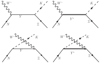
Figure 1: Feynman diagrams for the $\Xi$ production. The intermediate states $Y$ are the ($S=-1$) $\Lambda,\Sigma$ hyperons, and $Y^{*}$ is $\Sigma^{\ast}(1385)$ resonance.

II.1 Non-resonant background

The NRB terms have direct and cross diagrams and the corresponding currents are

$$j^{\mu}_{cc}\big{\arrowvert}_{sY} =\frac{iA_{s}V_{us}}{f_{\pi}}\;\bar{u}_{\Xi}(p^{\prime}_{\Xi})\,\not{p}_{k}\gamma^{5}\frac{\not{p}+\not{q}+M_{Y}}{(p+q)^{2}-M_{Y}^{2}}\Gamma^{\mu}_{NY}\,u_{N}(p)$$

$$j^{\mu}_{cc}\big{\arrowvert}_{uY} =\frac{iA_{u}V_{us}}{f_{\pi}}\;\bar{u}_{\Xi}(p^{\prime}_{\Xi})\,\Gamma^{\mu}_{Y\Xi}\frac{\not{p}-\not{p}_{k}+M_{Y}}{(p-p_{k})^{2}-M_{Y}^{2}}\not{p}_{k}\gamma^{5}\,u_{N}(p)$$

$$\Gamma^{\mu}_{B_{i}B_{j}}(q) =f^{B_{i}B_{j}}_{1}(q^{2})\gamma^{\mu}+if^{B_{i}B_{j}}_{2}(q^{2})\frac{\sigma^{\mu\nu}}{M_{B_{i}}+M_{B_{j}}}q_{\nu}$$

$$-g^{B_{i}B_{j}}_{1}(q^{2})\gamma^{\mu}\gamma^{5}-g^{B_{i}B_{j}}_{3}(q^{2})q^{\mu}\gamma^{5}$$ (7)

where $f_{\pi}$ is the pion decay constant, and $V_{us}(=\sin\theta_{c})$ is the corresponding Cabibbo-Kobayashi-Maskawa (CKM) matrix element for weak strangeness-changing processes. The weak vertex function $\Gamma^{\mu}_{B_{i}B_{j}}(q)$ denotes the weak transition from baryon $B_{i}$ to $B_{j}$ and it is written in terms of transition vector $(f^{B_{i}B_{j}}_{1,2}(q^{2}))$ and axial-vector $(g^{B_{i}B_{j}}_{1,3}(q^{2}))$ form factors. Experimentally, very little information is available regarding these form factors for the weak strangeness-changing transitions between states of the octet baryon. Hence, we rely on exact SU(3) flavor symmetry to relate them to the well-known proton and neutron vector form factors ($f^{p,n}_{1,2}(q^{2})$) and to the nucleon axial-vector one ($g_{A}(q^{2})=g^{np}_{1}(q^{2})$) by using Cabibbo’s theory Cabibbo et al. (2003). The above prescription has also been used by several other authors to obtain $N-Y$ and $Y-Y^{\prime}$ transitions, see for example Refs. Singh and Vicente Vacas (2006); Alam et al. (2015); Adera et al. (2010). In the present work we follow the formalism already presented in Refs. Singh and Vicente Vacas (2006); Alam et al. (2015) and we discuss it here in brief .

Transitions	$C^{BB^{\prime}}_{a}$	$C^{BB^{\prime}}_{s}$
$p\rightarrow p$	1	$\frac{1}{3}$
$n\rightarrow n$	0	$-\frac{2}{3}$
$p\rightarrow n$	1	1
$p\rightarrow\Lambda$	$-\sqrt{\frac{3}{2}}$	$-\frac{1}{\sqrt{6}}$
$p\rightarrow\Sigma^{0}$	$-\frac{1}{\sqrt{2}}$	$\frac{1}{\sqrt{2}}$
$n\rightarrow\Sigma^{-}$	$-$1	1
$\Lambda\rightarrow\Xi^{-}$	$\sqrt{\frac{3}{2}}$	$\frac{-1}{\sqrt{6}}$
$\Sigma^{0}\rightarrow\Xi^{-}$	$\frac{1}{\sqrt{2}}$	$\frac{1}{\sqrt{2}}$
$\Sigma^{+}\rightarrow\Xi^{0}$	1	1

Table 1: SU(3) factors $C^{BB^{\prime}}_{a,s}$ of Eqs. (8) and (9).

II.1.1 Transition form factors for non-resonant background

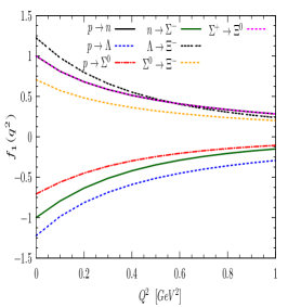
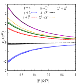
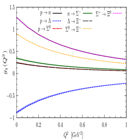
Figure 2: $Q^{2}(=-q^{2})$ dependence of the different transition form factors. Shaded regions show the uncertainties due to SU(3) breaking.

Assuming the octet representation of SU(3) in flavor space, one can relate the vector ($f_{1,2,3}(0)$) and axial-vector couplings ($g_{1,2,3}(0)$) with the reduced matrix elements corresponding to the antisymmetric $({\cal F}^{V,A})$ (also called $f$-type) and symmetric $({\cal D}^{V,A})$ (also called $d$-type) couplings as:

$$f^{BB^{\prime}}_{i}(q^{2})=C^{BB^{\prime}}_{a}{\cal F}^{V}_{i}(q^{2})+C^{BB^{\prime}}_{s}{\cal D}^{V}_{i}(q^{2}),\quad\text{(i=1,2)}$$ (8)

$$g^{BB^{\prime}}_{i}(q^{2})=C^{BB^{\prime}}_{a}{\cal F}^{A}_{i}(q^{2})+C^{BB^{\prime}}_{s}{\cal D}^{A}_{i}(q^{2}),\quad\text{(i=1,3)}$$ (9)

where $C^{BB^{\prime}}_{a,s}$ are related to SU(3) Clebsh-Gordan coefficients. The appearance of two different reduced transition matrix elements ($\mathcal{F}$ and $\mathcal{D}$) between octet baryon states is because of Cabibbo model Cabibbo et al. (2003), which assumes that the vector and axial-vector currents belong to an octet of flavour currents and in the irreducible representation (IR) of $\left\{8\right\}\otimes\left\{8\right\}$, the octet $\left\{8\right\}$ IR appears twice. This means that there are two independent reduced matrix elements when applying the Wigner-Eckart theorem for SU(3) octet transitions through an octet of flavor current operators. One of these reduced matrix elements is related to $\mathcal{F}$ while the other one to $\mathcal{D}$. As the flavour structure for both vector (V) and axial (A) currents remains same, the coefficients $C^{BB^{\prime}}_{a,s}$ given in Table 1 are identical for both currents. It is worth noticing that Eqs. (8) and (9) are generally expressed for the SU(3) couplings. However, it has been shown by previous authors Singh and Vicente Vacas (2006); Alam et al. (2015) that such relationships work well for finite $q^{2}$ too.

The transitions $p\rightarrow p$ and $n\rightarrow n$ can be driven by the electromagnetic current, which is a linear combination of the hypercharge and third component of the isovector currents of the octet of current operators in Cabibbo model Cabibbo et al. (2003). Hence the corresponding Dirac $(f_{1}^{p,n})$ and Pauli $(f_{2}^{p,n})$ form factors appearing when taking matrix elements of the electromagnetic current between proton and neutron states can also be written as in Eq. (8) with the coefficients given in Table 1:

$$f^{n}_{i}(q^{2}) =-\frac{2}{3}{\cal D}^{V}_{i}(q^{2}),\;\;\;\;\$$ i=1,2 (10)

$$f^{p}_{i}(q^{2}) ={\cal F}^{V}_{i}(q^{2})+\frac{1}{3}{\cal D}^{V}_{i}(q^{2}),\;\;\;\ \text{i=1,2}.$$

The system of equations given in (10) is then inverted to give ${\cal D}^{V}_{i}$ and ${\cal F}^{V}_{i}$ in terms of the well-known $f_{i}^{p,n}$ electromagnetic form factors. In this way, all the octet transition vector form factors $f^{BB^{\prime}}_{i}(q^{2})$ can be written uniquely in terms of the proton and neutron form factors. The $q^{2}$-dependence is assumed to be driven by $f_{1,2}^{p,n}(q^{2})$ and no additional $q^{2}$-dependence has been taken. We use Galster’s parameterization Galster et al. (1971) for $f_{1,2}^{p,n}(q^{2})$. The variation of the different transition form factors with $Q^{2}$ are shown in Fig. 2. The shaded region shows the effect due to SU(3) symmetry breaking, see Appendix A for details. We follow the prescription of Ref. Faessler et al. (2008) for SU(3) corrections. We found that among all transition form factors $p\to\Lambda$ transition suffers maximum deviation followed by $n\to\Sigma^{-}$ for both $f_{2}$ and $g_{1}$ form factor while $f_{1}$ form factor (for all transitions) is protected by Ademollo-Gatto theorem Ademollo and Gatto (1964).

Table 2: Constant factors ($A_{s}$, $A_{u}$) in Eqs. (II.1) and (II.2).

Process	Direct term $(A_{s})$			Cross term $(A_{u})$
	$Y=\Lambda$	$Y=\Sigma$	$Y=\Sigma^{\ast}$	$Y=\Lambda$	$Y=\Sigma$	$Y=\Sigma^{\ast}$
$\bar{\nu}_{l}+p\rightarrow l^{+}+K^{+}+\Xi^{-}$	$-\frac{D-3F}{2\sqrt{3}}$	$\frac{D+F}{2}$	$\frac{1}{\sqrt{6}}$	$-\frac{D+3F}{2\sqrt{3}}$	$\frac{D-F}{2}$	$\frac{1}{\sqrt{6}}$
$\bar{\nu}_{l}+p\rightarrow l^{+}+K^{0}+\Xi^{0}$	$-\frac{D-3F}{2\sqrt{3}}$	$-$ $\frac{D+F}{2}$	$-\frac{1}{\sqrt{6}}$	0	$\frac{D-F}{\sqrt{2}}$	$\sqrt{\frac{2}{3}}$
$\bar{\nu}_{l}+n\rightarrow l^{+}+K^{0}+\Xi^{-}$	0	$\frac{D+F}{\sqrt{2}}$	$\sqrt{\frac{2}{3}}$	$-\frac{D+3F}{2\sqrt{3}}$	$-\frac{D-F}{2}$	$-\frac{1}{\sqrt{6}}$

On the other hand, in the axial sector, while ${\cal F}^{A}(0)$ and ${\cal D}^{A}(0)$ still form reduced matrix elements for antisymmetric and symmetric axial couplings with $C^{BB^{\prime}}_{s,a}$ being the same coefficients of Table 1, there is no competing either electromagnetic or weak channel which could be used to fix them separately at finite $q^{2}$, as it was the case for their vector counterparts in Eqs. (10). However, at $q^{2}=0$ some information is available from semileptonic hyperon decays  Cabibbo et al. (2003). Therefore, the extraction of the axial couplings ${\cal F}^{A}(0)$ and ${\cal D}^{A}(0)$ has been performed assuming SU(3) symmetry. For the present work we use the numerical values ${\cal F}^{A}(0)=0.463$ and ${\cal D}^{A}(0)=0.804$ Cabibbo et al. (2003).

For the $q^{2}$-dependence of the octet transition axial form factors, we first express the nucleon axial coupling corresponding to transition $p\to n$ in terms of ${\cal F}^{A}(0)$ and ${\cal D}^{A}(0)$ and relate all of them in terms of ${\cal F}^{A}(q^{2})$ and ${\cal D}^{A}(q^{2})$:

$$g^{np}_{1}(q^{2}) =\frac{g_{A}}{(1-q^{2}/M_{A}^{2})^{2}}$$

$$=\frac{{\cal F}^{A}(0)}{(1-q^{2}/M_{A}^{2})^{2}}+\frac{{\cal D}^{A}(0)}{(1-q^{2}/M_{A}^{2})^{2}}$$

$$={\cal F}^{A}(q^{2})+{\cal D}^{A}(q^{2}).$$ (11)

In the last step we exploit the linear dependence of $g_{A}$ on ${\cal F}^{A}(0)$ and ${\cal D}^{A}(0)$ to write the explicit dependence on $q^{2}$. Therefore, ${\cal F}^{A}(q^{2})$ and ${\cal D}^{A}(q^{2})$ also have the dipole structure (this assumption was also considered in Ref. Singh and Vicente Vacas (2006)). Using Eq. (9), we obtain the other transition form factors in terms of ${\cal F}^{A}(q^{2})$ and ${\cal D}^{A}(q^{2})$. The dipole parameter $M_{A}$ can then be identified as the nucleon axial dipole mass and for present work we take $M_{A}=1.0$ GeV.

Finally, the couplings $A_{s}$ and $A_{u}$ in Eqs. (II.1) are obtained from the SU(3) rotations at strong vertices of the diagrams given in Fig. 1 and are given in Table 2. It is also worth noticing for the reader that we have used pseudo-vector strong couplings at the $BB^{\prime}K$ vertices, as it is obvious from the $\not{p}_{k}\gamma^{5}$ structures appearing in Eqs. (II.1). We have also checked these couplings with the expansion of Chiral Lagrangians at lowest order used in Refs. Rafi Alam et al. (2010); Alam et al. (2012); Rafi Alam et al. (2013b) and found them to be consistent.

II.2 Resonant mechanism

The $K\Xi$ production channel may get contribution from the resonant mechanism as well. However, in absence of experimental data their couplings are not known. To overcome this difficulty we rely again on SU(3) symmetry. Among all the decuplet members only $\Sigma^{\ast}(1385)$ has the right quantum numbers to decay strongly into $K\Xi$ channel. In this section we present the model for resonant mechanism, which is essentially the same as in Ref. Alam et al. (2012).

We start by writing the general expression for the current corresponding to $\Sigma^{\ast}(1385)$ resonance,

$$j^{\mu}_{cc}\big{\arrowvert}_{s\Sigma^{*}} =iA^{\Sigma^{*}}_{s}\frac{\cal C}{f_{\pi}}\;V_{us}\;p_{k}^{\lambda}\;\bar{u}_{\Xi}(p^{\prime}_{\Xi})G_{\lambda\rho}\;(\Gamma_{V}^{\rho\mu}+\Gamma_{A}^{\rho\mu})\;u_{N}(p)$$

$$j^{\mu}_{cc}\big{\arrowvert}_{u\Sigma^{*}} =iA^{\Sigma^{*}}_{u}\frac{\cal C}{f_{\pi}}\;V_{us}\;p_{k}^{\lambda}\;\bar{u}_{\Xi}(p^{\prime}_{\Xi})\;(\tilde{\Gamma}_{V}^{\mu\rho}+\tilde{\Gamma}_{A}^{\mu\rho})\;G_{\rho\lambda}u_{N}(p)$$

$$\tilde{\Gamma}^{\mu\nu}_{i} \equiv\tilde{\Gamma}^{\mu\nu}_{i}(p^{\prime}_{\Xi},q)=\gamma^{0}\left[\Gamma^{\nu\mu}_{i}(p^{\prime}_{\Xi},-q)\right]^{\dagger}\gamma^{0},\quad i=V,A.$$ (12)

The parameter ${\cal C}$ is the decuplet-baryon-meson strong coupling constant appearing below in Eq. (17). It is a free parameter that can be fitted to reproduce the $\Delta(1232)$ decay width. Following Ref. Alam et al. (2012), its numerical value has been taken as $\mathcal{C}\sim 1$.

In Eqs. (II.2), $G^{\mu\nu}(P)$ is the Rarita-Schwinger spin-$3/2$ particle propagator given by:

$$G^{\mu\nu}(P)=\frac{P^{\mu\nu}_{RS}(P)}{P^{2}-M_{\Sigma^{*}}^{2}+iM_{\Sigma^{*}}\Gamma_{\Sigma^{*}}},\qquad$$ (13)

where $P$ is the momentum carried by the resonance: $P=p+q$ for direct terms ($s-$channel), while $P=p-p_{k}=p^{\prime}_{\Xi}-q$ for cross terms ($u-$channel). The operator $P^{\mu\nu}_{RS}$ may be identified as the Rarita-Schwinger Rarita and Schwinger (1941) projection operator,

$$P^{\mu\nu}_{RS}(P)=\sum_{spins}\psi^{\mu}\bar{\psi}^{\nu}=-(\not{P}+M_{\Sigma^{*}})\left[g^{\mu\nu}-\frac{1}{3}\gamma^{\mu}\gamma^{\nu}-\frac{2}{3}\frac{P^{\mu}P^{\nu}}{M_{\Sigma^{*}}^{2}}+\frac{1}{3}\frac{P^{\mu}\gamma^{\nu}-P^{\nu}\gamma^{\mu}}{M_{\Sigma^{*}}}\right].$$ (14)

Finally, the weak vector and axial transition operators $\Gamma^{\alpha\mu}_{V}(p,q)$ and $\Gamma^{\alpha\mu}_{A}(p,q)$ in Eqs. (II.2) are given by Hernandez et al. (2007)

$$\Gamma^{\alpha\mu}_{V}(p,q) = \left[\frac{C_{3}^{V}}{M}\left(g^{\alpha\mu}\not{q}-q^{\alpha}\gamma^{\mu}\right)+\frac{C_{4}^{V}}{M^{2}}\left(g^{\alpha\mu}q\cdot P-q^{\alpha}P^{\mu}\right)+\frac{C_{5}^{V}}{M^{2}}\left(g^{\alpha\mu}q\cdot p-q^{\alpha}p^{\mu}\right)+C_{6}^{V}g^{\mu\alpha}\right]\gamma_{5}$$

$$\Gamma^{\alpha\mu}_{A}(p,q) = \left[\frac{C_{3}^{A}}{M}\left(g^{\alpha\mu}\not{q}-q^{\alpha}\gamma^{\mu}\right)+\frac{C^{A}_{4}}{M^{2}}\left(g^{\alpha\mu}q\cdot P-q^{\alpha}P^{\mu}\right)+C_{5}^{A}g^{\alpha\mu}+\frac{C_{6}^{A}}{M^{2}}q^{\mu}q^{\alpha}\right],$$ (15)

where $C_{i}^{V,A}$ $(i=3-6)$ are $q^{2}$-dependent form factors. Their expressions are taken directly from Ref. Hernandez et al. (2007) for the $n\rightarrow\Delta^{+}$ weak transition with only one exception: we relate $C^{A}_{6}$ with $C^{A}_{5}$ by using partial conservation of the axial current (PCAC) assuming the coupling of the $W^{-}$ boson to the $\Sigma^{\ast}$ resonance through a kaon pole in Fig. 1,

$$C^{A}_{6}(q^{2})=C^{A}_{5}(q^{2})\frac{M^{2}}{m^{2}_{K}-q^{2}}.$$ (16)

In principle, our knowledge of the weak $N\rightarrow\Sigma^{\ast}$ and $\Sigma^{\ast}\rightarrow\Xi$ transition form factors is almost none, as these transitions cannot be driven directly by electromagnetic probes, a research field where the vast majority of associated production studies David et al. (1996); Janssen et al. (2002); Lee et al. (2001); Julia-Diaz et al. (2006); Mart and Sulaksono (2006); Han et al. (2001); Shyam et al. (2010) has been carried out. However, we know that the $\Sigma^{\ast}(1385)$ and $\Delta(1232)$ are members of same decuplet and we can exploit it to relate the $\Sigma^{\ast}(1385)$ transition form factors with other relatively known ones as those of the $N\rightarrow\Delta(1232)$ transition by using again SU(3) symmetry arguments.

We begin writing a Lagrangian describing the interaction between decuplet and octet baryons with meson octet:

$${\cal L}_{dec}={\cal C}\left(\epsilon^{abc}\bar{T}^{\mu}_{ade}u_{\mu,b}^{d}B_{c}^{e}+\,h.c.\right),$$ (17)

where $T^{\mu}$ is the SU(3) representation of the decuplet fields and $a-e$ are the flavor indices. The interaction of baryon octet $(B)$, decuplet and pseudo-scalar meson octet $(\phi(x))$ with external weak/electromagnetic currents is achieved by coupling left $(l_{\mu})$ and right-handed $(r_{\mu})$ external currents in the so-called vielbein $u_{\mu}$:

$$u_{\mu} =i\left[u^{\dagger}(\partial_{\mu}-ir_{\mu})u-u(\partial_{\mu}-il_{\mu})u^{\dagger}\right],$$

$$u^{2}(x) =U(x)=\exp\left(i\frac{\phi(x)}{f_{\pi}}\right)\,.$$ (18)

For further details, the reader is either referred to the review Scherer (2003) or to Refs. Rafi Alam et al. (2010); Alam et al. (2012), where the same formalism has been applied.

In the $WN\to\Delta$ transitions it is well-known that, out of the $8$ form factors appearing in Eq. (II.2), the most dominant contribution comes from $C_{5}^{A}$ (see for example Refs. Lalakulich and Paschos (2005); Hernandez et al. (2007, 2010); Rafi Alam et al. (2016)). The Lagrangian of Eq. (17) only gives information about $C_{5}^{A}(0)$ for all the octet-decuplet baryons’ transitions. Thus, using SU(3) symmetry one can easily relate the weak $(C_{5}^{A}(0))^{B\rightarrow D}$ transition couplings between baryon octet and baryon decuplet with only one of them taken as reference. In our case we chose $(C_{5}^{A}(0))^{n\rightarrow\Delta^{+}}$ as a reference which has been extensively studied in past, see for example Ref. Hernandez et al. (2007). However, given the form of Eqs. (II.2) and (II.2), the SU(3) factors relating the different weak $B\rightarrow D$ transition vertices (given as $\Gamma^{\rho\mu}_{i}$ in Eqs. (II.2)) are totally hidden in our numbers for $A^{\Sigma^{\ast}}_{s,u}$ of Table 2 for the different reactions. Of course, all the other form factors of Eq. (II.2) besides $C_{5}^{A}$ are assumed to rotate equally under SU(3) transformations. The same procedure and assumptions were made previously in Ref. Alam et al. (2012) for the $N\rightarrow\Sigma^{\ast}$ weak transition.

Finally, the energy-dependent width ($\Gamma_{\Sigma^{*}}$) appearing in Eq. (13) may be written as:

$$\Gamma_{\Sigma^{*}}=\Gamma_{N\bar{K}}+\Gamma_{\Lambda\pi}+\Gamma_{\Sigma\pi}+\Gamma_{\Xi K}$$ (19)

where $\Gamma_{B\phi}$ is the partial decay width for a decuplet $(D)$ member to meson $(\phi)$ and baryon octet $(B)$, calculated from the decay amplitude derived from the Lagrangian (17),

$$\Gamma_{D\rightarrow B\phi}=\frac{C_{Y}}{192\pi}\left(\frac{\cal C}{f_{\pi}}\right)^{2}\frac{(W+M_{B})^{2}-m^{2}_{\phi}}{W^{5}}$$

$$\lambda^{3/2}(W^{2},M_{B}^{2},m^{2}_{\phi})\,\Theta(W-M_{B}-m_{\phi}),$$ (20)

where $\lambda(x,y,z)=(x-y-z)^{2}-4yz$ is the Källén lambda function, $\Theta$ is the step function, $M_{B}$ and $m_{\phi}$ are the final baryon and meson masses, respectively, and $W$ is the invariant mass carried by the resonance in the propagator given in Eq.(13), i.e, $W^{2}=P^{2}$. Finally, the factor $C_{Y}$ is 1 for $\Lambda\pi$ and $\frac{2}{3}$ for $N\bar{K}$, $\Sigma\,\pi$ and $\Xi\,K$ partial decay widths, respectively.

III Results

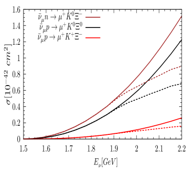
Figure 3: Total cross section $\sigma$ vs. $E_{\nu}$ for the different channels of (II). Dashed lines show the results with $W_{cut}=2.0$ GeV for each process (same color).

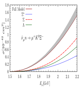
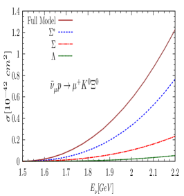
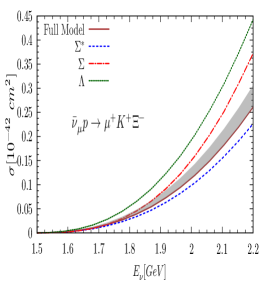
Figure 4: Total cross section $\sigma$ vs. $E_{\nu}$ for the different channels of (II). Shaded regions show effects due to SU(3) breaking.

The total cross sections corresponding to the channels given in (II) are obtained after integrating over $W$ and $Q^{2}$ in Eq. (2). We present the results for muon anti-neutrino induced total cross section in Fig. 3. The full model results are shown by solid curves, while dashed lines show the results by applying a cut in the $K\Xi$ invariant mass of $W_{cut}=2$ GeV for the corresponding processes (identified by the same color). We will discuss the choice of $W_{cut}$ and the effects of it later in this section.

On the other hand, considering the full model, we find that among the three channels $n\to K^{0}\Xi^{-}$ is the most dominant one followed by $p\to K^{0}\Xi^{0}$ and $p\to K^{+}\Xi^{-}$. One should note that if we compare our result(s) for inclusive kaon production with $\Delta S=0$ mechanisms we find that the cross section for $K^{0}$ and $K^{+}$ are about 3 and 6 percent of the corresponding $\Delta S=0$ processes, respectively. This is consonance with the Cabibbo suppression for $|\Delta S|=1$ processes with respect to their $\Delta S=0$ counterparts. For the $\Delta S=0$ kaon production we took the model discussed in Ref. Alam (2014). In their model, they use only non-resonant terms which come from lowest order expansion of chiral Lagrangian. However, in absence of resonant mechanisms, the model is not reliable for high invariant mass and hence the comparison may be treated as guesstimate.

In Fig. 4 we present the contribution due to different intermediate state on the total cross section. Solid lines show again the results of the full model. One can notice that in $\bar{\nu}_{\mu}n\to\mu^{+}K^{0}\Xi^{-}$ and $\bar{\nu}_{\mu}p\to\mu^{+}K^{0}\Xi^{0}$ the contributing diagrams add up, while in $\bar{\nu}_{\mu}p\to\mu^{+}K^{+}\Xi^{-}$ they seem to have strong cancellations due to the interferences, what results in a smaller cross section than the $\Lambda$ and $\Sigma$ term alone.

In fact, all three channels show different behavior regarding their contributing diagrams. Starting from $\bar{\nu}_{\mu}n\to\mu^{+}K^{0}\Xi^{-}$, the most dominating contribution comes from $\Sigma$ term followed by $\Lambda$ and $\Sigma^{\ast}$ resonance. The smaller contribution due to $\Lambda$ term can be understood because of absence of $s-$channel diagram and the larger coupling ($A_{s}=\frac{D+F}{\sqrt{2}}\simeq 0.896$) of the $s-$channel $\Sigma$ current with respect to the coupling of the $\Lambda$ term ($A_{u}=-\frac{D+3F}{2\sqrt{3}}\simeq-0.63$). On the other hand, in this channel $\Sigma^{\ast}$ resonance has the lowest contribution with respect to the others.

The other channel producing $K^{0}$ in the final state is $\bar{\nu}_{\mu}p\to\mu^{+}K^{0}\Xi^{0}$. Unlike the $K^{0}\Xi^{-}$ final state, $\Sigma^{\ast}$ resonance turns out to be the most dominating one followed by $\Sigma$ and $\Lambda$ terms. The dominance of $\Sigma^{\ast}$ comes mainly through its $u-$channel contribution, which moreover has a larger coupling ($\sqrt{\frac{2}{3}}$ vs $-\frac{1}{\sqrt{6}}$) than in the $K^{0}\Xi^{-}$ case. The smallness of the $\Lambda$ contribution can be very easily understood because of the tiny value of its coupling in the $s-$channel ($A_{s}=-\frac{D-3F}{2\sqrt{3}}\simeq 0.169$), the only occurring one. It also seems from inspection of left and middle panels of Fig. 4, and from the numerical values of the couplings given in Table 2 for the $\Sigma$ currents that the interference between $s$ and $u$-channel diagrams is important and destructive for this contribution when both couplings have more similar values.

Finally, in the $\bar{\nu}_{\mu}p\to\mu^{+}K^{+}\Xi^{-}$ reaction, it seems that, due to destructive interference between the contributing diagrams, the cross section gets much reduced. However, in this channel the highest contribution comes from $\Lambda$ term and the $\Sigma^{\ast}$ resonance has the lowest individual contribution.

Nonetheless, it is worth mentioning that in these Cabibbo-suppressed associated production of two strange particles processes, the contribution of $\Sigma^{\ast}(1385)$ resonance is truly important (of the same order than the NRB terms), in contrast to the case of single antikaon production studied in Ref. Alam et al. (2012), where this same resonance was found to play a minor role.

We have also explored the effects due to SU(3) breaking. For this we have considered the model of Ref. Faessler et al. (2008). SU(3) modification in the form factors and the parameterization are given in Appendix A. The corrections have been applied to the form factors appearing in Eq. (II.1), and their effect in cross section is shown by the shaded region in Fig. 4. We observe that in the $\bar{\nu}_{\mu}p\to\mu^{+}K^{0}\Xi^{0}$ channel the effect of SU(3) breaking is negligible, while in channels $\bar{\nu}_{\mu}n\to\mu^{+}K^{0}\Xi^{-}$ and $\bar{\nu}_{\mu}p\to\mu^{+}K^{+}\Xi^{-}$ is about 15 %.

At the higher neutrino energies discussed here, due to availability of phase space, higher ($S=-1$) resonances may contribute. In particular, it seems that the contribution of the $\Lambda(1520)$ can be also very important in the light of Ref. Shyam et al. (2011). However, its inclusion in the present model is beyond the scope of this work.

To check the validity of our model for the analyzed anti-neutrino energy range of this work, we examine the dependence on the invariant mass $W$. We restrict $W$ to remain slightly above the $K\Xi$ threshold and apply a cut in the invariant mass of $W_{cut}=2$ GeV in order to stay as close to threshold as possible. The reason for this is to minimize the effects of higher lying resonances Shyam et al. (2011) not included in our exploratory work. The consequences of this cut on the total cross section are shown in Fig. 3. We observe that at $E_{\nu}=2.2$ GeV, the cross section gets reduced by about 40 percent for $\bar{\nu}_{\mu}n\to\mu^{+}K^{0}\Xi^{-}$ and $\bar{\nu}_{\mu}p\to\mu^{+}K^{0}\Xi^{0}$, while 20 percent for $\bar{\nu}_{\mu}p\to\mu^{+}K^{+}\Xi^{-}$ process. Other advantages of using the low invariant mass kinematic cut comes from the NRB terms, because these have been obtained from the expansion of Chiral Lagrangians at lowest order Rafi Alam et al. (2010); Alam et al. (2012); Scherer (2003) and this kind of expansions are really reliable for low energy and momentum transfers.

Finally, we have also obtained the flux averaged total cross section corresponding to Minerva anti-neutrino flux ($\Phi(E_{\nu})$) as Min ; Aliaga et al. (2016),

$$\langle\sigma\rangle=\frac{\int dE_{\nu}\;\sigma(E_{\nu})\;\Phi(E_{\nu})}{\int dE_{\nu}\Phi(E_{\nu})}\,.$$ (21)

The results thus obtained are presented in Table. 3.

Process	Without Cut	$W_{cut}=2$ GeV
	$10^{-41}$ cm2	$10^{-41}$ cm2
$\bar{\nu}_{\mu}n\to\mu^{+}K^{0}\Xi^{-}$	0.795	0.295
$\bar{\nu}_{\mu}p\to\mu^{+}K^{0}\Xi^{0}$	0.853	0.251
$\bar{\nu}_{\mu}p\to\mu^{+}K^{+}\Xi^{-}$	0.222	0.076

Table 3: Average total cross section convoluted with the anti-neutrino Minerva flux Min ; Aliaga et al. (2016).

We find that the average cross section (without invariant mass cut) for $K^{0}$ production is much higher than for $K^{+}$, in consonance with the larger cross sections for $K^{0}$ production (see Fig. 3). On the other hand, if we observe $\Xi$ hyperon, then both $\Xi^{0}$ and $\Xi^{-}$ have almost similar occurrence. One should notice that if we apply $W_{cut}=2$ GeV, then the average total cross section gets remarkably reduced. Further, the kinematic suppression seems to affect more to $\bar{\nu}_{\mu}p\to\mu^{+}K^{0}\Xi^{0}$ than $\bar{\nu}_{\mu}n\to\mu^{+}K^{0}\Xi^{-}$.

Although the total cross sections for the reactions studied in this work are normally between one and two orders of magnitude below those studied in Ref. Rafi Alam et al. (2010) for single kaon production off nucleons, the convoluted total cross sections (even with the invariant mass cut) with the anti-neutrino Minerva flux (shown in Table 3) are of the same order of magnitude as those shown in Table II of Rafi Alam et al. (2010) calculated with different muon neutrino fluxes corresponding to ANL Barish et al. (1977), MiniBooNE Aguilar-Arevalo et al. (2010) and T2K Abe et al. (2013) experiments.

The explanation for this apparent contradiction is not difficult to understand: the cross sections studied in Ref. Rafi Alam et al. (2010) had a quite lower energy threshold than these for $K\Xi$ production ($0.8$ GeV vs $1.5$ GeV, respectively), and the fluxes used in Rafi Alam et al. (2010) had a significant contribution also at lower neutrino energies ($E_{\nu}\sim 0.8$ GeV) and shorter high energy tails, oppositely to the Minerva flux, which is peaked at $E_{\nu}\sim 3.5$ GeV and has a much longer tail extending towards higher energies. The fluxes used in Ref. Rafi Alam et al. (2010) had their significant contribution in an energy range where the $KN$ production reactions also had a sizable cross section, and they fell off faster than the Minerva flux. Therefore, at the end the weighted cross section given by Eq. (21) gives similar results in both cases (Table II of Ref. Rafi Alam et al. (2010) and Table 3 of this work). This is just a consequence of the fact that the product $\sigma(E_{\nu})\,\Phi(E_{\nu})$ is sizable in an energy range where the $KN$ and the $K\Xi$ cross sections reach similar values with different fluxes. Another reason to apply the kinematic cut $W_{cut}$ here is to avoid reaching invariant masses far larger than $2$ GeV when flux-averaging the cross sections with a high energy flux such as that of Minerva experiment. In this way we are sure that the effects coming from contributing higher resonances not included in our model are avoided as much as possible, and therefore we are using our model only in the region of invariant masses where we think it to be more reliable.

Given the numbers of the second column of Table 3, and the conclusions for the similar numbers given in Ref. Rafi Alam et al. (2010), we think that the reactions (II) could be observed with current measurement facilities such as Minerva experiment.

IV Conclusions

In this work we have obtained the cross sections for Cabibbo-suppressed associated $K\Xi$ production through charge current interactions induced by anti-neutrinos. The present work represents the first attempt to estimate the cross sections for production of $S=-2$ baryons in weak processes. These processes are not feasible in neutrino mode.

The model is a natural continuation of that used by the same authors in Refs. Rafi Alam et al. (2010); Alam et al. (2012); Rafi Alam et al. (2013b). It contains Born (NRB) terms driven by the propagation of strange ($\Lambda$,$\Sigma$) octet baryons, and also the lowest lying strange resonance of the decuplet, namely the $\Sigma^{\ast}(1385)$, which is found to play a very significant role in these reactions, contrarily to the case of $\bar{K}N$ production discussed in Ref. Alam et al. (2012).

In a recent work Shyam et al. (2011), a diagrammatically-inspired model like that used here has shown that the inclusion of higher lying strange resonances like the $\Lambda(1520)$ is very important to describe the $K^{-}p\rightarrow K\Xi$ production data. Although the inclusion of the $\Lambda(1520)$ is out of the scope of this article, we do not renounce including it in future refinements of the present exploratory work in the light of the findings of Ref. Shyam et al. (2011).

The simplicity of the present model makes it possible to be implemented in the present Monte Carlo Generators like GENIE Andreopoulos et al. (2010, 2015). The cross sections computed here are about one order of magnitude less than the corresponding $\Delta S=0$ associated $K$ production mechanism. However, they are measurable at the current neutrino facilities like Minerva and in the proposed mega-detectors like Dune Acciarri et al. (2015) and Hyper-Kamiokande Nakamura (2003).

Appendices

A SU(3) Breaking

Following Ademollo and Gatto (1964), we write the effective Lagrangian which includes additional couplings $H_{i}$ $(i=1\cdots 4)$ describing SU(3) breaking as:

$${\mathcal{L}}_{1} =D\,\langle\bar{B}\Gamma^{\mu}\{\epsilon_{\mu},B\}\rangle\,+\,F\,\langle\bar{B}\Gamma^{\mu}[\epsilon_{\mu},B]\rangle$$

$$+\frac{H_{1}}{\sqrt{3}}\,\langle\bar{B}\Gamma^{\mu}B\{\epsilon_{\mu},\lambda_{8}\}\rangle+\frac{H_{2}}{\sqrt{3}}\,\langle\bar{B}\Gamma^{\mu}\{\epsilon_{\mu},\lambda_{8}\}B\rangle$$

$$+\frac{H_{3}}{\sqrt{3}}\,\langle\bar{B}\Gamma^{\mu}\epsilon_{\mu}B\lambda_{8}-\bar{B}\Gamma^{\mu}\lambda_{8}B\epsilon_{\mu}\rangle$$

$$+\frac{H_{4}}{\sqrt{3}}\,\biggl{(}\,\langle\bar{B}\epsilon_{\mu}\rangle\Gamma^{\mu}\langle B\lambda_{8}\rangle+\langle\bar{B}\lambda_{8}\rangle\Gamma^{\mu}\langle B\epsilon_{\mu}\rangle\,\biggr{)}$$ (A1)

where $B$ and $\epsilon_{\mu}$ are the octet of baryon fields and the external current, respectively. Angular braces, $\langle\cdots\rangle$, represent the trace of matrices in flavor space and $\lambda_{8}$ is the $8^{th}$ component of the set of Gell-Mann matrices. Finally, depending upon the nature of the current, $\Gamma^{\mu}$ can be read as $\gamma^{\mu}$ or $\gamma^{\mu}\gamma^{5}$ for vector and axial-vector cases, respectively.

The couplings of baryons are then expressed in terms of the constants $D$, $F$ and $H_{i}$ as Faessler et al. (2008):

$${\cal F}^{np} =D+F+\frac{2}{3}(H_{2}-H_{3})\,,$$

$${\cal F}^{\Lambda p} =-\sqrt{\frac{3}{2}}\biggl{(}F+\frac{D}{3}+$$

$$\frac{1}{9}(H_{1}-2H_{2}-3H_{3}-6H_{4})\biggr{)}\,,$$

$${\cal F}^{\Sigma^{-}n} =D-F-\frac{1}{3}(H_{1}+H_{3})\,,$$

$${\cal F}^{\Lambda\Xi^{-}} =-\sqrt{\frac{3}{2}}\biggl{(}-F+\frac{D}{3}+$$

$$\frac{1}{9}(-2H_{1}+H_{2}+3H_{3}-6H_{4})\biggr{)}\,,$$

$${\cal F}^{\Sigma^{+}\Xi^{0}} =D+F-\frac{1}{3}(H_{2}-H_{3})\,,$$

$${\cal F}^{\Sigma^{0}p} =\frac{1}{\sqrt{2}}{\cal F}^{\Sigma^{-}n}\,,$$

$${\cal F}^{\Sigma^{0}\Xi^{-}} =\frac{1}{\sqrt{2}}{\cal F}^{\Sigma^{+}\Xi^{0}}\,.$$

Note that terms proportional to couplings $D$ and $F$ are SU(3) symmetric, while couplings $H_{1-4}$ account for possible symmetry breaking effects. Explicit values of coupling parameters $D,F$ and $H_{i}$ are taken from Ref. Faessler et al. (2008).

$$D =0.7505\qquad F=0.5075$$

$$H_{1}^{g_{1}} =-0.050\qquad H_{2}^{g_{1}}=0.011$$

$$H_{3}^{g_{1}} =-0.006\qquad H_{4}^{g_{1}}=0.037$$

$$H_{1}^{f_{2}} =-0.246{\mathcal{X}}\qquad H_{2}^{f_{2}}=0.096{\mathcal{X}}$$

$$H_{3}^{f_{2}} =0.021{\mathcal{X}}\qquad H_{4}^{f_{2}}=0.030{\mathcal{X}},$$

where ${\mathcal{X}}=\frac{M+M_{Y}}{M}$ is a constant appearing because of different normalization convention taken for $f_{2}$ form factor in Ref. Faessler et al. (2008) and in present case (see Eq. (II.1)). Further assumptions taken are:

1. The vector coupling $f_{1}(0)$ does not receive any correction due to SU(3) breaking because it is protected against these effects by the Ademollo-Gatto theorem Ademollo and Gatto (1964).

2. Second class currents ($f_{3},\,g_{2}$), which have opposite sign under $G-$parity transformation if compared to first class currents ($f_{1,2},\,g_{1,3}$), are ignored. We show only first class currents in Eq. (II.1).

3. For $q^{2}$ dependence of the breaking parameters ($H_{i}^{g_{1},f_{2}}$), we assume a dipole form with dipole parameter taken as $M_{A}(M_{V})$ for axial(vector) form factors, respectively.

4. We assume that the PCAC and Goldberger-Treiman relation is valid even when $g_{1}$ receives SU(3) corrections. Further, $g_{3}$ will get modified from $g_{1}$. In particular, PCAC and kaon-pole dominance implies the substitution $g^{B_{i}B_{j}}_{3}(q^{2})\rightarrow-g^{B_{i}B_{j}}_{1}(q^{2})\frac{\not{q}}{q^{2}-M^{2}_{K}}$ in eq. (II.1). This replacement has been made for all the calculations presented in this work.

Finally, care should be taken while using the values for $D$ and $F$. In our numerical calculations we used non-breaking couplings as $D=0.804$ and $F=0.463$ Cabibbo et al. (2003). However, in order to be consistent with Ref. Faessler et al. (2008) we use their parameters for SU(3) breaking calculations.

References

- Alvarez-Ruso et al. (2014) L. Alvarez-Ruso, Y. Hayato, and J. Nieves, New J.Phys. 16, 075015 (2014), arXiv:1403.2673 [hep-ph] .
- Katori and Martini (2018) T. Katori and M. Martini, J.Phys. G45, 013001 (2018), arXiv:1611.07770 [hep-ph] .
- Singh and Vicente Vacas (2006) S. Singh and M. Vicente Vacas, Phys.Rev. D74, 053009 (2006).
- Alam et al. (2015) M. Alam, M. Athar, S. Chauhan, and S. Singh, J.Phys. G42, 055107 (2015), arXiv:1409.2145 [hep-ph] .
- Wu and Zou (2015) J.-J. Wu and B.-S. Zou, Few Body Syst. 56, 165 (2015), arXiv:1307.0574 [hep-ph] .
- Sobczyk et al. (2019) J. Sobczyk, N. Rocco, A. Lovato, and J. Nieves, (2019), arXiv:1901.10192 [nucl-th] .
- Rafi Alam et al. (2013a) M. Rafi Alam, S. Chauhan, M. Sajjad Athar, and S. Singh, Phys.Rev. D88, 077301 (2013a), arXiv:1310.7704 [nucl-th] .
- Fatima et al. (2019) A. Fatima, M. S. Athar, and S. Singh, Front.in Phys. 7, 13 (2019), arXiv:1807.08314 [hep-ph] .
- Farooq (7 29) S. Farooq, Antineutrino-induced charge current quasi-elastic neutral hyperon production in ArgoNeuT, Ph.D. thesis, Kansas State U. (2016-07-29).
- (10) “Minerva,” https://minerva.fnal.gov/.
- (11) “Microboone,” https://microboone.fnal.gov/.
- (12) “Nova,” https://novaexperiment.fnal.gov/.
- (13) “Argoneut,” https://t962.fnal.gov/.
- Andreopoulos et al. (2010) C. Andreopoulos et al., Nucl.Instrum.Meth. A614, 87 (2010), arXiv:0905.2517 [hep-ph] .
- Hayato (2009) Y. Hayato, Neutrino interactions: From theory to Monte Carlo simulations. Proceedings, 45th Karpacz Winter School in Theoretical Physics, Ladek-Zdroj, Poland, February 2-11, 2009, Acta Phys. Polon. B40, 2477 (2009).
- (16) “Nuwro - wroclaw neutrino event generator,” http://borg.ift.uni.wroc.pl/nuwro/.
- (17) “Gibuu - the giessen boltzmann-uehling-uhlenbeck project.” https://gibuu.hepforge.org/trac/wiki.
- Rafi Alam et al. (2010) M. Rafi Alam, I. Ruiz Simo, M. Sajjad Athar, and M. Vicente Vacas, Phys.Rev. D82, 033001 (2010), arXiv:1004.5484 [hep-ph] .
- Alam et al. (2012) M. Alam, I. Simo, M. Athar, and M. Vicente Vacas, Phys.Rev. D85, 013014 (2012), arXiv:1111.0863 [hep-ph] .
- Faessler et al. (2008) A. Faessler, T. Gutsche, B. R. Holstein, M. A. Ivanov, J. G. Korner, and V. E. Lyubovitskij, Phys.Rev. D78, 094005 (2008), arXiv:0809.4159 [hep-ph] .
- Cabibbo et al. (2003) N. Cabibbo, E. C. Swallow, and R. Winston, Ann.Rev.Nucl.Part.Sci. 53, 39 (2003).
- Adera et al. (2010) G. Adera, B. Van Der Ventel, D. van Niekerk, and T. Mart, Phys.Rev. C82, 025501 (2010), arXiv:1112.5748 [nucl-th] .
- Weinberg (1958) S. Weinberg, Phys.Rev. 112, 1375 (1958).
- Fatima et al. (2018) A. Fatima, M. Sajjad Athar, and S. Singh, Phys.Rev. D98, 033005 (2018), arXiv:1806.08597 [hep-ph] .
- Galster et al. (1971) S. Galster, H. Klein, J. Moritz, K. Schmidt, D. Wegener, and J. Bleckwenn, Nucl.Phys. B32, 221 (1971).
- Ademollo and Gatto (1964) M. Ademollo and R. Gatto, Phys.Rev.Lett. 13, 264 (1964).
- Rafi Alam et al. (2013b) M. Rafi Alam, I. Ruiz Simo, M. Sajjad Athar, and M. Vicente Vacas, Phys.Rev. D87, 053008 (2013b), arXiv:1211.4947 [hep-ph] .
- Rarita and Schwinger (1941) W. Rarita and J. Schwinger, Phys.Rev. 60, 61 (1941).
- Hernandez et al. (2007) E. Hernandez, J. Nieves, and M. Valverde, Phys.Rev. D76, 033005 (2007).
- David et al. (1996) J. David, C. Fayard, G. Lamot, and B. Saghai, Phys.Rev. C53, 2613 (1996).
- Janssen et al. (2002) S. Janssen, J. Ryckebusch, D. Debruyne, and T. Van Cauteren, Phys.Rev. C65, 015201 (2002).
- Lee et al. (2001) F. Lee, T. Mart, C. Bennhold, and L. Wright, Nucl.Phys. A695, 237 (2001).
- Julia-Diaz et al. (2006) B. Julia-Diaz, B. Saghai, T.-S. Lee, and F. Tabakin, Phys.Rev. C73, 055204 (2006).
- Mart and Sulaksono (2006) T. Mart and A. Sulaksono, Phys.Rev. C74, 055203 (2006).
- Han et al. (2001) B. S. Han, M. K. Cheoun, K. Kim, and I.-T. Cheon, Nucl.Phys. A691, 713 (2001).
- Shyam et al. (2010) R. Shyam, O. Scholten, and H. Lenske, Phys.Rev. C81, 015204 (2010), arXiv:0911.3351 [hep-ph] .
- Scherer (2003) S. Scherer, Adv. Nucl. Phys. 27, 277 (2003), arXiv:hep-ph/0210398 [hep-ph] .
- Lalakulich and Paschos (2005) O. Lalakulich and E. A. Paschos, Phys.Rev. D71, 074003 (2005).
- Hernandez et al. (2010) E. Hernandez, J. Nieves, M. Valverde, and M. Vicente Vacas, Phys.Rev. D81, 085046 (2010), arXiv:1001.4416 [hep-ph] .
- Rafi Alam et al. (2016) M. Rafi Alam, M. Sajjad Athar, S. Chauhan, and S. K. Singh, Int. J. Mod. Phys. E25, 1650010 (2016), arXiv:1509.08622 [hep-ph] .
- Alam (2014) M. R. Alam, Weak Production of K and Mesons off the Nucleon, Ph.D. thesis, Aligarh Muslim U. (2014).
- Shyam et al. (2011) R. Shyam, O. Scholten, and A. Thomas, Phys.Rev. C84, 042201 (2011), arXiv:1108.2318 [hep-ph] .
- Aliaga et al. (2016) L. Aliaga et al. (MINERvA), Phys.Rev. D94, 092005 (2016), arXiv:1607.00704 [hep-ex] .
- Barish et al. (1977) S. Barish et al., Phys.Rev. D16, 3103 (1977).
- Aguilar-Arevalo et al. (2010) A. Aguilar-Arevalo et al. (MiniBooNE), Phys.Rev. D81, 092005 (2010), arXiv:1002.2680 [hep-ex] .
- Abe et al. (2013) K. Abe et al. (T2K), Phys.Rev. D87, 012001 (2013), arXiv:1211.0469 [hep-ex] .
- Andreopoulos et al. (2015) C. Andreopoulos et al., (2015), arXiv:1510.05494 [hep-ph] .
- Acciarri et al. (2015) R. Acciarri et al. (DUNE), (2015), arXiv:1512.06148 [physics.ins-det] .
- Nakamura (2003) K. Nakamura, Neutrinos and implications for physics beyond the standard model. Proceedings, Conference, Stony Brook, USA, October 11-13, 2002, Int. J. Mod. Phys. A18, 4053 (2003), [,307(2003)].