Global Thermodynamics for Heat Conduction Systems

Abstract

We propose the concept of global temperature for spatially non-uniform heat conduction systems. With this novel quantity, we present an extended framework of thermodynamics for the whole system such that the fundamental relation of thermodynamics holds, which we call “global thermodynamics” for heat conduction systems. Associated with this global thermodynamics, we formulate a variational principle for determining thermodynamic properties of the liquid-gas phase coexistence in heat conduction, which corresponds to the natural extension of the Maxwell construction for equilibrium systems. We quantitatively predict that the temperature of the liquid-gas interface deviates from the equilibrium transition temperature. This result indicates that a super-cooled gas stably appears near the interface.

1 Introduction

The behavior of liquids and gases close to equilibrium have been extensively studied for a long time. As a macroscopic universal theory describing these phases of matter, hydrodynamics is believed to be well-established Landau-Lifshitz-Fluid , and the connection of the hydrodynamics with the classical and quantum mechanics of atoms have been discussed for over a century Zubarev ; Mclennan . Nevertheless, in this paper, we construct a new universal theory for thermodynamic properties in the linear response regime. There are two main messages. First, a new concept, global temperature, is found, with which a novel framework of global thermodynamics is constructed to describe the whole of non-uniform non-equilibrium systems with local equilibrium thermodynamics. This outcome provides a fresh viewpoint for the description of systems out of equilibrium. Second, this formulation provides non-trivial quantitative predictions. As an example, let us consider pure water under a pressure of $p^{\mathrm{ex}}=1.013\times 10^{5}$ Pa, where two heat baths of temperature $T_{1}=368.0$ K and $T_{2}=378.0$ K are in contact with the sides of the system. See Fig. 1 for an illustration. Recall that the liquid-gas transition temperature is $373.1$ K. Based on global thermodynamics, in this paper, we predict that the interface temperature of the liquid-gas coexistence is $368.3$ K. This result means that super-cooled gas stably appears in heat conduction, which may be tested in experiments.

In the remaining part of this introduction, we first present a brief summary of development in non-equilibrium statistical mechanics, confirming that the phenomenon described above has never been discussed by established theories. We then provide a review of extended frameworks of thermodynamics so that readers can understand how the global thermodynamics proposed in this paper is different from previous frameworks. At the end of the introduction, we summarize the achievements of this paper.

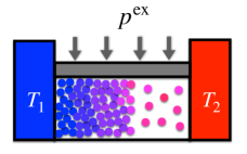
Figure 1: Example of the system under study.

1.1 Non-equilibrium statistical mechanics

In the universal theory of macroscopic irreversible dynamics built by Onsager, a steady-state current is assumed to be linear in the thermodynamic forces Onsager1931 . The linear coefficients form a non-negative symmetric matrix, which is referred to as the Onsager matrix. This theory with a variational principle for determining a current and/or a thermodynamic force is called irreversible thermodynamics, which is valid near equilibrium Groot-Mazur . Onsager theory can be interpreted as a universal theory for the dynamical fluctuations of thermodynamic variables, where the properties of the Onsager matrix are connected to the stability of the equilibrium state and the time-reversal symmetry in microscopic systems. In short, this fluctuation theory is represented by a simple stochastic process with a symmetry property Onsager1931 ; Schmitz . In accordance with this theory, statistical mechanics of trajectories has been studied based on microscopic dynamics, which leads to the expression of probability densities, linear and non-linear response formulas, and macroscopic deterministic dynamics Zubarev ; Mclennan ; Kubo ; Nakano ; Zwanzig ; Mori ; Kawasaki-Gunton .

After these developments, in the last two decades, our understanding of phenomena related to thermodynamics has progressed greatly because of the following two reasons. First, the development of experimental techniques for the measurement and manipulation of biological molecular machines Ashkin ; Bustamante ; Svoboda ; Chu ; Noji naturally leads to the extension of thermodynamics to mesoscopic scales, which is now called stochastic thermodynamics SeifertRPP ; Sekimoto-book ; Kalges-Just-Jarzynski . Second, the newly discovered relations, such as the fluctuation theorem Evans-Cohen-Morriss and the Jarzynski equality JarzynskiPRL , have emerged as universal Gallavotti ; Kurchan ; LS ; Maes ; Crooks ; JarzynskiDFT , providing a new starting point for the re-organization of previous theories with greatly simplified derivations of the formulas CrooksNRL ; KN ; KNST-rep ; Maes-rep ; SasaFluid . These two developed directions, stochastic thermodynamics and new universal relations, are related to each other and have given rise to a new connection with large deviation theory Bodineau-Derrida ; BertiniETAL ; Maes-LD ; Nemoto ; Bertini-rev , and information theory Information .

These results are quite useful when we specify a phenomenon under study. Indeed, the phase coexistence in heat conduction can be studied through a tough calculation based on the non-equilibrium statistical mechanics SNIN . However, we could not conjecture the non-trivial nature of this phenomenon immediately from principles of non-equilibrium statistical mechanics. For example, although one expects a variational formulation for the phase coexistence in heat conduction by recalling the minimum entropy production principle min-ent , we cannot obtain thermodynamic properties directly from the principle because the variational principle basically determines the statistical ensemble in the linear response regime as the minimizer of the entropy production Klein . In order to develop a variational principle for thermodynamic quantities, we have to start with an extended framework of thermodynamics.

1.2 Extended frameworks of thermodynamics

Equilibrium thermodynamics provides a unified description of thermodynamic properties of materials at equilibrium. It also formalizes the second law, which leads to a variational principle for determining equilibrium states Callen ; Prigogine-Kondepudi . The variational principle naturally suggests the law of fluctuation of thermodynamic variables Einstein , which is formulated as a large deviation theory. From this viewpoint, a framework of statistical mechanics may be constructed in a consistent manner with the fluctuation theory of thermodynamic variables Oono .

Therefore, in order to establish a universal theory for thermodynamic properties out of equilibrium, it is natural to consider an extended framework of thermodynamics. A naive attempt is to extend the equilibrium fundamental relation of thermodynamics

$$dF=-SdT-pdV$$ (1.1)

for the case of simple fluids, where $F$ is the Helmholtz free energy and $S$ is the entropy. Examples of such attempts can be seen in Refs. Keizer ; Eu ; Jou-book . The heart of the problem for the extension is to confirm the two conditions: First, the theory is self-consistent and self-contained; second, new predictions specific to the extension are presented. However, the two conditions are not confirmed in many studies. The derivation of the extended thermodynamics from the microscopic theory, regardless of its importance, does not make sense unless the extended framework satisfies the above two conditions. Here, we do not give a complete review of previous studies on the extended framework of thermodynamics, but study heat conduction systems from the viewpoint of the extended framework of thermodynamics.

Heat conduction is described as a spatially extended system in which thermodynamic variables slowly vary in space. The local subsystems, which are small but macroscopic, are regarded as a local equilibrium state Landau-Lifshitz-Fluid ; Groot-Mazur ; Bedeauz86 . If we followed this standard description, we could not have a strong motivation to seek a thermodynamic framework because all thermodynamic properties can be calculated by the heat conduction equation and the local equilibrium thermodynamics. Nevertheless, we still have two possibilities for considering an extended framework of thermodynamics.

The first attempt is to go beyond the local equilibrium thermodynamics. In this approach, which may be adapted in Refs. Jou ; Sasa-Tasaki , the equation of state for the local subsystems is modified to contain the influence of the heat flux. Since such a contribution is quite small in the linear response regime, the theory is not useful even if it is correct. Although this approach may still be effective for spatially homogeneous driven systems, in which intensive parameters may describe the balance of extensive variables Sasa-Tasaki ; Hayashi-Sasa ; Bertin ; Seifert-contact ; Dickman , we do not deal with such systems in this paper.

In the second approach, we retain the standard description for a spatially extended system with local equilibrium thermodynamics. On this basis, we then seek a thermodynamic framework for the whole system. As an example, we first consider the extension of the second law, by which a state variable “entropy” is defined, and we then derive the thermodynamic relation which corresponds to an extension of the fundamental relation of thermodynamics. A concrete procedure of the first step was proposed by introducing the concept of excess heat Jou-book ; Landauer ; Oono-Paniconi . This idea was also studied from semi-macroscopic and microscopic theories Hatano-Sasa ; Ruelle ; KNST ; NN ; Jona-thermo ; Maes-thermo ; Spinney-Ford . However, the fundamental relation of thermodynamics has not been derived from the extended entropy. One reason may be that an interesting phenomenon associated with the extended entropy was not addressed. Nevertheless, one can continue to seek a possible framework without considering certain phenomena. Indeed, for a specific model of heat conduction, the extended entropy was numerically estimated Chiba-Nakagawa , which suggests that the extended entropy is close to the spatial integration of the local equilibrium entropy density. Since the extended entropy can be obtained in experiments, a natural question is “What is temperature?” If the fundamental relation of thermodynamics is formulated, there should be a temperature satisfying it. We consider this question seriously, putting aside specific phenomena.

1.3 Summary of results

We first focus on single-phase systems (either liquid or gas) in heat conduction. By assuming local equilibrium thermodynamics, we define the entropy $S$ and the Helmholtz free energy $F$ in heat conduction by the spatial integration of the local density fields corresponding to these variables. The pressure field $p$ is homogeneous in space. Then, the problem is to find a temperature ${\tilde{T}}$ satisfying the fundamental relation

$$dF=-Sd{\tilde{T}}-pdV$$ (1.2)

in the linear response regime. In §3, we solve this problem by defining $\tilde{T}$ as the kinetic temperature averaged over particles in the system. We call this temperature global temperature. It should be noted that the local temperature $T(\bm{r})$, which depends on the position $\bm{r}$, satisfies the thermodynamic relations for each point $\bm{r}$. In contrast to the local relations, (1.2) is a global relation applied for the whole system as if the system is at equilibrium. We call such a thermodynamic framework global thermodynamics. This formulation is also interpreted as a mapping of each heat conduction system to an equilibrium system through the novel quantity of the global temperature, $\tilde{T}$.

The formulation for a single-phase system is indeed derived from fluid dynamics with local equilibrium thermodynamics. That is, this formulation is interpreted as a different formulation for describing thermodynamic quantities in the linear response regime. The prediction by using global thermodynamics can also be predicted by hydrodynamics with local equilibrium thermodynamics, in principle. Here, we go one step further. We consider a thermodynamic phenomenon that cannot be described by the standard hydrodynamics with local equilibrium thermodynamics. This is the phenomenon of phase coexistence in heat conduction. In §4, we study this phenomenon and we show how existing theories are not appropriate for determining the thermodynamic properties. The essential point is that the condition for the connection of the two phases is outside of the local equilibrium thermodynamics.

We study the phase coexistence in heat conduction with the framework of global thermodynamics. We first formulate a variational principle for determining the local temperature of the liquid-gas interface. The idea is quite simple. Fixing the global temperature of the whole system, we naturally extend the variational principle for equilibrium systems to that for heat conduction systems. This idea was proposed in our previous paper NS . Remarkably, by using the solution of the variational equation, in §5, we derive a universal relation among the interface temperature $\theta$, the equilibrium transition temperature $T_{\mathrm{c}}$, the global temperature ${\tilde{T}}$, and the mean temperature of the two heat baths $T_{\mathrm{m}}$, which is

$$\theta-T_{\mathrm{c}}={\tilde{T}}-T_{\mathrm{m}}.$$ (1.3)

We call this relation the temperature relation. From the temperature relation, we find that the temperature of the liquid-gas interface deviates from the equilibrium transition temperature. That is, super-cooled gas stably appears near the interface in heat conduction. This is a qualitatively new phenomenon that has never been considered in previous studies.

Since the steady state as determined by the variational principle is expressed as a function of the global temperature, the prediction of measurable quantities for given conditions is indirect. Thus, in §6, we re-express all quantities in the steady state in terms of the two temperatures of the heat baths. We present several formulas of the interface temperature by directly using measurable quantities. Furthermore, we illustrate examples of quantitative results for a van der Waals fluid and pure water.

For the steady state determined by the variational principle, we further develop thermodynamics for heat conduction systems with phase coexistence. First, in §7, we derive the fundamental relation associated with the Gibbs free energy $G$. At first sight, the result does not seem to contain non-equilibrium extensions. This is because $G$ is not differentiable at the transition point at equilibrium. By performing a careful analysis near equilibrium, we find that the fundamental relation holds in an appropriate equilibrium limit. The heat capacity and the compressibility, which are singular at equilibrium, are also obtained as a regularized form while breaking the additivity. In §8, we derive the fundamental relation associated with the Helmholtz free energy $F$. Since the free energy $F$ is defined for the coexistence phase in equilibrium cases, its non-equilibrium extension can be written as a perturbation from the equilibrium form. We derive this expression explicitly.

It should be noted that the quantitative prediction is made based on a fundamental assumption of the variational principle. As is often observed in universal theories, one may replace the fundamental assumption by another one. In §9, we formulate the theory starting from assumptions other than the variational principle. For example, when we assume the fundamental relation of thermodynamics for the whole system by using the global temperature, we can derive the results of the variational principle. As another example, one may focus on how the volume change near the transition temperature at constant pressure exhibits the singularity in the equilibrium limit. Supposing the simplest form of a singularity, we can derive the results of the variational principle. These findings indicate that the theory itself possesses an elegant structure.

In §10, we extend the theory in §3 to cover steady states with an arbitrarily shaped container beyond the linear response regime, while restricting our attention to single-phase systems. Our theory quantitatively predicts a new relation among the global quantities in this setup.

2 Preliminaries

2.1 Equilibrium thermodynamics

We consider a macroscopic material at equilibrium. As the simplest example, we focus on a simple fluid whose thermodynamic state is characterized by temperature $T$, the volume $V$ of a container, and the amount of material $N$. For a system in contact with a heat bath of temperature $T$ which may be controlled externally, there exists a state variable $S(T,V,N)$, called entropy, which satisfies the Clausius equality

$$dS=\frac{d^{\prime}Q}{T}$$ (2.1)

for infinitesimal quasi-static heat $d^{\prime}Q$ from the heat bath. The infinitesimal change of internal energy $U(T,V,N)$ of the material is determined by

$$dU=d^{\prime}Q+d^{\prime}W,$$ (2.2)

which is referred to as the first law of thermodynamics. $d^{\prime}W$ is the infinitesimal quasi-static work required in the infinitesimal change of the volume $dV$, which is given by

$$d^{\prime}W=-pdV.$$ (2.3)

The substitution of (2.1) and (2.3) into (2.2) leads to the fundamental relation of thermodynamics:

$$dU=TdS-pdV.$$ (2.4)

From this expression, we find that it is useful to consider $U$ as a function of $(S,V,N)$. Indeed, a single function $U(S,V,N)$ leads to all thermodynamic properties such as equation of state

$$p=p(T,V,N)$$ (2.5)

and heat capacity

$$C_{V}=C_{V}(T,V,N).$$ (2.6)

We then define chemical potential $\mu$ as

$$\mu\equiv\left({\frac{\partial U}{\partial N}}\right)_{S,V}.$$ (2.7)

Various thermodynamic functions equivalent to $U(S,V,N)$ can be defined by the Legendre transformation of $U(S,V,N)$:

$$F(T,V,N) \equiv \min_{S}[U(S,V,N)-TS],$$ (2.8)

$$H(S,p,N) \equiv \min_{V}[U(S,V,N)+pV].$$ (2.9)

$$G(T,p,N) \equiv \min_{S}[H(S,p,N)-TS].$$ (2.10)

The fundamental relations associated with these functions are

$$dF=-SdT-pdV+\mu dN,$$ (2.11)

$$dH=TdS+Vdp+\mu dN,$$ (2.12)

$$dG=-SdT+Vdp+\mu dN.$$ (2.13)

Substituting $G(T,p,N)=NG(T,p,1)$ into (2.13), we find

$$G=\mu N.$$ (2.14)

This form together with (2.13) leads to the Gibbs-Duhem relation

$$-SdT+Vdp-Nd\mu=0.$$ (2.15)

The extensivity of thermodynamic quantity leads to the concept of density defined as the quantity per unit volume, similarly to particle density $\rho=N/V$. For instance, entropy density is defined as

$$s(T,\rho)\equiv\frac{S(T,V,N)}{V}.$$ (2.16)

By using $\rho=\rho(T,p)$, which is obtained from (2.5), one may consider the entropy density as a function of $(T,p)$, which is expressed as

$$s(T,p)=s(T,\rho(T,p)),$$ (2.17)

following the convention in thermodynamics. Similarly to the entropy density, for any extensive quantity $A$, its density is defined as

$$a(T,\rho)\equiv\frac{A(T,V,N)}{V},$$ (2.18)

$$a(T,p)=a(T,\rho(T,p)).$$ (2.19)

We here consider free energy density $g=G/V$. Substituting $G=gV$ into (2.14) and (2.15), we obtain

$$g=\mu\rho,$$ (2.20)

$$sdT+\rho d\mu=dp,$$ (2.21)

where $u=U/V$. From these, we have

$$dg=-sdT+\mu d\rho+dp,$$ (2.22)

where $dT$, $d\rho$ and $dp$ are not independent, because $T$, $\rho$ and $p$ are connected by the equation of state (2.5) such that

$$d\rho=\left(\frac{\partial\rho}{\partial T}\right)_{p}dT+\left(\frac{\partial\rho}{\partial p}\right)_{T}dp.$$ (2.23)

Furthermore, we define extensive quantities per one particle, as

$$\hat{a}(T,p)\equiv\frac{a(T,p)}{\rho(T,p)}=\frac{A(T,p,N)}{N}.$$ (2.24)

Note that $\hat{g}$ is equivalent to the chemical potential $\mu$. We then have

$$\mu=\hat{u}-T\hat{s}+\hat{\phi}p,$$ (2.25)

$$d\mu=-\hat{s}dT+\hat{\phi}dp,$$ (2.26)

where $\hat{\phi}$ is specific volume $\hat{\phi}=1/\rho$.

2.2 Setup of heat conduction systems

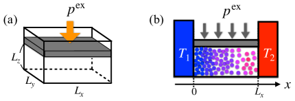
Figure 2: Schematic figures of heat conduction systems at constant pressure. (a) Shape of a container with a movable top plate. (b) Layout of a system with two heat baths.

Throughout this paper, we consider a system of $N$-particles, which are packed in a rectangular container with lengths of side $L_{x}$, $L_{y}$ and $L_{z}$, as shown in Fig. 2(a). We ignore the effect of gravity. $L_{x}$ and $L_{y}$ are fixed throughout this paper. $L_{z}$ is fixed for a constant volume system, or not fixed at constant pressure. We study heat conduction states driven by the temperature difference between two heat baths. As schematically described in Fig.  2(b), a heat bath of temperature $T_{1}$ is attached to the left end ($x=0$) and another heat bath of temperature $T_{2}$ to the right end ($x=L_{x}$). Other four boundaries are thermally insulating. We take $T_{1}\leq T_{2}$ without loss of generality, and $(T_{2}-T_{1})/T_{2}$ is assumed to be so small that the system reaches a unique nonequilibrium steady state in the linear response regime. In such an idealized steady state without any convection, the system is regarded as a one-dimensional system. Local states are homogeneous inside any section perpendicular to the $x$ axis, and therefore, local thermodynamic quantities are considered as functions of $x$.

We introduce a dimensionless parameter $\varepsilon$ that indicates the degree of non-equilibrium as

$$\varepsilon\equiv\frac{\Xi}{T_{\mathrm{m}}},$$ (2.27)

where $\Xi$ is the temperature difference and $T_{\mathrm{m}}$ is the mean temperature of the heat baths, which are defined by

$$\Xi\equiv T_{2}-T_{1},$$ (2.28)

$$T_{\mathrm{m}}\equiv\frac{T_{1}+T_{2}}{2}.$$ (2.29)

When we focus on the linear response regime around an equilibrium state, we ignore the contribution of $O(\varepsilon^{2})$.

2.3 Local equilibrium thermodynamics

For such macroscopic non-equilibrium systems, the hypothesis of local equilibrium thermodynamics works well. That is, local thermodynamic quantities are assumed to satisfy local thermodynamic relations at each space and time Landau-Lifshitz-Fluid ; Groot-Mazur . Now, suppose that the temperature profile $T(x)$, the density profile $\rho(x)$ and the pressure $p(x)$ are determined by experimental observation. Any local thermodynamic quantities, such as $a(x)$ and $\hat{a}(x)$, are expressed as

$$a(x) =a(T(x),\rho(x)),$$ (2.30)

$$\hat{a}(x) =\hat{a}(T(x),p(x)),$$ (2.31)

where functions $a(T,\rho)$ and $\hat{a}(T,p)$ are determined in thermodynamics, as described in the previous subsection. According to (2.19), $a(x)$ may be also written as $a(x)=a(T(x),p(x))$ via $\rho(x)=\rho(T(x),p(x))$. Then, local equilibrium thermodynamics means

$$g(x)=\mu(x)\rho(x),$$ (2.32)

$$s(x)dT(x)+\rho(x)d\mu(x)=dp(x),$$ (2.33)

$$dg(x)=-s(x)dT(x)+\mu(x)d\rho(x)+dp(x),$$ (2.34)

which correspond to the relations (2.20), (2.21) and (2.22), respectively. For the quantities per one particle, we also have

$$\mu(x)=\hat{u}(x)-T(x)\hat{s}(x)+\hat{\phi}(x)p(x),$$ (2.35)

$$d\mu(x)=-\hat{s}(x)dT(x)+\hat{\phi}(x)dp(x),$$ (2.36)

which correspond to the local version of the thermodynamic relations (2.25) and (2.26).

2.4 Global conditions for steady states

For steady state heat conduction, the local pressure $p(x)$ satisfies

$$p(x)=p(x^{\prime})$$ (2.37)

for any $x$ and $x^{\prime}$. Especially, for the system at the constant pressure $p^{\mathrm{ex}}$,

$$p(x)=p^{\mathrm{ex}}$$ (2.38)

holds for any $x$. These equalities for the local pressure may be regarded as global relations because they are not obtained in the local thermodynamics. Furthermore, heat flux $J(x)$ is uniform in $x$ as expressed in the form

$$J(x)=J(x^{\prime})$$ (2.39)

for any $x$ and $x^{\prime}$, which may work as another global relation for the local quantities. In order to connect the heat flux with the local thermodynamic quantities, we assume a heat conduction equation

$$J(x)=-\kappa(T(x),\rho(x))\frac{\partial T(x)}{\partial x},$$ (2.40)

in which $\kappa(T,\rho)$ is heat conductivity as a function of $(T,\rho)$. We assume that there is no temperature gap at the boundaries, i.e.,

$$\lim_{x\rightarrow+0}T(x)=T_{1},\quad\lim_{x\rightarrow L_{x}-0}T(x)=T_{2}.$$ (2.41)

Finally, the conservation of particle number is written as

$$L_{y}L_{z}\int_{0}^{L_{x}}dx~{}\rho(x)=N.$$ (2.42)

These global relations, (2.37), (2.38), (2.39), (2.42), together with the equation of state (2.5), the heat conduction equation (2.40), and the boundary condition (2.41), are sufficient to determine the profiles of the local temperature $T(x)$ and the local density $\rho(x)$ provided that the systems consist of a single phase.

As we will see in §4, there is a case where liquid and gas coexist in the container. For this special situation, the above global relations are not sufficient to determine the local states. This problem will be seriously studied in later sections.

2.5 Global thermodynamic quantities

Since thermodynamic quantities in heat conduction are not uniform in the space, they are basically described as local fields. Nevertheless, from the fact that the local states are governed by the global relations as explained in §2.4, we expect that some properties of the heat conduction systems are explained from a global point of view. Toward the characterization of global properties, we here define global thermodynamic quantities for heat conduction systems.

For extensive variables $A$ originally defined for equilibrium states, we define the following global quantities as an extension to those for heat conduction states:

$${A}=L_{y}L_{z}\int_{0}^{L_{x}}dx~{}a(T(x),p),$$ (2.43)

where we have used the same notation $A$ as that for equilibrium states. When we interpret $A$ as a state function of heat conduction states, we explicitly write $A(T_{1},T_{2},p,N)$ which is in contrast to $A(T,p,N)$ for equilibrium states. For instance, global entropy and global Gibbs free energy are defined as

$${S}=L_{y}L_{z}\int_{0}^{L_{x}}dx~{}s(T(x),p),$$ (2.44)

$${G}=L_{y}L_{z}\int_{0}^{L_{x}}dx~{}g(T(x),p).$$ (2.45)

Here, we investigate the reference state dependence of these global thermodynamic quantities. In equilibrium thermodynamics, entropy density and internal energy density are defined up to an additive constant which depends on the choice of their reference state. Thus, the entropy density $s(x)$ and the internal energy density $u(x)$ possess this property. Concretely, let $\hat{s}_{0}$ and $\hat{u}_{0}$ be the shift of the additive arbitrary constants of entropy and energy per one particle, respectively, for the change of the reference state. We express this transformation by

$$s(x)\rightarrow s(x)+\hat{s}_{0}\rho(x),$$ (2.46)

$$u(x)\rightarrow u(x)+\hat{u}_{0}\rho(x).$$ (2.47)

The shift of other thermodynamic quantities are induced as

$$g(x)\rightarrow g(x)-\hat{s}_{0}\rho(x)T(x)+\hat{u}_{0}\rho(x),$$ (2.48)

$$\mu(x)\rightarrow\mu(x)-\hat{s}_{0}T(x)+\hat{u}_{0}.$$ (2.49)

Note that local thermodynamic relations are invariant under the transformation.

Now, we consider the transformation of the global thermodynamic quantities, which are defined by the spatial integral of the local quantities. It is obvious that

$${S} \rightarrow{S}+\hat{s}_{0}L_{y}L_{z}\int_{0}^{L_{x}}dx~{}~{}\rho(x)={S}+\hat{s}_{0}N,$$ (2.50)

$${U} \rightarrow{U}+\hat{u}_{0}L_{y}L_{z}\int_{0}^{L_{x}}dx~{}~{}\rho(x)={U}+\hat{u}_{0}N,$$ (2.51)

while for the global Gibbs free energy ${G}$, we have

$${G} \rightarrow{G}-\hat{s}_{0}L_{y}L_{z}\int_{0}^{L_{x}}dx~{}~{}\rho(x)T(x)+\hat{u}_{0}L_{y}L_{z}\int_{0}^{L_{x}}dx~{}~{}\rho(x).$$ (2.52)

The $\hat{s}_{0}$ dependence of ${G}$ is far from trivial. Here, we introduce the global temperature ${\tilde{T}}$ such that the transformation is written as

$${G} \rightarrow{G}-\hat{s}_{0}N{\tilde{T}}+\hat{u}_{0}N.$$ (2.53)

Explicitly, ${\tilde{T}}$ is given as

$${\tilde{T}} =\frac{\int_{0}^{L_{x}}dx~{}~{}\rho(x)T(x)}{\int_{0}^{L_{x}}dx~{}~{}\rho(x)},$$ (2.54)

which means that global temperature ${\tilde{T}}$ corresponds to the kinetic temperature averaged over particles. The transformation (2.53) suggests the consistency among ${G}$, ${S}$ and ${\tilde{T}}$. Indeed, we will show the global thermodynamic relations for these quantities. Similarly, we also define the global chemical potential as

$$\tilde{\mu} =\frac{\int_{0}^{L_{x}}dx~{}~{}\rho(x)\mu(x)}{\int_{0}^{L_{x}}dx~{}~{}\rho(x)}.$$ (2.55)

Since $\tilde{\mu}={G}/N$, the global chemical potential corresponds to the Gibbs free energy per one particle.

3 Global thermodynamics for single-phase systems in the linear response regime

In this section, we restrict ourselves to a single phase where the heat conduction system is occupied by either liquid or gas at the constant pressure $p^{\mathrm{ex}}$. When the environmental parameters $T_{1}$, $T_{2}$, and $p^{\mathrm{ex}}$ are fixed, the steady state is uniquely determined from the equation of state (2.5), the heat conduction equation (2.40), and the conservation law (2.42). That is, the values of $(T(x),\rho(x),L_{z})$ are determined by

$$p(T(x),\rho(x))=p^{\mathrm{ex}},$$ (3.1)

$$\frac{\partial}{\partial x}\left[\kappa(T(x),\rho(x))\frac{\partial T(x)}{\partial x}\right]=0,$$ (3.2)

$$L_{z}=\frac{N}{L_{y}\int_{0}^{L_{x}}dx~{}\rho(x)}.$$ (3.3)

Since the local thermodynamic quantities obey equilibrium thermodynamics, the profile $(T(x),\rho(x))$ leads to any local thermodynamic quantities such as $s(x)$ and $\mu(x)$. Then, the global quantities such as ${\tilde{T}}$, $\tilde{\mu}$, and ${S}$ are calculated for the steady state.

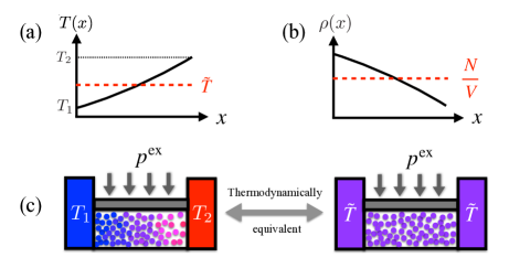
Figure 3: (a) Typical temperature profile $T(x)$. The global temperature ${\tilde{T}}$ is shown in the red dotted line, which satisfies ${\tilde{T}}=(T_{1}+T_{2})/2+O(\varepsilon^{2})$. See (3.54). (b) Typical density profile $\rho(x)$, where its spatial average $N/V$ is displayed by the red dotted line. The global version of the equation of state is given as $p^{\mathrm{ex}}=p({\tilde{T}},N/V)+O(\varepsilon^{2})$ in (3.55). (c) Correspondence of the heat conduction system to the equilibrium system of $({\tilde{T}},p^{\mathrm{ex}},N)$.

Now, we show that the global thermodynamic functions satisfy

$${G}(T_{1},T_{2},p,N)=G({\tilde{T}},p,N)+O(\varepsilon^{2}),$$ (3.4)

$${S}(T_{1},T_{2},p,N)=S({\tilde{T}},p,N)+O(\varepsilon^{2}).$$ (3.5)

This means that the global free energy and entropy, which are functions of $(T_{1},T_{2},p,N)$, are expressed as the equilibrium free energy and the equilibrium entropy when we use the global temperature ${\tilde{T}}$. This result leads to relations among the global quantities as

$$G=U-{\tilde{T}}S+pV+O(\varepsilon^{2}),$$ (3.6)

$$d{G}=-{S}d{\tilde{T}}+Vdp+\tilde{\mu}dN+O(\varepsilon^{2}),$$ (3.7)

which represents the fundamental relation of thermodynamics extended to heat conduction states in the linear response regime. We call such a framework the global thermodynamics for heat conduction systems. These results indicate that, as schematically shown in Fig. 3, the global nature of the heat conduction system is equivalent to that of the equilibrium system. Any global quantity $A$ defined by (2.43) is connected to a corresponding equilibrium quantity $A({\tilde{T}},p,N)$ as

$$A(T_{1},T_{2},p,N)=A({\tilde{T}},p,N)+O(\varepsilon^{2}).$$ (3.8)

3.1 Proof of (3.4) and (3.5)

When the environmental parameters $(T_{1},T_{2},p^{\mathrm{ex}})$ are slightly changed to $(T_{1}+\delta T_{1},T_{2}+\delta T_{2},p^{\mathrm{ex}}+\delta p^{\mathrm{ex}})$, the solution of the equations (3.1), (3.2), and (3.3) is modified slightly. We express the corresponding change as

$$(T(x),\rho(x)) \rightarrow(T(x)+\delta T(x),\rho(x)+\delta\rho(x)),$$ (3.9)

$$L_{z} \rightarrow L_{z}+\delta L_{z},$$ (3.10)

which leads to the change of any local thermodynamic quantity. For instance, the change of the local Gibbs free energy density is given by

$$\delta g(x)=g(T(x)+\delta T(x),p^{\mathrm{ex}}+\delta p^{\mathrm{ex}})-g(T(x),p^{\mathrm{ex}}).$$ (3.11)

The change of the local quantities brings the change of the global quantities as

$${\tilde{T}}\rightarrow{\tilde{T}}+\delta{\tilde{T}},$$ (3.12)

$${G}\rightarrow{G}+\delta{G},$$ (3.13)

where

$$\delta{G} =L_{y}\int_{0}^{L_{x}}dx~{}~{}[(L_{z}+\delta L_{z})g(T(x)+\delta T(x),p^{\mathrm{ex}}+\delta p^{\mathrm{ex}})-L_{z}g(T(x),p^{\mathrm{ex}})],$$

$$=L_{y}\int_{0}^{L_{x}}dx~{}~{}(L_{z}\delta g(x)+g(x)\delta L_{z}).$$ (3.14)

Here, since (2.34) holds for the local densities, the variation of each density satisfies a thermodynamic relation such as

$$\delta g(x)=-s(x)\delta T(x)+\mu(x)\delta\rho(x)+\delta p^{\mathrm{ex}}.$$ (3.15)

By substituting the local relations (2.32) and (3.15) into (3.14), we have

$$\delta{G} =-{S}\delta{\tilde{T}}+V\delta p^{\mathrm{ex}}-\int_{0}^{L_{x}}dx~{}~{}(\hat{s}(x)n(x)\delta\eta(x)-\mu(x)\delta n(x)),$$ (3.16)

where $\hat{s}(x)=s(x)/\rho(x)$ and we have defined

$$\eta(x)\equiv T(x)-{\tilde{T}},\quad n(x)\equiv L_{y}L_{z}\rho(x).$$ (3.17)

Note that $n(x)dx$ is the particle number in $[x,x+dx]$ and that $n(x)$ is estimated as $n(x)=N/L_{x}+O(\varepsilon)$. $\eta(x)$ is the deviation of the local temperature $T(x)$ from the global temperature ${\tilde{T}}$, and is estimated as $\eta(x)=O(\varepsilon)$.

Since any local thermodynamic quantity $a(x)$ is regarded as $a(T(x),p^{\mathrm{ex}})=a({\tilde{T}}+\eta(x),p^{\mathrm{ex}})$, we may estimate $a(x)=a({\tilde{T}},p^{\mathrm{ex}})+O(\varepsilon)$. Then, the integrant in (3.16) is estimated as

$$\hat{s}(x)n(x)\delta\eta(x)-\mu(x)\delta n(x) =\hat{s}(x)\delta(n(x)\eta(x))-(\hat{s}(x)\eta(x)+\mu(x))\delta n(x)$$

$$=\hat{s}({\tilde{T}},p)\delta(n(x)\eta(x))-\mu({\tilde{T}},p^{\mathrm{ex}})\delta n(x)+O(\varepsilon^{2}),$$ (3.18)

where $\delta n(x)=O(\varepsilon)$ for $N$ and $L_{x}$ fixed. We find that

$$\int_{0}^{L_{x}}dx~{}~{}n(x)\eta(x)=0$$ (3.19)

holds from (2.54). Obviously, the conservation of the particle number leads to

$$\int_{0}^{L_{x}}dx~{}~{}\delta n(x)=0.$$ (3.20)

Thus, the integral in (3.16) is estimated as

$$\int_{0}^{L_{x}}dx~{}~{}(\hat{s}(x)n(x)\delta\eta(x)-\mu(x)\delta n(x))=O(\varepsilon^{2}),$$ (3.21)

and then (3.16) becomes

$$\delta{G} =-{S}\delta{\tilde{T}}+V\delta p^{\mathrm{ex}}+O(\varepsilon^{2}).$$ (3.22)

We emphasize that the definition of ${\tilde{T}}$ in (2.54) is essential for this relation.

Here, let us recall that the value of ${G}$ is determined for a given $(T_{1},T_{2},p^{\mathrm{ex}},N)$. Since there is one-to-one correspondence between $({\tilde{T}},\varepsilon)$ and $(T_{1},T_{2})$, ${G}$ is given as a function of $({\tilde{T}},p^{\mathrm{ex}},N,\varepsilon)$. The relation (3.22) implies that ${G}$ is independent of $\varepsilon$ in the linear response regime, and thus given as a function of $({\tilde{T}},p^{\mathrm{ex}},N)$. Therefore, we conclude (3.4). Next, we show (3.5). From the relation (3.22), the left-hand side of (3.5) is expressed as

$${S}(T_{1},T_{2},p^{\mathrm{ex}},N)=-\left(\frac{\partial{G}}{\partial{\tilde{T}}}\right)_{p^{\mathrm{ex}},N}+O(\varepsilon^{2}),$$ (3.23)

while the equilibrium fundamental relation results in

$$S({\tilde{T}},p^{\mathrm{ex}},N)=-\left(\frac{\partial{G}}{\partial{\tilde{T}}}\right)_{p^{\mathrm{ex}},N}.$$ (3.24)

Combining these two equalities, we obtain (3.5).

The definition (2.55) for the global chemical potential $\tilde{\mu}$ indicates $\tilde{\mu}=G/N$. Then, (3.4) leads to

$$\tilde{\mu}(T_{1},T_{2},p)=\mu({\tilde{T}},p)+O(\varepsilon^{2}).$$ (3.25)

We thus find

$$d\tilde{\mu} =-\hat{s}d{\tilde{T}}+\hat{\phi}dp+O(\varepsilon^{2}),$$ (3.26)

where

$$\hat{s}\equiv\frac{S}{N},\quad\hat{\phi}\equiv\frac{V}{N},$$ (3.27)

are entropy per one particle and specific volume of the heat conduction system.

3.2 Various global thermodynamic functions

From a local relation $f(x)=g(x)-p$, we have

$${F}={G}-pV.$$ (3.28)

By using (3.4), we obtain

$${F}(T_{1},T_{2},V,N)=F({\tilde{T}},V,N)+O(\varepsilon^{2}).$$ (3.29)

We thus have the fundamental relation for ${F}$

$$d{F}=-{S}d{\tilde{T}}-pdV+\tilde{\mu}dN+O(\varepsilon^{2})$$ (3.30)

in the linear response regime.

Next, we consider the global internal energy ${U}$ and the global enthalpy ${H}$. From local thermodynamic relations $u(x)=f(x)+T(x)s(x)$ and $h(x)=g(x)+T(x)s(x)$, we write

$${U}={F}+{\tilde{T}}{S}+\int_{0}^{L_{x}}dx~{}~{}\hat{s}(x)\eta(x)n(x),$$ (3.31)

$${H}={G}+{\tilde{T}}{S}+\int_{0}^{L_{x}}dx~{}~{}\hat{s}(x)\eta(x)n(x).$$ (3.32)

Remembering that $\eta(x)=O(\varepsilon)$, the integral is estimated as

$$\int_{0}^{L_{x}}dx~{}~{}\hat{s}(x)\eta(x)n(x) =\hat{s}({\tilde{T}},P)\int_{0}^{L_{x}}dx~{}~{}n(x)\eta(x)+O(\varepsilon^{2})$$

$$=O(\varepsilon^{2}),$$ (3.33)

where we have used (3.19). Thus, we obtain

$${U} ={F}+{\tilde{T}}{S}+O(\varepsilon^{2})$$ (3.34)

$${H} ={G}+{\tilde{T}}{S}+O(\varepsilon^{2})$$ (3.35)

Substituting (3.4),(3.5),(3.29) into (3.34) and (3.35), we have

$${U}(T_{1},T_{2},V,N) =U({S},V,N)+O(\varepsilon^{2}),$$ (3.36)

$${H}(T_{1},T_{2},p,N) =H({S},p,N)+O(\varepsilon^{2}).$$ (3.37)

3.3 Clausius equality

Since the thermodynamic relations are extended with keeping the same forms as those in equilibrium thermodynamics, we may define quasi-static heat $d^{\prime}Q$ in an infinitely small quasi-static process $(T_{1},T_{2},p^{\mathrm{ex}})\to(T_{1}+\delta T_{1},T_{2}+\delta T_{2},p^{\mathrm{ex}}+\delta p^{\mathrm{ex}})$ as

$${d^{\prime}Q}={\tilde{T}}\delta S.$$ (3.38)

This $d^{\prime}Q$ corresponds to the absorbed heat by the system, which is the sum of the heat from the left and right heat baths during the infinitesimal change. There, by summing the two heats, the net heat flow is canceled. If the heat absorbed from the right heat bath is exactly the same as the heat released from the left heat bath at every moment during the process, the net heat vanishes for the heat conduction. Such systems are thought to be adiabatic in the sense of global thermodynamics, and

$$dS=0$$ (3.39)

in such a quasi-static adiabatic process in the linear response regime.

Then, constant-pressure heat capacity is defined as

$$C_{p}\equiv\left(\frac{d^{\prime}Q}{d{\tilde{T}}}\right)_{p}.$$ (3.40)

Applying the thermodynamic relation, we obtain

$$C_{p}(T_{1},T_{2},p,N) =\left(\frac{\partial H}{\partial{\tilde{T}}}\right)_{p}+O(\varepsilon^{2})$$ (3.41)

$$={\tilde{T}}\left(\frac{\partial S}{\partial{\tilde{T}}}\right)_{p}+O(\varepsilon^{2}).$$ (3.42)

Note that $C_{p}$ is defined as the response to the change of the global temperature ${\tilde{T}}$. By changing the temperatures of heat baths, ${\tilde{T}}$ may change in accordance with absorbing heat corresponding to $C_{p}\delta{\tilde{T}}$.

3.4 Correspondence of global thermodynamic quantities to equilibrium quantities

In the previous subsections, we have obtained thermodynamic relations in the linear response regime and found that they are equivalent to the equilibrium ones. The key concept for extending thermodynamics is the global temperature ${\tilde{T}}$ and the global chemical potential $\tilde{\mu}$, by which the heat conduction system of $({\tilde{T}},\tilde{\mu})$ is mapped to the equilibrium system of $({\tilde{T}},\tilde{\mu})$. The connection between the two thermodynamic frameworks becomes clearer in the argument below by considering the estimation method of global thermodynamic quantities.

In a single phase system, local temperature $T(x)$ is a continuous monotonic function of $x$. Any extensive quantity $A$, which is defined as a spatial integral of local density $a(x)$, can be transformed into an integral over temperature:

$${A} =L_{y}L_{z}\int_{0}^{L_{x}}dx~{}~{}a(T(x),p)$$

$$=\frac{V}{T_{2}-T_{1}}\int_{T_{1}}^{T_{2}}dT~{}\psi(T,p),$$ (3.43)

where

$$\psi(T,p)\equiv\frac{a(T,p)}{{\cal J}(T)},$$ (3.44)

$${\cal J}(T)\equiv\frac{L_{x}}{T_{2}-T_{1}}\left(\frac{dx(T)}{dT}\right)^{-1}.$$ (3.45)

We expand $\psi(T,P)$ around $T=T_{\mathrm{m}}$ in the form

$$\psi(T,p)=\psi(T_{\mathrm{m}},p)+\left.\left(\frac{\partial\psi}{\partial T}\right)_{p}\right|_{T_{\mathrm{m}}}(T-T_{\mathrm{m}})+O(\varepsilon^{2}).$$ (3.46)

The second term is canceled when the integral (3.43) is performed. We thus have an estimation

$${A} =V\psi(T_{\mathrm{m}},p)+O(\varepsilon^{2})$$

$$=V\frac{a(T_{\mathrm{m}},p)}{{\cal J}(T_{\mathrm{m}})}+O(\varepsilon^{2}).$$ (3.47)

For $A=V$, we have $a(x)=1$ for all $x$. By combining this with (3.47), we find

$${{\cal J}(T_{\mathrm{m}})}=1+O(\varepsilon^{2}).$$ (3.48)

We then have arrived at a universal estimation of the global quantity $A$ as

$${A}(T_{1},T_{2},p,N)=A(T_{\mathrm{m}},p,N)+O(\varepsilon^{2}),$$ (3.49)

where $A(T_{\mathrm{m}},p,N)=Va(T_{\mathrm{m}},p)$. The result (3.49) directly connects the global quantity in the heat conduction state to the corresponding equilibrium quantity at $T_{\mathrm{m}}$.

We may apply the similar method to the global temperature. The global temperature is also written as

$${\tilde{T}} =\frac{L_{y}L_{z}}{N}\int_{0}^{L_{x}}dx~{}~{}\rho(x)T(x)$$ (3.50)

$$=\frac{V}{N}\rho(T_{\mathrm{m}},p)T_{\mathrm{m}}+O(\varepsilon^{2}),$$ (3.51)

in which

$$N =L_{y}L_{Z}\int_{0}^{L_{x}}dx~{}~{}\rho(x)$$ (3.52)

$$=V\rho(T_{\mathrm{m}},p).$$ (3.53)

By substituting it into (3.51), we obtain

$${\tilde{T}}=T_{\mathrm{m}}+O(\varepsilon^{2}).$$ (3.54)

Thus, in the linear response regime, the global temperature ${\tilde{T}}$ in the heat conduction system is equal to the mean temperature $T_{\mathrm{m}}$ of the heat baths. The relation (3.49), together with (3.54), concludes (3.8). We also note that (3.53), which is rewritten as $\rho=\rho({\tilde{T}},p)+O(\varepsilon^{2})$ with $\rho=N/V$, corresponds to the global version of the equation of state

$$p=p({\tilde{T}},N/V)+O(\varepsilon^{2}).$$ (3.55)

We here remark that the relation ${\tilde{T}}=T_{\mathrm{m}}$ in the linear response regime is a specific feature of systems in a rectangular container. We will show in §10.2 that the global temperature deviates from the mean temperature when the shape of the container is not a rectangle, whereas the relation (3.8) still holds.

4 Liquid-gas coexistence in heat conduction

From now on, we study liquid-gas coexistence in heat conduction. In §4.1, we review thermodynamics under equilibrium conditions while paying attention to the description of metastable states. In §4.2, we describe heat conduction states based on local equilibrium thermodynamics. We explain how the temperature profile and the density profile are determined for a given position of the liquid-gas interface. In §4.3, we present global thermodynamic quantities as a function of the interface position. In §4.4, we address the main problem of thermodynamics for the heat conduction systems with the liquid-gas coexistence. Hereafter, superscripts $\mathrm{L}$ and $\mathrm{G}$ are attached to quantities related to liquid and gas, respectively.

4.1 Thermodynamics under equilibrium conditions

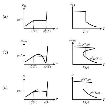
Figure 4: Three kinds of equation of state: (a) Equilibrium pressure, (b) van der Waals pressure, and (c) experimentally measured pressure. $p_{\rm s}(T)$ is saturated pressure in liquid-gas transition for a given $T$ below the critical temperature. $T_{\mathrm{c}}(p)$ is transition temperature for a given $p$. $\rho^{\mathrm{L/G}}_{\rm s}$ denotes saturated density, which is defined by $\rho^{\mathrm{L/G}}_{\rm s}=\rho^{\mathrm{L/G}}(T,p_{\rm s}(T))$.

We first consider equilibrium thermodynamics. For a given $(T,\rho)$, the pressure $p$ is uniquely determined even when phase coexistence is observed. This equation of state is expressed as

$$p=p_{\rm eq}(T,\rho)$$ (4.1)

so as to emphasize that the pressure is the equilibrium value. See Fig. 4(a). A remarkable fact is that there is a plateau region $[\rho^{\mathrm{G}}_{\rm s}(T),\rho^{\mathrm{L}}_{\rm s}(T)]$ for a given temperature $T$ below the critical temperature. From this equation of state, we find that the density $\rho$ exhibits the discontinuous change at $T=T_{\mathrm{c}}(p)$ when the temperature is changed with the pressure $p$ fixed, as shown in Fig. 4(a). That is, the whole system is occupied by liquid when $T<T_{\mathrm{c}}(p)$, while by gas when $T>T_{\mathrm{c}}(p)$.

In experiments, metastable states, which also may be called quasi-equilibrium states, are often observed. The most typical approach to the description of such meta-stable states is to employ the van der Waals equation of state:

$$p= p_{\mathrm{vdW}}(T,\rho)$$

$$= \frac{\rho k_{\rm B}T}{1-\rho b}-a\rho^{2},$$ (4.2)

where $k_{\mathrm{B}}$ is the Boltzmann constant. The constants $a$ and $b$ are van der Waals parameters. When $T$ is fixed as that below the critical temperature, the equation of state contains the unstable states $(\partial\rho/\partial p)_{T}<0$. See Fig. 4(b). Following the standard procedure of the Maxwell construction, we obtain the equilibrium equation of state from (4.2). Here, we extract the two stable branches satisfying $(\partial\rho/\partial p)_{T}\geq 0$ from the curve defined by (4.2), each of which is connected to the equilibrium liquid phase or to the equilibrium gas phase. By solving (4.2) in $\rho$ for each region, we obtain

$$\rho=\rho_{\mathrm{vdW}}^{\mathrm{L}}(T,p)\quad\mbox{for liquid},$$ (4.3)

$$\rho=\rho_{\mathrm{vdW}}^{\mathrm{G}}(T,p)\quad\mbox{for gas}.$$ (4.4)

When $\rho_{\mathrm{vdW}}^{\mathrm{G}}(T,p)>\rho^{\mathrm{G}}_{\rm s}(T)$, the spatially homogeneous phase of $(T,p)$ corresponds to a meta-stable gas. Similarly, when $\rho_{\mathrm{vdW}}^{\mathrm{L}}(T,p)<\rho^{\mathrm{L}}_{\rm s}(T)$, the homogeneous phase of $(T,p)$ corresponds to a meta-stable liquid. By plotting $\rho$ as a function of $T$ with $p$ fixed as shown in Fig. 4(b), one finds that the meta-stable gas and the meta-stable liquid are super-cooled gas and super-heated liquid, respectively.

More generally, without using the van der Waals equation of state, we may obtain

$$\rho=\rho^{\mathrm{L}}(T,P)\quad\mbox{for liquid},$$ (4.5)

$$\rho=\rho^{\mathrm{G}}(T,P)\quad\mbox{for gas},$$ (4.6)

by experimental measurements. See Fig. 4(c). Below we assume (4.5) and (4.6), whereas one may interpret them as (4.3) and (4.4). We then define densities for the liquid phase and the gas phase as

$$a^{\mathrm{L}}(T,p)\equiv a(T,\rho^{\mathrm{L}}(T,p)),\qquad a^{\mathrm{G}}(T,p)\equiv a(T,\rho^{\mathrm{G}}(T,p)),$$ (4.7)

and define quantities per one particle for the liquid phase and the gas phase as

$$\hat{a}^{\mathrm{L}}(T,p)\equiv\frac{a(T,\rho^{\mathrm{L}}(T,p))}{\rho^{\mathrm{L}}(T,p)},\qquad\hat{a}^{\mathrm{G}}(T,p)\equiv\frac{a(T,\rho^{\mathrm{G}}(T,p))}{\rho^{\mathrm{G}}(T,p)}.$$ (4.8)

4.2 Heat conduction states

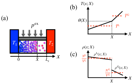
Figure 5: (a) Schematic figure of the liquid-gas coexistence with the interface position $X$. (b) Temperature profile $T(x;X)$ is continuous but not smooth at $x=X$, where the interface temperature satisfies $\theta(X)=T(X;X)$. The global temperatures in the liquid region and the gas region, ${\tilde{T}}^{\mathrm{L}}$ and ${\tilde{T}}^{\mathrm{G}}$, are displayed by the red dotted lines, respectively. See (4.27). (c) Density profile $\rho(x;X)$ shows a jump at $x=X$, where $\rho^{\mathrm{L}}(x;X)\equiv\rho^{\mathrm{L}}(T(x;X),p)$ and $\rho^{\mathrm{G}}(x;X)\equiv\rho^{\mathrm{L}}(T(x;X),p)$. Since global thermodynamics holds for each region, the equation of state (3.55) leads to $p^{\mathrm{ex}}=p({\tilde{T}}^{\mathrm{L}},N^{\mathrm{L}}/V^{\mathrm{L}})+O(\varepsilon^{2})=p({\tilde{T}}^{\mathrm{G}},N^{\mathrm{G}}/V^{\mathrm{G}})+O(\varepsilon^{2})$.

When $T_{1}<T_{\mathrm{c}}(p^{\mathrm{ex}})<T_{2}$, we may observe liquid-gas coexistence at the constant pressure $p^{\mathrm{ex}}$, which is in contrast with equilibrium cases. Concretely, the liquid occupies a lower temperature region, while the gas does a higher temperature region, as shown in Fig. 5(a). We assume that both the interface width and the temperature gap at the interface are negligible. See Fig. 5(b). Then, let $X$ denote the position of the interface. Although the value of $X$ should be uniquely determined under given conditions, we shall formally treat $X$ as if it were an independent variable in what follows. The density profile for a given $X$ is then expressed as

$$\rho(x;X)=\left\{\begin{array}[]{lll}\rho^{\mathrm{L}}(T(x;X),p^{\mathrm{ex}})&~{}~{}\mbox{for}&~{}~{}0\leq x<X,\\ \rho^{\mathrm{G}}(T(x;X),p^{\mathrm{ex}})&~{}~{}\mbox{for}&~{}~{}X<x\leq L_{x}.\end{array}\right.$$ (4.11)

See Fig. 5(b). The temperature profile $T(x;X)$ is determined by the heat conduction equation

$$J(X)=\left\{\begin{array}[]{lll}-\kappa^{\mathrm{L}}(T(x;X),p^{\mathrm{ex}}){\displaystyle\frac{\partial T(x;X)}{\partial x}}&~{}~{}\mbox{for}&~{}~{}0<x<X,\\ -\kappa^{\mathrm{G}}(T(x;X),p^{\mathrm{ex}}){\displaystyle\frac{\partial T(x;X)}{\partial x}}&~{}~{}\mbox{for}&~{}~{}X<x<L_{x},\end{array}\right.$$ (4.14)

where $J(X)$ is the steady heat current which is constant in $x$ due to the conservation of energy. The boundary conditions for the equation (4.14) are

$$\lim_{x\rightarrow+0}T(x;X)=T_{1},\quad\lim_{x\rightarrow L_{x}-0}T(x;X)=T_{2}.$$ (4.15)

Concretely, $T(x;X)$ is obtained as follows. We first express the interface temperature as $\theta(X)$:

$$\theta(X)=T(X;X).$$ (4.16)

By setting

$$\kappa^{\mathrm{L/G}}_{\mathrm{c}}\equiv\kappa^{\mathrm{L/G}}(T_{\mathrm{c}}(p^{\mathrm{ex}}),p^{\mathrm{ex}}),$$ (4.17)

we find that the local heat conductivity is estimated as

$$\kappa^{\mathrm{L/G}}(T(x),p^{\mathrm{ex}})=\kappa^{\mathrm{L/G}}_{\mathrm{c}}+O(\varepsilon).$$ (4.18)

Then, (4.14) leads to

$$J(X)=-\kappa^{\mathrm{L}}_{\mathrm{c}}\frac{\theta(X)-T_{1}}{X}+O(\varepsilon^{2})=-\kappa^{\mathrm{G}}_{\mathrm{c}}\frac{T_{2}-\theta(X)}{L_{x}-X}+O(\varepsilon^{2}).$$ (4.19)

Solving the second equality of (4.19) in $\theta(X)$, we obtain

$$\theta(X)=T_{\mathrm{m}}+\frac{\Xi}{2}\left(\frac{X}{\kappa^{\mathrm{L}}_{\mathrm{c}}}-\frac{L_{x}-X}{\kappa^{\mathrm{G}}_{\mathrm{c}}}\right)\left(\frac{X}{\kappa^{\mathrm{L}}_{\mathrm{c}}}+\frac{L_{x}-X}{\kappa^{\mathrm{G}}_{\mathrm{c}}}\right)^{-1}+O(\varepsilon^{2}).$$ (4.20)

Defining the scaled position $\zeta$ of the interface and an effective heat conductivity $\kappa_{\rm eff}(\zeta)$ as

$$\zeta\equiv\frac{X}{L_{x}},\qquad\kappa_{\rm eff}(\zeta)\equiv\left(\frac{\zeta}{\kappa^{\mathrm{L}}_{\mathrm{c}}}+\frac{1-\zeta}{\kappa^{\mathrm{G}}_{\mathrm{c}}}\right)^{-1},$$ (4.21)

we have

$$J(X)=-\kappa_{\rm eff}(\zeta)\frac{\Xi}{L_{x}}+O(\varepsilon^{2}),$$ (4.22)

which is obtained by substituting (4.20) into (4.19).

By using $\theta(X)$ given by (4.20), the temperature profile is written as

$$T(x;X)=\left\{\begin{array}[]{ll}T_{1}+{\displaystyle\frac{x}{X}}(\theta(X)-T_{1})+O(\varepsilon^{2})&\mbox{for}~{}~{}0<x<X,\\ T_{2}-{\displaystyle\frac{L_{x}-x}{L_{x}-X}}(\theta(X)-T_{2})+O(\varepsilon^{2})&\mbox{for}~{}~{}X<x<L_{x}.\end{array}\right.$$ (4.25)

Substituting this profile into the equation of state (4.11), we have $\rho(x;X)$ explicitly as exemplified in Fig. 5(c).

4.3 Global quantities as a function of $X$

The system with the phase coexistence is interpreted as a composite system of a liquid region and a gas region. For each subsystem, we may define global thermodynamic quantities introduced in §3. In this section, we express global thermodynamic quantities as a function of $X$.

First, the global temperatures in the liquid region and in the gas region are defined by

$${\tilde{T}}^{\mathrm{L}}=\frac{\int_{0}^{X}dx~{}\rho(x)T(x)}{\int_{0}^{X}dx~{}\rho(x)},\qquad{\tilde{T}}^{\mathrm{G}}=\frac{\int_{X}^{L_{x}}dx~{}\rho(x)T(x)}{\int_{X}^{L_{x}}dx~{}\rho(x)}.$$ (4.26)

In each region, the temperature profile and the density profile are smooth. We describe each subsystem as a single phase system discussed in §3. The boundary temperatures of the liquid are $T_{1}$ and $\theta$, and those of the gas are $\theta$ and $T_{2}$. Thus, applying the trapezoidal rule explained in §3.4 to (4.26), the global temperature in each region is expressed as

$${\tilde{T}}^{\mathrm{L}}(X)=\frac{T_{1}+\theta(X)}{2}+O(\varepsilon^{2}),\qquad{\tilde{T}}^{\mathrm{G}}(X)=\frac{\theta(X)+T_{2}}{2}+O(\varepsilon^{2}),$$ (4.27)

where we explicitly write the dependence on the interface position $X$. See Fig. 5(b).

Next, the volume of the whole system $V(X)$ is expressed as

$$V(X) =L_{x}\frac{N}{\int_{0}^{L_{x}}dx~{}\rho(x;X)}$$

$$=\frac{N}{\zeta\rho^{\mathrm{L}}({\tilde{T}}^{\mathrm{L}}(X),p^{\mathrm{ex}})+(1-\zeta)\rho^{\mathrm{G}}({\tilde{T}}^{\mathrm{G}}(X),p^{\mathrm{ex}})}+O(\varepsilon^{2}),$$ (4.28)

and thus the volume of the liquid region $V^{\mathrm{L}}(X)$ and the volume of the gas region $V^{\mathrm{G}}(X)$ are written as

$$V^{\mathrm{L}}(X)=\zeta V(X),\qquad V^{\mathrm{G}}(X)=(1-\zeta)V(X).$$ (4.29)

Then, the particle number in the liquid region, $N^{\mathrm{L}}$, is obtained as

$$N^{\mathrm{L}}(X) =V^{\mathrm{L}}(X)\rho^{\mathrm{L}}({\tilde{T}}^{\mathrm{L}}(X),p^{\mathrm{ex}})$$

$$=N\frac{\zeta\rho^{\mathrm{L}}({\tilde{T}}^{\mathrm{L}}(X),p^{\mathrm{ex}})}{\zeta\rho^{\mathrm{L}}({\tilde{T}}^{\mathrm{L}}(X),p^{\mathrm{ex}})+(1-\zeta)\rho^{\mathrm{G}}({\tilde{T}}^{\mathrm{G}}(X),p^{\mathrm{ex}})}+O(\varepsilon^{2}).$$ (4.30)

The particle number in the gas region, $N^{\mathrm{G}}$, is immediately given by

$$N^{\mathrm{G}}(X)=N-N^{\mathrm{L}}(X).$$ (4.31)

By using ${\tilde{T}}^{\mathrm{L}}(X)$, ${\tilde{T}}^{\mathrm{G}}(X)$, and $N^{\mathrm{L}}(X)$, we can express all global thermodynamic quantities in the liquid region and the gas region. Explicitly, the extensive quantities are defined as

$${A}^{\mathrm{L}}\equiv L_{y}L_{z}\int_{0}^{X}dx~{}a^{\mathrm{L}}(T(x),p^{\mathrm{ex}}),$$ (4.32)

$${A}^{\mathrm{G}}\equiv L_{y}L_{z}\int_{X}^{L_{x}}dx~{}a^{\mathrm{G}}(T(x),p^{\mathrm{ex}}).$$ (4.33)

Noting (3.8) in §3 with (2.24), we conclude that the global extensive quantities are written as

$${A}^{\mathrm{L}}(X)=N^{\mathrm{L}}(X)\hat{a}^{\mathrm{L}}({\tilde{T}}^{\mathrm{L}}(X),p^{\mathrm{ex}})+O(\varepsilon^{2}),$$ (4.34)

$${A}^{\mathrm{G}}(X)=N^{\mathrm{G}}(X)\hat{a}^{\mathrm{G}}({\tilde{T}}^{\mathrm{G}}(X),p^{\mathrm{ex}})+O(\varepsilon^{2}).$$ (4.35)

Finally, we define the global temperature for the whole system by the formula (2.54), which is rewritten as

$${\tilde{T}}(X)=\frac{N^{\mathrm{L}}(X)}{N}{\tilde{T}}^{\mathrm{L}}(X)+\frac{N^{\mathrm{G}}(X)}{N}{\tilde{T}}^{\mathrm{G}}(X).$$ (4.36)

4.4 Problem

We have shown that all thermodynamic quantities are determined for a given position $X$ of the liquid-gas interface. Since the liquid-gas interface in heat conduction may be at rest at constant pressure, the position $X$ is uniquely determined for $(T_{1},T_{2},p^{\mathrm{ex}})$.

For equilibrium cases, the phase coexistence is observed in a container with $V$ and $T$ fixed. When we start with the van der Waals equation of state, we can determine the interface position of the two phases by the Maxwell construction, which is equivalent to the continuity of the chemical potential at the interface. Recalling this theory, one may impose the continuity of the local chemical potential $\mu(x)$ at the interface even in heat conduction Bedeauz86 . Since $\mu^{\mathrm{L}}(T_{\mathrm{c}}(p))=\mu^{\mathrm{G}}(T_{\mathrm{c}}(p))$, it leads to $\theta=T_{\mathrm{c}}(p^{\mathrm{ex}})$. That is, under this assumption, the interface temperature is equal to the equilibrium transition temperature.

Here, the important observation is that there is no justification of this condition for heat conduction systems. To our best knowledge, there are no experimental measurements on this issue, no numerical simulations of sufficiently large systems, and no reliable theory for supporting this condition. To be more precise, although the continuity of the chemical potential was reported in numerical simulations Bedeaux00 ; Ogushi , the system size was too small to draw a definite conclusion. One may also recall from a viewpoint of non-equilibrium statistical mechanics that the local equilibrium distribution may be the leading contribution Bertini-rev . However, it should be noted that in the standard approach, fluctuations are described as those around the most probable profile, while the most probable profile itself is undetermined in the current problem. Therefore, the previous studies starting with the local equilibrium distribution do not result in the continuity of the chemical potential without imposing an additional assumption.

Furthermore, as another theoretical approach, one may study the stationary solution of the deterministic equation for the generalized Navier-Stokes equation with the interface thermodynamics Bedeaux03 ; Onuki . We can estimate the discontinuous jump of the chemical potential at the interface as $\varepsilon(w/L_{x})T_{\mathrm{c}}$ based on reasonable assumptions SNIN , where $w$ represents the interface width. This result indicates the validity of the continuity of the chemical potential at the interface, because we may assume $w/L_{x}\ll 1$. However, as carefully argued in the paper SNIN , fluctuation effects should be taken into account for the generalized Navier-Stokes equation, so as to quantitatively describe the thermodynamic behavior.

Now, based on these facts, we reconsider the continuity of the chemical potential at the liquid-gas interface within the framework of equilibrium thermodynamics. We then find that the continuity is equivalent to the thermodynamic variational principle. If the principle were applied to a local sub-system including the interface, the continuity of the chemical potential would be concluded. However, the constraint of a variational principle is generally applied to a whole system but not to the local subsystem, and therefore no variational principle is expected for the local subsystem near the interface. Thus we cannot justify the continuity of the chemical potential. This suggests an alternative approach to determine the interface position $X$. Namely, we formulate a variational principle for the whole heat conduction system as a natural extension of the equilibrium variational principle.

5 Variational principle for determining the liquid-gas interface position

All our discussion on global thermodynamics so far has been firmly based on well-established local equilibrium thermodynamics. Now, we formulate the variational principle for determining the interface position $X$ and solve the variational problem. In §5.1, we start with the simplest example of the variational principle for equilibrium systems and naturally extend it to that for heat conduction systems. In §5.2 we derive the steady-state value by solving the minimization of the variational function. The solution is then reformulated as the temperature relation in §5.3. By using these results, in §5.4, we express the global quantities in terms of $(\tilde{T},p^{\mathrm{ex}},\Xi)$.

5.1 Variational principle

5.1.1 Equilibrium systems

We start with an example of the variational principle for equilibrium systems. We consider a system at the constant pressure $p^{\mathrm{ex}}$ in contact with a heat bath of the temperature $T$. Since the volume $V$ of the system is not fixed, we determine $V$ for a given $(T,p^{\mathrm{ex}})$. When the equation of state is assumed, it is determined from the pressure balance equation

$$p^{\mathrm{ex}}=p(T,V/N).$$ (5.1)

We attempt to derive this condition from a variational principle. We take a variational function ${\cal G}({\cal V};T,p^{\mathrm{ex}},N)$ as

$${\cal G}({\cal V};T,p^{\mathrm{ex}},N)=F(T,{\cal V},N)+p^{\mathrm{ex}}{\cal V}.$$ (5.2)

This corresponds to the Helmholtz free energy minimum principle for the composite system of the system and the volume reservoir whose Helmholtz free energy is $p^{\mathrm{ex}}V+{\rm const}$. We then find that the minimization of ${\cal G}$ with respect to $\cal V$ for $(T,p^{\mathrm{ex}},N)$ fixed leads to (5.1). The volume in the equilibrium state satisfies

$$V=\operatorname*{arg\,min}_{\cal V}{\cal G}({\cal V};T,p^{\mathrm{ex}},N),$$ (5.3)

with which the Gibbs free energy is determined as

$$G(T,p^{\mathrm{ex}},N) =\min_{\cal V}{\cal G}({\cal V};T,p^{\mathrm{ex}},N)$$ (5.4)

$$=F(T,V,N)+p^{\mathrm{ex}}V.$$ (5.5)

It should be noted that this principle may be applied to the case that $F(T,V,N)$ is given by the van der Waals free energy:

$$F(T,V,N)=\frac{3}{2}Nk_{\rm B}T-a\frac{N}{V}-Nk_{\rm B}T\log\frac{T^{3/2}(V-Nb)}{N^{5/2}}.$$ (5.6)

The variational principle for this case is equivalent to the Maxwell construction.

5.1.2 Extension to heat conduction systems

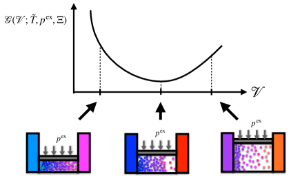
Figure 6: The variational function ${\cal G}({\cal V})$ with $({\tilde{T}},p^{\mathrm{ex}},\Xi)$ fixed for the heat conduction system. $T_{1}$ and $T_{2}$ may depend on ${\cal V}$ in order to fix $\tilde{T}$ and $\Xi$. The configuration corresponding to the minimum of $\cal G$, the mid of the three configurations in the bottom of the figure, is selected as the steady state for $(\tilde{T},p^{\mathrm{ex}},\Xi)$.

We study heat conduction systems at the constant pressure $p^{\mathrm{ex}}$. First, we focus on single-phase systems studied in §3. From the equivalence between a heat conduction system and the corresponding equilibrium system, the volume $V$ of this system is determined by the minimization of

$${\cal G}({\cal V};{\tilde{T}},p^{\mathrm{ex}},N)={F}({\tilde{T}},{\cal V},N)+p^{\mathrm{ex}}{\cal V},$$ (5.7)

where ${\tilde{T}}$ is the global temperature of the system. Since ${F}=F({\tilde{T}},V,N)+O(\varepsilon^{2})$, we rewrite (5.7) as

$${\cal G}({\cal V};{\tilde{T}},p^{\mathrm{ex}},N)=L_{y}L_{z}\int_{0}^{L_{x}}dx[f(T(x),\rho(x))+p^{\mathrm{ex}}]+O(\varepsilon^{2}),$$ (5.8)

where $L_{z}={\cal V}/(L_{x}L_{y})$ depends on $\cal V$ and ${\tilde{T}}$ should be fixed in the variation of $\cal V$. Then, the variational principle (5.3) holds for single-phase systems. Since this formula relies on the equivalence to the equilibrium system, we do not need to fix the degree of nonequilibrium in the variation.

Next, we consider a system with a liquid-gas interface. In this case, $V$ is not determined when we use the equation of state for each region, because the interface position $X$ is not determined yet as described in the previous section. We then assume that the minimization of (5.8) is also valid for such cases, where $\Xi=T_{2}-T_{1}$ is also fixed in the variation $V$. The last property is necessary to determine the value $V$ uniquely. That is, we define a variational function

$${\cal G}({\cal V};{\tilde{T}},p^{\mathrm{ex}},\Xi,N)=L_{y}L_{z}\int_{0}^{L_{x}}dx[f(T(x),\rho(x))+p^{\mathrm{ex}}]$$ (5.9)

and propose that the volume of the system $V$ is determined as

$$\left.\frac{\partial{\cal G}({\cal V};{\tilde{T}},p^{\mathrm{ex}},\Xi,N)}{\partial{\cal V}}\right|_{{\cal V}=V}=0,$$ (5.10)

with

$$\left.\frac{\partial^{2}{\cal G}({\cal V};{\tilde{T}},p^{\mathrm{ex}},\Xi,N)}{\partial{\cal V}^{2}}\right|_{{\cal V}=V}>0.$$ (5.11)

This variational principle was first proposed in Ref. NS .

5.1.3 Remarks

Since the volume $V$ is uniquely determined by the interface position $X$ with $({\tilde{T}},p^{\mathrm{ex}},\Xi,N)$ fixed, as explicitly shown in (4.28), the variational principle (5.10) with (5.11) is expressed as

$$\left.\frac{\partial{\cal G}({\cal X};{\tilde{T}},p^{\mathrm{ex}},\Xi,N)}{\partial{\cal X}}\right|_{{\cal X}=X}=0,\qquad\left.\frac{\partial^{2}{\cal G}({\cal X};{\tilde{T}},p^{\mathrm{ex}},\Xi)}{\partial{\cal X}^{2}}\right|_{{\cal X}=X}>0.$$ (5.12)

Similarly, since the particle number $N^{\mathrm{L}}$ in the liquid region is uniquely determined by $X$, we also have another variational principle

$$\left.\frac{\partial{\cal G}({\cal N}^{\mathrm{L}};{\tilde{T}},p^{\mathrm{ex}},\Xi)}{\partial{\cal N}^{\mathrm{L}}}\right|_{{\cal N}^{\mathrm{L}}=N^{\mathrm{L}}}=0,\qquad\left.\frac{\partial^{2}{\cal G}({\cal N}^{\mathrm{L}};{\tilde{T}},p^{\mathrm{ex}},\Xi)}{\partial({\cal N}^{\mathrm{L}})^{2}}\right|_{{\cal N}^{\mathrm{L}}=N^{\mathrm{L}}}>0.$$ (5.13)

As the second remark, we provide a physical interpretation of (5.12). Let us consider a fluctuation of the interface position, $X\rightarrow X+\delta X$. We assume that the motion of the interface is slowest and that the interface motion can be observed in a hypothetical system where $(T_{1},T_{2})$ is controlled such that ${\tilde{T}}$ and $\Xi$ are fixed. See Fig. 6. It is then expected that fluctuations in this hypothetical system may be described by equilibrium statistical mechanics for the system with $({\tilde{T}},p^{\mathrm{ex}})$. Thus, the most probable position is given by the left equation of (5.12) and the stability of the interface position is expressed as the right inequality in (5.12).

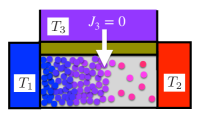
Figure 7: Operational interpretation of the global temperature $\tilde{T}$. A heat bath of $T_{3}$ contacts to the movable top plate. When $T_{3}=\tilde{T}$, the heat current $J_{3}$ from this heat bath may vanish. Then, the system behavior may be equivalent to the behavior of the original system in Fig. 2.

Moreover, we interpret ${\tilde{T}}$ from an operational viewpoint. We virtually attach another heat bath of the temperature $T_{3}$ to the rigid top plate as shown in Fig. 7. Using the idealized assumption that the motion of the top plate is sufficiently slower than the other dynamical degrees of freedom, we control $T_{1}$ and $T_{2}$ with $\Xi=T_{2}-T_{1}$ fixed such that the heat flux $J_{3}$ to the heat bath of $T_{3}$ is zero. Here, noting that the total kinetic energy in the bulk is given by $N_{\mathrm{deg}}k_{\mathrm{B}}{\tilde{T}}/2$ with the total degrees $N_{\mathrm{deg}}$ of freedom in the system, $J_{3}$ is proportional to ${\tilde{T}}-T_{3}$ in the linear response regime. That is, $J_{3}=0$ is equivalent to ${\tilde{T}}=T_{3}$. When we focus on the position of the top plate, the motion would be described as if it were in the equilibrium state at the temperature $T_{3}$. From this picture for the specific setting, it is expected that (5.12) is equivalent to the equilibrium variational principle with ${\tilde{T}}$.

As the last remark, we comment on the condition that $\Xi$ is fixed. Since there are two temperatures $T_{1}$ and $T_{2}$, two variables associated with $(T_{1},T_{2})$ should be fixed in the variation of $\cal X$. Although we adopt $\Xi$ as a fixed variable in addition to the global temperature $\tilde{T}$, one may conjecture that $J$ would be a more plausible fixed-variable than $\Xi$. As is formulated in (4.22), $J$ is proportional to $\Xi$ but the proportional constant depends on the interface position. Thus, the variational principle with $J$ fixed results in a different steady state from the solution of (5.10) with (5.11). There are two reasons for our choice. The first is that the final result becomes simplest among our trials. Second, when $J$ is fixed in the variation, the enthalpy is conserved in the variation. In this case, the corresponding variational principle may be an extension of the equilibrium variational principle for adiabatic (thermally isolated) systems. From these two aspects, we assume that $\Xi$ is fixed in the variation.

5.2 Steady state determined from the variational principle

We solve the variational equation (5.13). Hereafter, we consider the variation of ${\cal N}^{\mathrm{L}}$ with $({\tilde{T}},p^{\mathrm{ex}},\Xi)$ fixed. We abbreviate $A({\cal N}^{\mathrm{L}};{\tilde{T}},p^{\mathrm{ex}},\Xi)$ as $A({\cal N}^{\mathrm{L}})$ or $A$ for the notational simplicity.

We express the variational function $\cal G$ as

$${\cal G}({\cal N}^{\mathrm{L}})\equiv{F}^{\mathrm{L}}({\cal N}^{\mathrm{L}})+{F}^{\mathrm{G}}({\cal N}^{\mathrm{L}})+p^{\mathrm{ex}}V({\cal N}^{\mathrm{L}}),$$ (5.14)

where the free energy of the liquid $F^{\mathrm{L}}({\cal N}^{\mathrm{L}})$, the free energy of the gas $F^{\mathrm{G}}({\cal N}^{\mathrm{L}})$, and the volume of the system $V({\cal N}^{\mathrm{L}})$ are given as functions of ${\cal N}^{\mathrm{L}}$ with $({\tilde{T}},p^{\mathrm{ex}},\Xi)$ fixed. Here, for any global quantity $A$ in each region, such as ${\tilde{T}}^{\mathrm{L/G}}$ and $V^{\mathrm{L/G}}$, we define

$$\delta{A}\equiv{A}({\cal N}^{\mathrm{L}}+\delta{\cal N}^{\mathrm{L}})-{A}({\cal N}^{\mathrm{L}}).$$ (5.15)

We then have

$$\delta{\cal G}=\delta F^{\mathrm{L}}+\delta F^{\mathrm{G}}+p^{\mathrm{ex}}\delta V.$$ (5.16)

From the argument in §3, we obtain

$${F}^{\mathrm{L/G}}=F({\tilde{T}}^{\mathrm{L/G}},V^{\mathrm{L/G}},N^{\mathrm{L/G}}).$$ (5.17)

Since every global thermodynamic relation obtained in §3 holds in each region, we have

$${F}^{\mathrm{L/G}}=\tilde{\mu}^{\mathrm{L/G}}N^{\mathrm{L/G}}-p^{\mathrm{ex}}V^{\mathrm{L/G}}$$ (5.18)

with

$$\tilde{\mu}^{\mathrm{L/G}}=\mu^{\mathrm{L/G}}({\tilde{T}}^{\mathrm{L/G}},p^{\mathrm{ex}})+O(\varepsilon^{2}).$$ (5.19)

Since the variation of the free energy in each region obeys the fundamental relation of thermodynamics for $F$, we have

$$\delta F^{\mathrm{L/G}}=-S^{\mathrm{L/G}}\delta{\tilde{T}}^{\mathrm{L/G}}-p^{\mathrm{ex}}\delta V^{\mathrm{L/G}}+\tilde{\mu}^{\mathrm{L/G}}\delta{\cal N}^{\mathrm{L/G}},$$ (5.20)

where

$$S^{\mathrm{L/G}}={\cal N}^{\mathrm{L/G}}\hat{s}^{\mathrm{L/G}}({\tilde{T}}^{\mathrm{L/G}},p^{\mathrm{ex}})+O(\varepsilon^{2}).$$ (5.21)

By using (5.20), we rewrite the variation of ${\cal G}$ in (5.14) as

$$\delta{\cal G}=-S^{\mathrm{L}}\delta{\tilde{T}}^{\mathrm{L}}-S^{\mathrm{G}}\delta{\tilde{T}}^{\mathrm{G}}+(\tilde{\mu}^{\mathrm{L}}-\tilde{\mu}^{\mathrm{G}})\delta{\cal N}^{\mathrm{L}},$$ (5.22)

where we used ${\cal N}^{\mathrm{L}}+{\cal N}^{\mathrm{G}}=N$ and $V^{\mathrm{L}}+V^{\mathrm{G}}=V$.

The global temperature $\tilde{T}^{\mathrm{L}}$ in the liquid region and $\tilde{T}^{\mathrm{G}}$ in the gas region satisfy the relation

$$\tilde{T}^{\mathrm{L}}={\tilde{T}}-\frac{\Xi}{2}\frac{{\cal N}^{\mathrm{G}}}{N}+O(\varepsilon^{2}),\qquad\tilde{T}^{\mathrm{G}}={\tilde{T}}+\frac{\Xi}{2}\frac{{\cal N}^{\mathrm{L}}}{N}+O(\varepsilon^{2}),$$ (5.23)

which are derived from the relations

$${\tilde{T}}=\frac{{\cal N}^{\mathrm{L}}}{N}{\tilde{T}}^{\mathrm{L}}+\frac{{\cal N}^{\mathrm{G}}}{N}{\tilde{T}}^{\mathrm{G}},$$ (5.24)

and

$${\tilde{T}}^{\mathrm{G}}-{\tilde{T}}^{\mathrm{L}}=\frac{\Xi}{2}+O(\varepsilon^{2}).$$ (5.25)

Furthermore, (5.23) leads to

$$\delta{\tilde{T}}^{\mathrm{L}}=\delta{\tilde{T}}+\frac{\Xi}{2}\delta\left(\frac{{\cal N}^{\mathrm{L}}}{N}\right)-\frac{{\cal N}^{\mathrm{G}}}{2N}\delta\Xi,$$ (5.26)

$$\delta{\tilde{T}}^{\mathrm{G}}=\delta{\tilde{T}}+\frac{\Xi}{2}\delta\left(\frac{{\cal N}^{\mathrm{L}}}{N}\right)+\frac{{\cal N}^{\mathrm{L}}}{2N}\delta\Xi.$$ (5.27)

We have used ${\cal N}^{\mathrm{L}}+{\cal N}^{\mathrm{R}}=N$ in the first line. Especially, the formulas (5.26) and (5.27), with ${\tilde{T}}$, $\Xi$, and $N$ fixed, bring

$$\delta\tilde{T}^{\mathrm{L}}=\delta\tilde{T}^{\mathrm{G}}=\frac{\Xi}{2}\frac{\delta{\cal N}^{\mathrm{L}}}{N},$$ (5.28)

which simplifies (5.22) as

$$\delta{\cal G}=\left(\tilde{\mu}^{\mathrm{L}}-\frac{\Xi}{2N}S^{\mathrm{L}}-\tilde{\mu}^{\mathrm{G}}-\frac{\Xi}{2N}S^{\mathrm{G}}\right)\delta{\cal N}^{\mathrm{L}}.$$ (5.29)

Here, we confirm

$$\tilde{\mu}^{\mathrm{L}}-\frac{\Xi}{2N}S^{\mathrm{L}} =\mu^{\mathrm{L}}({\tilde{T}}^{\mathrm{L}},p^{\mathrm{ex}})+\frac{\Xi}{2}\frac{{\cal N}^{\mathrm{L}}}{N}\left(\frac{\partial\mu^{\mathrm{L}}}{\partial T}\right)_{p^{\mathrm{ex}}}+O(\varepsilon^{2})$$

$$=\mu^{\mathrm{L}}\left({\tilde{T}}^{\mathrm{L}}+\frac{\Xi}{2}\frac{{\cal N}^{\mathrm{L}}}{N},p^{\mathrm{ex}}\right)+O(\varepsilon^{2}),$$ (5.30)

and

$$\tilde{\mu}^{\mathrm{G}}+\frac{\Xi}{2N}S^{\mathrm{G}} =\mu^{\mathrm{G}}\left({\tilde{T}}^{\mathrm{G}}-\frac{\Xi}{2}\frac{{\cal N}^{\mathrm{G}}}{N},p^{\mathrm{ex}}\right)+O(\varepsilon^{2}).$$ (5.31)

Let us define a specific temperature $T^{\mathrm{s}}$ as

$$T^{\mathrm{s}}({\cal N}^{\mathrm{L}}) \equiv{\tilde{T}}+\Xi\left(\frac{{\cal N}^{\mathrm{L}}}{N}-\frac{1}{2}\right).$$ (5.32)

By using (5.23), we rewrite (5.32) as

$$T^{\mathrm{s}}({\cal N}^{\mathrm{L}}) ={\tilde{T}}^{\mathrm{L}}({\cal N}^{\mathrm{L}})+\frac{\Xi}{2}\frac{{\cal N}^{\mathrm{L}}}{N}={\tilde{T}}^{\mathrm{G}}({\cal N}^{\mathrm{L}})-\frac{\Xi}{2}\frac{{\cal N}^{\mathrm{G}}}{N}.$$ (5.33)

Thus, the variation (5.29) is further simplified as

$$\delta{\cal G}=\left(\mu^{\mathrm{L}}(T^{\mathrm{s}},p^{\mathrm{ex}})-\mu^{\mathrm{G}}(T^{\mathrm{s}},p^{\mathrm{ex}})+O(\varepsilon^{2})\right)\delta{\cal N}^{\mathrm{L}}.$$ (5.34)

This is equivalent to

$$\frac{\partial{\cal G}({\cal N}^{\mathrm{L}};{\tilde{T}},p^{\mathrm{ex}},\Xi)}{\partial{\cal N}^{\mathrm{L}}}=\mu^{\mathrm{L}}\left(T^{\mathrm{s}},p^{\mathrm{ex}}\right)-\mu^{\mathrm{G}}\left(T^{\mathrm{s}},p^{\mathrm{ex}}\right)+O(\varepsilon^{2}).$$ (5.35)

Since the functional form of $\mu^{\mathrm{G}}$ is different from that of $\mu^{\mathrm{L}}$ due to the crucial difference between the liquid and the gas, $\mu^{\mathrm{L}}\left(T^{\mathrm{s}},p^{\mathrm{ex}}\right)$ is not identically equal to $\mu^{\mathrm{G}}\left(T^{\mathrm{s}},p^{\mathrm{ex}}\right)$. The equality

$$\left.\mu^{\mathrm{L}}(T^{\mathrm{s}},p^{\mathrm{ex}})\right|_{{\cal N}^{\mathrm{L}}=N^{\mathrm{L}}}=\left.\mu^{\mathrm{G}}(T^{\mathrm{s}},p^{\mathrm{ex}})\right|_{{\cal N}^{\mathrm{L}}=N^{\mathrm{L}}}+O(\varepsilon^{2})$$ (5.36)

holds only when

$$\left.T^{\mathrm{s}}\right|_{{\cal N}^{\mathrm{L}}=N^{\mathrm{L}}}=T_{\mathrm{c}}(p^{\mathrm{ex}})+O(\varepsilon^{2}).$$ (5.37)

Now, (5.32) and (5.37) yield the unique value $N^{\mathrm{L}}$ as

$$\frac{N^{\mathrm{L}}({\tilde{T}},p^{\mathrm{ex}},\Xi)}{N}=\frac{1}{2}+\frac{T_{\mathrm{c}}(p^{\mathrm{ex}})-{\tilde{T}}}{\Xi}+O(\varepsilon).$$ (5.38)

Thus we conclude that the variational principle (5.13) results in the unique steady value $N^{\mathrm{L}}$ formulated by (5.38).

Next, we consider the second derivative of $\cal G$. By using (5.35) with (5.32), the second derivative of $\cal G$ is obtained as

$$\frac{\partial^{2}{\cal G}({\cal N}^{\mathrm{L}};{\tilde{T}},p^{\mathrm{ex}},\Xi)}{\partial({\cal N}^{\mathrm{L}})^{2}} =\left[\left(\frac{\partial\mu^{\mathrm{L}}}{\partial T^{\rm s}}\right)_{p^{\mathrm{ex}}}-\left(\frac{\partial\mu^{\mathrm{G}}}{\partial T^{\rm s}}\right)_{p^{\mathrm{ex}}}\right]\frac{dT^{\mathrm{s}}}{dN^{\mathrm{L}}}+O(\varepsilon^{2})$$

$$=(\hat{s}^{\mathrm{G}}(T^{\mathrm{s}},p^{\mathrm{ex}})-\hat{s}^{\mathrm{L}}(T^{\mathrm{s}},p^{\mathrm{ex}}))\frac{\Xi}{N}+O(\varepsilon^{2}).$$ (5.39)

At the steady state satisfying (5.37), the above entropy difference is connected to the latent heat $\hat{q}$ per one particle

$$\hat{q}(p^{\mathrm{ex}})=T_{\mathrm{c}}(p^{\mathrm{ex}})\left[\hat{s}^{\mathrm{G}}(T_{\mathrm{c}}(p^{\mathrm{ex}}),p^{\mathrm{ex}})-\hat{s}^{\mathrm{L}}(T_{\mathrm{c}}(p^{\mathrm{ex}}),p^{\mathrm{ex}})\right].$$ (5.40)

Therefore, we estimate the second derivative as

$$\left.\frac{\partial^{2}{\cal G}({\cal N}^{\mathrm{L}};{\tilde{T}},p^{\mathrm{ex}},\Xi)}{\partial({\cal N}^{\mathrm{L}})^{2}}\right|_{{\cal N}^{\mathrm{L}}=N^{\mathrm{L}}} =\frac{\hat{q}(p^{\mathrm{ex}})}{N}\frac{\Xi}{T_{\mathrm{c}}(p^{\mathrm{ex}})}+O(\varepsilon^{2}),$$ (5.41)

Since $\Xi>0$ and $\hat{q}(p^{\mathrm{ex}})>0$, we conclude that

$$\left.\frac{\partial^{2}{\cal G}({\cal N}^{\mathrm{L}};{\tilde{T}},p^{\mathrm{ex}},\Xi)}{\partial({\cal N}^{\mathrm{L}})^{2}}\right|_{{\cal N}^{\mathrm{L}}=N^{\mathrm{L}}}>0$$ (5.42)

in the linear response regime.

5.2.1 Careful analysis of $\varepsilon\to 0$

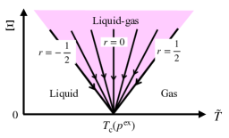
Figure 8: Phase diagram for a given $p^{\mathrm{ex}}$. For equilibrium cases ($\Xi=0$), the system shows the first-order transition at ${\tilde{T}}=T_{\mathrm{c}}(p^{\mathrm{ex}})$. The system is occupied by the liquid when ${\tilde{T}}>T_{\mathrm{c}}(p^{\mathrm{ex}})-{\Xi}/{2}$ and by the gas when ${\tilde{T}}<T_{\mathrm{c}}(p^{\mathrm{ex}})+{\Xi}/{2}$. The liquid and the gas coexist when $\Xi>0$ and $T_{\mathrm{c}}(p^{\mathrm{ex}})-{\Xi}/{2}<{\tilde{T}}<T_{\mathrm{c}}(p^{\mathrm{ex}})+{\Xi}/{2}$ painted by pink. The ratio of the liquid and the gas is kept along the line corresponding to each value of $r$, which goes to $T=T_{\mathrm{c}}(p^{\mathrm{ex}})$ at $\Xi=0$.

The solution (5.38) of the variational principle includes an undetermined term of $O(\varepsilon)$. Nevertheless, (5.38) provides additional information to equilibrium behavior. To clarify the situation, we consider the limit $\varepsilon\to 0$ with keeping the phase coexistence. This may be formalized by fixing a parameter $r$ defined as

$$r\equiv\frac{{\tilde{T}}-T_{\mathrm{c}}(p^{\mathrm{ex}})}{\Xi},$$ (5.43)

whereas (5.38) indicates

$$\frac{N^{\mathrm{L}}}{N}=\frac{1}{2}-r.$$ (5.44)

As $0<N^{\mathrm{L}}<N$, $r$ satisfies

$$-\frac{1}{2}<r<\frac{1}{2}.$$ (5.45)

In Fig. 8, we draw straight lines connecting from $({\tilde{T}},\Xi)=(T_{\mathrm{c}}+r\Xi,\Xi)$ to $(T_{\mathrm{c}},0)$ for several values of $r$ in the parameter region where the liquid-gas coexistence is observed. The convergence of these lines at $(T_{\mathrm{c}},0)$ indicates that the equilibrium state $(T_{\mathrm{c}},0)$ behaves as a singular point. By specifying the value of $r$, we identify the corresponding line which undoes the degeneration at equilibrium. $N^{\mathrm{L}}$ is determined by considering the equilibrium limit $\varepsilon\rightarrow 0$, while it is not uniquely determined at equilibrium.

5.3 Temperature relation

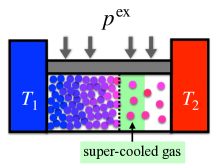
Figure 9: Super-cooled gas stabilized by the steady heat current.

We obtained the steady state value of $N^{\mathrm{L}}$ as (5.38) by solving the variational principle (5.13). Substituting this solution into (5.33) with (5.37), we have the global temperature for each region as

$${\tilde{T}}^{\mathrm{L/G}}({\tilde{T}},p^{\mathrm{ex}},\Xi)=\frac{T_{\mathrm{c}}(p^{\mathrm{ex}})+{\tilde{T}}}{2}\mp\frac{\Xi}{4}+O(\varepsilon^{2}).$$ (5.46)

We sum up the two relations in (5.46) and substitute (4.27) into ${\tilde{T}}^{\mathrm{L/G}}$. We then obtain

$${\tilde{T}}-{T_{\mathrm{m}}}=\theta-T_{\mathrm{c}}(p^{\mathrm{ex}})+O(\varepsilon^{2}),$$ (5.47)

which we call the temperature relation. This non-trivial relation, which results from the variational principle, is a simple condition that the steady states satisfy. Generally, ${\tilde{T}}$ is not equal to ${T_{\mathrm{m}}}$, because the particle density of liquid is larger than that of gas, $\rho^{\mathrm{L}}>\rho^{\mathrm{G}}$. Therefore, the relation (5.47) implies that the liquid-gas coexistence temperature $\theta$ in a heat conduction system must be strictly lower than the equilibrium coexistence temperature $T_{\mathrm{c}}(p^{\mathrm{ex}})$. This means that metastable states stably appear near the liquid-gas interface as schematically shown in Fig. 9.

Now, suppose that (5.47) holds. Summing up the two equalities in (5.23), we obtain

$$T_{\mathrm{m}}+\theta=2{\tilde{T}}+\frac{\Xi}{2}\left(\frac{2N^{\mathrm{L}}}{N}-1\right).$$ (5.48)

Here, it should be noted that we do not use the variational principle for the derivation of (5.23). By substituting the temperature relation (5.47) into this result, we derive (5.38) without the variational principle. In this sense, we may say that the temperature relation (5.47) is equivalent to the variational principle.

5.4 Global quantities as functions of $({\tilde{T}},p^{\mathrm{ex}},\Xi)$

We determine the steady state values of several quantities. Let $V_{\mathrm{s}}^{\mathrm{L/G}}(p^{\mathrm{ex}})$ denote the equilibrium saturated volume defined as

$$V_{\mathrm{s}}^{\mathrm{L/G}}(p^{\mathrm{ex}})=\frac{N}{\rho^{\mathrm{L/G}}_{\mathrm{c}}(p^{\mathrm{ex}})}$$ (5.49)

with

$$\rho^{\mathrm{L/G}}_{\mathrm{c}}(p^{\mathrm{ex}})=\rho^{\mathrm{L/G}}(T_{\mathrm{c}}(p^{\mathrm{ex}}),p^{\mathrm{ex}}).$$ (5.50)

The volume of the liquid (gas) region is given by

$$V^{\mathrm{L/G}}({\tilde{T}},p^{\mathrm{ex}},\Xi) =\frac{N^{\mathrm{L/G}}}{N}V_{\mathrm{s}}^{\mathrm{L/G}}(p^{\mathrm{ex}})+O(\varepsilon).$$ (5.51)

Since $N^{\mathrm{L}}$ is determined with an error of $O(\varepsilon)$ in (5.38), (5.51) is the best estimate of $V^{\mathrm{L/G}}$ in $\varepsilon\rightarrow 0$. Substituting (5.38) into (5.51), we obtain

$$V({\tilde{T}},p^{\mathrm{ex}},\Xi)$$

$$=\left(\frac{1}{2}-\frac{{\tilde{T}}-T_{\mathrm{c}}(p^{\mathrm{ex}})}{\Xi}\right)V_{\mathrm{s}}^{\mathrm{L}}(p^{\mathrm{ex}})+\left(\frac{1}{2}+\frac{{\tilde{T}}-T_{\mathrm{c}}(p^{\mathrm{ex}})}{\Xi}\right)V_{\mathrm{s}}^{\mathrm{G}}(p^{\mathrm{ex}})+O(\varepsilon).$$ (5.52)

which corresponds to the solution of the variational principle (5.10). Then, the steady position $X$ of the liquid-gas interface,

$$\frac{X}{L_{x}}=\frac{V^{\mathrm{L}}}{V},$$ (5.53)

is determined as

$$\frac{X({\tilde{T}},p^{\mathrm{ex}},\Xi)}{L_{x}}=\frac{\displaystyle\frac{1}{2}-\frac{{\tilde{T}}-T_{\mathrm{c}}(p^{\mathrm{ex}})}{\Xi}}{\displaystyle\frac{1}{2}\left(\frac{\rho^{\mathrm{L}}_{\mathrm{c}}}{\rho^{\mathrm{G}}_{\mathrm{c}}}+1\right)+\frac{{\tilde{T}}-T_{\mathrm{c}}(p^{\mathrm{ex}})}{\Xi}\left(\frac{\rho^{\mathrm{L}}_{\mathrm{c}}}{\rho^{\mathrm{G}}_{\mathrm{c}}}-1\right)}+O(\varepsilon),$$ (5.54)

which is the solution of the variational principle (5.12).

Then, the interface temperature is obtained from the elimination of $T_{\mathrm{m}}$ from (5.47) and (4.20) as

$$\theta({\tilde{T}},p^{\mathrm{ex}},\Xi)=\frac{T_{\mathrm{c}}(p^{\mathrm{ex}})+{\tilde{T}}}{2}+\frac{\Xi}{4}\left(\frac{X}{\kappa^{\mathrm{L}}_{\mathrm{c}}}-\frac{L_{x}-X}{\kappa^{\mathrm{G}}_{\mathrm{c}}}\right)\left(\frac{X}{\kappa^{\mathrm{L}}_{\mathrm{c}}}+\frac{L_{x}-X}{\kappa^{\mathrm{G}}_{\mathrm{c}}}\right)^{-1}+O(\varepsilon^{2}).$$ (5.55)

The deviation of $\theta$ from $T_{\mathrm{c}}$ and the relation between $X$ and $\theta$ will be demonstrated in §6 for explicit examples.

6 Properties of the steady states with a liquid-gas interface

In §5.4, we derived the steady state values for given $({\tilde{T}},\Xi)$ such as $N^{\mathrm{L}}=N^{\mathrm{L}}({\tilde{T}},p^{\mathrm{ex}},\Xi)$ in (5.38), $V=V({\tilde{T}},p^{\mathrm{ex}},\Xi)$ in (5.52) and $X=X({\tilde{T}},p^{\mathrm{ex}},\Xi)$ in (5.54). However, the global temperature ${\tilde{T}}$ is not easily controlled in experiments, differently from the heat bath temperatures $T_{1}$ and $T_{2}$. In this section, we express any quantity in the steady state as a function of $(T_{1},T_{2},p^{\mathrm{ex}})$. In §6.1, we derive $(\tilde{T},X)$ as a function of $(T_{1},T_{2},p^{\mathrm{ex}})$. Since we already have

$$A=A(X;{\tilde{T}},p^{\mathrm{ex}},\Xi),$$ (6.1)

the relations

$${\tilde{T}} ={\tilde{T}}(T_{1},T_{2},p^{\mathrm{ex}}),$$ (6.2)

$$X =X(T_{1},T_{2},p^{\mathrm{ex}}),$$ (6.3)

lead to the expression

$$A=A(T_{1},T_{2},p^{\mathrm{ex}},\Xi).$$ (6.4)

Particularly, we consider the interface temperature $\theta$ and the jump of the chemical potential $\Delta\mu$ at the interface as a function of $(T_{1},T_{2},p^{\mathrm{ex}})$ in §6.2 as (6.12) and §6.3 as (6.27), respectively. In §6.4, we discuss how the super-cooled gas appears near the interface quantitatively. The last subsection §6.5 is devoted to the demonstration of examples. In what follows, we use the notations

$$u\equiv\frac{\rho^{\mathrm{L}}_{\mathrm{c}}(p^{\mathrm{ex}})}{\rho^{\mathrm{G}}_{\mathrm{c}}(p^{\mathrm{ex}})},\qquad v\equiv\frac{\kappa^{\mathrm{L}}_{\mathrm{c}}(p^{\mathrm{ex}})}{\kappa^{\mathrm{G}}_{\mathrm{c}}(p^{\mathrm{ex}})},\qquad\zeta\equiv\frac{X}{L_{x}}$$ (6.5)

for simplicity.

6.1 $\tilde{T}$ and $\zeta$ as functions of $(T_{1},T_{2},p^{\mathrm{ex}})$

Substituting (5.55) into (5.47), we obtain

$${\tilde{T}}=2T_{\mathrm{m}}-T_{\mathrm{c}}(p^{\mathrm{ex}})+\frac{\Xi}{2}\frac{\zeta-v(1-\zeta)}{\zeta+v(1-\zeta)}+O(\varepsilon^{2}),$$ (6.6)

where the dimensionless position $\zeta$ of the steady interface is

$$\zeta=\frac{\displaystyle\frac{1}{2}-\frac{{\tilde{T}}-T_{\mathrm{c}}(p^{\mathrm{ex}})}{\Xi}}{\displaystyle\frac{1}{2}\left(1+u\right)-\frac{{\tilde{T}}-T_{\mathrm{c}}(p^{\mathrm{ex}})}{\Xi}\left(1-u\right)}+O(\varepsilon),$$ (6.7)

as is derived in (5.54). Eliminating ${\tilde{T}}$ from (6.6) and (6.7), we have

$$T_{\mathrm{m}}-T_{\mathrm{c}}(p^{\mathrm{ex}})=-\frac{\Xi}{2}\frac{u\zeta^{2}-v(1-\zeta)^{2}}{[u\zeta+(1-\zeta)][\zeta+v(1-\zeta)]}+O(\varepsilon^{2}).$$ (6.8)

Solving this equation in $\zeta$, we derive

$$\zeta(T_{1},T_{2},p^{\mathrm{ex}})=\frac{tu+(1-t)v+t(u-1)(v-1)-\sqrt{(uv-1)^{2}t^{2}+uv}}{v-u+2t(u-1)(v-1)}+O(\varepsilon),$$ (6.9)

with

$$t\equiv\frac{T_{\mathrm{m}}-T_{\mathrm{c}}(p^{\mathrm{ex}})}{\Xi}.$$ (6.10)

(6.9) provides a concrete functional form of (6.3).

Substituting (6.8) into (6.6), we obtain a concrete form of (6.2),

$${\tilde{T}}(T_{1},T_{2},p^{\mathrm{ex}})=T_{\mathrm{m}}-\frac{\Xi}{2}\frac{(uv-1)\zeta(1-\zeta)}{[u\zeta+(1-\zeta)][\zeta+v(1-\zeta)]}+O(\varepsilon^{2}),$$ (6.11)

with the form of $\zeta$ in (6.9).

6.2 Interface temperature as a function of $(T_{1},T_{2},p^{\mathrm{ex}})$

Applying the temperature relation (5.47) to (6.11), we find that the interface temperature is written as

$$\theta(T_{1},T_{2},p^{\mathrm{ex}})=T_{\mathrm{c}}(p^{\mathrm{ex}})-\frac{\Xi}{2}\frac{(uv-1)\zeta(1-\zeta)}{[u\zeta+(1-\zeta)][\zeta+v(1-\zeta)]}+O(\varepsilon^{2}),$$ (6.12)

where $\zeta$ is given by (6.9). This formula clarifies that the interface temperature $\theta(T_{1},T_{2},p^{\mathrm{ex}})$ generally deviates from $T_{\mathrm{c}}(p^{\mathrm{ex}})$ when the temperature gradient is imposed. Since the particle density satisfies $\rho^{\mathrm{L}}>\rho^{\mathrm{G}}$, i.e., $u>1$, and the heat conductivity is expected to be $\kappa^{\mathrm{L}}\neq\kappa^{\mathrm{G}}$, the interface temperature $\theta$ is deviated from the equilibrium transition temperature $T_{\mathrm{c}}(p^{\mathrm{ex}})$ in the order of $\varepsilon$, which is not negligible.

We have another formula for the interface temperature $\theta$, which is expressed solely by experimentally accessible quantities:

$$\theta=T_{\mathrm{c}}(p^{\mathrm{ex}})-\frac{\zeta(1-\zeta)}{2}\left[-JL_{x}\left(\frac{1}{\kappa^{\mathrm{G}}_{\mathrm{c}}}-\frac{1}{\kappa^{\mathrm{L}}_{\mathrm{c}}}\right)+\Xi\bar{\phi}\left(\rho^{\mathrm{L}}_{\mathrm{c}}-{\rho^{\mathrm{G}}_{\mathrm{c}}}\right)\right]+O(\varepsilon^{2}),$$ (6.13)

where $\bar{\phi}=V/N$. The derivation of this formula is shown in §6.2.1.

Up to here, we have studied the systems with $T_{1}<T_{2}$, where $\Xi>0$ and $J<0$. More generally, from the left-right symmetry of the system in Fig. 2, we notice that the interface temperature is invariant for the transformation $(\Xi,\zeta)$ to $(-\Xi,1-\zeta)$. That is, (6.13) is expressed as

$$\theta=T_{\mathrm{c}}(p^{\mathrm{ex}})-\frac{\zeta(1-\zeta)}{2}\left[|J|L_{x}\left(\frac{1}{\kappa^{\mathrm{G}}_{\mathrm{c}}}-\frac{1}{\kappa^{\mathrm{L}}_{\mathrm{c}}}\right)+|\Xi|\bar{\phi}\left(\rho^{\mathrm{L}}_{\mathrm{c}}-{\rho^{\mathrm{G}}_{\mathrm{c}}}\right)\right]+O(\varepsilon^{2})$$ (6.14)

for any $\Xi$.

One might guess that the coexistence temperature $\theta$ is uniquely determined by local quantities that characterize the phase boundary, namely, the pressure $p^{\mathrm{ex}}$ and the heat current per unit area. Rather interestingly, this is not the case. Reflecting the global nature of our variational principle, the coexistence temperature $\theta$ explicitly depends on global conditions of the system, namely, the temperatures of the two heat baths.

6.2.1 Derivetion of (6.13)

We first recall (4.19) and (4.20). From these,

$$\Xi=-JL_{x}\left(\frac{\zeta}{\kappa^{\mathrm{L}}_{\mathrm{c}}}+\frac{1-\zeta}{\kappa^{\mathrm{G}}_{\mathrm{c}}}\right)+O(\varepsilon^{2}),$$ (6.15)

$$T_{\mathrm{m}}-\theta=\frac{JL_{x}}{2}\left(\frac{\zeta}{\kappa^{\mathrm{L}}_{\mathrm{c}}}-\frac{1-\zeta}{\kappa^{\mathrm{G}}_{\mathrm{c}}}\right)+O(\varepsilon^{2}).$$ (6.16)

Combining these two relations, we have another form of $T_{\mathrm{m}}$ as

$$T_{\mathrm{m}}-\theta=\frac{\Xi}{2}+\zeta\frac{JL_{x}}{\kappa^{\mathrm{L}}_{\mathrm{c}}}=-\frac{\Xi}{2}-(1-\zeta)\frac{JL_{x}}{\kappa^{\mathrm{G}}_{\mathrm{c}}}$$ (6.17)

with an error of $O(\varepsilon^{2})$.

Second, the result of the variational principle (5.38) is written as

$${\tilde{T}}-T_{\mathrm{c}}(p^{\mathrm{ex}})=\frac{\Xi}{2}-\Xi\frac{N^{\mathrm{L}}}{N}+O(\varepsilon^{2})=-\frac{\Xi}{2}+\Xi\frac{N^{\mathrm{G}}}{N}+O(\varepsilon^{2}).$$ (6.18)

As $N^{\mathrm{L}}=\zeta V\rho^{\mathrm{L}}(\tilde{T}^{\mathrm{L}},p^{\mathrm{ex}})$ and $N^{\mathrm{G}}=(1-\zeta)V\rho^{\mathrm{G}}(\tilde{T}^{\mathrm{G}},p^{\mathrm{ex}})$ with $\rho^{\mathrm{L}}(\tilde{T}^{\mathrm{L}},p^{\mathrm{ex}})=\rho^{\mathrm{L}}_{\mathrm{c}}+O(\varepsilon)$ and $\rho^{\mathrm{G}}(\tilde{T}^{\mathrm{G}},P)=\rho^{\mathrm{G}}_{\mathrm{c}}+O(\varepsilon)$, the relation (6.18) is further expressed as

$${\tilde{T}}-T_{\mathrm{c}}(p^{\mathrm{ex}})=\frac{\Xi}{2}-\zeta\Xi\bar{\phi}\rho^{\mathrm{L}}_{\mathrm{c}}=-\frac{\Xi}{2}+(1-\zeta)\Xi\bar{\phi}\rho^{\mathrm{G}}_{\mathrm{c}}$$ (6.19)

with an error of $O(\varepsilon^{2})$. By subtracting (6.17) from (6.19) and using the temperature relation (5.47), we have two forms of the interface temperature:

$$\theta-T_{\mathrm{c}}(p^{\mathrm{ex}}) =-\frac{\zeta}{2}\left(\frac{JL_{x}}{\kappa^{\mathrm{L}}_{\mathrm{c}}}+\Xi\bar{\phi}\rho^{\mathrm{L}}_{\mathrm{c}}\right),$$ (6.20)

$$\theta-T_{\mathrm{c}}(p^{\mathrm{ex}}) =\frac{1-\zeta}{2}\left(\frac{JL_{x}}{\kappa^{\mathrm{G}}_{\mathrm{c}}}+\Xi\bar{\phi}\rho^{\mathrm{G}}_{\mathrm{c}}\right).$$ (6.21)

By substituting (6.20) and (6.21) into the first term and the second term of the right-hand side of the trivial identity

$$\theta-T_{\mathrm{c}}(p^{\mathrm{ex}})=(1-\zeta)(\theta-T_{\mathrm{c}}(p^{\mathrm{ex}}))+\zeta(\theta-T_{\mathrm{c}}(p^{\mathrm{ex}})),$$ (6.22)

we obtain (6.13).

6.3 $\Delta\mu$ as a function of $(T_{1},T_{2},p^{\mathrm{ex}})$

Next, we discuss the chemical potential jump

$$\Delta\mu\equiv\mu^{\mathrm{G}}(\theta,p^{\mathrm{ex}})-\mu^{\mathrm{L}}(\theta,p^{\mathrm{ex}})$$ (6.23)

at the interface. Note that

$$\mu^{\mathrm{G}}(T_{\mathrm{c}}(p^{\mathrm{ex}}),p^{\mathrm{ex}})=\mu^{\mathrm{L}}(T_{\mathrm{c}}(p^{\mathrm{ex}}),p^{\mathrm{ex}}),$$ (6.24)

which gives the definition of the transition temperature $T_{\mathrm{c}}$. Thus, $\theta\not=T_{\mathrm{c}}$ means the imbalance of the chemical potential at the interface, which is quantitatively expressed as

$$\Delta\mu=-[\hat{s}^{\mathrm{G}}(T_{\mathrm{c}}(p^{\mathrm{ex}}),p^{\mathrm{ex}})-\hat{s}^{\mathrm{L}}(T_{\mathrm{c}}(p^{\mathrm{ex}}),p^{\mathrm{ex}})](\theta-T_{\mathrm{c}}(p^{\mathrm{ex}}))+O(\varepsilon^{2}).$$ (6.25)

Since the entropy difference is connected to the latent heat $\hat{q}$ per one particle as

$$\hat{s}^{\mathrm{G}}(T_{\mathrm{c}}(p^{\mathrm{ex}}),p^{\mathrm{ex}})-\hat{s}^{\mathrm{L}}(T_{\mathrm{c}}(p^{\mathrm{ex}}),p^{\mathrm{ex}})=\frac{\hat{q}}{T_{\mathrm{c}}(p^{\mathrm{ex}})},$$ (6.26)

the jump of the chemical potential is proportional to $\hat{q}$. Now, substituting (6.12) into (6.25), the amount of the jump is estimated as

$$\Delta\mu =\frac{\hat{q}}{2}\frac{\Xi}{T_{\mathrm{c}}(p^{\mathrm{ex}})}\frac{(uv-1)\zeta(1-\zeta)}{[u\zeta+(1-\zeta)][\zeta+v(1-\zeta)]}+O(\varepsilon^{2}),$$ (6.27)

Another expression of $\Delta\mu$ is also obtained by substituting (6.13) into (6.25). The result is

$$\Delta\mu =\frac{\zeta(1-\zeta)}{2}\frac{\hat{q}}{T_{\mathrm{c}}(p^{\mathrm{ex}})}\left[-JL_{x}\left(\frac{1}{\kappa^{\mathrm{G}}_{\mathrm{c}}}-\frac{1}{\kappa^{\mathrm{L}}_{\mathrm{c}}}\right)+\Xi\bar{\phi}\left(\rho^{\mathrm{L}}_{\mathrm{c}}-{\rho^{\mathrm{G}}_{\mathrm{c}}}\right)\right]+O(\varepsilon^{2}).$$ (6.28)

6.4 Super-cooled gas in the liquid-gas coexistence

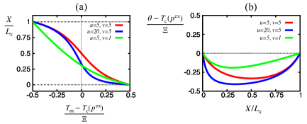
Figure 10: Theoretical results for the parameter values $(u,v)=(5,5)$, $(20,5)$ and $(5,1)$. (a) The position of the liquid-gas interface in (6.9) when $T_{\mathrm{m}}$ deviates from $T_{\mathrm{c}}(p^{\mathrm{ex}})$. (b) The deviation of the interface temperature $\theta$ in (6.12). All the three cases show $\theta<T_{\mathrm{c}}(p^{\mathrm{ex}})$, which indicates the stabilization of the super-cooled gas near the interface in the heat conduction.

When $T_{1}<T_{\mathrm{c}}(p^{\mathrm{ex}})<T_{2}$, we find the position $X_{\mathrm{c}}$ at which the local temperature satisfies $T(X_{\mathrm{c}};T_{1},T_{2},p^{\mathrm{ex}})=T_{\mathrm{c}}(p^{\mathrm{ex}})$. Suppose $\theta<T_{\mathrm{c}}(p^{\mathrm{ex}})$. Then, the position $X$ of the interface satisfies

$$0<X<X_{\mathrm{c}}<L_{x}.$$ (6.29)

We observe the liquid in the region $0<x<X$ and the gas in $X<x<L_{x}$. Then the local temperature of the gas in $X<x<X_{\mathrm{c}}$ is less than $T_{\mathrm{c}}(p^{\mathrm{ex}})$. This means that a super-cooled gas is observed in $X<x<X_{\mathrm{c}}$, which is not stable in equilibrium.

We plot (6.9) and (6.12) in Fig. 10 for three sets of $(u,v)$. It is clearly seen that the interface temperature $\theta$ deviates from the equilibrium transition temperature $T_{\mathrm{c}}(p^{\mathrm{ex}})$. The deviation of the global temperature ${\tilde{T}}$ from $T_{\mathrm{m}}$ shows the same figure with Fig. 10(b) due to the temperature relation (5.47). The jump of the chemical potential at the interface also exhibits the same dependence on $\zeta=X/L_{x}$ since it is proportional to $\theta-T_{\mathrm{c}}(p^{\mathrm{ex}})$ as shown in (6.27). In the presented three sets of $(u,v)$, a super-cooled gas region appears near the right side of the interface, as shown schematically in Fig. 9.

According to Fig.  10(a), the stable position of the interface is shifted continuously as we increase the temperature of both heat baths. This feature is different from the numerical solution of the variational equation reported in Ref. NS , where the interface discontinuously appears. A more accurate numerical calculation was necessary for the cases with high $\rho^{\mathrm{L}}_{\mathrm{c}}/\rho^{\mathrm{G}}_{\mathrm{c}}$.

6.5 Examples

In this subsection, we illustrate some examples of the liquid-gas coexistence in heat conduction quantitatively, where the particle density is measured in mol.

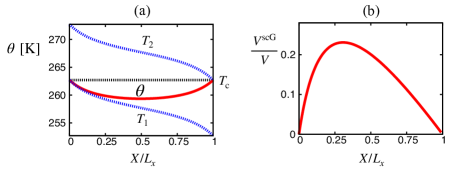
Figure 11: (a) The interface temperature $\theta$ and (b) volume fraction of the super-cooled gas for ${\rm CO}_{2}$ under $p^{\mathrm{ex}}=4\times 10^{6}$ Pa. $\Xi=10$ K. See the main text for parameter values. In (a), $\theta$ (red solid line), $T_{\mathrm{c}}$ (black dotted line), $T_{1}$ and $T_{2}$ (blue dotted lines) are depicted simultaneously as a function of the interface position.

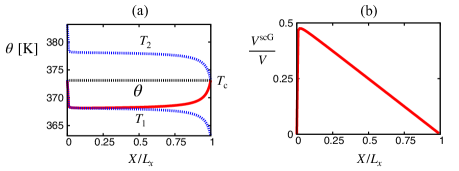
Figure 12: (a) The interface temperature $\theta$ and (b) volume fraction of the super-cooled gas for ${\rm H}_{2}{\rm O}$ under $p^{\mathrm{ex}}=1.013\times 10^{5}$ Pa. $\Xi=10$ K. See the main text for parameter values. In (a), $\theta$ (red solid line), $T_{\mathrm{c}}$ (black dotted line), $T_{1}$ and $T_{2}$ (blue dotted lines) are depicted simultaneously as a function of the interface position.

First, we consider the van der Waals equation of state

$$p=\frac{RT\rho}{1-b\rho}-a\rho^{2}$$ (6.30)

of $a=0.365$ Pa$\cdot$ m⁶/mol² and $b=4.28\times 10^{-5}$ m³/mol for ${\rm CO}_{2}$ at a high pressure $p^{\mathrm{ex}}=4\times 10^{6}$ Pa CO2 . The gas constant is $R=8.31$ J/K$\cdot$mol. Substituting these parameters into (6.30), we obtain the transition temperature as $T_{\mathrm{c}}=262.7$ K, and the mol density at $T_{\mathrm{c}}$ as $\rho^{\mathrm{L}}_{\mathrm{c}}=1.38\times 10^{4}$ mol/m³ and $\rho^{\mathrm{G}}_{\mathrm{c}}=2.70\times 10^{3}$ mol/m³, which results in $u=5.1$. From the database NIST , we set the heat conductivity of the liquid as $\kappa^{\mathrm{L}}=0.1$ W/m$\cdot$ K and that of the gas as $\kappa^{\mathrm{G}}=0.02$ W/m$\cdot$ K, which yields $v=5$. The result is close to the result $(u,v)=(5.5)$ which was already shown in Fig.  10. The temperature profile becomes linear both in the liquid and gas regions in this example due to the constant heat conductivity. Then the volume fraction of the super-cooled gas is simply obtained as

$$\frac{V^{\mathrm{scG}}}{V}=\frac{L_{x}-X}{L_{x}}\frac{T_{\mathrm{c}}-\theta(X)}{T_{2}(X)-\theta(X)},$$ (6.31)

where $V^{\mathrm{scG}}$ is the volume of the super-cooled gas, i.e., $V^{\rm scG}=(X-X_{\mathrm{c}})/L_{x}$. The interface temperature $\theta(X)$ is given by (6.12) and $T_{2}$ results from (6.8) as

$$T_{2}(X)=T_{\mathrm{c}}(p^{\mathrm{ex}})+\frac{\Xi}{2}-\frac{\Xi}{2}\frac{u\zeta^{2}-v(1-\zeta)^{2}}{[u\zeta+(1-\zeta)][\zeta+v(1-\zeta)]}+O(\varepsilon^{2}),$$ (6.32)

where $\zeta=X/L_{x}$. In Fig. 11, we show the interface temperature $\theta$ and the volume fraction $V^{\mathrm{scG}}/V$ as a function of the position of the interface when $\Xi=10$ K. We notice that the interface temperature $\theta$ may deviate about $3.3$ K from $T_{\mathrm{c}}$, and that the volume fraction of the super-cooled gas may exceed $1/3$.

Second, more importantly, we do not need the equation of state, but have only to know the value of $u$, $v$, $T_{\mathrm{c}}(p^{\mathrm{ex}})$, when we obtain the phase diagram for a given material. For example, consider pure water at $1.013\times 10^{5}$ Pa, where $T_{\mathrm{c}}(p^{\mathrm{ex}})=373.1$ K. From the database NIST , we have $u=1604$ and $v=27.06$. From these, we can predict the interface temperature $\theta$ and the volume fraction $V^{\mathrm{scG}}/V$ as a function of the position of the interface as shown in Fig. 12. As an example, when $T_{1}=368.0$ K and $T_{2}=378.0$ K, we obtain $\theta=368.3$ K and $X/L_{x}=0.4086$.

7 Global thermodynamics for systems with a liquid-gas interface

Hereafter, all the quantities are defined in the steady state. When a global quantity ${A}$ is determined for $({\tilde{T}},p,N,\Xi)$, we express this relation as

$${A}=A({\tilde{T}},p,N,\Xi).$$ (7.1)

Recall that $A({\tilde{T}},p,N,\Xi)=A({\tilde{T}},p,N)+O(\varepsilon^{2})$ for single-phase systems, where $A({\tilde{T}},P,N)$ is the equilibrium function, as discussed in §3. For the systems with a liquid-gas interface, $\Xi$ dependence appears even in the linear response regime. In this section, we extend the global thermodynamics introduced in §3 so as to describe the liquid-gas coexistence determined in the previous sections. In §7.1, we derive formulas as preliminaries for later sections. In §7.2, we formally derive a fundamental relation of thermodynamics for systems with a liquid-gas interface. However, since the derivative of $G$ is not defined at $(T_{\mathrm{c}}(p),p)$, the formal expression is not properly defined. Then, in §7.3, we perform a careful analysis of the limit $\varepsilon\to 0$. In §7.4, we show the form of the entropy and the volume in the appropriate limit. In §7.5, we present formulas for constant pressure heat capacity and compressibility.

7.1 Preliminaries

We first study global extensive quantities

$${A}=L_{y}L_{z}\int_{0}^{L_{x}}dx~{}a(T(x),p).$$ (7.2)

It is obvious that they possess the additivity

$${A}={A}^{\mathrm{L}}+{A}^{\mathrm{G}},$$ (7.3)

where ${A}^{\mathrm{L}}$ and ${A}^{\mathrm{G}}$ are defined as global thermodynamic quantities in the liquid region and the gas region, respectively. By using ${\tilde{T}}^{\mathrm{L}}$ and ${\tilde{T}}^{\mathrm{G}}$, we write

$${A}^{\mathrm{L}}=N^{\mathrm{L}}\hat{a}^{\mathrm{L}}({\tilde{T}}^{\mathrm{L}},p)+O(\varepsilon^{2}),$$ (7.4)

$${A}^{\mathrm{G}}=N^{\mathrm{G}}\hat{a}^{\mathrm{G}}({\tilde{T}}^{\mathrm{G}},p)+O(\varepsilon^{2}).$$ (7.5)

Now, we consider an infinitely small change $(T_{1},T_{2},p,N)\rightarrow(T_{1}+\delta T_{1},T_{2}+\delta T_{2},p+\delta p,N+\delta N)$, which results in

$$({\tilde{T}},p,N,\Xi)\to({\tilde{T}}+\delta{\tilde{T}},p+\delta p,N+\delta N,\Xi+\delta\Xi).$$ (7.6)

Accordingly, any quantity $\phi$ for the steady state $({\tilde{T}},p,N,\Xi)$ changes as

$$\delta\phi=\phi({\tilde{T}}+\delta{\tilde{T}},p+\delta p,N+\delta N,\Xi+\delta\Xi)-\phi({\tilde{T}},p,N,\Xi).$$ (7.7)

Then, (7.4) and (7.5) bring the following relations among the infinitely small changes:

$$\delta{A}^{\mathrm{L}} =N^{\mathrm{L}}\left(\frac{\partial\hat{a}^{\mathrm{L}}}{\partial{\tilde{T}}^{\mathrm{L}}}\right)_{p}\delta{\tilde{T}}^{\mathrm{L}}+N^{\mathrm{L}}\left(\frac{\partial\hat{a}^{\mathrm{L}}}{\partial p}\right)_{{\tilde{T}}^{\mathrm{L}}}\delta p+\hat{a}^{\mathrm{L}}\delta N^{\mathrm{L}}+O(\varepsilon^{2}),$$ (7.8)

$$\delta{A}^{\mathrm{G}} =N^{\mathrm{G}}\left(\frac{\partial\hat{a}^{\mathrm{G}}}{\partial{\tilde{T}}^{\mathrm{G}}}\right)_{p}\delta{\tilde{T}}^{\mathrm{G}}+N^{\mathrm{G}}\left(\frac{\partial\hat{a}^{\mathrm{G}}}{\partial P}\right)_{{\tilde{T}}^{\mathrm{G}}}\delta p+\hat{a}^{\mathrm{G}}\delta N^{\mathrm{G}}+O(\varepsilon^{2}).$$ (7.9)

We sum up the above two relations (7.8) and (7.9) and substitute (5.26) and (5.27) into them. Then, the sum becomes

$$\delta{A} =\left(N^{\mathrm{L}}\left(\frac{\partial\hat{a}^{\mathrm{L}}}{\partial{\tilde{T}}^{\mathrm{L}}}\right)_{p}+N^{\mathrm{G}}\left(\frac{\partial\hat{a}^{\mathrm{G}}}{\partial{\tilde{T}}^{\mathrm{G}}}\right)_{p}\right)\left(\delta{\tilde{T}}+\frac{\Xi}{2}\delta\left(\frac{N^{\mathrm{L}}}{N}\right)\right)$$

$$+\left(N^{\mathrm{L}}\left(\frac{\partial\hat{a}^{\mathrm{L}}}{\partial p}\right)_{{\tilde{T}}^{\mathrm{L}}}+N^{\mathrm{G}}\left(\frac{\partial\hat{a}^{\mathrm{G}}}{\partial p}\right)_{{\tilde{T}}^{\mathrm{G}}}\right)\delta p$$

$$-\frac{N^{\mathrm{L}}N^{\mathrm{G}}}{2N}\left(\left(\frac{\partial\hat{a}^{\mathrm{L}}}{\partial{\tilde{T}}^{\mathrm{L}}}\right)_{p}-\left(\frac{\partial\hat{a}^{\mathrm{G}}}{\partial{\tilde{T}}^{\mathrm{G}}}\right)_{p}\right)\delta\Xi$$

$$+\hat{a}^{\mathrm{L}}\delta N^{\mathrm{L}}+\hat{a}^{\mathrm{G}}\delta N^{\mathrm{G}}+O(\varepsilon^{2}).$$ (7.10)

The fourth line is transformed into

$$\hat{a}^{\mathrm{L}}\delta N^{\mathrm{L}}+\hat{a}^{\mathrm{G}}\delta N^{\mathrm{G}}=\left(\frac{N^{\mathrm{L}}}{N}\hat{a}^{\mathrm{L}}+\frac{N^{\mathrm{G}}}{N}\hat{a}^{\mathrm{G}}\right)\delta N+(\hat{a}^{\mathrm{L}}-\hat{a}^{\mathrm{G}})N\delta\left(\frac{N^{\mathrm{L}}}{N}\right).$$ (7.11)

By summarizing the terms proportional to $\delta(N^{\mathrm{L}}/N)$ in (7.10) and (7.11), the coefficient of $N\delta(N^{\mathrm{L}}/N)$ becomes

$$\hat{a}^{\mathrm{L}}+\frac{\Xi}{2}\frac{N^{\mathrm{L}}}{N}\left(\frac{\partial\hat{a}^{\mathrm{L}}}{\partial{\tilde{T}}^{\mathrm{L}}}\right)_{p}-\hat{a}^{\mathrm{G}}+\frac{\Xi}{2}\frac{N^{\mathrm{G}}}{N}\left(\frac{\partial\hat{a}^{\mathrm{G}}}{\partial{\tilde{T}}^{\mathrm{G}}}\right)_{p}$$

$$~{}~{}~{}~{}=\hat{a}\left({\tilde{T}}+\frac{\Xi}{2}\frac{N^{\mathrm{L}}-N^{\mathrm{G}}}{N},p\right)-\hat{a}\left({\tilde{T}}+\frac{\Xi}{2}\frac{N^{\mathrm{L}}-N^{\mathrm{G}}}{N},p\right)+O(\varepsilon^{2}).$$ (7.12)

Here, we note that the sum of the two relations for ${\tilde{T}}^{\mathrm{L}}$ and ${\tilde{T}}^{\mathrm{G}}$ in (5.23) results in

$${\tilde{T}}+\frac{\Xi}{2}\frac{N^{\mathrm{L}}-N^{\mathrm{G}}}{N} ={\tilde{T}}^{\mathrm{L}}+{\tilde{T}}^{\mathrm{G}}-{\tilde{T}}$$

$$=T_{\mathrm{m}}-{\tilde{T}}+\theta+O(\varepsilon^{2}),$$ (7.13)

where the transformation from the first line to the second line is found by noting ${\tilde{T}}^{\mathrm{L}}=(T_{1}+\theta)/2+O(\varepsilon^{2})$ and ${\tilde{T}}^{\mathrm{G}}=(T_{2}+\theta)/2+O(\varepsilon^{2})$ from (3.54). Now, using the temperature relation (5.47), we find that the right-hand side of (7.13) is $T_{\mathrm{c}}(p)$. We thus obtain

$$\delta{A} =\left(N^{\mathrm{L}}\left(\frac{\partial\hat{a}^{\mathrm{L}}}{\partial{\tilde{T}}^{\mathrm{L}}}\right)_{p}+N^{\mathrm{G}}\left(\frac{\partial\hat{a}^{\mathrm{G}}}{\partial{\tilde{T}}^{\mathrm{G}}}\right)_{p}+O(\varepsilon^{2})\right)\delta{\tilde{T}}$$

$$+\left(N^{\mathrm{L}}\left(\frac{\partial\hat{a}^{\mathrm{L}}}{\partial p}\right)_{{\tilde{T}}^{\mathrm{L}}}+N^{\mathrm{G}}\left(\frac{\partial\hat{a}^{\mathrm{G}}}{\partial p}\right)_{{\tilde{T}}^{\mathrm{G}}}+O(\varepsilon^{2})\right)\delta p$$

$$+\left(\frac{N^{\mathrm{L}}}{N}\hat{a}^{\mathrm{L}}+\frac{N^{\mathrm{G}}}{N}\hat{a}^{\mathrm{G}}+O(\varepsilon^{2})\right)\delta N$$

$$-\frac{N^{\mathrm{L}}N^{\mathrm{G}}}{2N}\left(\left(\frac{\partial\hat{a}^{\mathrm{L}}}{\partial{\tilde{T}}^{\mathrm{L}}}\right)_{p}-\left(\frac{\partial\hat{a}^{\mathrm{G}}}{\partial{\tilde{T}}^{\mathrm{G}}}\right)_{p}+O(\varepsilon)\right)\delta\Xi$$

$$+\left(\hat{a}^{\mathrm{L}}(T_{\mathrm{c}}(p),p)-\hat{a}^{\mathrm{G}}(T_{\mathrm{c}}(p),p)+O(\varepsilon^{2})\right)N\delta\left(\frac{N^{\mathrm{L}}}{N}\right).$$ (7.14)

Here, the last term should be expressed as a linear combination of $\delta{\tilde{T}}$, $\delta p$, $\delta N$ and $\delta\Xi$. Indeed. from (5.38) which gives $N^{\mathrm{L}}$ as a function of $({\tilde{T}},p,\Xi)$, we derive

$$N\delta\left(\frac{N^{\mathrm{L}}}{N}\right)=\left(\frac{N}{\Xi}+O(\varepsilon^{0})\right)\left(-\delta{\tilde{T}}+\frac{dT_{\mathrm{c}}}{dp}\delta p+\frac{N^{\mathrm{G}}-N^{\mathrm{L}}}{2N}\delta\Xi\right).$$ (7.15)

We leave the formula (7.14) and (7.15) as they are for later convenience.

7.2 Formal derivation of fundamental relation

We set

$${A}=G,\quad\hat{a}=\mu$$ (7.16)

in the formulas in the previous subsection. Then, we recall the thermodynamic relations

$$\left(\frac{\partial\mu^{\mathrm{L/G}}}{\partial{\tilde{T}}^{\mathrm{L/G}}}\right)_{p}=-\hat{s}^{\mathrm{L/G}},\quad\left(\frac{\partial\mu^{\mathrm{L/G}}}{\partial p}\right)_{{\tilde{T}}^{\mathrm{L/G}}}=\hat{\phi}^{\mathrm{L/G}},$$ (7.17)

where $\hat{\phi}$ is the specific volume. We also define

$$\Psi\equiv\frac{\hat{q}}{T_{\mathrm{c}}}\frac{N^{\mathrm{L}}N^{\mathrm{G}}}{2N},$$ (7.18)

where $\hat{q}$ is the latent heat defined in (5.40). By using them, we rewrite (7.14) as

$$\delta{G}= -({S}^{\mathrm{L}}+{S}^{\mathrm{G}}+O(\varepsilon^{2}))\delta{\tilde{T}}+(V+O(\varepsilon^{2}))\delta p+(\tilde{\mu}+O(\varepsilon^{2}))\delta N$$

$$-\left(\Psi+O(\varepsilon)\right)\delta\Xi+(\mu^{\mathrm{L}}(T_{\mathrm{c}}(p),p)-\mu^{\mathrm{G}}(T_{\mathrm{c}}(p),p)+O(\varepsilon^{2}))N\delta\left(\frac{N^{\mathrm{L}}}{N}\right).$$ (7.19)

Here, $\tilde{\mu}$ is the global chemical potential defined by (2.55). It should be noted that

$$\tilde{\mu}=\frac{N^{\mathrm{L}}}{N}\tilde{\mu}^{\mathrm{L}}+\frac{N^{\mathrm{G}}}{N}\tilde{\mu}^{\mathrm{G}},$$ (7.20)

where $\tilde{\mu}^{\mathrm{L/G}}$ is the global chemical potential in each region such that $\tilde{\mu}^{\mathrm{L}}=\mu^{\mathrm{L}}({\tilde{T}}^{\mathrm{L}},p)+O(\varepsilon^{2})$ and $\tilde{\mu}^{\mathrm{G}}=\mu^{\mathrm{G}}({\tilde{T}}^{\mathrm{G}},p)+O(\varepsilon^{2})$.

Now, noting the relations

$$\mu^{\mathrm{L}}(T_{\mathrm{c}}(p),p)=\mu^{\mathrm{G}}(T_{\mathrm{c}}(p),p),$$ (7.21)

and (7.15), we obtain

$$\delta G =-(S+O(\varepsilon^{2}))\delta{\tilde{T}}+(V+O(\varepsilon^{2}))\delta p+(\tilde{\mu}+O(\varepsilon^{2}))\delta N-\left(\Psi+O(\varepsilon)\right)\delta\Xi$$

$$\qquad+(O(\varepsilon))\left(-\delta{\tilde{T}}+\frac{dT_{\mathrm{c}}}{dp}\delta p+\frac{N^{\mathrm{G}}-N^{\mathrm{L}}}{2N}\delta\Xi\right).$$ (7.22)

By formally considering the infinitely small change $\delta$, we obtain

$$d{G} =-({S}+O(\varepsilon))d{\tilde{T}}+(V+O(\varepsilon))dp+(\tilde{\mu}+O(\varepsilon^{2}))dN-\left(\Psi+O(\varepsilon)\right)d\Xi,$$ (7.23)

which corresponds to the fundamental relation of thermodynamics.

At first sight, one may be afraid that the relation (7.23) does not provide a non-equilibrium extension because the relation involves the error of $O(\varepsilon)$. However, it includes non-trivial information. The point is that some equilibrium thermodynamic quantities are singular at $T=T_{\mathrm{c}}(p)$. For example, $S$ and $V$ are not uniquely defined at $(T,p)=(T_{\mathrm{c}}(p),p)$ in equilibrium. Nevertheless, (7.23) provides a definition of $S$ at $T=T_{\mathrm{c}}(p)$ as the limit $\varepsilon\to 0$ of the derivative of $G$ with respect to $\tilde{T}$ while fixing $(p,\Xi,N)$. We study (7.23) more carefully by going back to (7.22).

7.3 Careful analysis of $\varepsilon\to 0$

We consider the limit $\varepsilon\to 0$ with keeping the phase coexistence. The parameter $r$ defined in (5.43) identifies the line terminating to the equilibrium state as exemplified in Fig. 8, and undoes the degeneration of the equilibrium state. Since (5.43) is rewritten as

$${\tilde{T}}=T_{\mathrm{c}}(p)+\Xi r,$$ (7.24)

a global quantity $A$ is considered as a function of $r$ through

$$A(r,p,N,\Xi)=A({\tilde{T}}(r,p,N,\Xi),p,N,\Xi).$$ (7.25)

Then, let us define the equilibrium limit of entropy and volume by

$$S_{\rm eq}(r) \equiv\lim_{\varepsilon\to 0+}S(r,p,N,\Xi),$$ (7.26)

$$V_{\rm eq}(r) \equiv\lim_{\varepsilon\to 0+}V(r,p,N,\Xi),$$ (7.27)

where we explicitly write only the $r$ dependence for $S_{\mathrm{eq}}$ and $V_{\mathrm{eq}}$.

Substituting (7.24) into (7.22), we obtain

$$\delta G =-(S+O(\varepsilon^{2}))\Xi\delta r+\left(V-S\frac{dT_{\mathrm{c}}}{dp}+O(\varepsilon^{2})\right)\delta p+(\tilde{\mu}+O(\varepsilon^{2}))\delta N$$

$$\qquad-\left(\Psi+Sr+O(\varepsilon)\right)\delta\Xi+(O(\varepsilon))\left(-\Xi\delta r\right)$$ (7.28)

where we have used (5.44). This relation leads to

$$\lim_{\varepsilon\to 0}\frac{1}{\Xi}\left({\frac{\partial G}{\partial r}}\right)_{p,\Xi,N}=-S_{\rm eq}(r).$$ (7.29)

Since we find from (7.24) that the left-hand side is equal to

$$\left({\frac{\partial G}{\partial{\tilde{T}}}}\right)_{p,N,\Xi},$$ (7.30)

we obtain

$$\lim_{\varepsilon\to 0}\left({\frac{\partial G}{\partial{\tilde{T}}}}\right)_{p,N,\Xi}=-S_{\rm eq}(r).$$ (7.31)

Similarly, (7.28) leads to

$$\lim_{\varepsilon\to 0}\left({\frac{\partial G}{\partial p}}\right)_{r,\Xi,N}=V_{\rm eq}(r)-S_{\mathrm{eq}}(r)\frac{dT_{\mathrm{c}}}{dp}.$$ (7.32)

Here, from

$$G(r,p,N,\Xi)=G({\tilde{T}}(r,p,N,\Xi),p,N,\Xi)$$ (7.33)

with (7.24), we have the identity

$$\left({\frac{\partial G}{\partial p}}\right)_{r,N,\Xi}=\left({\frac{\partial G}{\partial{\tilde{T}}}}\right)_{p,N,\Xi}\frac{dT_{\mathrm{c}}}{dp}+\left({\frac{\partial G}{\partial p}}\right)_{{\tilde{T}},N,\Xi}.$$ (7.34)

Substituting this into (7.32), we obtain

$$\lim_{\varepsilon\to 0}\left({\frac{\partial G}{\partial p}}\right)_{{\tilde{T}},N,\Xi}=V_{\rm eq}(r).$$ (7.35)

Combining (7.31) and (7.35), we may write

$$d{G}= -({S}_{\rm eq}(r)+O(\varepsilon))d{\tilde{T}}+(V_{\rm eq}(r)+O(\varepsilon))dp+(\tilde{\mu}+O(\varepsilon^{2}))dN$$

$$\qquad-\left(\Psi+O(\varepsilon)\right)d\Xi,$$ (7.36)

which is the more precise expression of (7.23) and convey non-trivial information of thermodynamics.

7.4 Explicit forms of $S_{\rm eq}$ and $V_{\rm eq}$

By using (5.44), we express any extensive quantity ${A}$ as

$${A} =N^{\mathrm{L}}\hat{a}^{\mathrm{L}}(\tilde{T}^{\mathrm{L}},p)+N^{\mathrm{G}}\hat{a}^{\mathrm{L}}(\tilde{T}^{\mathrm{G}},p)+O(\varepsilon^{2})$$

$$=N\left[\frac{\hat{a}^{\mathrm{L}}(\tilde{T}^{\mathrm{L}},p)+\hat{a}^{\mathrm{G}}(\tilde{T}^{\mathrm{G}},p)}{2}+r(\hat{a}^{\mathrm{G}}(\tilde{T}^{\mathrm{L}},p)-\hat{a}^{\mathrm{L}}(\tilde{T}^{\mathrm{L}},p))\right]+O(\varepsilon^{2}).$$ (7.37)

Letting $\hat{a}^{\mathrm{L/G}}_{\mathrm{c}}(p)\equiv\hat{a}^{\mathrm{L/G}}(T_{\mathrm{c}}(p),p)$, we have

$$\lim_{\varepsilon\rightarrow 0}{A}(r,p,N,\Xi)=N\left[\frac{\hat{a}^{\mathrm{L}}_{\mathrm{c}}(p)+\hat{a}^{\mathrm{G}}_{\mathrm{c}}(p)}{2}+r(\hat{a}^{\mathrm{G}}_{\mathrm{c}}(p)-\hat{a}^{\mathrm{L}}_{\mathrm{c}}(p))\right].$$ (7.38)

This leads to

$${S}_{\mathrm{eq}}(r) =N\left[\frac{\hat{s}^{\mathrm{L}}_{\mathrm{c}}(p)+\hat{s}^{\mathrm{G}}_{\mathrm{c}}(p)}{2}+r(\hat{s}^{\mathrm{G}}_{\mathrm{c}}(p)-\hat{s}^{\mathrm{L}}_{\mathrm{c}}(p))\right]$$

$$=N\left[\frac{\hat{s}^{\mathrm{L}}_{\mathrm{c}}(p)+\hat{s}^{\mathrm{G}}_{\mathrm{c}}(p)}{2}+r\frac{\hat{q}}{T_{\mathrm{c}}},\right]$$ (7.39)

where we have used the formula (5.40) for the latent heat $\hat{q}$. Similarly, we obtain

$$V_{\mathrm{eq}}(r) =N\left[\frac{\hat{\phi}^{\mathrm{L}}_{\mathrm{c}}(p)+\hat{\phi}^{\mathrm{G}}_{\mathrm{c}}(p)}{2}+r(\hat{\phi}^{\mathrm{G}}_{\mathrm{c}}(p)-\hat{\phi}^{\mathrm{L}}_{\mathrm{c}}(p))\right]$$

$$=N\left[\frac{\hat{\phi}^{\mathrm{L}}_{\mathrm{c}}(p)+\hat{\phi}^{\mathrm{G}}_{\mathrm{c}}(p)}{2}+r\frac{\hat{q}}{T_{\mathrm{c}}}\frac{dT_{\mathrm{c}}}{dp}\right],$$ (7.40)

where we have used the Clausius-Clapeyron relation

$$(\hat{\phi}^{\mathrm{G}}_{\mathrm{c}}-\hat{\phi}^{\mathrm{L}}_{\mathrm{c}})=\frac{dT_{\mathrm{c}}}{dP}\frac{\hat{q}}{T_{\mathrm{c}}}.$$ (7.41)

Note that $V_{\mathrm{eq}}(r)$ in (7.40) is consistent with $V({\tilde{T}},p,\Xi)$ in (5.52) at the limit $\varepsilon\rightarrow 0$.

7.5 Heat capacity and compressibility

Let $H(\tilde{T},p,N,\Xi)$ be the enthalpy for the heat conduction system with the phase coexistence. Since $H$ is given by the spatial integral of the local enthalpy, it satisfies

$$H({\tilde{T}},p,N,\Xi)=U({\tilde{T}},p,N,\Xi)+pV({\tilde{T}},p,N,\Xi).$$ (7.42)

This leads to

$$\delta H=\delta U+p\delta V$$ (7.43)

in an infinitely small quasi-static process at constant pressure. We interpret this $\delta H$ as the quasi-static heat $d^{\prime}Q$ in this process. We thus define heat capacity at constant pressure as

$${C}_{p}\equiv\left({\frac{\partial{H}}{\partial{\tilde{T}}}}\right)_{p,N,\Xi}.$$ (7.44)

Substituting $A=H$ into (7.14) with $(p,N,\Xi)$ fixed, we have

$$\left({\frac{\partial{H}}{\partial{\tilde{T}}}}\right)_{p,N,\Xi}=N^{\mathrm{L}}\hat{c}_{p}^{\mathrm{L}}+N^{\mathrm{G}}\hat{c}_{p}^{\mathrm{G}}+(\hat{h}^{\mathrm{L}}(T_{\mathrm{c}})-\hat{h}^{\mathrm{G}}(T_{\mathrm{c}})+O(\varepsilon^{2}))\left(\frac{\partial N^{\mathrm{L}}}{\partial{\tilde{T}}}\right)_{p,N,\Xi},$$ (7.45)

where the specific heat for the liquid (gas) is defined as

$$\hat{c}_{p}^{\mathrm{L/G}}=\left(\frac{\partial\hat{h}^{\mathrm{L/G}}}{\partial{\tilde{T}}^{\mathrm{L/G}}}\right)_{p}.$$ (7.46)

By using (5.38) and (7.44), we rewrite (7.45) as

$${C}_{p}=N^{\mathrm{L}}\hat{c}_{p}^{\mathrm{L}}+N^{\mathrm{G}}\hat{c}_{p}^{\mathrm{G}}+\frac{N\hat{q}}{\Xi}+O(\varepsilon)$$ (7.47)

with the latent heat $\hat{q}=\hat{h}^{\mathrm{G}}_{\mathrm{c}}-\hat{h}^{\mathrm{L}}_{\mathrm{c}}$. Note that the third term mainly contributes to $C_{p}$ in (7.47) because it diverges as $\Xi\rightarrow 0$. This is consistent with the singularity at $T_{\mathrm{c}}(p)$ for equilibrium cases, where $C_{p}$ is given by the derivative of a discontinuous function (enthalpy) at $T=T_{\mathrm{c}}(p)$. The first and the second terms correspond to the heat capacity of the liquid region and the gas region, respectively. Thus, the third term may be interpreted as the interface contribution. The expression (7.47) also clarifies the violation of additivity for $C_{p}$.

Similarly to the heat capacity, we can also study the additivity of other response functions. As one example, we show the singular nature of the compressibility from the viewpoint of the violation of the additivity. The compressibility in heat conduction is defined as

$$\alpha_{{\tilde{T}}}=-\frac{1}{V}\left(\frac{\partial V}{\partial p}\right)_{{\tilde{T}},N,\Xi}.$$ (7.48)

By taking $A=V$ in the formula (7.14), we obtain

$$-V\alpha_{{\tilde{T}}} =N^{\mathrm{L}}\left(\frac{\partial\hat{\phi}^{\mathrm{L}}}{\partial p}\right)_{{\tilde{T}}^{\mathrm{L}}}+N^{\mathrm{G}}\left(\frac{\partial\hat{\phi}^{\mathrm{G}}}{\partial p}\right)_{{\tilde{T}}^{\mathrm{G}}}-(\hat{\phi}^{\mathrm{G}}(T_{\mathrm{c}})-\hat{\phi}^{\mathrm{L}}(T_{\mathrm{c}}))\left(\frac{\partial N^{\mathrm{L}}}{\partial p}\right)_{{\tilde{T}},\Xi}$$

$$=N^{\mathrm{L}}\left(\frac{\partial\hat{\phi}^{\mathrm{L}}}{\partial p}\right)_{{\tilde{T}}^{\mathrm{L}}}+N^{\mathrm{G}}\left(\frac{\partial\hat{\phi}^{\mathrm{G}}}{\partial p}\right)_{{\tilde{T}}^{\mathrm{G}}}-(\hat{\phi}^{\mathrm{G}}(T_{\mathrm{c}})-\hat{\phi}^{\mathrm{L}}(T_{\mathrm{c}}))\frac{dT_{\mathrm{c}}}{dp}\frac{N}{\Xi}.$$ (7.49)

Similarly to $C_{p}$, the main contribution in $\Xi\rightarrow 0$ is the non-additive term, which diverges in the equilibrium limit.

8 Thermodynamic relations in $({\tilde{T}},V,N,\Xi)$

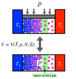
Figure 13: Equivalence of the steady states for different environments. The top figure shows the steady state in the system at the constant pressure $p$, whose volume is $V({\tilde{T}},p,N,\Xi)$. The bottom figure shows the steady state in the constant volume system where the volume $V$ is chosen as $V=V({\tilde{T}},p,N,\Xi)$. The resulting pressure $p({\tilde{T}},V,N,\Xi)$ is equal to $p$.

The fundamental relation (7.23) derived in the previous section is expressed in terms of the state variable $({\tilde{T}},p,N,\Xi)$. As is familiar with thermodynamics, one may consider other fundamental relations. The most familiar one to physicists may be the form using the state variable $({\tilde{T}},V,N,\Xi)$, because this form is directly related to experimental configurations with $({\tilde{T}},V,N,\Xi)$ fixed, instead of $({\tilde{T}},p,N,\Xi)$ fixed in the previous sections. Since the same steady state can be realized when the fixing condition is replaced from $p={\rm const}$ to $V={\rm const}$, there is one-to-one correspondence between $({\tilde{T}},V,N,\Xi)$ and $({\tilde{T}},p,N,\Xi)$. See Fig. 13. In this section, we show thermodynamic relations with volume $V$. In §8.1, we derive the fundamental relation in $({\tilde{T}},V,N,\Xi)$. In §8.2, we express the free energy $F$ by using the saturated pressure $p_{\mathrm{s}}(T)$ for equilibrium systems. Since the value of ${\tilde{T}}$ is not easily controlled in experiments, in §8.3, we formulate $T_{1}$ and $T_{2}$ as functions of ${\tilde{T}}$ and $V$. Below, we fix $N$ without loss of generality and sometimes abbreviate $A({\tilde{T}},N)$ as $A({\tilde{T}})$.

8.1 Fundamental relation

Since ${F}$ and ${G}$ are given as the spatial integral of the local free energies, the uniformity of the pressure leads to

$${G}={F}+pV.$$ (8.1)

Substituting this into (7.22), we have

$$\delta F =-(S+O(\varepsilon^{2}))\delta{\tilde{T}}-(p+O(\varepsilon^{2}))\delta V+(\tilde{\mu}+O(\varepsilon^{2}))\delta N$$

$$\qquad\qquad-\left(\Psi+O(\varepsilon)\right)\delta\Xi+(O(\varepsilon^{2}))N\delta\left(\frac{N^{\mathrm{L}}}{N}\right),$$ (8.2)

where the error of $O(\varepsilon^{2})\delta p$ in (7.22) is regarded as $O(\varepsilon^{2})\delta p({\tilde{T}},V,N,\Xi)$ which results in the error of $O(\varepsilon^{2})\delta V$ besides $O(\varepsilon^{2})\delta{\tilde{T}}$ and so on. The most important thing here is the order estimate of $N\delta(N^{\mathrm{L}}/N)$, which has been estimated as $O(\varepsilon^{-1})$ when $N^{\mathrm{L}}$ is a function of $({\tilde{T}},p,N,\Xi)$. See (7.15). As a function of $({\tilde{T}},V,N,\Xi)$, $N\delta(N^{\mathrm{L}}/N)$ becomes of $O(\varepsilon^{0})$ because the liquid-gas coexistence stably appears at equilibrium ($\varepsilon=0$) in a certain range of $({\tilde{T}},V,N)$ and, therefore, the term is not singular in the limit $\varepsilon\to 0$. Indeed, the second line is estimated as

$$\left(\frac{\partial N^{\mathrm{L}}}{\partial{\tilde{T}}}\right)_{V,\Xi} =\left(\frac{\partial N^{\mathrm{L}}}{\partial{\tilde{T}}}\right)_{p,\Xi}+\left(\frac{\partial N^{\mathrm{L}}}{\partial p}\right)_{p,\Xi}\left(\frac{\partial p}{\partial{\tilde{T}}}\right)_{V,\Xi}$$

$$=-\frac{N}{\Xi}\frac{dT_{\mathrm{c}}}{dp}\left(\frac{dp_{\mathrm{s}}}{d{\tilde{T}}}-\left(\frac{\partial p}{\partial{\tilde{T}}}\right)_{V,\Xi}\right)=O(\varepsilon^{0}),$$ (8.3)

where we have used

$$\left(\frac{\partial p}{\partial{\tilde{T}}}\right)_{V,\Xi}=\frac{dp_{\mathrm{s}}}{d{\tilde{T}}}+O(\varepsilon).$$ (8.4)

Thus, the last term in (8.2) remains to be negligible as $O(\varepsilon^{2})$ term, and we conclude

$$d{F} =-({S}+O(\varepsilon^{2}))d{\tilde{T}}-(p+O(\varepsilon^{2}))dV+(\tilde{\mu}+O(\varepsilon^{2}))dN-\left(\Psi+O(\varepsilon)\right)d\Xi.$$ (8.5)

It should be noted that there are the errors of $O(\varepsilon^{2})$ in contrast to (7.23).

8.2 Free energy for the coexistence phase

In the equilibrium coexistence phase, as shown in Fig. 14, the saturated volumes, $V_{\mathrm{s}}^{\mathrm{L}}(T)$ and $V_{\mathrm{s}}^{\mathrm{G}}(T)$, and the saturated pressure $p_{\mathrm{s}}(T)$ are defined for a given temperature $T$. Even for the coexistence phase in heat conduction, we define the saturated volumes, $V_{\mathrm{s}}^{\mathrm{L}}(\tilde{T},\Xi)$ and $V_{\mathrm{s}}^{\mathrm{G}}(\tilde{T},\Xi)$, at which the liquid and the gas start to coexist. Note that the pressure is not kept constant in $V_{\mathrm{s}}^{\mathrm{L}}({\tilde{T}},\Xi)<V<V_{\mathrm{s}}^{\mathrm{G}}({\tilde{T}},\Xi)$, differently from the equilibrium case.

We first express $V_{\mathrm{s}}^{\mathrm{L}}({\tilde{T}},\Xi)$, $V_{\mathrm{s}}^{\mathrm{G}}({\tilde{T}},\Xi)$ and $p(\tilde{T},V,\Xi)$ in terms of $V_{\mathrm{s}}^{\mathrm{L}}({\tilde{T}})$, $V_{\mathrm{s}}^{\mathrm{G}}({\tilde{T}})$ and $p_{\mathrm{s}}({\tilde{T}})$. Since the steady state satisfies (5.38), we have

$$T_{\mathrm{c}}(p)={\tilde{T}}+\frac{\Xi}{2}\frac{N^{\mathrm{L}}-N^{\mathrm{G}}}{N}+O(\varepsilon^{2}).$$ (8.6)

Solving this in $p$, we obtain

$$p(\tilde{T},V,\Xi)=p_{\mathrm{s}}\left({\tilde{T}}+\frac{\Xi}{2}\frac{N^{\mathrm{L}}-N^{\mathrm{G}}}{N}\right)+O(\varepsilon^{2}).$$ (8.7)

For equilibrium cases, the relations $N^{\mathrm{L}}+N^{\mathrm{G}}=N$ and $N^{\mathrm{L}}V_{\mathrm{s}}^{\mathrm{L}}+N^{\mathrm{G}}V_{\mathrm{s}}^{\mathrm{G}}=NV$ lead to

$$N^{\mathrm{L}}=N\frac{V_{\mathrm{s}}^{\mathrm{G}}({\tilde{T}})-V}{V_{\mathrm{s}}^{\mathrm{G}}({\tilde{T}})-V_{\mathrm{s}}^{\mathrm{L}}({\tilde{T}})},\quad N^{\mathrm{G}}=N\frac{V-V_{\mathrm{s}}^{\mathrm{L}}({\tilde{T}})}{V_{\mathrm{s}}^{\mathrm{G}}({\tilde{T}})-V_{\mathrm{s}}^{\mathrm{L}}({\tilde{T}})}.$$ (8.8)

By using these expressions, we rewrite (8.7) as

$$p({\tilde{T}},V,\Xi)=p_{\mathrm{s}}\left({\tilde{T}}-\Xi\frac{V-V_{\mathrm{m}}({\tilde{T}})}{V_{\mathrm{s}}^{\mathrm{G}}({\tilde{T}})-V_{\mathrm{s}}^{\mathrm{L}}({\tilde{T}})}\right)+O(\varepsilon^{2}),$$ (8.9)

where $V_{\mathrm{m}}({\tilde{T}})=(V_{\mathrm{s}}^{\mathrm{L}}({\tilde{T}})+V_{\mathrm{s}}^{\mathrm{G}}({\tilde{T}}))/2$. Figure 14 shows a $p$-$V$ curve described by (8.9), in which $p({\tilde{T}},V,\Xi)$ is linearly decreasing with $V$ in the range $V_{\mathrm{s}}^{\mathrm{L}}({\tilde{T}},\Xi)<V<V_{\mathrm{s}}^{\mathrm{G}}({\tilde{T}},\Xi)$. Configurations in the phase coexistence are exemplified in Fig. 15. Then, the saturated volumes under heat conduction are expressed as

$$V_{\mathrm{s}}^{\mathrm{L}}({\tilde{T}},\Xi)=V^{\mathrm{L}}\left({\tilde{T}},p_{\mathrm{s}}\left({\tilde{T}}+\frac{\Xi}{2}\right)\right),\quad V_{\mathrm{s}}^{\mathrm{G}}({\tilde{T}},\Xi)=V^{\mathrm{G}}\left({\tilde{T}},p_{\mathrm{s}}\left({\tilde{T}}-\frac{\Xi}{2}\right)\right),$$ (8.10)

where $V=V^{\mathrm{L}}(T,p)$ and $V=V^{\mathrm{G}}(T,p)$ are the equilibrium equation of state for the liquid and the gas, respectively.

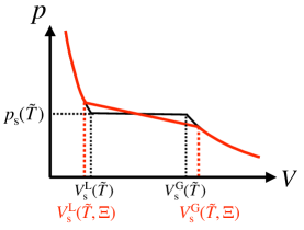
Figure 14: $p$-$V$ curves with ${\tilde{T}}$ fixed for $\Xi=0$ (black line) and for $\Xi\not=0$ (red line). For the equilibrium case $(\Xi=0)$, the pressure is kept constant to be a saturated pressure $p_{\mathrm{s}}({\tilde{T}})$ in the region $V_{\rm s}^{\mathrm{L}}({\tilde{T}})<V<V_{\rm s}^{\mathrm{G}}({\tilde{T}})$, where the liquid and the gas coexist.

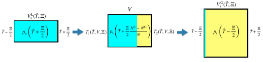
Figure 15: Dependence of the steady state on $V$ for a given ${\tilde{T}}$. The liquid region and the gas region in the container are painted by light blue and yellow, respectively. The pressure changes with increasing $V$ according to (8.9). The temperatures of the two heat baths, $T_{1}$ and $T_{2}$, are controlled to realize fixing $({\tilde{T}},V,\Xi)$ as formulated in (8.33) and (8.34).

Next, we study the free energy $F(\tilde{T},V,\Xi)$. We first consider the free energy difference

$$\Delta^{\rm LG}F\equiv{F}({\tilde{T}},V_{\mathrm{s}}^{\mathrm{G}}({\tilde{T}},\Xi),\Xi)-{F}({\tilde{T}},V_{\mathrm{s}}^{\mathrm{L}}({\tilde{T}},\Xi),\Xi).$$ (8.11)

Since the saturated state is in a single phase, we have

$${F}({\tilde{T}},V_{\mathrm{s}}^{\mathrm{L/G}}({\tilde{T}},\Xi),\Xi)=F^{\mathrm{L/G}}({\tilde{T}},V_{\mathrm{s}}^{\mathrm{L/G}}({\tilde{T}},\Xi))+O(\varepsilon^{2}).$$ (8.12)

We then transform

$$\Delta^{\rm LG}F= F^{\mathrm{G}}({\tilde{T}},V_{\mathrm{s}}^{\mathrm{G}}({\tilde{T}},\Xi))-F^{\mathrm{L}}({\tilde{T}},V_{\mathrm{s}}^{\mathrm{L}}({\tilde{T}},\Xi))+O(\varepsilon^{2})$$

$$= F^{\mathrm{G}}({\tilde{T}},V_{\mathrm{s}}^{\mathrm{G}}({\tilde{T}}))-F^{\mathrm{L}}({\tilde{T}},V_{\mathrm{s}}^{\mathrm{L}}({\tilde{T}}))$$

$$\quad-p_{\mathrm{s}}(\tilde{T})\Xi\left(\left({\frac{\partial V_{\mathrm{s}}^{\mathrm{G}}({\tilde{T}},\Xi)}{\partial\Xi}}\right)_{{\tilde{T}}}-\left({\frac{\partial V_{\mathrm{s}}^{\mathrm{L}}({\tilde{T}},\Xi)}{\partial\Xi}}\right)_{{\tilde{T}}}\right)+O(\varepsilon^{2})$$

$$= -p_{\mathrm{s}}({\tilde{T}})(V_{\mathrm{s}}^{\mathrm{G}}({\tilde{T}},\Xi)-V_{\mathrm{s}}^{\mathrm{L}}({\tilde{T}},\Xi))+O(\varepsilon^{2}),$$ (8.13)

where we have used the Taylor expansion in $\Xi$ to obtain the second line, and substituted the equilibrium relation

$$F^{\mathrm{G}}({\tilde{T}},V_{\mathrm{s}}^{\mathrm{G}}({\tilde{T}}))-F^{\mathrm{L}}({\tilde{T}},V_{\mathrm{s}}^{\mathrm{L}}({\tilde{T}}))=-p_{\mathrm{s}}({\tilde{T}})(V_{\mathrm{s}}^{\mathrm{G}}({\tilde{T}})-V_{\mathrm{s}}^{\mathrm{L}}({\tilde{T}}))$$ (8.14)

to obtain the last line.

Second, from (8.5), we have

$${F}({\tilde{T}},V,\Xi)=F^{\mathrm{L}}({\tilde{T}},V_{\mathrm{s}}^{\mathrm{L}}({\tilde{T}},\Xi))-\int_{V_{\mathrm{s}}^{\mathrm{L}}({\tilde{T}},\Xi)}^{V}P({\tilde{T}},V^{\prime},\Xi)~{}dV^{\prime}.$$ (8.15)

Performing the integration with (8.9), we obtain

$${F}({\tilde{T}},V,\Xi) =F^{\mathrm{L}}({\tilde{T}},V_{\mathrm{s}}^{\mathrm{L}}({\tilde{T}},\Xi))-p_{\mathrm{s}}({\tilde{T}})(V-V_{\mathrm{s}}^{\mathrm{L}}({\tilde{T}},\Xi))-B\Xi$$ (8.16)

with

$$B=\frac{dp_{\mathrm{s}}({\tilde{T}})}{d{\tilde{T}}}\frac{V_{\mathrm{s}}^{\mathrm{G}}({\tilde{T}})-V_{\mathrm{s}}^{\mathrm{L}}({\tilde{T}})}{2}\left[\frac{1}{4}-\left(\frac{V-V_{\mathrm{m}}({\tilde{T}})}{V_{\mathrm{s}}^{\mathrm{G}}({\tilde{T}})-V_{\mathrm{s}}^{\mathrm{L}}({\tilde{T}})}\right)^{2}\right]+O(\varepsilon).$$ (8.17)

Here, by using (8.8), we can confirm

$$\frac{N^{\mathrm{L}}N^{\mathrm{G}}}{N^{2}}=\frac{1}{4}-\left(\frac{V-V_{\mathrm{m}}({\tilde{T}})}{V_{\mathrm{s}}^{\mathrm{G}}({\tilde{T}})-V_{\mathrm{s}}^{\mathrm{L}}({\tilde{T}})}\right)^{2}.$$ (8.18)

Combining it with the Clausius-Clapeyron relation

$$\frac{dp_{\mathrm{s}}({\tilde{T}})}{d{\tilde{T}}}({V_{\mathrm{s}}^{\mathrm{G}}({\tilde{T}})-V_{\mathrm{s}}^{\mathrm{L}}({\tilde{T}})})=N\frac{\hat{q}}{{\tilde{T}}},$$ (8.19)

we derive

$$B=\Psi,$$ (8.20)

where $\Psi$ was introduced in (7.18). Summarizing these, we schematically draw the graph ${F}$ in Fig. 16. For equilibrium cases, the free energy of the liquid-gas coexistence phase is expressed as a common tangent at $V_{\mathrm{s}}^{\mathrm{L}}({\tilde{T}})$ and $V_{\mathrm{s}}^{\mathrm{G}}({\tilde{T}})$ as shown in Fig. 16(a). For heat conduction cases, the free energy of the coexistence phase is expressed as a common tangential quadratic curve at $V_{\mathrm{s}}^{\mathrm{L}}({\tilde{T}},\Xi)$ and $V_{\mathrm{s}}^{\mathrm{G}}({\tilde{T}},\Xi)$ as shown in Fig 16(b), and therefore $F$ keeps the convexity on $V$.

Since the convexity of $F$ is concluded, the Gibbs free energy $G$ is expressed as the Legendre transform of $F$:

$$G({\tilde{T}},p,\Xi)=\min_{V}[F({\tilde{T}},V,\Xi)+pV].$$ (8.21)

The graph $F$ in Fig. 16(b) yields the graph $G$ in Fig. 17(b), while it contains an error of $O(\varepsilon^{2})$ as well as $F$ formulated explicitly in (8.16). The liquid-gas coexistence states are expressed as a common tangential quadratic curve to the graph $G$ at $p_{\mathrm{s}}({\tilde{T}}+\Xi/2)$ and $p_{\mathrm{s}}({\tilde{T}}-\Xi/2)$.

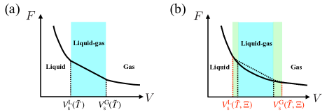
Figure 16: Schematic figure of the global Helmholtz free energy $F$ with ${\tilde{T}}$ fixed when ${\tilde{T}}$ is less than the critical temperature. (a) Equilibrium cases. $F$ is a linear function in the light blue area, $V_{\mathrm{s}}^{\mathrm{L}}({\tilde{T}})<V<V_{\mathrm{s}}^{\mathrm{G}}({\tilde{T}})$, where the system shows the liquid-gas coexistence. (b) Heat conduction cases with $\Xi>0$. The solid line becomes a quadratic curve in $V_{\mathrm{s}}^{\mathrm{L}}({\tilde{T}},\Xi)<V<V_{\mathrm{s}}^{\mathrm{G}}({\tilde{T}},\Xi)$ painted by light blue and green, where the system shows the liquid-gas coexistence. $F$ is smooth at $V=V_{\mathrm{s}}^{\mathrm{L/G}}({\tilde{T}},\Xi)$. The dotted line represents $F$ at equilibrium in (a). The solid and dotted lines are the same in $V<V_{\mathrm{s}}^{\mathrm{L}}({\tilde{T}},\Xi)$ and $V>V_{\mathrm{s}}^{\mathrm{G}}({\tilde{T}},\Xi)$.

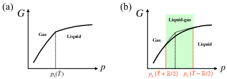
Figure 17: Schematic figure of the global Gibbs free energy $G$ with ${\tilde{T}}$ fixed, where ${\tilde{T}}$ is less than the critical temperature. (a) Equilibrium cases. $G$ exhibits the first order transition at $p=p_{\mathrm{s}}({\tilde{T}})$, at which $G$ is continuous but not smooth. (b) Heat conduction cases with $\Xi>0$. $G$ contains a quadratic curve in $p_{\mathrm{s}}({\tilde{T}}+\Xi/2)<p<p_{\mathrm{s}}({\tilde{T}}-\Xi/2)$, in which the system shows the liquid-gas coexistence (solid line). $G$ is smooth at $p=p_{\mathrm{s}}({\tilde{T}}\pm\Xi/2)$. The dotted line represents $G$ at equilibrium in (a). The solid and dotted lines are the same in $p<p_{\mathrm{s}}^{\mathrm{L}}({\tilde{T}}+\Xi/2)$ and $p>p_{\mathrm{s}}^{\mathrm{G}}({\tilde{T}}-\Xi/2)$.

8.3 $T_{1}$, $T_{2}$ and $\theta$ as functions of $({\tilde{T}},V,N,\Xi)$

We have studied the dependence of the steady states on $V$ for $({\tilde{T}},\Xi)$ fixed. However, when we fix values of $T_{1}$ and $T_{2}$, the change of $V$ yields the change of ${\tilde{T}}$. Here we propose a protocol to control $T_{1}$ and $T_{2}$, by which ${\tilde{T}}$ is fixed when changing $V$. In other words, we derive $T_{1}$ and $T_{2}$ as functions of $({\tilde{T}},V,N,\Xi)$. We also give the interface temperature $\theta$ and its deviation from $T_{\mathrm{c}}$ as functions of $({\tilde{T}},V,N,\Xi)$.

In (6.8), $T_{\mathrm{m}}$ is expressed in terms of $T_{\mathrm{c}}(p)$, $\Xi$, $u$, $v$, and $\zeta$, where the value of $u$ and $v$ are determined for each $p$. For the coexistence phase in heat conduction, the pressure is determined as (8.9) and can be replaced by $p_{\mathrm{s}}({\tilde{T}})$ for the argument of $u$ and $v$. We thus represent $u=u(p_{\mathrm{s}}({\tilde{T}}))$ and $v=v(p_{\mathrm{s}}({\tilde{T}}))$, and simply write $u({\tilde{T}})$ and $v({\tilde{T}})$. Then, we rewrite (6.8) as

$$T_{\mathrm{m}}=T_{\mathrm{c}}(p({\tilde{T}},V,\Xi))-\frac{\Xi}{2}\frac{u\zeta^{2}-v(1-\zeta)^{2}}{[u\zeta+(1-\zeta)][\zeta+v(1-\zeta)]}+O(\varepsilon^{2})$$ (8.22)

with

$$u({\tilde{T}})=\frac{V_{\mathrm{s}}^{\mathrm{G}}({\tilde{T}})}{V_{\mathrm{s}}^{\mathrm{L}}({\tilde{T}})},\qquad v({\tilde{T}})=\frac{\kappa_{\mathrm{c}}^{\mathrm{L}}({\tilde{T}})}{\kappa_{\mathrm{c}}^{\mathrm{G}}({\tilde{T}})}.$$ (8.23)

Furthermore, from

$$\zeta=\frac{N^{\mathrm{L}}}{N}\frac{V_{\mathrm{s}}^{\mathrm{L}}}{V},$$ (8.24)

and $N^{\mathrm{L}}V_{\mathrm{s}}^{\mathrm{L}}+N^{\mathrm{G}}V_{\mathrm{s}}^{\mathrm{G}}=NV$ at equilibrium, we obtain

$$\zeta =\frac{(V_{\mathrm{s}}^{\mathrm{G}}({\tilde{T}})-V)V_{\mathrm{s}}^{\mathrm{L}}({\tilde{T}})}{(V_{\mathrm{s}}^{\mathrm{G}}({\tilde{T}})-V_{\mathrm{s}}^{\mathrm{L}}({\tilde{T}}))V}+O(\varepsilon).$$ (8.25)

These expressions of $u$, $v$ and $\zeta$ lead to

$$\frac{1}{u\zeta+(1-\zeta)}=\frac{V}{V_{\mathrm{s}}^{\mathrm{G}}},$$ (8.26)

$$\frac{1}{\zeta+v(1-\zeta)}=\frac{V(V_{\mathrm{s}}^{\mathrm{G}}-V_{\mathrm{s}}^{\mathrm{L}})}{V_{\mathrm{s}}^{\mathrm{L}}(V_{\mathrm{s}}^{\mathrm{G}}-V)+vV_{\mathrm{s}}^{\mathrm{G}}(V-V_{\mathrm{s}}^{\mathrm{L}})},$$ (8.27)

$$u\zeta^{2}-v(1-\zeta)^{2}=\frac{V_{\mathrm{s}}^{\mathrm{G}}[V_{\mathrm{s}}^{\mathrm{L}}(V_{\mathrm{s}}^{\mathrm{G}}-V)^{2}-vV_{\mathrm{s}}^{\mathrm{G}}(V-V_{\mathrm{s}}^{\mathrm{L}})^{2}]}{V^{2}(V_{\mathrm{s}}^{\mathrm{G}}-V_{\mathrm{s}}^{\mathrm{L}})^{2}},$$ (8.28)

with which (8.22) is rewritten as

$$T_{\mathrm{m}}=T_{\mathrm{c}}(p)-\frac{\Xi}{2}\frac{1}{V_{\mathrm{s}}^{\mathrm{G}}-V_{\mathrm{s}}^{\mathrm{L}}}\frac{V_{\mathrm{s}}^{\mathrm{L}}(V_{\mathrm{s}}^{\mathrm{G}}-V)^{2}-vV_{\mathrm{s}}^{\mathrm{G}}(V-V_{\mathrm{s}}^{\mathrm{L}})^{2}}{V_{\mathrm{s}}^{\mathrm{L}}(V_{\mathrm{s}}^{\mathrm{G}}-V)+vV_{\mathrm{s}}^{\mathrm{G}}(V-V_{\mathrm{s}}^{\mathrm{L}})}.$$ (8.29)

Here, let us recall that $T_{\mathrm{c}}(p)={\tilde{T}}-\Xi r$ defined in (5.43) and that

$$r=\frac{V-V_{\mathrm{m}}({\tilde{T}})}{V_{\mathrm{s}}^{\mathrm{G}}({\tilde{T}})-V_{\mathrm{s}}^{\mathrm{L}}({\tilde{T}})}+O(\varepsilon)$$ (8.30)

as used in (8.9). Substituting this formula into (8.29) and noting

$$V-V_{\mathrm{m}}({\tilde{T}})=\frac{V-V_{\mathrm{s}}^{\mathrm{G}}({\tilde{T}})}{2}+\frac{V-V_{\mathrm{s}}^{\mathrm{L}}({\tilde{T}})}{2},$$ (8.31)

we finally arrive at

$$T_{\mathrm{m}}({\tilde{T}},V,\Xi)={\tilde{T}}-\frac{\Xi}{2}\frac{(V-V_{\mathrm{s}}^{\mathrm{L}})(V_{\mathrm{s}}^{\mathrm{G}}-V)(V_{\mathrm{s}}^{\mathrm{L}}-vV_{\mathrm{s}}^{\mathrm{G}})}{(V_{\mathrm{s}}^{\mathrm{G}}-V_{\mathrm{s}}^{\mathrm{L}})(V_{\mathrm{s}}^{\mathrm{L}}(V_{\mathrm{s}}^{\mathrm{G}}-V)+vV_{\mathrm{s}}^{\mathrm{G}}(V-V_{\mathrm{s}}^{\mathrm{L}}))}+O(\varepsilon^{2}).$$ (8.32)

Since $T_{\mathrm{m}}=(T_{1}+T_{2})/2$ and $\Xi=T_{2}-T_{1}$, we obtain

$$T_{1}({\tilde{T}},V,\Xi)={\tilde{T}}-\frac{\Xi}{2}-\frac{\Xi}{2}\frac{(V-V_{\mathrm{s}}^{\mathrm{L}})(V_{\mathrm{s}}^{\mathrm{G}}-V)(V_{\mathrm{s}}^{\mathrm{L}}-vV_{\mathrm{s}}^{\mathrm{G}})}{(V_{\mathrm{s}}^{\mathrm{G}}-V_{\mathrm{s}}^{\mathrm{L}})(V_{\mathrm{s}}^{\mathrm{L}}(V_{\mathrm{s}}^{\mathrm{G}}-V)+vV_{\mathrm{s}}^{\mathrm{G}}(V-V_{\mathrm{s}}^{\mathrm{L}}))}+O(\varepsilon^{2}),$$ (8.33)

$$T_{2}({\tilde{T}},V,\Xi)={\tilde{T}}+\frac{\Xi}{2}-\frac{\Xi}{2}\frac{(V-V_{\mathrm{s}}^{\mathrm{L}})(V_{\mathrm{s}}^{\mathrm{G}}-V)(V_{\mathrm{s}}^{\mathrm{L}}-vV_{\mathrm{s}}^{\mathrm{G}})}{(V_{\mathrm{s}}^{\mathrm{G}}-V_{\mathrm{s}}^{\mathrm{L}})(V_{\mathrm{s}}^{\mathrm{L}}(V_{\mathrm{s}}^{\mathrm{G}}-V)+vV_{\mathrm{s}}^{\mathrm{G}}(V-V_{\mathrm{s}}^{\mathrm{L}}))}+O(\varepsilon^{2}).$$ (8.34)

These formulas inform how to operate $T_{1}$ and $T_{2}$ in order to fix the global temperature ${\tilde{T}}$ when changing $V$ and $\Xi$.

Substituting the temperature relation (5.47) into (8.29), we obtain the interface temperature as

$$\theta({\tilde{T}},V,\Xi)={\tilde{T}}+\frac{\Xi}{2}\frac{1}{V_{\mathrm{s}}^{\mathrm{G}}-V_{\mathrm{s}}^{\mathrm{L}}}\frac{V_{\mathrm{s}}^{\mathrm{L}}(V_{\mathrm{s}}^{\mathrm{G}}-V)^{2}-vV_{\mathrm{s}}^{\mathrm{G}}(V-V_{\mathrm{s}}^{\mathrm{L}})^{2}}{V_{\mathrm{s}}^{\mathrm{L}}(V_{\mathrm{s}}^{\mathrm{G}}-V)+vV_{\mathrm{s}}^{\mathrm{G}}(V-V_{\mathrm{s}}^{\mathrm{L}})}.$$ (8.35)

Similarly, (8.32) and (5.47) lead to the deviation from the transition temperature,

$$\theta({\tilde{T}},V,\Xi)-T_{\mathrm{c}}(p({\tilde{T}},V,\Xi))$$

$$\qquad=\frac{\Xi}{2}\frac{(V-V_{\mathrm{s}}^{\mathrm{L}})(V_{\mathrm{s}}^{\mathrm{G}}-V)(V_{\mathrm{s}}^{\mathrm{L}}-vV_{\mathrm{s}}^{\mathrm{G}})}{(V_{\mathrm{s}}^{\mathrm{G}}-V_{\mathrm{s}}^{\mathrm{L}})(V_{\mathrm{s}}^{\mathrm{L}}(V_{\mathrm{s}}^{\mathrm{G}}-V)+vV_{\mathrm{s}}^{\mathrm{G}}(V-V_{\mathrm{s}}^{\mathrm{L}}))}+O(\varepsilon^{2}).$$ (8.36)

9 Other assumptions leading to the results of the variational principle

To this point, it has been assumed that the steady states are determined by the variational principle proposed in §5. In this section, we introduce other assumptions from which the result of the variational principle is obtained. First, in §9.1, we formulate the variational principle for the constant volume systems and show that its solution is equivalent to the previous one (5.38). In §9.2, we start with the fundamental relation of thermodynamics without assuming the variational principle. We then derive the result of the variational principle. In §9.3, we notice a singularity relation which is a simple assumption for the singularity in the limit $\varepsilon\to 0$. We confirm that this is equivalent to the result of the variational principle. Finally, in §9.4 we argue some scaling behavior of the system which also leads to the result of the variational principle.

9.1 Variational principle for constant volume systems

In this subsection, we study constant volume systems, where the steady state is characterized by $({\tilde{T}},V,\Xi,N)$. As shown in Fig. 13, this steady state is equivalent to the steady state of the system at the constant pressure $p^{\mathrm{ex}}$ when the value of $p^{\mathrm{ex}}$ is chosen as the pressure $p({\tilde{T}},V,N,\Xi)$. We assume the mechanical balance everywhere. That is,

$$p(x)=p(x^{\prime})$$ (9.1)

for any $x$ and $x^{\prime}$ in $[0,L_{x}]$, where $p(x)=p(T(x),\rho(x))$. This condition determines $V^{\mathrm{L}}$ and $V^{\mathrm{G}}=V-V^{\mathrm{L}}$ when $N^{\mathrm{L}}$ and $N^{\mathrm{G}}=N-N^{\mathrm{L}}$ are determined. The problem is then to determine $N^{\mathrm{L}}$. After briefly reviewing the corresponding variational principle for equilibrium cases, we propose the variational principle for heat conduction systems and determine the value of $N^{\mathrm{L}}$.

9.1.1 Equilibrium systems

We define the variational function as

$${\cal F}({\cal N}^{\mathrm{L}};T,V,N) =F^{\mathrm{L}}(T,V^{\mathrm{L}},{\cal N}^{\mathrm{L}})+F^{\mathrm{G}}(T,V-V^{\mathrm{L}},N-{\cal N}^{\mathrm{L}}),$$ (9.2)

in which $F^{\mathrm{L/G}}(T,V,N)$ is the Helmholtz free energy of the liquid (gas). $V^{\mathrm{L}}$ and $V^{\mathrm{G}}$ are determined by

$$p(T,{\cal N}^{\mathrm{L}}/V^{\mathrm{L}})=p(T,(N-{\cal N}^{\mathrm{L}})/V^{\mathrm{G}}),$$ (9.3)

and $V^{\mathrm{L}}+V^{\mathrm{G}}=V$. Then, the variational principle for determining ${\cal N}^{\mathrm{L}}$ is

$$\left.\frac{\partial{\cal F}({\cal N}^{\mathrm{L}};T,V,N)}{\partial{\cal N}^{\mathrm{L}}}\right|_{{\cal N}^{\mathrm{L}}=N^{\mathrm{L}}}=0,\qquad\left.\frac{\partial^{2}{\cal F}({\cal N}^{\mathrm{L}};T,V,N)}{\partial({\cal N}^{\mathrm{L}})^{2}}\right|_{{\cal N}^{\mathrm{L}}=N^{\mathrm{L}}}>0,$$ (9.4)

which is equivalent to the equality of the chemical potential.

9.1.2 Heat conduction systems

Let us consider a variational principle for the heat conduction systems characterized by $({\tilde{T}},V,N,\Xi)$. We assume that the steady state with a liquid-gas interface is determined by the variational function

$${\cal F}({\cal N}^{\mathrm{L}};{\tilde{T}},V,N,\Xi) \equiv L_{y}L_{z}\int_{0}^{L_{x}}dx~{}~{}f(T(x),\rho(x))$$

$$=F^{\mathrm{L}}({\tilde{T}}^{\mathrm{L}},V^{\mathrm{L}},{\cal N}^{\mathrm{L}})+F^{\mathrm{G}}({\tilde{T}}^{\mathrm{G}},V-V^{\mathrm{L}},N-{\cal N}^{\mathrm{L}})+O(\varepsilon^{2}),$$ (9.5)

where we have used a similar formula as (7.3) with (7.4) and (7.5) to obtain the second line. As we formulated in §4, thermodynamic quantities are expressed as a function of ${\cal N}^{\mathrm{L}}$ such that ${\tilde{T}}^{\mathrm{L/G}}={\tilde{T}}^{\mathrm{L/G}}({\cal N}^{\mathrm{L}};{\tilde{T}},V,N,\Xi)$. The variation of ${\cal F}$ is then written as

$$\delta{\cal F}=\delta F^{\mathrm{L}}+\delta F^{\mathrm{G}}.$$ (9.6)

Remembering that the relation (5.20) holds in each region, we have

$$\delta F^{\mathrm{L/G}}=-S^{\mathrm{L/G}}\delta{\tilde{T}}^{\mathrm{L/G}}-p\delta V^{\mathrm{L/G}}+\tilde{\mu}^{\mathrm{L/G}}\delta{\cal N}^{\mathrm{L/G}}.$$ (9.7)

Substituting $\delta{\cal N}^{\mathrm{G}}=-\delta{\cal N}^{\mathrm{L}}$, $\delta V^{\mathrm{L}}+\delta V^{\mathrm{G}}=0$ and (5.28) into (9.7), we rewrite (9.6) as

$$\delta{\cal F}=(\mu^{\mathrm{L}}(T^{\rm s},p)-\mu^{\mathrm{G}}(T^{\rm s},p)+O(\varepsilon^{2}))\delta{\cal N}^{\mathrm{L}},$$ (9.8)

where $T^{\rm s}$ is given in (5.32). Then, the variational principle

$$\left.\frac{\partial{\cal F}({\cal N}^{\mathrm{L}};{\tilde{T}},V,N,\Xi)}{\partial{\cal N}^{\mathrm{L}}}\right|_{{\cal N}^{\mathrm{L}}=N^{\mathrm{L}}}=0,\qquad\left.\frac{\partial^{2}{\cal F}({\cal N}^{\mathrm{L}};{\tilde{T}},V,N,\Xi)}{\partial({\cal N}^{\mathrm{L}})^{2}}\right|_{{\cal N}^{\mathrm{L}}=N^{\mathrm{L}}}>0$$ (9.9)

determines ${\cal N}^{\mathrm{L}}$ as that satisfying

$$\mu^{\mathrm{L}}(T^{\rm s},p)=\mu^{\mathrm{G}}(T^{\rm s},p)+O(\varepsilon^{2}).$$ (9.10)

This is equivalent to (5.36) so that (9.10) leads to (5.38). Therefore, the variational principle for the constant volume system is equivalent to that for the system at constant pressure.

9.2 Thermodynamic relation

In this subsection, we do not assume any variational principles, but assume the fundamental relation of thermodynamics

$$dF=-Sd{\tilde{T}}-pdV+\tilde{\mu}dN-\Psi d\Xi$$ (9.11)

for the liquid-gas coexistence phase in the linear response regime.

First of all, it should be noted that (7.10), (7.11), (7.12) and (7.13) hold regardless of the variational principle. Then, we have

$$\delta{A}= \left(N^{\mathrm{L}}\left(\frac{\partial\hat{a}^{\mathrm{L}}}{\partial{\tilde{T}}^{\mathrm{L}}}\right)_{p}+N^{\mathrm{G}}\left(\frac{\partial\hat{a}^{\mathrm{G}}}{\partial{\tilde{T}}^{\mathrm{G}}}\right)_{p}+O(\varepsilon^{2})\right)\delta{\tilde{T}}$$

$$+\left(N^{\mathrm{L}}\left(\frac{\partial\hat{a}^{\mathrm{L}}}{\partial p}\right)_{{\tilde{T}}^{\mathrm{L}}}+N^{\mathrm{G}}\left(\frac{\partial\hat{a}^{\mathrm{G}}}{\partial p}\right)_{{\tilde{T}}^{\mathrm{G}}}+O(\varepsilon^{2})\right)\delta p$$

$$+\left(\frac{N^{\mathrm{L}}}{N}\hat{a}^{\mathrm{L}}+\frac{N^{\mathrm{G}}}{N}\hat{a}^{\mathrm{G}}+O(\varepsilon^{2})\right)\delta N$$

$$-\frac{N^{\mathrm{L}}N^{\mathrm{G}}}{2N}\left(\left(\frac{\partial\hat{a}^{\mathrm{L}}}{\partial{\tilde{T}}^{\mathrm{L}}}\right)_{p}-\left(\frac{\partial\hat{a}^{\mathrm{G}}}{\partial{\tilde{T}}^{\mathrm{G}}}\right)_{p}+O(\varepsilon)\right)\delta\Xi$$

$$+\left(\hat{a}^{\mathrm{L}}(T_{\mathrm{m}}-{\tilde{T}}-\theta,p)-\hat{a}^{\mathrm{G}}(T_{\mathrm{m}}-{\tilde{T}}-\theta,p)+O(\varepsilon^{2})\right)N\delta\left(\frac{N^{\mathrm{L}}}{N}\right)$$ (9.12)

instead of (7.14). Letting $A=G$ and $\hat{a}=\tilde{\mu}$, and using $G=F+pV$, we obtain

$$\delta F =-(S+O(\varepsilon^{2}))\delta{\tilde{T}}-(p+O(\varepsilon^{2}))\delta V+(\tilde{\mu}+O(\varepsilon^{2}))\delta N$$

$$\qquad\qquad-\left(\Psi+O(\varepsilon)\right)\delta\Xi+(D+O(\varepsilon^{2}))N\delta\left(\frac{N^{\mathrm{L}}}{N}\right),$$ (9.13)

where

$$D\equiv\mu^{\rm L}(T_{\mathrm{m}}-{\tilde{T}}-\theta,p)-\mu^{\rm G}(T_{\mathrm{m}}-{\tilde{T}}-\theta,p).$$ (9.14)

Since $N\delta(N^{\mathrm{L}}/{N})=O(\varepsilon^{0})$, the assumption (9.11) leads to

$$D=0.$$ (9.15)

This means the temperature relation (5.47). As shown in §5.3, (5.47) leads to (5.38) so that the thermodynamic relation is equivalent to the variational principle.

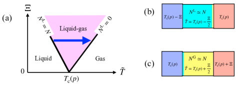
Figure 18: (a) Phase diagram for a given $p$. The line depicted as $N^{\mathrm{L}}=N$ corresponds to ${\tilde{T}}=T_{\mathrm{c}}(p)-{\Xi}/{2}$ from (9.22), at which the gas region starts to appear as shown in (b). Similarly, the line as $N^{\mathrm{L}}=0$, i.e., $N^{\mathrm{G}}=N$, is ${\tilde{T}}=T_{\mathrm{c}}(p)-\frac{\Xi}{2}$, at which the liquid region disappears as shown in (c).

9.3 Singularity relation

We here consider a protocol to shift the liquid-gas interface from $X=L_{x}$ to $X=0$ with fixing $\Xi$ and $p$. This protocol is obtained by varying $(T_{1},T_{2})$ as

$$\left(T_{\mathrm{c}}(p)-\Xi,T_{\mathrm{c}}(p)\right)\quad\rightarrow\quad\left(T_{\mathrm{c}}(p),T_{\mathrm{c}}(p)+\Xi\right),$$ (9.16)

as shown in Figs. 18(b) and (c), where $({\tilde{T}},N^{\mathrm{L}})$ is changed as

$$\left(T_{\mathrm{c}}(p)-\frac{\Xi}{2},N\right)\quad\rightarrow\quad\left(T_{\mathrm{c}}(p)+\frac{\Xi}{2},0\right).$$ (9.17)

On the phase diagram of $({\tilde{T}},\Xi)$ for a given $p$, the change occurs along the line displayed by the arrow in Fig. 18(a) when $\Xi$ is sufficiently small. Therefore, it is natural to assume that

$$\left(\frac{\partial{\tilde{T}}}{\partial N^{\mathrm{L}}}\right)_{p,\Xi} =-\frac{\Xi}{N}+O(\varepsilon^{2})$$ (9.18)

for sufficiently small $\Xi$. This differential equation (9.18) is written as

$$\left(\frac{\partial N^{\mathrm{L}}}{\partial{\tilde{T}}}\right)_{p,\Xi}=-\frac{N}{\Xi}+O(\varepsilon^{0}),$$ (9.19)

which we call a singularity relation. Solving (9.18) with the boundary conditions

$${\tilde{T}}(N^{\mathrm{L}}=N-0,p,\Xi)=T_{\mathrm{c}}(p)-\frac{\Xi}{2}+O(\varepsilon^{2})$$ (9.20)

in Fig. 18(b) and

$${\tilde{T}}(N^{\mathrm{L}}=+0,p,\Xi)=T_{\mathrm{c}}(p)+\frac{\Xi}{2}+O(\varepsilon^{2})$$ (9.21)

in Fig. 18(c), we obtain

$${\tilde{T}} =T_{\mathrm{c}}(p)+\frac{\Xi}{2}\frac{N^{\mathrm{G}}-N^{\mathrm{L}}}{N}+O(\varepsilon^{2}),$$ (9.22)

which is the same form as the result of the variational principle (5.38).

The relation (9.19) indicates

$$\left|\left(\frac{\partial N^{\mathrm{L}}}{\partial{\tilde{T}}}\right)_{P,\Xi}\right|\xrightarrow{\Xi\rightarrow 0}\infty,$$ (9.23)

which corresponds to an expression of the singularity associated with the first-order transition for equilibrium cases. This singularity is consistent with the discontinuous change of $N^{\mathrm{L}}$ at $T=T_{\mathrm{c}}(p)$. It should be noted that (9.23) is connected to the singularity of constant pressure heat capacity $C_{p}$ and compressibility $\alpha_{T}$ as shown in §7.5.

9.4 Scaling relation

We characterize the coexistence phase by $(p^{\mathrm{ex}},N^{\mathrm{L}},\Xi,N)$. As examples, we write

$${\tilde{T}}^{\mathrm{L}} ={\tilde{T}}^{\mathrm{L}}(p^{\mathrm{ex}},N^{\mathrm{L}},\Xi,N),$$ (9.24)

$${\tilde{T}}^{\mathrm{G}} ={\tilde{T}}^{\mathrm{G}}(p^{\mathrm{ex}},N^{\mathrm{L}},\Xi,N).$$ (9.25)

From the homogeneity in the direction perpendicular to $x$, ${\tilde{T}}^{\mathrm{L}}$ and ${\tilde{T}}^{\mathrm{G}}$ are invariant for $(p^{\mathrm{ex}},N^{\mathrm{L}},\Xi,N)\to(p^{\mathrm{ex}},\lambda N^{\mathrm{L}},\Xi,\lambda N)$. We thus write

$${\tilde{T}}^{\mathrm{L}} = {\tilde{T}}^{\mathrm{L}}(p^{\mathrm{ex}},s,\Xi),$$ (9.26)

$${\tilde{T}}^{\mathrm{G}} = {\tilde{T}}^{\mathrm{G}}(p^{\mathrm{ex}},s,\Xi),$$ (9.27)

where

$$s=\frac{N^{\mathrm{L}}}{N}.$$ (9.28)

By noting ${\tilde{T}}^{\mathrm{G}}-{\tilde{T}}^{\mathrm{L}}=\Xi/2$, we express ${\tilde{T}}^{\mathrm{L}}$ and ${\tilde{T}}^{\mathrm{G}}$ as

$${\tilde{T}}^{\mathrm{L}} = T_{\mathrm{c}}(p^{\mathrm{ex}})-\tau(p^{\mathrm{ex}},s)\frac{\Xi}{2}+O(\varepsilon^{2}),$$ (9.29)

$${\tilde{T}}^{\mathrm{G}} = T_{\mathrm{c}}(p^{\mathrm{ex}})+(1-\tau(p^{\mathrm{ex}},s))\frac{\Xi}{2}+O(\varepsilon^{2}).$$ (9.30)

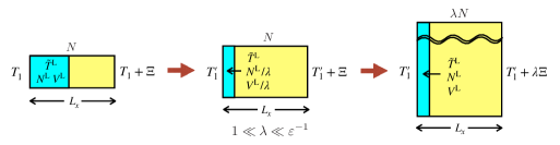
Figure 19: Scaling to extend the gas region with keeping the state in the liquid region and the horizontal length $L_{x}$. In order to fix ${\tilde{T}}^{\mathrm{L}}$, the temperature of the left heat bath is changed from $T_{1}$ to $T_{1}^{\prime}$.

Now, we attempt to extend the gas region while keeping the thermodynamic state in the liquid region. See Fig. 19. First, we increase $\Xi$ as $\Xi\to\lambda\Xi$ with ${\tilde{T}}^{\mathrm{L}}$ fixed, where we take $\lambda\ll\varepsilon^{-1}$ such that the system is still in the linear response regime. We estimate the $\lambda$ dependence of quantities in this asymptotic regime. First, the heat flux is proportional to $\lambda$ as a common value to the liquid and the gas region. Since ${\tilde{T}}^{\mathrm{L}}$ is fixed, it is plausible that the temperature difference in the liquid region remains to be $O(\lambda^{0})$, and then this leads that the horizontal length of the liquid region is proportional to $1/\lambda$. On the other hand, in the gas region, the temperature difference is proportional to $\lambda$ and the horizontal length is $L_{x}$ in the leading order estimate. Thus, the total volume saturates at the finite value with which the whole system is occupied by the gas with the temperature less than $T_{\mathrm{c}}(p^{\mathrm{ex}})+\lambda\Xi$. From these, we find that the volume of the liquid region is proportional to $1/\lambda$. Although its proportional coefficient is not determined in the asymptotic region, we assume the scaling relation that the volume of the liquid is $V^{\mathrm{L}}/\lambda$ as it is consistent with the case $\lambda=1$. Since $p^{\mathrm{ex}}$ and ${\tilde{T}}^{\mathrm{L}}$ is fixed in this operation, the density of the liquid is also fixed. Thus, the particle number of the liquid becomes $N^{\mathrm{L}}/\lambda$. Next, we increase $N$ as $N\to\lambda N$. Then, we have $N^{\mathrm{L}}/\lambda\to N^{\mathrm{L}}$ and $V^{\mathrm{L}}/\lambda\to V^{\mathrm{L}}$. That is, for a series of processes

$$(p^{\mathrm{ex}},N^{\mathrm{L}},\Xi,N)\to(p^{\mathrm{ex}},N^{\mathrm{L}},\lambda\Xi,\lambda N),$$ (9.31)

we have

$${\tilde{T}}^{\mathrm{L}}(p^{\mathrm{ex}},N^{\mathrm{L}},\lambda\Xi,\lambda N)={\tilde{T}}^{\mathrm{L}}(p^{\mathrm{ex}},N^{\mathrm{L}},\Xi,N).$$ (9.32)

Since this condition cannot be concluded from the local equilibrium thermodynamics, we impose (9.32) as a requirement for the steady state.

By using (9.29) for (9.32), we have

$$\tau\left(p^{\mathrm{ex}},\frac{s}{\lambda}\right)\lambda=\tau(p^{\mathrm{ex}},s)$$ (9.33)

for $1\ll\lambda\ll\varepsilon^{-1}$. Expanding

$$\tau(p^{\mathrm{ex}},s)=a_{0}+a_{1}s+a_{2}s^{2}+O(s^{3}),$$ (9.34)

and substituting it to (9.33), we obtain

$$a_{0}(\lambda-1)+a_{2}s^{2}(\lambda^{-1}-1)+\cdots=0$$ (9.35)

for $1\ll\lambda\ll\varepsilon^{-1}$. This gives $a_{0}=a_{2}=a_{n}=0$ for $n\geq 3$. Thus,

$$\tau\left(p^{\mathrm{ex}},s\right)=a_{1}s,$$ (9.36)

which restricts the $s$ dependence of $\tau$.

Next, we extend the liquid region while keeping the gas region. In this case, we consider the transformation $(\Xi,N)\to(\lambda\Xi,\lambda N)$, while fixing $({\tilde{T}}^{\mathrm{G}},N^{\mathrm{G}})$. From (9.30), we have

$$\left[1-\tau\left(p^{\mathrm{ex}},1-\frac{N^{\mathrm{G}}}{\lambda N}\right)\right]\lambda=1-\tau\left(p^{\mathrm{ex}},1-\frac{N^{\mathrm{G}}}{N}\right).$$ (9.37)

Expanding

$$\tau(p^{\mathrm{ex}},1-u)=b_{0}+b_{1}u+O(u^{2})$$ (9.38)

in the limit $u\to 0$, we obtain $b_{0}=1$ and $b_{n}=0$ for $n\geq 2$. This leads to

$$b_{1}\left(1-s\right)=1-\tau\left(p^{\mathrm{ex}},s\right).$$ (9.39)

By combining (9.36) and (9.39), we obtain

$$b_{1}(1-s)=1-a_{1}s.$$ (9.40)

Since this holds for any $s$, we obtain $b_{1}=a_{1}=1$. By substituting (9.36) with $a_{1}=1$ into (9.29), we have arrived at

$${\tilde{T}}^{\mathrm{L}}=T_{\mathrm{c}}(p^{\mathrm{ex}})-\frac{\Xi}{2}\frac{N^{\mathrm{L}}}{N}+O(\varepsilon^{2}).$$ (9.41)

Substituting (5.23) into this relation, we obtain the solution (5.38) of the variational principle.

10 Generalization for single phase systems

In previous sections, global thermodynamics has been developed for systems in a rectangular container as shown in Fig. 2. In this section, we consider an arbitrarily shaped container ${\cal D}$ in contact with two heat baths of $T_{1}$ and $T_{2}$. Here, we assume that the response of a local quantity is not singular for the change of the system parameters $(T_{1},T_{2},V)\rightarrow(T_{1}+\delta T_{1},T_{2}+\delta T_{2},V+\delta V)$, where $V$ is the volume of the container. We also assume that local steady states inside the container are well described by the local equilibrium thermodynamics of local quantities $T(\bm{r})$, $u(\bm{r})$, $s(\bm{r})$, and so on. In §10.1, we define global thermodynamic quantities as they are consistent with the definitions given in §3. We construct global thermodynamics in the linear response regime in §10.2. Then, we extend the thermodynamic formulas beyond the linear response regime in §10.3. In what follows, we restrict to single-phase systems without liquid-gas interfaces.

10.1 Global thermodynamic quantities in an arbitrarily shaped container

We define all global thermodynamic quantities similarly to the case of rectangular containers. Explicitly, the global temperature and the global chemical potential are defined as

$${\tilde{T}}\equiv\frac{\int_{{\cal D}}d^{3}{\bm{r}}~{}T(\bm{r})\rho(\bm{r})}{\int_{{\cal D}}d^{3}{\bm{r}}~{}\rho({\bm{r}})},$$ (10.1)

and

$$\tilde{\mu}\equiv\frac{\int_{{\cal D}}d^{3}{\bm{r}}~{}\mu(\bm{r})\rho(\bm{r})}{\int_{{\cal D}}d^{3}{\bm{r}}~{}\rho({\bm{r}})}.$$ (10.2)

More generally, global extensive quantities ${A}$ are defined by the spatial integration of local thermodynamic quantities $a(\bm{r})$ per unit volume or $\hat{a}(\bm{r})$ per one particle as

$${A}({\tilde{T}},V,N,\Xi)\equiv\int_{{\cal D}}d^{3}{\bm{r}}~{}a(\bm{r})=\int_{{\cal D}}d^{3}{\bm{r}}~{}\hat{a}(\bm{r})\rho(\bm{r}).$$ (10.3)

It should be noted that all global quantities transform consistently for the change of the reference state on entropy and internal energy as discussed in §2.5.

Due to the mechanical balance, the local pressure $p(\bm{r})$ is homogeneous. That is,

$$p(\bm{r})=p.$$ (10.4)

We here note that the pressure $p(\bm{r})$ does not satisfy the local equilibrium equation of state beyond the linear response regime. Concretely, the contribution out of the local equilibrium pressure was explicitly calculated in the kinetic regime by analyzing the Boltzmann equation Kim-Hayakawa , and also the long-range correlation yields the additional pressure depending on the system size Aoki ; Wada ; Sengers2 . Thus, we express

$$p(\bm{r})=p^{\mathrm{LE}}(\bm{r})+O(\varepsilon^{2}),$$ (10.5)

where $p^{\mathrm{LE}}(\bm{r})$ is the pressure determined from the local equilibrium equation of state such that

$$p^{\mathrm{LE}}(\bm{r})\equiv-\left({\frac{\partial f(\bm{r})}{\partial\hat{\phi}(\bm{r})}}\right)_{T(\bm{r})}$$ (10.6)

with $\hat{\phi}(\bm{r})=1/\rho(\bm{r})$. Let us introduce a global version of the local equilibrium pressure as

$${p}^{\mathrm{LE}}\equiv\frac{1}{V}{\int_{{\cal D}}d^{3}{\bm{r}}~{}p^{\mathrm{LE}}(\bm{r})}$$ (10.7)

This may deviate from the global pressure as

$${p}^{\mathrm{LE}}={p}+O(\varepsilon^{2}).$$ (10.8)

10.2 Equivalence of non-equilibrium global quantities with equilibrium quantities

We show that the results in §3 hold in the container with an arbitrary shape in the linear response regime. As we did in §3.1, we introduce a function $\eta(\bm{r})=O(\varepsilon)$ as

$$\eta(\bm{r})\equiv T(\bm{r})-{\tilde{T}}.$$ (10.9)

From the definition of ${\tilde{T}}$, we have $\int_{{\cal D}}d^{3}{\bm{r}}~{}\eta(\bm{r})=0$. Any local quantity $\hat{a}(\bm{r})=\hat{a}(T(\bm{r}),p(\bm{r}))$ per one particle is expanded in $\eta(\bm{r})$ as

$$\hat{a}(T(\bm{r}),p(\bm{r}))=\hat{a}({\tilde{T}},p)+\left(\frac{\partial\hat{a}({\tilde{T}},p)}{\partial{\tilde{T}}}\right)_{p}\eta(\bm{r})+O(\varepsilon^{2}).$$ (10.10)

We then derive

$${A}=\int_{{\cal D}}d^{3}{\bm{r}}~{}\hat{a}(T(\bm{r}),p(\bm{r}))\rho(\bm{r})=\hat{a}({\tilde{T}},p)N+O(\varepsilon^{2}).$$ (10.11)

This indicates that all global thermodynamic quantities are equivalent to those in equilibrium by adopting the global temperature ${\tilde{T}}$ in (10.1), and that global thermodynamics for heat conduction systems are generally mapped to equilibrium thermodynamics, regardless of the shape of the container. It should be noted that we cannot apply the trapezoidal rule argued in §3.4 to such general configurations. Thus, in contrast to the case of rectangular containers, we have

$${\tilde{T}}\neq T_{\mathrm{m}},$$ (10.12)

even in the linear response regime.

10.3 Fundamental relation beyond the linear response regime

Since global thermodynamics relies on local equilibrium thermodynamics, its validity depends on the extent how the local states are close to the local equilibrium. For instance, the local equilibrium thermodynamic relations may be valid up to $O(\varepsilon)$ and a non-equilibrium driving may bring a slight deviation of $O(\varepsilon^{2})$ from the local equilibrium. We here expect that the deviation from the local equilibrium is small even beyond the linear response regime, and attempt to extend the global thermodynamics to the second order of $\varepsilon$. Indeed, in §10.3.1 and §10.3.2, we prove

$$\delta{F}=-{S}\delta{\tilde{T}}-{p}^{\mathrm{LE}}\delta V+\tilde{\mu}\delta N-\Psi\delta\Xi+O(\varepsilon^{3}\delta\nu,\varepsilon^{2}\delta\Xi),$$ (10.13)

$${F}={U}-{\tilde{T}}{S}-\Psi\Xi+O(\varepsilon^{3}),$$ (10.14)

where $\delta\nu$ is either $\delta{\tilde{T}}$, $\delta V$ or $\delta N$. $\Psi$ is the conjugate variable to $\Xi$, which is identified as

$$\Psi=\alpha\frac{N\hat{c}_{p}}{{\tilde{T}}}\Xi.$$ (10.15)

This is a quantity of $O(\varepsilon)$ with constant pressure specific heat $\hat{c}_{p}$. $\alpha$ is a geometrical factor independent of ${\tilde{T}}$ and $p$ as examined in §10.3.3. That is, we can extend the thermodynamic framework with an error of $O(\varepsilon^{3})$ beyond the linear response regime.

10.3.1 Derivation of (10.13)

Any local density $\hat{a}(\bm{r})=\hat{a}(T(\bm{r}),p^{\mathrm{LE}}(\bm{r}))$ per one particle is expanded as

$$\hat{a}(T(\bm{r}),p^{\mathrm{LE}}(\bm{r}))$$

$$\qquad=\hat{a}({\tilde{T}},{p}^{\mathrm{LE}})+\left(\frac{\partial\hat{a}({\tilde{T}},{p}^{\mathrm{LE}})}{\partial{\tilde{T}}}\right)_{p}\eta(\bm{r})+\frac{1}{2}\left(\frac{\partial^{2}\hat{a}({\tilde{T}},{p}^{\mathrm{LE}})}{\partial{\tilde{T}}^{2}}\right)_{p}\eta(\bm{r})^{2}$$

$$\qquad\qquad+\left(\frac{\partial\hat{a}({\tilde{T}},{p}^{\mathrm{LE}})}{\partial p}\right)_{T}(p^{\mathrm{LE}}(\bm{r})-p^{\mathrm{LE}})+O(\varepsilon^{3}).$$ (10.16)

Then, we have

$$\int_{{\cal D}}d^{3}{\bm{r}}~{}\hat{a}(T(\bm{r}),p^{\mathrm{LE}}(\bm{r}))\rho(\bm{r})$$

$$\qquad=\hat{a}({\tilde{T}},{p}^{\mathrm{LE}})N+\frac{1}{2}\left(\frac{\partial^{2}\hat{a}({\tilde{T}},{p}^{\mathrm{LE}})}{\partial{\tilde{T}}^{2}}\right)_{p}\int_{{\cal D}}d^{3}{\bm{r}}~{}\eta(\bm{r})^{2}\rho(\bm{r})$$

$$\qquad\qquad+\left({\frac{\partial\hat{a}({\tilde{T}},p^{\rm LE})}{\partial p}}\right)_{{\tilde{T}}}\int_{{\cal D}}d^{3}{\bm{r}}~{}p^{\mathrm{LE}}(\bm{r})\left(\rho(\bm{r})-\frac{N}{V}\right)+O(\varepsilon^{3})$$ (10.17)

from the definition of $\eta(\bm{r})$ and $p^{\mathrm{LE}}$. Since $p^{\mathrm{LE}}(\bm{r})=p+O(\varepsilon^{2})$ and $\rho(\bm{r})=N/V+O(\varepsilon)$, the integral of the third term in the right-hand side of (10.17) is expressed as

$$p\int_{{\cal D}}d^{3}{\bm{r}}~{}\left(\rho(\bm{r})-\frac{N}{V}\right)+O(\varepsilon^{3}).$$ (10.18)

As the integral of (10.18) vanishes, the third term is estimated as $O(\varepsilon^{3})$. Next, by applying $\rho(\bm{r})=N/V+O(\varepsilon)$ to the second term of (10.17), we obtain

$$\int_{{\cal D}}d^{3}{\bm{r}}~{}\hat{a}(\bm{r})\rho(\bm{r})=\left[\hat{a}({\tilde{T}},{p}^{\mathrm{LE}})+\frac{\alpha}{2}\left(\frac{\partial^{2}\hat{a}({\tilde{T}},{p}^{\mathrm{LE}})}{\partial{\tilde{T}}^{2}}\right)_{p}\Xi^{2}\right]N+O(\varepsilon^{3}),$$ (10.19)

where

$$\alpha\equiv\frac{1}{V}\int_{{\cal D}}d^{3}{\bm{r}}~{}\left(\frac{T(\bm{r})-{\tilde{T}}}{T_{2}-T_{1}}\right)^{2}.$$ (10.20)

$\alpha$ is a geometrical factor depending on the configuration of the container as will be examined in §10.3.3. Because $\alpha=O(\varepsilon^{0})$, we conclude that global quantities are extended to those including $O(\varepsilon^{2})$ contribution:

$${A}({\tilde{T}},{p}^{\mathrm{LE}},N,\Xi)=\hat{a}({\tilde{T}},{p}^{\mathrm{LE}})N+\frac{\alpha N}{2}\left(\frac{\partial^{2}\hat{a}({\tilde{T}},{p}^{\mathrm{LE}})}{\partial{\tilde{T}}^{2}}\right)_{p}\Xi^{2}+O(\varepsilon^{3}).$$ (10.21)

With this formula, we write the global thermodynamic quantities as

$$\frac{{S}}{N}=\hat{s}({\tilde{T}},{p}^{\mathrm{LE}})+\frac{\alpha}{2}\left(\frac{\partial^{2}\hat{s}}{\partial{\tilde{T}}^{2}}\right)_{p}\Xi^{2}+O(\varepsilon^{3}),$$ (10.22)

$$\frac{V}{N}=\hat{\phi}({\tilde{T}},{p}^{\mathrm{LE}})+\frac{\alpha}{2}\left(\frac{\partial^{2}\hat{\phi}}{\partial{\tilde{T}}^{2}}\right)_{p}\Xi^{2}+O(\varepsilon^{3}),$$ (10.23)

$$\tilde{\mu}({\tilde{T}},{p}^{\mathrm{LE}},\Xi)=\mu({\tilde{T}},{p}^{\mathrm{LE}})+\frac{\alpha}{2}\left(\frac{\partial^{2}\mu}{\partial{\tilde{T}}^{2}}\right)_{p}\Xi^{2}+O(\varepsilon^{3}).$$ (10.24)

Performing the spatial integration of the local relation $f(\bm{r})=\mu(\bm{r})\rho(\bm{r})-p^{\mathrm{LE}}(\bm{r})$, we have the global relation

$${F}=\tilde{\mu}N-{p}^{\mathrm{LE}}V.$$ (10.25)

For the later purpose, we define a new quantity $\Psi$ as

$$\Psi\equiv-N\left(\frac{\partial\tilde{\mu}}{\partial\Xi}\right)_{T,p}.$$ (10.26)

Using (10.24), we obtain

$$\Psi=-\alpha N\left(\frac{\partial^{2}\mu}{\partial{\tilde{T}}^{2}}\right)_{p}\Xi=\alpha\frac{N\hat{c}_{p}}{{\tilde{T}}}\Xi,$$ (10.27)

which is the form given in (10.15).

Now, consider a parameter change $V\rightarrow V+\delta V$, $T_{1}\rightarrow T_{1}+\delta T_{1}$ and $T_{2}\rightarrow T_{2}+\delta T_{2}$. Accordingly, the local quantities are changed as

$$T(\bm{r})\rightarrow T(\bm{r})+\delta T(\bm{r}),\quad\rho(\bm{r})\rightarrow\rho(\bm{r})+\delta\rho(\bm{r}),$$ (10.28)

for $\bm{r}\in{\cal D}$, and the global quantities as

$${\tilde{T}}\rightarrow{\tilde{T}}+\delta{\tilde{T}},\quad{p}^{\mathrm{LE}}\rightarrow{p}^{\mathrm{LE}}+\delta{p}^{\mathrm{LE}},\quad\Xi\rightarrow\Xi+\delta\Xi.$$ (10.29)

This leads to

$$\delta{F} =N\delta\tilde{\mu}-{p}^{\mathrm{LE}}\delta V-V\delta{p}^{\mathrm{LE}},$$ (10.30)

where we have used (10.25). From (10.24), we derive

$$\delta\tilde{\mu} =\left[\left({\frac{\partial\mu}{\partial{\tilde{T}}}}\right)_{p}+\frac{\alpha}{2}\left(\frac{\partial^{3}\mu}{\partial{\tilde{T}}^{3}}\right)_{p}\Xi^{2}+O(\varepsilon^{3})\right]\delta{\tilde{T}}$$

$$\quad+\left[\left({\frac{\partial\mu}{\partial p}}\right)_{{\tilde{T}}}+\frac{\alpha}{2}\left(\frac{\partial^{2}}{\partial{\tilde{T}}^{2}}\left(\frac{\partial\mu}{\partial P}\right)_{T}\right)_{p}\Xi^{2}+O(\varepsilon^{3})\right]\delta{p}^{\mathrm{LE}}$$

$$\quad+\left[\alpha\left(\frac{\partial^{2}\mu}{\partial{\tilde{T}}^{2}}\right)_{p}\Xi+O(\varepsilon^{2})\right]\delta\Xi,$$

$$=-\left[\hat{s}+\frac{\alpha}{2}\left(\frac{\partial^{2}\hat{s}}{\partial{\tilde{T}}^{2}}\right)_{p}\Xi^{2}+O(\varepsilon^{3})\right]\delta{\tilde{T}}+\left[\hat{\phi}+\frac{\alpha}{2}\left(\frac{\partial^{2}\hat{\phi}}{\partial{\tilde{T}}^{2}}\right)\Xi^{2}+O(\varepsilon^{3})\right]\delta{p}^{\mathrm{LE}}$$

$$\quad+\left[\alpha\left(\frac{\partial^{2}\mu}{\partial{\tilde{T}}^{2}}\right)_{p}\Xi+O(\varepsilon^{2})\right]\delta\Xi,$$

$$=-\left(\frac{{S}}{N}+O(\varepsilon^{3})\right)\delta{\tilde{T}}+\left(\frac{V}{N}+O(\varepsilon^{3})\right)\delta{p}^{\mathrm{LE}}-\left(\frac{\Psi}{N}+O(\varepsilon^{2})\right)\delta\Xi.$$ (10.31)

Substituting this into (10.30), we obtain

$$\delta F=-{S}\delta{\tilde{T}}-{p}^{\mathrm{LE}}\delta V-\Psi\delta\Xi+O(\varepsilon^{3}\delta{\tilde{T}},\varepsilon^{3}\delta V,\varepsilon^{2}\delta\Xi),$$ (10.32)

where $\delta p^{\mathrm{LE}}$ is rewritten by the linear combination of $\delta{\tilde{T}}$, $\delta V$ and $\delta\Xi$. Moreover, for the change $N\rightarrow N+\delta N$ with $({\tilde{T}},V,\Xi)$ fixed, (10.25) leads to

$$\delta{F}=N\delta\tilde{\mu}+\tilde{\mu}\delta N-V\delta{p}^{\mathrm{LE}}.$$ (10.33)

Substituting (10.31) into this, we obtain

$$\delta{F} =\tilde{\mu}\delta N+O(\varepsilon^{3}\delta p^{\mathrm{LE}})$$

$$=\tilde{\mu}\delta N+O(\varepsilon^{3}\delta N).$$ (10.34)

By combining (10.32) and (10.34), we have arrived at the formula (10.13).

10.3.2 Derivation of (10.14)

Since $u(x)=f(x)+T(x)s(x)$, we have

$${U}={F}+{\tilde{T}}{S}+\int_{{\cal D}}d^{3}{\bm{r}}~{}~{}\hat{s}(\bm{r})\eta(\bm{r})\rho(\bm{r}).$$ (10.35)

Substituting the expansion

$$\hat{s}(\bm{r})=\hat{s}(T(\bm{r}),p^{\mathrm{LE}}(\bm{r})) =\hat{s}({\tilde{T}},{p}^{\mathrm{LE}})+\eta(\bm{r})\left.\left(\frac{\partial\hat{s}}{\partial{\tilde{T}}}\right)_{p}\right|_{T={\tilde{T}}}+O(\varepsilon^{2})$$

$$=\hat{s}({\tilde{T}},{p}^{\mathrm{LE}})+\eta(\bm{r})\frac{c_{p}({\tilde{T}},p)}{{\tilde{T}}}+O(\varepsilon^{2}),$$ (10.36)

and $\rho(\bm{r})=N/V+O(\varepsilon)$ into (10.35), we obtain

$$\int_{{\cal D}}d^{3}{\bm{r}}~{}~{}\hat{s}(\bm{r})\eta(\bm{r})\rho(\bm{r})$$

$$\qquad=\hat{s}({\tilde{T}},p)\int_{{\cal D}}d^{3}{\bm{r}}~{}~{}\eta(\bm{r})\rho(\bm{r})+\frac{c_{p}({\tilde{T}},p)}{{\tilde{T}}}\frac{N}{V}\int_{{\cal D}}d^{3}{\bm{r}}~{}~{}\eta(\bm{r})^{2}+O(\varepsilon^{3})$$

$$\qquad=\alpha\frac{N\hat{c}_{p}}{{\tilde{T}}}\Xi^{2}+O(\varepsilon^{3}),$$ (10.37)

where the first term in the right-hand side of the first line turns out to be zero from the definition of ${\tilde{T}}$. Thus, (10.35) is rewritten as

$${U}={F}+{\tilde{T}}{S}+\Psi\Xi+O(\varepsilon^{3}),$$ (10.38)

which corresponds to (10.14).

10.3.3 Factor $\alpha$ determined by the geometry of containers

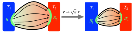
Figure 20: An arbitrarily shaped container in contact with two heat baths. The value of ${\tilde{T}}$ is unchanged with respect to the scale transformation of the container with fixing $T_{1}$ and $T_{2}$.

Hereafter, we show that $\alpha$ is a function of the geometry of the container and independent of ${\tilde{T}}$ and $p$. We consider a container as shown in Fig. 20, which is in contact with the first heat bath of $T_{1}$ in a region of the surface $\bm{B}_{1}$ and with the second bath of $T_{2}$ in $\bm{B}_{2}$. The rest of the surface of the container is thermally insulating. The steady profiles of temperature, density, and heat flux are $T(\bm{r})$, $\rho(\bm{r})$, and $\bm{j}(\bm{r})=-\kappa(T(\bm{r}),p)\nabla T$, respectively.

The profile $T(\bm{r})$ is determined by the condition $\nabla\cdot\bm{j}=0$ for the steady state, which is written as

$$\left\{\begin{array}[]{ll}&\nabla\cdot\left(\kappa({\tilde{T}},p)\nabla T(\bm{r})\right)=0,\\ &T(\bm{r}\in\bm{B}_{1})=T_{1},\quad T(\bm{r}\in\bm{B}_{2})=T_{2},\end{array}\right.$$ (10.41)

with an error of $O(\varepsilon^{2})$. By introducing a scale transformation $\bm{r}\rightarrow\bm{r}^{\prime}$

$$\bm{r}=\sqrt{\kappa({\tilde{T}},p)}~{}\bm{r}^{\prime},$$ (10.42)

as shown in Fig. 20, we express (10.41) as

$$\left\{\begin{array}[]{ll}&\Delta^{\prime}t(\bm{r}^{\prime})=0,\\ &t(\bm{r}^{\prime}\in\bm{B}_{1}^{\prime})=T_{1},\quad t(\bm{r}^{\prime}\in\bm{B}_{2}^{\prime})=T_{2},\end{array}\right.$$ (10.45)

where $t(\bm{r}^{\prime})=T\left(\sqrt{\kappa({\tilde{T}},p)}~{}\bm{r}^{\prime}\right)$. Letting the solution of (10.45) be $t_{*}(\bm{r}^{\prime})$, the global temperature is written as

$${\tilde{T}}=\frac{\int_{{\cal D}^{\prime}}d^{3}{\bm{r}^{\prime}}~{}\rho(t_{*}(\bm{r}^{\prime}),p)t_{*}(\bm{r}^{\prime})}{\int_{{\cal D}^{\prime}}d^{3}{\bm{r}^{\prime}}~{}\rho(t_{*}(\bm{r}^{\prime}),p)}.$$ (10.46)

We here expand $t_{*}(\bm{r}^{\prime})$ in $\Xi/T_{\mathrm{m}}$:

$$t_{*}(\bm{r}^{\prime})=T_{\mathrm{m}}\left(1+\frac{\Xi}{T_{\mathrm{m}}}\Phi(\bm{r}^{\prime})+O(\varepsilon^{2})\right),$$ (10.47)

$$T_{1}=T_{\mathrm{m}}-\frac{\Xi}{2},\quad T_{2}=T_{\mathrm{m}}+\frac{\Xi}{2}.$$ (10.48)

With these expansions, (10.45) is written as

$$\begin{array}[]{ll}&\Delta^{\prime}\Phi(\bm{r}^{\prime})=0,\\ &\Phi(\bm{r}^{\prime}\in\bm{B}_{1}^{\prime})=-\displaystyle\frac{1}{2},\quad\Phi(\bm{r}^{\prime}\in\bm{B}_{2}^{\prime})=\frac{1}{2}.\end{array}$$ (10.51)

It is obvious that the solution of (10.51) depends only on the geometry of the surface but is independent of the scale of the container and all physical parameters. More explicitly, we confirm that $\Phi(\bm{r}^{\prime})$ is independent of ${\tilde{T}}$ and $p$. (10.46) yields

$${\tilde{T}}-T_{\mathrm{m}} =\Xi\frac{\int_{{\cal D}^{\prime}}d^{3}{\bm{r}^{\prime}}~{}\rho(t_{*}(\bm{r}^{\prime}),p)\Phi(\bm{r}^{\prime})+O(\varepsilon)}{\int_{{\cal D}^{\prime}}d^{3}{\bm{r}^{\prime}}~{}\rho(t_{*}(\bm{r}^{\prime}),p)}$$

$$=\Xi\int_{{\cal D}^{\prime}}d^{3}{\bm{r}^{\prime}}~{}\Phi(\bm{r}^{\prime})+O(\varepsilon^{2}),$$ (10.52)

which indicates ${\tilde{T}}-T_{\mathrm{m}}$ is independent of ${\tilde{T}}$ and $p$.

At last, we examine the parameter $\alpha$ which is rewritten as

$$\alpha=\frac{1}{V^{\prime}}\int_{{\cal D}^{\prime}}d^{3}{\bm{r}^{\prime}}~{}\left(\frac{t_{*}(\bm{r}^{\prime})-{\tilde{T}}}{\Xi}\right)^{2}.$$ (10.53)

Using (10.47) and (10.52), we have

$$\alpha=\frac{1}{V^{\prime}}\int_{{\cal D}^{\prime}}d^{3}{\bm{r}^{\prime}}~{}\left[\Phi(\bm{r}^{\prime})-\int_{{\cal D}^{\prime}}d^{3}{\bm{r}^{\prime}}~{}\Phi(\bm{r}^{\prime})\right]^{2},$$ (10.54)

which is determined by the function $\Phi$ given by (10.51). For instance, calculating $\alpha$ for rectangular containers, we obtain

$$\alpha=\frac{1}{12}.$$ (10.55)

11 Concluding Remarks

In this long paper, we have developed a thermodynamic framework for heat conduction states, which we call global thermodynamics. The key concept of the framework is the global temperature defined by (2.54). We describe spatially inhomogeneous systems by a set of global thermodynamic variables. Although the method is rather different from a standard continuum description, global thermodynamics is built on local equilibrium thermodynamics and the transportation equation. Thus, it is not contradictory with established theories. Nevertheless, our framework provides a new prediction on the thermodynamic properties of a liquid-gas interface in heat conduction. As we explained in §4.4, the rule of connecting two phases at the interface is out of the standard hydrodynamics with local equilibrium thermodynamics. Even for this case, global thermodynamics can determine the way how to connect the two phases by the variational principle that is a natural extension of the Maxwell construction for equilibrium cases.

Although global thermodynamics is self-consistent, self-contained, and natural, it does not ensure the validity of the framework. Similarly to other universal theories such as thermodynamics, hydrodynamics, and statistical mechanics, global thermodynamics involves a fundamental assumption on the determination of the steady state. In other words, if our quantitative prediction on the phase coexistence is denied by experiments, global thermodynamics could not be valid. In this case, we will attempt to understand the experimental results carefully so that we have a correct description of phenomena out of equilibrium. This is of course quite stimulating, and we sincerely wait for experiments. Numerical simulations of microscopic dynamics such as molecular dynamics also provide useful materials for further studies. To the present, no deviation of the interface temperature from the transition temperature was observed Bedeaux00 ; Ogushi . We conjecture that this is due to the insufficiency of the separation of scales, because the deviation should be observed in systems with enough separation of scales, as discussed in Ref. SNIN .

Putting aside the ultimate validity of global thermodynamics, we emphasize that the framework itself is quite fruitful. This paper presents only the minimum backbone, but exhibits non-trivial simple relations among several quantities. These somewhat miraculous statements may suggest a deeper structure behind global thermodynamics. Moreover, importantly, the story does not end. We did not discuss the Clausius equality for the cases with a liquid-gas interface, while we confirmed it for single-phase systems in §3.3. The equality connects “heat” to the entropy change, and the “heat” should be defined as the renormalized one, called “excess heat”, after subtracting the persistent heat as we reviewed in Introduction. It is quite natural to study the liquid-gas coexistence by considering an extended form of the Clausius relation. Since we find that this provides another source of further development of the framework, we have decided to argue it in a separate paper.

From a theoretical viewpoint in a broad context, we expect that we may derive global thermodynamics based on a more microscopic description. Since we know the basic framework of non-equilibrium statistical mechanics, e.g. the linear response theory, we obtain a linear response formula of the temperature of the interface. It is quite formal, and it is not evident that the result satisfies the temperature relation (5.47). Related to this problem, recently, we have calculated the temperature of the interface for a stochastic order parameter equation describing the phase coexistence in heat conduction SNIN . The result shows that the interface temperature deviates from the equilibrium transition temperature. It should be noted that global thermodynamics can be formulated for systems that exhibits an order-disorder transition in heat conduction. By finding a connection between the two theories, we will understand a microscopic mechanism of the interesting macroscopic phenomenon.

Our theory may be naturally generalized to that for heat conduction systems where a liquid flows in and a gas flows out. When a steady state is observed, the system exhibits perpetual evaporation at the interface. The latent heat is persistently generated at the interface and as a result additional heat flux occurs from the interface to the liquid region and gas region. This phenomenon was experimentally studied for pure water Fang-Ward , and a macroscopic temperature gap as much as about $8$K was found at the liquid-gas interface. As a related phenomenon, the temperature gradient in the inverse direction to the imposed temperature difference was observed for the liquid-gas coexistence of a heat conducting Helium far from equilibrium Urban . These phenomena may be closely related to our prediction on the phase coexistence in heat conduction. We will attempt to explain such phenomena in global thermodynamics. Furthermore, we also expect that the description of global quantities may be useful for more complicated systems. Even for phenomena far from equilibrium such as motility-induced phase separation mips , there may be an appropriate set of global variables on the basis of local variables whose space-time evolution may be described by another evolution rule. We will accumulate such examples.

We hope that this paper is a good starting point of many studies.

References

- (1) Landau, L. D., Lifshitz, E. M. : Fluid Mechanics. Pergamon Press, Oxford (1959).
- (2) Zubarev, D. N. : Nonequilibrium Statistical Thermodynamics. Consultants Bureau, New York (1974).
- (3) Mclennan, J. A. : Phys. Fluids 3, 493-502 (1960); Introduction to Non-equilibrium Statistical Mechanics. Prentice-Hall (1988).
- (4) Onsager, L. : Reciprocal relations in irreversible processes. I. Phys. Rev. 37, 405-426 (1931); Reciprocal relations in irreversible processes. II. Phys. Rev. 38, 2265-2279 (1931).
- (5) de Groot, S. and Mazur, P. : Non-equilibrium Thermodynamics. North-Holland, Amsterdam (1962)
- (6) Schmitz, R. : Fluctuations in nonequilibrium fluids, Physics Reports 171, 1-58 (1988).
- (7) Kubo, R., Toda, M., Hashitsume, N. : Statistical Physics II. Springer, (1985).
- (8) Nakano, H. : Linear response theory - historical perspective. Int. J. Mod. Phys. B 7:2397-2467 (1993).
- (9) Zwanzig, R. : Memory Effects in Irreversible Thermodynamics, Phys. Rev. 124, 983-992 (1961).
- (10) Mori, H. : Transport, Collective Motion, and Brownian Motion, Prog. Theor. Phys. 33, 423-455 (1965)
- (11) Kawasaki, K., Gunton, J. D. : Theory of nonlinear transport processes: nonlinear shear viscosity and normal stress effects, Phys. Rev. A 8, 2048-2064 (1973).
- (12) Ashkin, A., Schütze, K., Dziedzic, J. M., Euteneuer, U., Schliwa, M. : Force generation of organelle transport measured in vivo by an infrared laser trap, Nature 348, 346-348 (1990).
- (13) Smith, S. B., Finzi, L. Bustamante, C. : Direct mechanical measurements of the elasticity of single DNA molecules by using magnetic beads, Science 258, 1122-1126 (1992).
- (14) Svoboda, K., Schmidt C. F., Schnapp B. J., Block, S. M. : Direct observation of kinesin stepping by optical trapping interferometry, Nature 365, 721-727 (1993).
- (15) Perkins, T. T., Quake, S. R., Smith, D. E., Chu, S. : Relaxation of a single DNA molecule observed by optical microscopy, Science 264, 822-826 (1994)
- (16) Noji, H., Yasuda, R., Yoshida, M., Kinosita Jr, K. : Direct observation of the rotation of F1-ATPase. Nature 386, 299-302 (1997).
- (17) Seifert, U. : Stochastic thermodynamics, fluctuation theorems and molecular machines, Rep. Prog. Phys. 75, 126001 (2012).
- (18) Sekimoto, K. : Stochastic Energetics, Lect. Notes Phys. 799. Springer-Verlag, Berlin (2010).
- (19) Klages, R., Just, W., Jarzynski, C. (eds.) : Nonequilibrium Statistical Physics of Small Systems. Wiley-VCH, Weinheim (2013)
- (20) Evans, D. J., Cohen, E. G. D., Morriss, G. P. : Probability of second law violations in shearing steady states, Phys. Rev. Lett. 71, 2401-2404 (1993).
- (21) Jarzynski, C. : Nonequilibrium equality for free energy differences, Phys. Rev. Lett. 78, 2690-2693 (1997).
- (22) Gallavotti, G., Cohen, E. G. D. : Dynamical Ensembles in Nonequilibrium Statistical Mechanics, Phys. Rev. Lett. 74, 2694-2697 (1995).
- (23) Kurchan, J. : Fluctuation theorem for stochastic dynamics, J. Phys. A: Math. Gen. 31, 3719-3729 (1998).
- (24) Lebowitz, J. L., Spohn, H. : A Gallavotti–Cohen-type symmetry in the large deviation functional for stochastic dynamics, J. Stat. Phys. 95, 333-365 (1999).
- (25) Maes, C. : The fluctuation theorem as a Gibbs property, J. Stat. Phys. 95, 367-392 (1999).
- (26) Crooks, G. E. : Entropy production fluctuation theorem and the nonequilibrium work relation for free energy differences, Phys. Rev. E 60, 2721-2726 (1999).
- (27) Jarzynski, C. : J. Stat. Phys. 98, 77-102 (2000)
- (28) Crooks, G. : Path ensembles averages in systems driven far-from-equilibrium, Phys. Rev. E 61, 2361-2366 (1999).
- (29) Komatsu, T. S., Nakagawa, N. : Expression for the stationary distribution in nonequilibrium steady states, Phys. Rev. Lett. 100, 030601 (2008).
- (30) Komatsu, T. S., Nakagawa, N., Sasa, S.-i., Tasaki, H. : Representation of nonequilibrium steady states in large mechanical systems, J. Stat. Phys. 134, 401-423 (2009).
- (31) Maes, C., Netočný, K. : Rigorous meaning of McLennan ensembles, J. Math. Phys. 51, 015219 (2010).
- (32) Sasa, S.-i. : Derivation of Hydrodynamics from the Hamiltonian Description of Particle Systems, Phys. Rev. Lett. 112, 100602 (2014).
- (33) Bodineau, T., Derrida, D. : Current fluctuations in nonequilibrium diffusive systems: an additivity principle, Phys. Rev. Lett. 92, 180601 (2004).
- (34) Bertini, L., De Sole, A., Gabrielli, D., Jona-Lasinio, G., Landim, C. : Current fluctuations in stochastic lattice gases’, Phys. Rev. Lett. 94, 030601 (2005).
- (35) Maes, C., Netočný, K. : Minimum entropy production principle from a dynamical fluctuation law, J. Math. Phys. 48, 053306 (2007).
- (36) Nemoto, T., Sasa, S.-i. : Thermodynamic formula for the cumulant generating function of time-averaged current, Phys. Rev. E 84, 061113 (2011).
- (37) Bertini, L., De Sole, A., Gabrielli, D., Jona-Lasinio, G., Landim, C. : Macroscopic fluctuation theory, Rev. Mod. Phys. 87, 593-636 (2015).
- (38) Parrondo, J. M. R., Horowitz, J. M., Sagawa, T. : Thermodynamics of information, Nature Physics 11, 131-139 (2015).
- (39) Sasa, S.-i., Nakagawa, N., Itami, M., Nakayama, N. : Stochastic order parameter dynamics for phase coexistence in heat conduction, in preparation.
- (40) Jaynes, E. T. : The minimum entropy production principle, Ann. Rev. Phys. Chem. 31, 579- 601 (1980).
- (41) Klein, M. J., Meijer, P. H. E. : Principle of minimum entropy production, Phys. Rev. 96, 250-255 (1954).
- (42) Callen, H. B., Thermodynamics and an Introduction to Thermostatistics, 2nd ed. Wiley, New York (1985)
- (43) Prigogine, I., Kondepudi, D. : Modern Thermodynamics : From Heat Engines to Dissipative Structures, Second Edition. Wiley, Chichester (1998)
- (44) Einstein, A. : Theorie der Opaleszenz von homogenen Flüsigkeiten und Flüssigkeitsgemischen in der Nähe des kritischen Zustandes, (The Theory of the Opalescence of Homogeneous Fluids and Liquid Mixtures near the Critical State), Annalen der Physik 33, 1275 - 1298, (1910).
- (45) Oono, Y. : Perspectives on Statistical Thermodynamics. Cambridge University Press (2017)
- (46) Keizer, J. : Statistical thermodynamics of nonequilibrium processes. Springer, (1987)
- (47) Eu, B. C. : Kinetic Theory and Irreversible Thermodynamics. Wiley, New York (1992)
- (48) Jou, D., Casas-Vazquez, J., Lebon, G. : Extended Irreversible Thermodynamics 3rd revised and enlarged edn. Springer, Berlin (2001)
- (49) Bedeaux, D. : Nonequilibrium thermodynamics and statistical physics of surfaces, Adv. Chem. Phys. 64 47-109 (1986).
- (50) Casas-Vazquez, J., Jou, D. : Temperature in non-equilibrium states: a review of open problems and current proposals, Rep. Prog. Phys. 66, 1937-2023 (2003).
- (51) Sasa, S.-i., Tasaki, H. : Steady state thermodynamics, J. Stat. Phys. 125, 125-224 (2006).
- (52) Hayashi, K., Sasa, S.-i. : Thermodynamic relations in a driven lattice gas: numerical experiments. Phy. Rev. E 68, 035104(R) (2003).
- (53) Bertin, E., Martens, K., Dauchot, O., Droz, M. : Intensive thermodynamic parameters in nonequilibrium systems, Phys. Rev. E 75, 031120 (2007).
- (54) Pradhan, P., Ramsperger, R., Seifert, U. : Approximate thermodynamic structure for driven lattice gases in contact, Phys. Rev. E 84, 041104 (2011).
- (55) Dickman, R. : Failure of steady-state thermodynamics in nonuniform driven lattice gases, Phys. Rev. E 90, 062123 (2014).
- (56) Landauer, R. : far from equilibrium, Phys. Rev. A 18, 255-266 (1978)
- (57) Oono, Y., Paniconi, M. : Steady state thermodynamics, Prog. Theor. Phys. Suppl. 130, 29-44 (1998).
- (58) Hatano, T., Sasa, S.-i. : Steady-state thermodynamics of Langevin systems, Phys. Rev. Lett. 86, 3463-3466 (2001).
- (59) Ruelle, D. : Proc. Natl. Acad. Sci. U.S.A. 100, 3054 (2003).
- (60) Komatsu, T. S., Nakagawa, N., Sasa, S.-i., Tasaki, H. : Steady-state thermodynamics for heat conduction: Microscopic derivation, Phys. Rev. Lett. 100, 230602 (2008).
- (61) Nakagawa, N. : Work relation and the second law of thermodynamics in nonequilibrium steady states, Phys. Rev. E 85, 051115 (2012).
- (62) Bertini, L., De Sole, A., Gabrielli, D., Jona-Lasinio, G., Landim, C. : Clausius inequality and optimality of quasistatic transformations for nonequilibrium stationary states, Phys. Rev. Lett. 110, 020601 (2013).
- (63) Maes, C., Netočný, K. : A nonequilibrium extension of the Clausius heat theorem, J. Stat. Phys. 154, 188-203 (2014).
- (64) Spinney, R. E., Ford, I. J. : Nonequilibrium Thermodynamics of Stochastic Systems with Odd and Even Variables, Phys. Rev. Lett. 108, 170603 (2012).
- (65) Chiba, Y., Nakagawa, N. : Numerical determination of entropy associated with excess heat in steady-state thermodynamics, Phys. Rev. E 94, 022115 (2016).
- (66) Nakagawa, N., Sasa, S.-i. : Liquid-Gas Transitions in Steady Heat Conduction, Phys. Rev. Lett. 119, 260602 (2017)
- (67) Røsjorde, A., Fossmo, W. D., Bedeaux, D., Kjelstrup, S., Hafskjold, B. : Nonequilibrium molecular dynamics simulations of steady-state heat and mass transport in condensation: I. Local equilibrium, J. Coll. Int. Sci. 232, 178-185 (2000).
- (68) Ogushi, F., Yukawa, S., Ito, N. : Asymmetric structure of gas-liquid interface, J. Phys. Soc. Jpn. 75, 073001 (2006).
- (69) Bedeaux, D., Johannessen, E., Røsjorde, A. : The nonequilibrium van der Waals square gradient model.(I). The model and its numerical solution, Physica A 330, 329-353 (2003).
- (70) Onuki, A., Dynamic van der Waals theory, Phys. Rev. E 75, 036304 (2007).
- (71) Iso, N., Uematsu, K., Mashimo, K. : Kiso Butsuri Kagaku. Tokyo Kyogakusha, Tokyo (1997)
- (72) NIST Chemistry WebBook, SRD69. https://webbook.nist.gov/chemistry/
- (73) Kim, H. D., Hayakawa, H. : Kinetic theory of a dilute gas system under steady heat conduction. J. Phys. Soc. Jpn. 72, 1904-1916 (2003); 73, 1609 (2003).
- (74) Aoki, K. Kusnezov, D. : On the violations of local equilibrium and linear response, arXiv:nlin/0105063.
- (75) Wada, H., Sasa, S.-i. : Anomalous pressure in fluctuating shear flow, Phys. Rev. E 67, 065302(R) (2003).
- (76) Kirkpatrick, T. R., Ortiz de Zárate, J. M., Sengers, J. V. : Fluctuation-induced pressures in fluids in thermal nonequilibrium steady states, Phys. Rev. E 89, 022145 (2014).
- (77) Fang, G., Ward, C. A. : Temperature measured close to the interface of an evaporating liquid, Phys. Rev. E 59, 417-428 (1999)
- (78) Urbana, P., Schmoranzerb, D., Hanzelkaa, P., Sreenivasanc, K. R., Skrbekb, L. : Anomalous heat transport and condensation in convection of cryogenic helium, Proc. Nat. Acad. Sci. 110, 8036-8039 (2013).
- (79) Cates, M. E., Tailleur, J. : Motility-Induced Phase Separation, Annual Review of Condensed Matter Physics 6, 219-244 (2015).