First-order primal-dual algorithm with Correction

Abstract

This paper is devoted to the design of efficient primal-dual algorithm (PDA) for solving convex optimization problems with known saddle-point structure. We present a new PDA with larger acceptable range of parameters and correction, which result in larger step sizes. The step sizes are predicted by using a local information of the linear operator and corrected by linesearch to satisfy a very weak condition, even weaker than the boundedness of sequence generated. The convergence and ergodic convergence rate are established for general cases, and in case when one of the prox-functions is strongly convex. The numerical experiments illustrate the improvements in efficiency from the larger step sizes and acceptable range of parameters.

1 Introduction

Let $X$, $Y$ be two finite-dimensional real vector spaces equipped with an inner product $\langle\cdot,\cdot\rangle$ and its corresponding norm $\|\cdot\|=\sqrt{\langle\cdot,\cdot\rangle}$. We focus on the following primal problem

$$\min_{x\in X}f(Kx)+g(x),$$ (1)

where

• $K:X\rightarrow Y$ is a bounded linear operator, with operator norm $L=\|K\|$;

• $f:\rightarrow(-\infty,+\infty]$ and $g:X\rightarrow(-\infty,+\infty]$ are proper lower semicontinuous convex functions.

Let $f^{*}$ denotes the Legendre-Fenchel conjugate of the function $f$, and $K^{*}$ the adjoint of the operator $K$, then $f^{*}$ is a proper, convex, lower-semicontinuous (l.s.c.) function. The dual problem of (1) reads as:

$$\min_{y\in Y}f^{*}(y)+g^{*}(-K^{*}y).$$ (2)

Actually, problem (1) together with its dual (2) is equivalent to the following convex-concave saddle point problem

$$\min_{x\in X}\max_{y\in Y}~{}~{}g(x)+\langle Kx,y\rangle-f^{*}(y).$$ (3)

By introducing an auxiliary variable $z$, problem (1) can be written as two-block separable convex optimization:

$$\min\;\; f(z)+g(x)$$

$$s.t.\;\; Kx-z=0,$$

$$x\in X,~{}~{}z\in Y.$$

The convex-concave saddle point problem (3) and its primal problem with forms (1) and (1) are widely presented in many disciplines, including mechanics, signal and image processing, and economics app1 ; app2 ; app3 ; app4 ; statistical_learning ; 11. ; FB-Tseng . Saddle point problems are ubiquitous in optimization as it is a very convenient way to represent many nonsmooth problems, and it in turn often allows to improve the complexity rates from ${\mathcal{O}}(1/\sqrt{N})$ to ${\mathcal{O}}(1/N)$. However, the saddle point problem (3) is a typical example where the two simplest iterative methods, the forward-backward method and the Arrow-Hurwicz method AH , will not work.

Many efficient methods have been proposed for solving problem (3), for instance, alternating direction method of multipliers (ADMM) statistical_learning ; PC-ADMM ; He_ADMM-based ; ADMM , extrapolational gradient methods 6. ; extragradient ; extragradient-type ; 13. , primal-dual algorithms (PDA) PC-PDA ; CP_PDA ; He_PDA ; zhang_PDA ; inertial-FBF and their accelerated and generalized versions Nesterov2004 ; Acc_PDA ; M_PDA . Here, we concentrate on the most simple first-order PDA and its acceleration. The iterative scheme of the original PDA CP_PDA ; PC-PDA ; M_PDA with fixed step sizes reads as

$$\left.\begin{array}[]{l}y_{n+1}={\rm Prox}_{\sigma f^{*}}(y_{n}+\sigma Kz_{n}),\\ x_{n+1}={\rm Prox}_{\tau g}(x_{n}-\tau K^{*}y_{n+1}),\\ z_{n+1}=x_{n+1}+\delta(x_{n+1}-x_{n}),\end{array}\right\}$$ (8)

where $\delta$ is called an extrapolation parameter, $\tau>0$ and $\sigma>0$ are regarded as step sizes. When $\delta=0$ in (8), the primal-dual procedure (8) reduces to the Arrow-Hurwicz algorithm AH-PDA , which has been highlighted in zhu_TV for TV image restoration problems. In CP_PDA , it was shown that the primal-dual procedure (8) is closely related to many existing methods including the extrapolational gradient method Popov , the Douglas-Rachford splitting method DR-splitting , and the ADMM.

The convergence of (8) was proved in CP_PDA under assumptions $\delta=1$ and $\tau\sigma L^{2}<1$. Of course, it requires knowing the operator norm $L$ of $K$ to determine step sizes, namely, one need to compute the maximal eigenvalue $\lambda_{\max}(K^{*}K)$. For simple and sparse $K$ it can not matter, however, for large scale dense matrix $K$ computation of norm is much more expensive. Moreover, the eigenvalues of $K^{*}K$ can be quite different, so the step sizes governed by the maximal eigenvalue will be very conservative. As first-order algorithm, PDA suffers from slow convergence especially on poorly conditioned problems, when they may take thousands of iterations and still struggle reaching just four digits of accuracy Acc_PDA . As a remedy for the slow convergence, diagonal PC-PDA and non-diagonal precondition Acc_PDA were proposed, numerical efficiency can be improved for some cases, but still there is no strong evidence that such precondition improves or at least does not worsen the speed of convergence of PDA.

Generally, larger step sizes often yield a faster convergence, a linesearch thus was introduced to gain the speed improvement in M_PDA . It is known that, the linesearch requires the extra proximal operator or evaluations of $K$, or even both in every linesearch iteration, they will turn to be computationally expensive in situations, where the condition to satisfy is strong and the proximal operator is hard to compute and somewhat expensive. The linesearch in M_PDA is to find a proper step size $\tau_{n}$ satisfying

$$\sqrt{\beta}\tau_{n}\|K^{*}y_{n+1}-K^{*}y_{n}\|\leq\alpha\|y_{n+1}-y_{n}\|$$ (9)

with $\beta>0$ and $\alpha\in(0,1)$. The important parameter $\alpha$ relating to the step size was restricted on $\alpha\in]0,1[$ for guaranteeing the convergence, which will hamper larger step sizes.

Contributions. Our purpose here is to propose an efficient PDA with a prediction-correction procedure (PDA-C for short) to estimate step sizes, rather than using the norm of $K$. The main contribution can be summarized as follows:

• We extend the range of $\delta$ to $]\frac{\sqrt{5}-1}{2},+\infty[$, obtain a larger value of $\alpha<\frac{1}{\sqrt{\delta}}$. Namely, $\delta$ can be less than 1 and $\alpha$ can close to $\sqrt{\phi}\approx 1.272$ ($\phi=\frac{\sqrt{5}+1}{2}$ is the golden ratio), which will extend the range of step sizes.

• The step sizes are predicted with low computational cost, by the aid of an inverse local Lipschitz constant of $K^{*}$, and then corrected when $\delta<1$ to satisfy a very weak condition $\|x_{n+1}-x_{n}\|<+\infty$. For all the tested problems shown in Section 5, this condition is so weak that the linesearch in Correction step does not start or run only a few times to arrive termination conditions.

• We prove that PDA-C converges with ergodic rate ${\mathcal{O}}(1/N)$ for the primal-dual gap, and introduce an accelerated version of PDA-C under the assumption that the primal or dual problem is strongly convex. The theoretical rate of convergence can be further improved to yield an ergodic rate of convergence ${\mathcal{O}}(1/N^{2})$ for the primal-dual gap.

The paper is organized as follows. In Section 2, we provide some useful facts and notations. Section 3 is devoted to our basic PDA with correction and updating step sizes. We prove the convergence and establish the ergodic convergence rate for the primal-dual gap. In Section 4 we propose an accelerated version of PDA-C under the assumption that the primal or dual problem is strongly convex. The implementation and numerical experiments, for solving the LASSO, min-max matrix game and nonnegative least square, are provided in Section 5. We conclude our paper in the final section.

2 Preliminaries

We state the following notations and facts on the well-known properties of the proximal operator and Young’s inequality. Some properties are included in textbooks such as Bauschke2011Convex .

Let $g:X\rightarrow(-\infty,+\infty]$ be a proper lower semicontinuous convex functions, the proximal operator ${\rm Prox}_{\lambda g}:X\rightarrow X$ is defined as ${\rm Prox}_{\lambda g}(x)=(I+\lambda\partial g)^{-1}(x),\lambda>0,x\in X$, and explicitly as

$${\rm Prox}_{\lambda g}(x)=\operatorname*{argmin}_{y\in X}\left\{g(y)+\frac{1}{2\lambda}\|x-y\|^{2}\right\},\quad\forall\,x\in X,\lambda>0.$$

Fact 1

Bauschke2011Convex Let $g:X\rightarrow(-\infty,+\infty]$ be a convex function. Then for any $\lambda>0$ and $x\in X$, $p={\rm Prox}_{\lambda g}(x)$ if and only if

$$\langle p-x,y-p\rangle\geq\lambda[g(p)-g(y)],~{}~{}\forall y\in X.$$

Fact 2

Let $\{a_{n}\}_{n\in{\mathbb{N}}}$, $\{b_{n}\}_{n\in{\mathbb{N}}}$ be two nonnegative real sequences and $\exists N>0$ such that

$$a_{n+1}\leq a_{n}-b_{n},~{}~{}\forall n>N.$$

Then $\{a_{n}\}_{n\in{\mathbb{N}}}$ is convergent and $\lim_{n\rightarrow\infty}b_{n}=0$.

Fact 3

(Young’s inequality) For any $a,b\geq 0$ and $\varepsilon>0$, we have

$$ab\leq\frac{a^{2}}{2\varepsilon}+\frac{\varepsilon b^{2}}{2}.$$

The following identity (cosine rule) appears in many convergence analyses and we will use it many times. For any $x,y,z\in{\mathbb{R}}^{n}$,

$$\langle x-y,x-z\rangle=\frac{1}{2}\|x-y\|^{2}+\frac{1}{2}\|x-z\|^{2}-\frac{1}{2}\|y-z\|^{2}.$$ (10)

We assume that the solution set of problem (3) is nonempty and denoted by ${\mathcal{S}}$. Let $(\bar{x},\bar{y})$ be a saddle point of problem (3), i.e. $(\bar{x},\bar{y})\in{\mathcal{S}}$, it therefore satisfies

$$K\bar{x}\in\partial f^{*}(\bar{y}),~{}~{}-(K^{*}\bar{y})\in\partial g(\bar{x}),$$

where $\partial f^{*}$ and $\partial g$ are the subdifferential of the convex functions $f^{*}$ and $g$. For more details on the theory of saddle point, see Bauschke2011Convex . Throughout the paper we will assume that $f$ and $g$ are proper (or simple), in the sense that their resolvent operator has a closed-form representation.

By the definition of saddle point, for any $(\bar{x},\bar{y})\in{\mathcal{S}}$ we have

$$P_{\bar{x},\bar{y}}(x):=g(x)-g(\bar{x})+\langle K^{*}\bar{y},x-\bar{x}\rangle\geq 0,~{}\forall x\in X,$$ (11)

$$D_{\bar{x},\bar{y}}(y):=f^{*}(y)-f^{*}(\bar{y})-\langle K\bar{x},y-\bar{y}\rangle\geq 0,~{}\forall y\in Y.$$ (12)

The primal-dual gap can be expressed as $G_{\bar{x},\bar{y}}(x,y)=P_{\bar{x},\bar{y}}(x)+D_{\bar{x},\bar{y}}(y)$. In certain cases when it is clear which saddle point is considered, we will omit the subscript in $P$, $D$ and $G$. It is also important to highlight that functions $P(\cdot)$ and $D(\cdot)$ are convex for fixed $(\bar{x},\bar{y})\in{\mathcal{S}}$.

3 Primal-Dual Algorithm with Correction

In this section, we state our primal-dual algorithm with correction and explore its convergence. The step sizes are predicted by the aid of an inverse local Lipschitz constant of $K^{*}$ and corrected using linesearch.

 

Algorithm 1 (PDA-C for solving (3))

Step 0.

Take $\delta\in]\frac{\sqrt{5}-1}{2},+\infty[$, $\varrho\in]0,1[$ and $1<\nu\leq\mu$. Choose $x_{0}\in X,$ $y_{0}\in Y$, $\lambda_{0}=\lambda_{1}>0$, $\beta>0$ and $\alpha\in]0,\frac{1}{\sqrt{\delta}}[$. Set $n=0$ and

$$\zeta_{0}=\max\{\|x_{0}-{\rm Prox}_{\lambda_{0}g}(x_{0}-\lambda_{0}K^{*}y_{0})\|,~{}~{}\|y_{0}-{\rm Prox}_{\lambda_{0}f^{*}}(y_{0}+\beta\lambda_{0}Kx_{0})\|\}.$$

Step 1.

1.a. Compute

$$x_{n+1} = {\rm Prox}_{\lambda_{n}g}(x_{n}-\lambda_{n}K^{*}y_{n}),$$ (13)

1.b. Correct when $\delta<1$: compute $\zeta_{n+1}=\|x_{n+1}-x_{n}\|$, check

$$\zeta_{n+1}\leq\min\{\mu\zeta_{0},~{}~{}\nu\zeta_{n}\},$$ (14)

if not hold, set $\lambda_{n}\leftarrow\varrho\lambda_{n}$, $\lambda_{n+1}\leftarrow\min\{\lambda_{n},\lambda_{n+1}\}$ and return to Step 1.a.

Step 2.

Compute

$$z_{n+1} = x_{n+1}+\delta(x_{n+1}-x_{n}),$$

$$y_{n+1} = {\rm Prox}_{\lambda_{n+1}f^{*}}(y_{n}+\beta\lambda_{n+1}Kz_{n+1}),$$ (15)

and update

$$\lambda_{n+2} = \left\{\begin{array}[]{cl}\min~{}\left\{{\frac{\alpha\|y_{n+1}-y_{n}\|}{\sqrt{\beta}\|K^{*}y_{n+1}-K^{*}y_{n}\|},~{}~{}\lambda_{n+1}}\right\},&\mbox{if}\ \ K^{*}y_{n+1}-K^{*}y_{n}\neq 0,\\ \lambda_{n+1},&\mbox{otherwise};\end{array}\right.$$ (18)

Step 3.

Set $n\leftarrow n+1$ and return to step 1.

 

Remark 1

For brevity of establishing convergence, different step sizes $\lambda_{n}$ and $\lambda_{n+1}$ are used in (13) and (15), respectively. So we have to take two step sizes to compute $x_{n+1}$ and $y_{n+1}$, then obtain the next step size $\lambda_{n+2}$ during each iteration. Furthermore, if $\delta=1$, then $\alpha<1$, in this sense the step sizes agree with that introduced in CP_PDA ; M_PDA .

Remark 2

Note that the primal and dual variables are symmetrical in the problem (3) and PDA-C, we thus choose a variable with simple proximal operator to correct. In practice, there are many functions with linear (or affine) proximal operator, for instance, $\langle a,x\rangle$, $\frac{1}{2}\|x-a\|^{2}$ and the indicator function $l_{C}(x)$ with $C=\{y:\langle a,y\rangle=b\}$ or $C={\mathbb{B}}(c,r)$, a closed ball with a center $c$ and a radius $r>0$. For these functions, the linesearch becomes extremely simple: it does not require any additional matrix-vector multiplications.

The aim of Correction step is to bound $\{\|x_{n+1}-x_{n}\|\}$ when $\delta<1$, as convergence analysis requires $\|x_{n+1}-x_{n}\|<+\infty$. From (14), we have $\zeta_{n}\leq\nu\zeta_{0}$ for all $n\geq 1$, and $\zeta_{n+1}\leq\mu\zeta_{n}$ for bounding more tightly due to $\|x_{n+1}-x_{n}\|\rightarrow 0$. The following lemma shows that the correction procedure described in Algorithm 1 is well-defined.

Lemma 1

The correction procedure always terminates. i.e., $\{\lambda_{n}\}$ is well defined when $\delta\in]\frac{\sqrt{5}-1}{2},1[$.

Proof. Denote

$$A:=\partial g~{}~{}\mbox{and}~{}~{}x_{n+1}(\lambda):=\mbox{prox}_{\lambda g}(x_{n}-\lambda K^{*}y_{n}).$$

From (Bauschke2011Convex, , Theorem 23.47), we have that $\mbox{prox}_{\lambda g}[x_{n+1}(0)]\rightarrow P_{\overline{\operatorname*{dom}A}}[x_{n+1}(0)]$ as $\lambda\rightarrow 0$ ($\overline{\operatorname*{dom}A}$ denotes the closures of $\operatorname*{dom}A$), which together with the nonexpansivity of $\mbox{prox}_{\lambda g}$ yields

$$\|x_{n+1}(\lambda)-P_{\overline{\operatorname*{dom}A}}[x_{n+1}(0)]\|$$

$$\leq \|x_{n+1}(\lambda)-\mbox{prox}_{\lambda g}[x_{n+1}(0)]\|+\|\mbox{prox}_{\lambda g}[x_{n+1}(0)]-P_{\overline{\operatorname*{dom}A}}[x_{n+1}(0)]\|$$

$$\leq \lambda\|F(y_{n})\|+\|\mbox{prox}_{\lambda g}[x_{n+1}(0)]-P_{\overline{\operatorname*{dom}A}}[x_{n+1}(0)]\|.$$

By taking the limit as $\lambda\rightarrow 0$, we deduce that $x_{n+1}(\lambda)\rightarrow P_{\overline{\operatorname*{dom}A}}[x_{n+1}(0)]$. Notice that $x_{n+1}(0)=x_{n}$, we observe $P_{\overline{\operatorname*{dom}A}}[x_{n+1}(0)]=x_{n}$.

By a contradiction, suppose that the correction procedure in Algorithm 1 fails to terminate at the $n$-th iteration. Then, for all $\lambda=\varrho^{i}\lambda_{n}$ with $i=0,1,\cdots$, we have $\|x_{n+1}(\lambda)-x_{n}\|>\min\{\mu\zeta_{0},\nu\zeta_{n}\}$. Since $\varrho^{i}\rightarrow 0$ as $i\rightarrow\infty$, so $\lambda\rightarrow 0$, this gives a contradiction $0\geq\min\{\mu\zeta_{0},\nu\zeta_{n}\}$, which completes the proof. $\Box$

Lemma 2

Let $\{\lambda_{n}\}_{n\in{\mathbb{N}}}$ be a sequence generated by PDA-C, then $\{\lambda_{n}\}_{n\in{\mathbb{N}}}$ is bounded, $\lim\limits_{n\rightarrow\infty}\lambda_{n}>0$ and $\lim\limits_{n\rightarrow\infty}\frac{\lambda_{n}}{\lambda_{n-1}}=1$.

Proof. First, $\{\lambda_{n}\}_{n\in{\mathbb{N}}}$ is upper bounded. Note that $K^{*}$ is a $L$-Lipschitz continuous mapping with $L=\|K\|$, we have

$$\frac{\alpha\|y_{n+1}-y_{n}\|}{\|K^{*}y_{n+1}-K^{*}y_{n}\|}\geq\frac{\alpha\|y_{n+1}-y_{n}\|}{L\|y_{n+1}-y_{n}\|}=\frac{\alpha}{L}$$

for $K^{*}y_{n+1}-K^{*}y_{n}\neq 0$. This implies the predicted step $\{\lambda_{n}\}_{n\in{\mathbb{N}}}$ has a lower bound $\tau=\min\{\frac{\alpha}{\sqrt{\beta}L},\lambda_{0}\}$, then $\lambda_{n}\geq\tau$ when $\delta\geq 1$. If $\delta<1$, $\{\lambda_{n}\}$ is well defined from Lemma 1, and has a lower bound $\tau=\min\{{\frac{\varrho^{i_{0}}\alpha}{\sqrt{\beta}L},\lambda_{0}}\}$ for some $i_{0}\geq 0$. Notice that the sequence $\{\lambda_{n}\}$ is monotonically decreasing, we have $\lambda=\lim\limits_{n\rightarrow\infty}\lambda_{n}>0$, consequently, $\lim\limits_{n\rightarrow\infty}\frac{\lambda_{n}}{\lambda_{n-1}}=1$. $\Box$

The properties of the generated step sizes, shown in Lemma 2, are vital for establishing convergence of PDA-C. In sequel, we give an observation in detail on the convergence by using this properties.

3.1 Convergence Analysis

This section devotes to the convergence theorem of PDA-C. First, we give the following lemmas for any $\delta\in]\frac{\sqrt{5}-1}{2},+\infty[$, which play a crucial role in the proof of the main theorem.

Lemma 3

Let $(\bar{x},\bar{y})\in{\mathcal{S}}$, and $\{(x_{n},y_{n})\}_{n\in{\mathbb{N}}}$ be a sequence generated by PDA-C. Define

$$\eta_{n}:=(1+\delta)P(x_{n})-\delta P(x_{n-1})+D(y_{n}),$$ (19)

then for any $(x,y)\in X\times Y$, we have

$$\lambda_{n}\eta_{n} \leq \langle x_{n+1}-x_{n},\bar{x}-x_{n+1}\rangle+\left\langle\frac{1}{\beta}(y_{n}-y_{n-1}),\bar{y}-y_{n}\right\rangle+\left\langle\frac{\lambda_{n}(z_{n}-x_{n})}{\delta\lambda_{n-1}},x_{n+1}-z_{n}\right\rangle$$

$$+\lambda_{n}\langle K^{*}y_{n}-K^{*}y_{n-1},z_{n}-x_{n+1}\rangle.$$

Proof. By (13), (15) and Fact 1, we have

$$\langle x_{n+1}-x_{n}+\lambda_{n}K^{*}y_{n},~{}~{}\bar{x}-x_{n+1}\rangle\geq\lambda_{n}[g(x_{n+1})-g(\bar{x})],$$ (20)

$$\left\langle\frac{1}{\beta}(y_{n}-y_{n-1})-\lambda_{n}Kz_{n},~{}~{}\bar{y}-y_{n}\right\rangle\geq\lambda_{n}[f^{*}(y_{n})-f^{*}(\bar{y})].$$ (21)

Similarly as in (20), for any $x\in X$ we have

$$\langle x_{n}-x_{n-1}+\lambda_{n-1}K^{*}y_{n-1},~{}~{}x-x_{n}\rangle\geq\lambda_{n-1}[g(x_{n})-g(x)].$$

Substituting $x=x_{n+1}$ and $x=x_{n-1}$ in the inequality above, we obtain

$$\langle x_{n}-x_{n-1}+\lambda_{n-1}K^{*}y_{n-1},~{}~{}x_{n+1}-x_{n}\rangle\geq\lambda_{n-1}[g(x_{n})-g(x_{n+1})],$$ (22)

$$\langle x_{n}-x_{n-1}+\lambda_{n-1}K^{*}y_{n-1},~{}~{}x_{n-1}-x_{n}\rangle\geq\lambda_{n-1}[g(x_{n})-g(x_{n-1})].$$ (23)

Multiplying (23) by $\delta$ and then adding it to (22) yields

$$\langle x_{n}-x_{n-1}+\lambda_{n-1}K^{*}y_{n-1},~{}~{}x_{n+1}-z_{n}\rangle\geq\lambda_{n-1}[(1+\delta)g(x_{n})-g(x_{n+1})-\delta g(x_{n-1})],$$ (24)

where we use $z_{n}=x_{n}+\delta(x_{n}-x_{n-1})$. Multiplying (24) by $\frac{\lambda_{n}}{\lambda_{n-1}}$ and using $z_{n}=x_{n}+\delta(x_{n}-x_{n-1})$ again, we get

$$\left\langle\frac{\lambda_{n}(z_{n}-x_{n})}{\delta\lambda_{n-1}}+\lambda_{n}K^{*}y_{n-1},~{}~{}x_{n+1}-z_{n}\right\rangle\geq\lambda_{n}[(1+\delta)g(x_{n})-g(x_{n+1})-\delta g(x_{n-1})].$$ (25)

Note that

$$\langle K^{*}y_{n}-K^{*}\bar{y},~{}~{}z_{n}-\bar{x}\rangle=\langle Kz_{n}-K\bar{x},~{}~{}y_{n}-\bar{y}\rangle,$$ (26)

adding (20) and (21) to (25) gives

$$\langle x_{n+1}-x_{n},\bar{x}-x_{n+1}\rangle+\left\langle\frac{1}{\beta}(y_{n}-y_{n-1}),\bar{y}-y_{n}\right\rangle+\left\langle\frac{\lambda_{n}(z_{n}-x_{n})}{\delta\lambda_{n-1}},x_{n+1}-z_{n}\right\rangle$$ (27)

$$+\lambda_{n}\langle K^{*}y_{n}-K^{*}y_{n-1},~{}~{}z_{n}-x_{n+1}\rangle-\lambda_{n}\langle K^{*}\bar{y},~{}~{}z_{n}-\bar{x}\rangle+\lambda_{n}\langle K\bar{x},~{}~{}y_{n}-\bar{y}\rangle$$

$$\geq \lambda_{n}[f^{*}(y_{n})-f^{*}(\bar{y})]+\lambda_{n}[(1+\delta)g(x_{n})-g(\bar{x})-\delta g(x_{n-1})].$$

Recalling the definitions of $P$ and $D$ in (11) and (12), and

$$(1+\delta)g(x_{n})-g(\bar{x})-\delta g(x_{n-1})+\langle K^{*}\bar{y},z_{n}-\bar{x}\rangle$$

$$= (1+\delta)[g(x_{n})-g(\bar{x})+\langle K^{*}\bar{y},x_{n}-\bar{x}\rangle]-\delta[g(x_{n-1})-g(\bar{x})+\langle K^{*}\bar{y},x_{n-1}-\bar{x}\rangle]$$

$$= (1+\delta)P(x_{n})-\delta P(x_{n-1}),$$

we can rewrite (27) as

$$\langle x_{n+1}-x_{n},\bar{x}-x_{n+1}\rangle+\left\langle\frac{1}{\beta}(y_{n}-y_{n-1}),\bar{y}-y_{n}\right\rangle+\left\langle\frac{\lambda_{n}(z_{n}-x_{n})}{\delta\lambda_{n-1}},x_{n+1}-z_{n}\right\rangle$$

$$+\lambda_{n}\langle K^{*}y_{n}-K^{*}y_{n-1},z_{n}-x_{n+1}\rangle$$

$$\geq \lambda_{n}[D(y_{n})+(1+\delta)P(x_{n})-\delta P(x_{n-1})].$$

The proof can be completed with the definition of $\eta_{n}$ in (19). $\Box$

Lemma 4

Let $(\bar{x},\bar{y})\in{\mathcal{S}}$, and $\{(x_{n},y_{n})\}_{n\in{\mathbb{N}}}$ be a sequence generated by PDA-C. Then, for any $\varepsilon>0$, define

$$a_{n}: = \|x_{n}-\bar{x}\|^{2}+\frac{1}{\beta}\|y_{n-1}-\bar{y}\|^{2}+2\lambda_{n-1}(1+\delta)P(x_{n-1}),$$ (28)

$$b_{n}: = (\frac{\lambda_{n}}{\delta\lambda_{n-1}}-\frac{\alpha\varepsilon\lambda_{n}}{\lambda_{n+1}})\|x_{n+1}-z_{n}\|^{2}+\left(1-\frac{\lambda_{n}}{\delta\lambda_{n-1}}\right)\|x_{n+1}-x_{n}\|^{2}+\frac{\delta\lambda_{n}}{\lambda_{n-1}}\|x_{n}-x_{n-1}\|^{2}$$ (29)

$$+\frac{1}{\beta}\left(1-\frac{\alpha\lambda_{n}}{\varepsilon\lambda_{n+1}}\right)\|y_{n}-y_{n-1}\|^{2},$$

we have

$$a_{n+1}\leq a_{n}-b_{n}.$$

Proof. By Lemma 3, (10) and Cauchy-Schwarz inequality, we obtain

$$\|x_{n+1}-\bar{x}\|^{2}+\frac{1}{\beta}\|y_{n}-\bar{y}\|^{2}+2\lambda_{n}(1+\delta)P(x_{n})$$ (30)

$$\leq \|x_{n}-\bar{x}\|^{2}+\frac{1}{\beta}\|y_{n-1}-\bar{y}\|^{2}+2\lambda_{n}\delta P(x_{n-1})-2\lambda_{n}D(y_{n})$$

$$-\frac{\lambda_{n}}{\delta\lambda_{n-1}}[\|z_{n}-x_{n}\|^{2}+\|x_{n+1}-z_{n}\|^{2}]+\left(\frac{\lambda_{n}}{\delta\lambda_{n-1}}-1\right)\|x_{n+1}-x_{n}\|^{2}-\frac{1}{\beta}\|y_{n}-y_{n-1}\|^{2}$$

$$+2\lambda_{n}\|K^{*}y_{n}-K^{*}y_{n-1}\|\|x_{n+1}-z_{n}\|$$

$$\leq \|x_{n}-\bar{x}\|^{2}+\frac{1}{\beta}\|y_{n-1}-\bar{y}\|^{2}+2\lambda_{n}\delta P(x_{n-1})-2\lambda_{n}D(y_{n})$$

$$-\frac{\lambda_{n}}{\delta\lambda_{n-1}}[\|z_{n}-x_{n}\|^{2}+\|x_{n+1}-z_{n}\|^{2}]+\left(\frac{\lambda_{n}}{\delta\lambda_{n-1}}-1\right)\|x_{n+1}-x_{n}\|^{2}$$

$$+\frac{2\alpha}{\sqrt{\beta}}\frac{\lambda_{n}}{\lambda_{n+1}}\|y_{n}-y_{n-1}\|\|x_{n+1}-z_{n}\|-\frac{1}{\beta}\|y_{n}-y_{n-1}\|^{2}.$$

Using Fact 3 with any $\varepsilon>0$, we have

$$\frac{2}{\sqrt{\beta}}\|y_{n}-y_{n-1}\|\|z_{n}-x_{n+1}\| \leq \frac{1}{\varepsilon\beta}\|y_{n}-y_{n-1}\|^{2}+\varepsilon\|x_{n+1}-z_{n}\|^{2}.$$ (31)

Combining (30) with (31), by $z_{n}-x_{n}=\delta(x_{n}-x_{n-1})$ we have

$$\|x_{n+1}-\bar{x}\|^{2}+\frac{1}{\beta}\|y_{n}-\bar{y}\|^{2}+2\lambda_{n}(1+\delta)P(x_{n})$$ (32)

$$\leq \|x_{n}-\bar{x}\|^{2}+\frac{1}{\beta}\|y_{n-1}-\bar{y}\|^{2}+2\lambda_{n}\delta P(x_{n-1})-2\lambda_{n}D(y_{n})$$

$$-(\frac{\lambda_{n}}{\delta\lambda_{n-1}}-\frac{\alpha\varepsilon\lambda_{n}}{\lambda_{n+1}})\|x_{n+1}-z_{n}\|^{2}-\left(1-\frac{\lambda_{n}}{\delta\lambda_{n-1}}\right)\|x_{n+1}-x_{n}\|^{2}-\frac{\delta\lambda_{n}}{\lambda_{n-1}}\|x_{n}-x_{n-1}\|^{2}$$

$$-\frac{1}{\beta}\left(1-\frac{\alpha\lambda_{n}}{\varepsilon\lambda_{n+1}}\right)\|y_{n}-y_{n-1}\|^{2}.$$

Since $(\bar{x},\bar{y})$ is a saddle point, then $D(y_{n})\geq 0$ and $P(x_{n-1})\geq 0$. Together with $\delta>0$ and $0<\delta\lambda_{n}\leq(1+\delta)\lambda_{n-1}$, the proof is completed by the definitions of $a_{n}$ and $b_{n}$. $\Box$

Since $\lim\limits_{n\rightarrow\infty}\frac{\lambda_{n}}{\lambda_{n-1}}=1$, we have $\lim\limits_{n\rightarrow\infty}(1-\frac{\lambda_{n}}{\delta\lambda_{n-1}})=1-\frac{1}{\delta}\geq 0$ for any $\delta\geq 1$. But for $\delta\in]\frac{\sqrt{5}-1}{2},1[$, we have $1-\frac{1}{\delta}<0$. So, convergence of Algorithm 1 with $\delta<1$ is different from that with $\delta\geq 1$, and hence cannot be established by the similar methods as in yang ; M_PDA ; Proximal-extrapolated . By summing and integrating terms $\left(1-\frac{\lambda_{n}}{\delta\lambda_{n-1}}\right)\|x_{n+1}-x_{n}\|^{2}$ and $\frac{\delta\lambda_{n}}{\lambda_{n-1}}\|x_{n}-x_{n-1}\|^{2}$, convergence is established when $\delta<1$ using Correction step in the following Theorem.

Theorem 1

Let $(\bar{x},\bar{y})\in{\mathcal{S}}$ and $\{(x_{n},y_{n})\}_{n\in{\mathbb{N}}}$ be a sequence generated by PDA-C. Then it is a bounded sequence in $X\times Y$ and all its cluster points are solutions of (3). Moreover, if $g|\operatorname*{dom}g$ is continuous then the whole sequence $\{(x_{n},y_{n})\}$ converges to a solution of (3).

Proof. By Lemma 2, we observe $\lim\limits_{n\rightarrow\infty}\frac{\lambda_{n}}{\lambda_{n+1}}=1$ and $\lim\limits_{n\rightarrow\infty}\frac{\lambda_{n}}{\lambda_{n-1}}=1$. Setting $\varepsilon=\frac{1}{\sqrt{\delta}}$ in Lemma 4, since $\alpha<\frac{1}{\sqrt{\delta}}$ and $\delta\in]\frac{\sqrt{5}-1}{2},+\infty[$ we deduce

$$\left.\begin{array}[]{r}\lim\limits_{n\rightarrow\infty}(\frac{\lambda_{n}}{\delta\lambda_{n-1}}-\frac{\alpha\varepsilon\lambda_{n}}{\lambda_{n+1}})=\frac{1}{\delta}-\frac{\alpha}{\sqrt{\delta}}>0,\\ \lim\limits_{n\rightarrow\infty}\left(1-\frac{\alpha\lambda_{n}}{\varepsilon\lambda_{n+1}}\right)=1-\alpha\sqrt{\delta}>0,\\ \lim\limits_{n\rightarrow\infty}\left(1-\frac{\delta\lambda_{n}}{\lambda_{n-1}}+\frac{\delta\lambda_{n+1}}{\lambda_{n}}\right)=1-\frac{1}{\delta}+\delta>0.\end{array}\right\}$$ (36)

There exists an integer $N>2,$ such that for any $n>N$,

$$\left.\begin{array}[]{r}\frac{\lambda_{n}}{\delta\lambda_{n-1}}-\frac{\alpha\varepsilon\lambda_{n}}{\lambda_{n+1}}>0,\\ 1-\frac{\alpha\lambda_{n}}{\varepsilon\lambda_{n+1}}>0,\\ 1-\frac{1}{\delta}+\frac{\delta\lambda_{n+1}}{\lambda_{n}}>0,\end{array}\right\}$$ (40)

which implies $b_{n}\geq 0$ ($n>N$) and $\delta\geq 1$. Hence, by $a_{n}\geq 0$, Lemma 4 and Fact 2, $\{a_{n}\}_{n\in{\mathbb{N}}}$ is convergent and $\lim\limits_{n\rightarrow\infty}b_{n}=0$, then

$$\lim\limits_{n\rightarrow\infty}\|x_{n+1}-z_{n}\|=0,~{}~{}\lim\limits_{n\rightarrow\infty}\|x_{n+1}-x_{n}\|=0~{}~{}\mbox{and}~{}~{}\lim\limits_{n\rightarrow\infty}\|y_{n}-y_{n-1}\|=0.$$ (41)

Now, let us explore the case $\delta<1$. By the definition of $b_{n}$ in (29), for any $M>N+1$, we have

$$a_{M+1}-a_{N+1}=\sum\limits_{n=N+1}^{M}(a_{n+1}-a_{n})$$

$$\leq -\sum\limits_{n=N+1}^{M}(\frac{\lambda_{n}}{\delta\lambda_{n-1}}-\frac{\alpha\varepsilon\lambda_{n}}{\lambda_{n+1}})\|x_{n+1}-z_{n}\|^{2}-\sum\limits_{n=N+1}^{M}\frac{1}{\beta}\left(1-\frac{\alpha\lambda_{n}}{\varepsilon\lambda_{n+1}}\right)\|y_{n}-y_{n-1}\|^{2}$$

$$-\sum\limits_{n=N+2}^{M}\left(1-\frac{\lambda_{n}}{\delta\lambda_{n-1}}+\frac{\delta\lambda_{n+1}}{\lambda_{n}}\right)\|x_{n+1}-x_{n}\|^{2}$$

$$-\frac{\delta\lambda_{N+1}}{\lambda_{N}}\|x_{N+1}-x_{N}\|^{2}+\xi_{M}$$

$$\leq \xi_{M},$$

where $\xi_{M}=\left(\frac{\lambda_{M+1}}{\delta\lambda_{M}}-1\right)\|x_{M+2}-x_{M+1}\|^{2}<+\infty$ from Lemma 2 and Correction step. This together with $a_{n}\geq 0$ implies that $\{a_{n}\}_{n\in{\mathbb{N}}}$ is bounded and

$$\left.\begin{array}[]{r}0\leq\sum\limits_{n=N+1}^{\infty}(\frac{\lambda_{n}}{\delta\lambda_{n-1}}-\frac{\alpha\varepsilon\lambda_{n}}{\lambda_{n+1}})\|x_{n+1}-z_{n}\|^{2}<+\infty,\\ 0\leq\sum\limits_{n=N+1}^{\infty}\frac{1}{\beta}\left(1-\frac{\alpha\lambda_{n}}{\varepsilon\lambda_{n+1}}\right)\|y_{n}-y_{n-1}\|^{2}<+\infty,\\ 0\leq\sum\limits_{n=N+2}^{\infty}\left(1-\frac{\lambda_{n}}{\delta\lambda_{n-1}}+\frac{\delta\lambda_{n+1}}{\lambda_{n}}\right)\|x_{n+1}-x_{n}\|^{2}<+\infty,\end{array}\right\}$$

so (41) is valid as well.

Due to $\|x_{n}-\bar{x}\|^{2}\leq a_{n}$, then $\{x_{n}\}_{n\in{\mathbb{N}}}$ is bounded for any $\delta\in]\frac{\sqrt{5}-1}{2},+\infty[$. By $\|x_{n+1}-x_{n}\|=\frac{1}{\delta}\|x_{n+1}-y_{n+1}\|$, we obtain $\lim\limits_{n\rightarrow\infty}\|x_{n}-y_{n}\|=0$ and then $\{y_{n}\}_{n\in{\mathbb{N}}}$ is bounded. Let $\{(x_{n_{k}+1},y_{n_{k}})\}_{k\in{\mathbb{N}}}$ be a subsequence that converges to some cluster $(x^{*},y^{*})$, then $z_{n_{k}}\rightarrow x^{*}$. Applying Fact 1, we deduce that

$$\left.\begin{array}[]{l}\langle x_{n_{k}+1}-x_{n_{k}}+\lambda_{n_{k}}K^{*}y_{n_{k}},~{}~{}x-x_{n_{k}+1}\rangle\geq\lambda_{n_{k}}[g(x_{n_{k}+1})-g(x)]\\ \left\langle\frac{1}{\beta}(y_{n_{k}}-y_{n_{k}-1})-\lambda_{n_{k}}Kz_{n_{k}},~{}~{}y-y_{n_{k}}\right\rangle\geq\lambda_{n_{k}}[f^{*}(y_{n_{k}})-f^{*}(y)],\end{array}\right\}$$ (45)

for any $(x,y)\in X\times Y$, which implies $(x^{*},y^{*})$ is a saddle problem (3) by passing to the limit and the fact $\lambda_{n}$ is separated from 0.

We take $(\bar{x},\bar{y})=(x^{*},y^{*})$ in the definition of $a_{n}$ and label as $a_{n}^{*}$. Notice that $\{\lambda_{n}\}_{n\in{\mathbb{N}}}$ is bounded and $P(x^{*},\cdot)$ is continuous when $g|\operatorname*{dom}g$ is continuous, hence, $P(x_{n_{k}})\rightarrow 0$ and

$$\lim\limits_{n\rightarrow\infty}a_{n+1}^{*} = \lim\limits_{k\rightarrow\infty}a_{n_{k}+1}^{*}$$

$$= \lim\limits_{k\rightarrow\infty}\left(\|x_{n_{k}+1}-x^{*}\|^{2}+\frac{1}{\beta}\|y_{n_{k}}-y^{*}\|^{2}+2\lambda_{n_{k}}(1+\delta)P(x_{n_{k}})\right)=0,$$

which means $x_{n+1}\rightarrow x^{*}$ and $y_{n}\rightarrow y^{*}$. This completes the proof. $\Box$

Remark 3

From M_PDA , the condition of $g|\operatorname*{dom}g$ to be continuous is not restrictive: it holds when $\operatorname*{dom}g$ is an open set (this includes all finite-valued functions) or $g=\delta_{C}$ for any closed convex set $C$. Moreover, it holds for any separable lower semicontinuous convex function from (Bauschke2011Convex, , Corollary 9.15).

3.2 Ergodic Convergence Rate

In this section, we investigate the convergence rate of the ergodic sequence $\{(X_{j},Y_{j})\}_{j\in{\mathbb{N}}}$ defined in (46). For the case $\delta\geq 1$, it can be obtained by the similar technique as that in M_PDA , we thus focus on the case when $\delta\in]\frac{\sqrt{5}-1}{2},1[$.

Theorem 2

Let $\{(x_{n},y_{n})\}_{n\in{\mathbb{N}}}$ be a sequence generated by PDA-C with $\delta\in]\frac{\sqrt{5}-1}{2},1[$ and $(\bar{x},\bar{y})\in{\mathcal{S}}$. For any $n_{1}>N$ and $j>n_{1}$, we define

$$s_{j}=\sum_{l=n_{1}}^{j}\lambda_{l},~{}~{}X_{j}=\frac{\lambda_{n_{1}}\delta x_{n_{1}-1}+\sum_{l=n_{1}}^{j}\lambda_{l}z_{l}}{\lambda_{n_{1}}\delta+s_{j}},~{}~{}Y_{j}=\frac{\sum_{l=n_{1}}^{j}\lambda_{l}y_{l}}{s_{j}},$$ (46)

then there exists a sufficient large $J$, when $j>J$ we have

$$G(X_{j},Y_{j})=P(X_{j})+D(Y_{j})\leq\frac{1}{2s_{j}}\left[\|x_{n_{1}}-\bar{x}\|^{2}+\frac{1}{\beta}\|y_{n_{1}-1}-\bar{y}\|^{2}+2\delta\lambda_{n_{1}}P(x_{n_{1}-1})\right].$$

Proof. First of all, combining the definition of $\eta_{n}$ in (19) with the inequality (32) yields

$$2\lambda_{n}\eta_{n}\leq\|x_{n}-\bar{x}\|^{2}-\|x_{n+1}-\bar{x}\|^{2}+\frac{1}{\beta}\|y_{n-1}-\bar{y}\|^{2}-\frac{1}{\beta}\|y_{n}-\bar{y}\|^{2}-b_{n},$$ (47)

where $b_{n}$ is defined in (29). Recalling (40) and summing from $l=n_{1}$ ($n_{1}>N$) to $j>n_{1}$, we get

$$\|x_{n_{1}}-\bar{x}\|^{2}+\frac{1}{\beta}\|y_{n_{1}-1}-\bar{y}\|^{2}-\|x_{j+1}-\bar{x}\|^{2}-\frac{1}{\beta}\|y_{j}-\bar{y}\|^{2}$$

$$+\left(\frac{\lambda_{j}}{\delta\lambda_{j-1}}-1\right)\|x_{j+1}-x_{j}\|^{2}-\frac{\delta\lambda_{n_{1}}}{\lambda_{n_{1}-1}}\|x_{n_{1}}-x_{n_{1}-1}\|^{2}$$

$$\geq 2\sum_{l=n_{1}}^{j}\lambda_{l}\eta_{l}.$$

Since $\|x_{n+1}-x_{n}\|\rightarrow 0$ as $n\rightarrow+\infty$, there exists a sufficiently large $J$ such that for any $j>J$, it holds $\|x_{j+1}-x_{j}\|\leq\|x_{n_{1}}-x_{n_{1}-1}\|\neq 0$ (Here we assume $\|x_{n_{1}}-x_{n_{1}-1}\|\neq 0$). Then

$$\left(\frac{\lambda_{j}}{\delta\lambda_{j-1}}-1\right)\|x_{j+1}-x_{j}\|^{2}-\frac{\delta\lambda_{n_{1}}}{\lambda_{n_{1}-1}}\|x_{n_{1}}-x_{n_{1}-1}\|^{2}$$

$$\leq \left(\frac{\lambda_{j}}{\delta\lambda_{j-1}}-1-\frac{\delta\lambda_{n_{1}}}{\lambda_{n_{1}-1}}\right)\|x_{j+1}-x_{j}\|^{2}$$

$$\leq \left(\frac{1}{\delta}-1-\frac{\delta\lambda_{n_{1}}}{\lambda_{n_{1}-1}}\right)\|x_{j+1}-x_{j}\|^{2}\leq 0$$

from the third inequality of (40) and $\lambda_{j}\leq\lambda_{j-1}$. Note that

$$\sum_{l=n_{1}}^{j}\lambda_{l}\eta_{l}=\lambda_{j}(1+\delta)P(x_{j})+\sum_{l=n_{1}+1}^{j}[(1+\delta)\lambda_{l-1}-\delta\lambda_{l})]P(x_{l-1})-\delta\lambda_{n_{1}}P(x_{n_{1}-1})+\sum_{l=n_{1}}^{j}\lambda_{l}D(y_{l}).$$

By convexity of $P(\cdot)$, we observe

$$\lambda_{j}(1+\delta)P(x_{j})+\sum_{l=n_{1}+1}^{j}[(1+\delta)\lambda_{l-1}-\delta\lambda_{l})]P(x_{l-1})$$

$$\geq (\lambda_{n_{1}}\delta+s_{j})P\left(\frac{\lambda_{n_{1}}(1+\delta)x_{n_{1}}+\sum_{l=n_{1}+1}^{j}\lambda_{l}z_{l}}{\lambda_{n_{1}}\delta+s_{j}}\right)$$

$$= (\lambda_{n_{1}}\delta+s_{j})P\left(\frac{\lambda_{n_{1}}\delta x_{n_{1}-1}+\sum_{l=n_{1}}^{j}\lambda_{l}z_{l}}{\lambda_{n_{1}}\delta+s_{j}}\right)\geq s_{j}P(X_{j}),$$

where $s_{j}=\sum_{l=n_{1}}^{j}\lambda_{l}$. Similarly,

$$\sum_{l=n_{1}}^{j}\lambda_{l}D(y_{l})\geq s_{j}D\left(\frac{\sum_{l=n_{1}}^{j}\lambda_{l}y_{l}}{s_{j}}\right)=s_{j}D(Y_{j}).$$

Hence, we conclude

$$\sum_{l=n_{1}}^{j}\lambda_{l}\eta_{l}\geq s_{j}[P(X_{j})+D(Y_{j})]-\lambda_{n_{1}}\delta P(x_{n_{1}-1}),$$

and

$$G(X_{j},Y_{j})=P(X_{j})+D(Y_{j})\leq\frac{1}{2s_{j}}\left[\|x_{n_{1}}-\bar{x}\|^{2}+\frac{1}{\beta}\|y_{n_{1}-1}-\bar{y}\|^{2}+2\delta\lambda_{n_{1}}P(x_{n_{1}-1})\right],$$

which finishes the proof. $\Box$

Notice that $\{\lambda_{n}\}_{n\in{\mathbb{N}}}$ has a lower bound $\tau>0$ from the proof of Lemma 2. Fix $n_{1}>N$, we get $s_{j}\geq(j-n_{1}+1)\tau$. This implies $s_{j}\rightarrow+\infty$ when $j\rightarrow+\infty$ and PDA-C has the same ${\mathcal{O}}(1/j)$ ergodic rate of convergence when $j>n_{1}>N$.

3.3 Heuristics on Nonmonotonic Step Sizes

In Algorithm 1, the step size $\{\lambda_{n}\}_{n\in{\mathbb{N}}}$ is updated but in a nonincreasing way, which might be adverse if the algorithm starts in the region with a big curvature of $K^{*}$. For the purpose of breaking away from overdependence on the few initial step sizes, we choose $\widehat{\lambda}>0$, $n_{0}>1$ and a sequence $\{\phi_{n}\}_{n\in{\mathbb{N}}}$ with $\phi_{n}\in[1,\frac{1+\delta}{\delta}]$ and $\phi_{n}=1$ when $n>n_{0}$, and update step sizes using following scheme

$$\lambda_{n+2} = \left\{\begin{array}[]{cl}\min~{}\left\{{\frac{\alpha\|y_{n+1}-y_{n}\|}{\sqrt{\beta}\|K^{*}y_{n+1}-K^{*}y_{n}\|},~{}~{}\phi_{n}\lambda_{n+1}},~{}~{}\widehat{\lambda}\right\},&\mbox{if}\ \ K^{*}y_{n+1}-K^{*}y_{n}\neq 0,\\ \lambda_{n+1},&\mbox{otherwise}.\end{array}\right.$$ (50)

Correspondingly, we use $\lambda_{n+1}\leftarrow\min\{\phi_{n}\lambda_{n},\lambda_{n+1}\}$ in Correction step to ensure $\lambda_{n+1}\leq\phi_{n}\lambda_{n}$.

The role of multiplier $\phi_{n}$ is to allow step sizes to increase, which fulfills that the step sizes can be updated non-monotonically, unlike the updating strategies presented in yang . The constant $\widehat{\lambda}$ in Algorithm 1 is given only to ensure the upper boundedness of $\{\lambda_{n}\}$. Hence, it makes sense to choose $\widehat{\lambda}$ quite large.

In this case, the step sizes can be generated non-monotonically when $n<n_{0}$ but bounded from Lemma 2. Consequently, it follows from $\phi_{n}=1$ when $n\geq n_{0}$ for given $n_{0}$ that the sequence $\{\lambda_{n}\}_{n>n_{0}}$ is monotonically decreasing. This means $\{\lambda_{n}\}$ is convergent,

$$\lim_{n\rightarrow\infty}\lambda_{n}>0,~{}~{}\lim_{n\rightarrow\infty}\frac{\lambda_{n}}{\lambda_{n-1}}=1,$$

and $\left(\frac{\lambda_{n}}{\delta\lambda_{n-1}}-1\right)\|x_{n+1}-x_{n}\|^{2}<+\infty$. By $\phi_{n}\in[1,\frac{1+\delta}{\delta}]$ and $\lambda_{n+1}\leq\phi_{n}\lambda_{n}$, we can deduce $\delta\lambda_{n+1}\leq(1+\delta)\lambda_{n}$. Then Lemmas 3 and 4 are still valid. Under these conditions, it is not difficult to prove the convergence of Algorithm 1 using (50), but its convergence rate is unknown.

4 Accelerated PDA when $\delta\geq 1$.

In this section, we consider accelerated version of the primal-dual algorithm when $\delta\geq 1$, as the nonnegativity of $\{b_{n}\}_{n>N}$ can not be ensured for the case $\delta<1$. In many cases, the speed of convergence of PDA crucially depends on the ratio $\beta$ between primal and dual steps. It is shown in FIST ; CP_PDA ; M_PDA ; Nesterov1983 ; Nesterov2008 that in case $g$ or $f^{*}$ are strongly convex, one can modify PDA and derive ${\mathcal{O}}(1/N^{2})$ convergence by adapting alterable $\beta$. We show that the same holds for PDA-C and when a special strategy is used to update $\lambda_{n}$. Due to the symmetry of the primal and dual variables in the problem (3) and our method PDA-C, we will only treat the case where $g$ is strongly convex for simplicity, the case where $f^{*}$ is strongly convex is completely equivalent.

Assume that $g$ is $\gamma$-strongly convex, i.e.,

$$g(x_{2})-g(x_{1})\geq\langle u,x_{2}-x_{1}\rangle+\frac{\gamma}{2}\|x_{2}-x_{1}\|^{2},~{}~{}x_{1},x_{2}\in X,u\in\partial g(x_{1}),$$

and the parameter $\gamma$ is known. Exploiting the strong convexity of $g$, we introduce the following accelerated PDA-C (APDA-C).

 

Algorithm 2 (Accelerated PDA-C for solving (3) when $g$ is $\gamma$-strongly convex.)

Step 0.

Take $\delta\in[1,+\infty[$, choose $x_{0},y_{0}\in X,$ $\lambda_{0}=\lambda_{1}>0$, $\beta_{0}>0$ and $\alpha\in]0,\frac{1}{\sqrt{\delta}}[$. Set $n=0$.

Step 1.

Compute

$$x_{n+1} = {\rm Prox}_{\lambda_{n}g}(x_{n}-\lambda_{n}K^{*}y_{n}),$$

$$z_{n+1} = x_{n+1}+\delta(x_{n+1}-x_{n}),$$

$$\beta_{n+1} = \beta_{n}(1+\gamma\lambda_{n+1}),$$ (51)

$$y_{n+1} = {\rm Prox}_{\lambda_{n+1}f^{*}}(y_{n}+\beta_{n+1}\lambda_{n+1}Kz_{n+1}).$$

Step 2.

Update

$$\lambda_{n+2}=\left\{\begin{array}[]{cl}\min~{}\left\{{\frac{\alpha\|y_{n+1}-y_{n}\|}{\sqrt{\beta_{n+1}}\|K^{*}y_{n+1}-K^{*}y_{n}\|},~{}~{}\frac{\sqrt{\beta_{n}}}{\sqrt{\beta_{n+1}}}\lambda_{n+1}}\right\},&\mbox{if}\ \ K^{*}y_{n+1}-K^{*}y_{n}\neq 0,\\ \frac{\sqrt{\beta_{n}}}{\sqrt{\beta_{n+1}}}\lambda_{n+1},&\mbox{otherwise}.\end{array}\right.$$ (54)

Step 3.

Set $n\leftarrow n+1$ and return to step 1.

 

The main difference of the accelerated variant APDA-C from the basic PDA-C is that now we have to update $\beta_{n+1}$ by $\beta_{n+1}=\beta_{n}(1+\gamma\lambda_{n+1})$ in every iteration, and obtain $\lambda_{n+2}$ from a special strategy (54), which will result in the unboundedness of $\{\beta_{n}\}_{n\in{\mathbb{N}}}$ and $\lambda_{n}\rightarrow 0(n\rightarrow+\infty)$. Even so, the desired properties can be established for the sequences $\{\beta_{n}\}_{n\in{\mathbb{N}}}$ and $\{\lambda_{n}\}_{n\in{\mathbb{N}}}$, shown in the following Lemma. Also notice that the accelerated algorithm above coincides with PDA-C when a parameter of strong convexity $\gamma=0$.

Lemma 5

Let $\{\lambda_{n}\}_{n\in{\mathbb{N}}}$ and $\{\beta_{n}\}_{n\in{\mathbb{N}}}$ be sequences generated by APDA-C, then
(i) $0<\lambda_{n}\leq\frac{1+\delta}{\delta}\lambda_{n-1}$, $\lim\limits_{n\rightarrow\infty}\lambda_{n}=0$ and $\lim\limits_{n\rightarrow\infty}\frac{\lambda_{n}}{\lambda_{n-1}}=1$;
(ii) there exists $C>0$ such that $\beta_{n}\geq Cn^{2}$ for all $n>0$.

Proof. (i) The result $0<\lambda_{n}\leq\frac{1+\delta}{\delta}\lambda_{n-1}$ is clear as $\frac{\sqrt{\beta_{n}}}{\sqrt{\beta_{n+1}}}<1$ and $\delta\geq 1$. Let $\sigma_{n}:=\sqrt{\beta_{n-1}}\lambda_{n}$, using (54) yields

$$\sigma_{n+2}=\left\{\begin{array}[]{cl}\min~{}\left\{{\frac{\alpha\|y_{n+1}-y_{n}\|}{\|K^{*}y_{n+1}-K^{*}y_{n}\|},~{}~{}\sigma_{n+1}}\right\},&\mbox{if}\ \ K^{*}y_{n+1}-K^{*}y_{n}\neq 0,\\ \sigma_{n+1},&\mbox{otherwise}.\end{array}\right.$$

By the similar techniques as in Lemma 2, $\{\sigma_{n}\}_{n\geq 1}$ is bound and has a lower bound $\min\{{\frac{\alpha}{L},\sigma_{1}}\}$, then its limit $\sigma=\lim\limits_{n\rightarrow\infty}\sigma_{n}$ exists and $\sigma>0$.

Suppose that $\lambda_{n}\nrightarrow 0$ when $n\rightarrow+\infty$, we observe $\beta_{n}\rightarrow+\infty$ as $\beta_{n+1}=\beta_{n}(1+\gamma\lambda_{n+1})$ and $\lambda_{n}>0$, then $\sigma_{n}\rightarrow+\infty$, which is a contradiction. Thus, we have $\lambda_{n}\rightarrow 0$. Consequently, we deduce

$$\lim\limits_{n\rightarrow\infty}\frac{\beta_{n+1}}{\beta_{n}}=\lim\limits_{n\rightarrow\infty}(1+\gamma\lambda_{n+1})=1,$$

and

$$\lim\limits_{n\rightarrow\infty}\frac{\lambda_{n+1}}{\lambda_{n}}=\lim\limits_{n\rightarrow\infty}\frac{\sigma_{n+1}}{\sigma_{n}}\frac{\sqrt{\beta_{n-1}}}{\sqrt{\beta_{n}}}=1.$$

(ii) By (54) and $\phi_{n}\geq 1$, we find

$$\lambda_{n+2}=\frac{\alpha\|y_{n+1}-y_{n}\|}{\sqrt{\beta_{n+1}}\|K^{*}y_{n+1}-K^{*}y_{n}\|}\geq\frac{\alpha}{\sqrt{\beta_{n+1}}L}$$

or

$$\lambda_{n+2}\geq\frac{\sqrt{\beta_{n}}}{\sqrt{\beta_{n+1}}}\lambda_{n+1}\geq\frac{\sqrt{\beta_{n}}}{\sqrt{\beta_{n+1}}}\frac{\sqrt{\beta_{n-1}}}{\sqrt{\beta_{n}}}\cdots\frac{\sqrt{\beta_{n_{0}}}}{\sqrt{\beta_{n_{0}+1}}}\frac{\alpha}{\sqrt{\beta_{n_{0}}}L}=\frac{\alpha}{\sqrt{\beta_{n+1}}L}$$

for some $n_{0}<n$ such that $\lambda_{n_{0}+2}=\frac{\alpha\|y_{n_{0}+1}-y_{n_{0}}\|}{\sqrt{\beta_{n_{0}+1}}\|K^{*}y_{n_{0}+1}-K^{*}y_{n_{0}}\|}$. Then, we have

$$\beta_{n+1}=\beta_{n}(1+\gamma\lambda_{n+1})\geq\beta_{n}\left(1+\gamma\frac{\alpha}{\sqrt{\beta_{n}}L}\right)=\beta_{n}+\gamma\frac{\alpha\sqrt{\beta_{n}}}{L}.$$ (56)

By induction, there exists $C>0$ such that $\beta_{n}\geq Cn^{2}$ for all $n>0$. $\Box$

From Lemma 5 (i), Lemmas 3 and 4 are still valid with $\beta_{n}$ instead of $\beta$, but Theorem 1 is not necessarily in place due to $\lambda_{n}\rightarrow 0$. In sequel, we explain that our accelerated method APDA-C yields essentially the same rate ${\mathcal{O}}(1/j^{2})$ of convergence for the primal dual gap, though the convergence of $\{y_{n}\}_{n\in{\mathbb{N}}}$ is not able to prove.

Instead of (20), now one can use a stronger inequality

$$\langle x_{n+1}-x_{n}+\lambda_{n}K^{*}y_{n},~{}~{}\bar{x}-x_{n+1}\rangle\geq\lambda_{n}[g(x_{n+1})-g(\bar{x})+\frac{\gamma}{2}\|x_{n+1}-\bar{x}\|^{2}].$$ (57)

In turn, using (57) and the definition of $\eta_{n}$ yields a stronger version of (47) (also with $\beta_{n}$ instead of $\beta$).

$$(1+\gamma\lambda_{n+1})\|x_{n+1}-\bar{x}\|^{2}+\frac{\beta_{n+1}}{\beta_{n}}\frac{1}{\beta_{n+1}}\|y_{n}-\bar{y}\|^{2}+2\lambda_{n}\eta_{n}$$ (58)

$$\leq \|x_{n}-\bar{x}\|^{2}+\frac{1}{\beta_{n}}\|y_{n-1}-\bar{y}\|^{2}-b_{n}.$$

Since $\frac{\beta_{n+1}}{\beta_{n}}=1+\gamma\lambda_{n+1}$ in APDA-C. For brevity let

$$A_{n}:=\|x_{n}-\bar{x}\|^{2}+\frac{1}{\beta_{n}}\|y_{n-1}-\bar{y}\|^{2},$$

then (58) gives

$$\beta_{n+1}A_{n+1}+2\beta_{n}\lambda_{n}\eta_{n}\leq\beta_{n}A_{n}-\beta_{n}b_{n}.$$

Recalling (40), for any $n>N$, we have

$$\beta_{n+1}A_{n+1}+2\beta_{n}\lambda_{n}\eta_{n}\leq\beta_{n}A_{n}.$$

Fix $n>N$ and sum from $l=n$ to $j>n$, we get

$$\beta_{n}A_{n}-\beta_{j+1}A_{j+1}\geq 2\sum_{l=n}^{j}\beta_{l}\lambda_{l}\eta_{l}.$$

Defining

$$s_{j}=\sum_{l=n}^{j}\beta_{l}\lambda_{l},~{}~{}X_{j}=\frac{\lambda_{n}\delta x_{n-1}+\sum_{l=n}^{j}\beta_{l}\lambda_{l}z_{l}}{\beta_{n}\lambda_{n}\delta+s_{j}},~{}~{}Y_{j}=\frac{\sum_{l=n}^{j}\beta_{l}\lambda_{l}y_{l}}{s_{j}},$$

for any $j>n$, and using the similar process as in Theorem 2, we observe

$$\beta_{j+1}A_{j+1}+2s_{j}G(X_{j},Y_{j})\leq\beta_{n}A_{n}+2\delta\beta_{n}\lambda_{n}P(x_{n-1}).$$

From this we deduce that the sequence $\{y_{n}\}_{n\in{\mathbb{N}}}$ is bounded and

$$G(X_{j},Y_{j}) \leq \frac{1}{2s_{j}}[\beta_{n}A_{n}+2\delta\beta_{n}\lambda_{n}P(x_{n-1})],$$

$$\|x_{j+1}-\bar{x}\|^{2} \leq \frac{1}{2\beta_{j+1}}\left[\beta_{n}A_{n}+2\delta\beta_{n}\lambda_{n}P(x_{n-1})\right].$$

Then follows Lemma 5, for some constant $C_{1}>0$ we have

$$\|x_{j+1}-\bar{x}\|^{2}\leq\frac{C_{1}}{(j+1)^{2}}.$$

From (56), we get $\beta_{n+1}-\beta_{n}\geq\gamma\frac{\alpha\sqrt{\beta_{n}}}{L}$. Since

$$\beta_{n}\lambda_{n}=\beta_{n}\lambda_{n+1}\frac{\lambda_{n}}{\lambda_{n+1}}=\frac{\lambda_{n}}{\lambda_{n+1}}\frac{\beta_{n+1}-\beta_{n}}{\gamma}\geq\frac{\lambda_{n}}{\lambda_{n+1}}\frac{\alpha\sqrt{\beta_{n}}}{L}\geq\frac{\lambda_{n}}{\lambda_{n+1}}\frac{\alpha\sqrt{C}n}{L},$$

we obtain $s_{j}=\sum_{l=n}^{j}\beta_{l}\lambda_{l}={\mathcal{O}}(j^{2})$ using $\lim\limits_{n\rightarrow\infty}\frac{\lambda_{n}}{\lambda_{n+1}}=1$. This means that for some constant $C_{2}>0$,

$$G(X_{j},Y_{j})\leq\frac{C_{2}}{j^{2}}.$$

Finally, we have shown the following result:

Theorem 3

Let $\{(x_{n},y_{n})\}_{n\in{\mathbb{N}}}$ be a sequence generated by APDA-C. Then $\|x_{j}-\bar{x}\|={\mathcal{O}}(1/j)$ and $G(X_{j},Y_{j})={\mathcal{O}}(1/j^{2})$.

5 Numerical Experiments

We present numerical results to demonstrate the computational performance of PDA-C (Algorithm 1 using (50) to update step sizes) and its acceleration (Algorithm 2) for solving some minimization problems with saddle-point structure. The following state-of-the-art algorithms are compared to investigate the computational efficiency:

• Tseng’s forward-backward-forward splitting method used as in (Proximal-extrapolated, , Section 4) (denoted by “FBF”), with $\beta=0.7,\theta=0.99$;

• Proximal gradient method (denoted by “PGM”), with fixed step $\frac{1}{\|K\|^{2}}$;

• Proximal extrapolated gradient methods (Proximal-extrapolated, , Algorithm 2) (denoted by “PEGM”), with line search and $\alpha=0.41,\sigma=0.7$;

• Primal-Dual algorithm with linesearch M_PDA (denoted by “PDA-L”), with $\mu=0.7$, $\alpha=0.99$, and $\tau_{0}=\frac{\sqrt{\min\{n,m\}}}{\|K\|_{F}}$.

• FISTA FIST ; Nesterov1983 with standard linesearch (denoted by “FISTA”), with $\beta=0.7,\lambda_{0}=1$;

We denote the random number generator by $seed$ for generating data again in Python 3.8. All experiments are performed on an Intel(R) Core(TM) i5-4590 CPU@ 3.30 GHz PC with 8GB of RAM running on 64-bit Windows operating system.

There are many choices of the sequence $\{\phi_{n}\}_{n\in{\mathbb{N}}}$, but in the earlier iterations the large range of $\lambda_{n}$ is benefit for selecting proper step size, we thus use

$$\phi_{n}=\left\{\begin{array}[]{rl}\frac{1+\delta}{\delta},{}&~{}\mbox{if}~{}n\leq\hat{n};\\ \frac{1+\delta+n-\widehat{n}}{\delta+n-\widehat{n}},{}&~{}\mbox{if}~{}n>\widehat{n};\\ 1,{}&~{}\mbox{if}~{}n>n_{0},\end{array}\right.$$ (62)

for given $\hat{n},n_{0}\in{\mathbb{N}}$. For PDA-C, we set $\varrho=0.7$, $\alpha=1.27$ and $\delta=0.62$ unless otherwise stated. For APDA-C, we set $\alpha=0.99$ and $\delta=1$.

Problem 1 (LASSO)

We want to minimize:

$$\min_{x}\phi(x):=\frac{1}{2}||Kx-b||^{2}+\mu||x||_{1}$$

where $K\in\mathbb{R}^{m\times n}$ is a matrix data, $b\in\mathbb{R}^{m}$ is a given observation, and $x\in\mathbb{R}^{n}$ is an unknown signal.

We can rewrite the problem above in a primal-dual form as follows:

$$\min_{x\in\mathbb{R}^{n}}\max_{y\in\mathbb{R}^{m}}g(x)+\langle Kx,y\rangle-f^{*}(y),$$ (63)

where $f(p)=\frac{1}{2}||p-b||^{2}$, $f^{*}(y)=\frac{1}{2}||y||^{2}+(b,y)=\frac{1}{2}||y+b||^{2}-\frac{1}{2}||b||^{2}$ and $g(x)=\mu||x||_{1}$.

We set $seed=1$ and generate some random $w\in{\mathbb{R}}^{n}$ in which $s$ random coordinates are drawn from ${\mathcal{N}}(0,1)$ and the rest are zeros. Then we generate $\nu\in{\mathbb{R}}^{m}$ with entries drawn from ${\mathcal{N}}(0,0.1)$ and set $b=Kw+\nu$. The matrix $K\in{\mathbb{R}}^{m\times n}$ is constructed in one of the following ways:

• $n=1000$, $m=200$, $s=10$, $\mu=0.1$. All entries of $K$ are generated independently from ${\mathcal{N}}(0;1)$. The $s$ entries of $w$ are drawn from the uniform distribution in $[-10,10]$.

• $n=2000$, $m=1000$, $s=100$, $\mu=0.1$. All entries of $K$ are generated independently from ${\mathcal{N}}(0,1)$. The $s$ entries of $w$ are drawn from ${\mathcal{N}}(0,1)$.

For the primal-dual form (63) of Problem 1, we apply primal-dual methods, and for the problem in a primal form we apply PGM and FISTA. For this we set $h(x)=f(Ax)$ and get $\nabla h(x)=K^{*}(Kx-b)$. The values of parameters are set as in M_PDA , here we rewrite them to facilitate the readers. For PGM and FISTA a fixed step size $\alpha=\frac{1}{\|K\|^{2}}$ is used. For PDA (8) we use $\sigma=\frac{1}{20\|K\|},~{}\tau=\frac{20}{\|K\|}$. For PDA-L and PDA-C we set $\beta=\frac{1}{400}$ and for PDA-C we set $\hat{n}=5000$. The initial points for all methods are $x_{0}=(0,\cdots,0)$ and $y_{0}=Kx_{0}-b$.

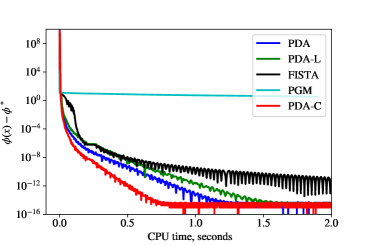
(a) $\phi(x)-\phi^{*}$

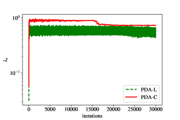
(b) $\lambda_{n}$ (or $\tau_{k}$)

Figure 1: Comparison of $\phi(x)-\phi^{*}$ and $\lambda_{n}$ (or $\tau_{k}$) for solving Problem 1 generated by the first way.

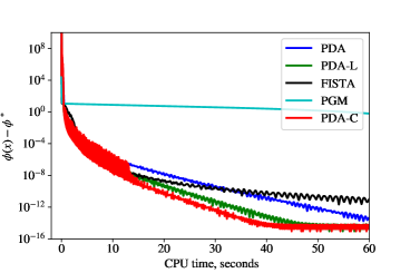
(a) $\phi(x)-\phi^{*}$.

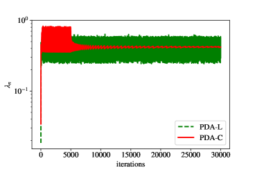
(b) $\lambda_{n}$ (or $\tau_{k}$)

Figure 2: Comparison of $\phi(x)-\phi^{*}$ and $\lambda_{n}$ (or $\tau_{k}$) for solving Problem 1 generated by the second way.

To illustrate how does the values $\phi(x_{n})-\phi^{*}$ ($\phi^{*}=\phi(\bar{x})$ with $(\bar{x},\bar{y})\in{\mathcal{S}}$) and $\lambda_{n}$ for PDA-C (or $\tau_{k}$ for PDA-L) change over iterations, we give two convergence plots for the maximum number of iterations set at 30,000. From the results shown in Fig. 1 and 2, primal-dual methods show better performance for the instances of Problem 1, though they require a tuning the parameter $\beta$.

For the tested problems, PDA-C needs to correct less that 20 times linesearch, so PDA-C with $\delta=0.62$ is more efficient than PDA-L. The advantage of PDA-C is a larger interval for possible step size $\lambda_{n}$, see Fig.1 (b) and Fig.2 (b), which resulted from the smaller choice of $\delta$ and the larger value of $\alpha$.

Problem 2 (Min-max matrix game)

The second problem is the following min-max matrix game

$$\min_{x\in\Delta_{n}}\max_{y\in\Delta_{m}}\left\langle Kx,y\right\rangle,$$ (64)

where $x\in\mathbb{R}^{n}$, $y\in\mathbb{R}^{m}$, $K\in\mathbb{R}^{m\times n}$, and $\Delta_{m}$, $\Delta_{n}$ denote the standard unit simplices in $\mathbb{R}^{m}$ and $\mathbb{R}^{n}$ respectively.

The variational inequality formulation of (64) is:

$$\left\langle F(z^{*}),z-z^{*}\right\rangle+G(z)-G(z^{*})\geq 0\quad\forall z\in Z,$$

where

$$Z=\mathbb{R}^{n}\times\mathbb{R}^{m},\quad z=\binom{x}{y},\quad F=\begin{bmatrix}0&K^{*}\\ -K&0\end{bmatrix},\quad G(z)=\delta_{\Delta_{n}}(x)+\delta_{\Delta_{m}}(y).$$

For a comparison we use a primal-dual gap (PD gap) as in M_PDA , which can be easily computed for a feasible pair $(x,y)$, defined as

$$G(x,y):=\max_{i}(Kx)_{i}-\min_{j}(K^{*}y)_{j}.$$

We use an auxiliary point (see modified-FB ) to compute the primal-dual gap for Tseng’s method FBF, as its iterates may be infeasible. The initial point in all cases is chosen as $x_{0}=\frac{1}{n}(1,\cdots,1)$ and $y_{0}=\frac{1}{m}(1,\cdots,1)$. We use the algorithm from projections to compute projection onto the unit simplex. For PDA we set $\tau=\sigma=\frac{1}{\|K\|}$, which we compute in advance. The input data for FBF and PEGM with linesearch are taken the same as in Proximal-extrapolated . For PDA-L and PDA-C we set $\beta=1$ (the same as $\tau=\sigma$ in PDA) and for PDA-C we set $\hat{n}=40,000$. Since PDA-C with $\delta=1$ performs well than smaller $\delta$ for the min-max matrix game, we apply PDA-C with $\delta=1$ to testify.

We consider four differently generated samples of the matrix $K\in{\mathbb{R}}^{m\times n}$ with $seed=100$ as in M_PDA :

• $m=100$, $n=100$. All entries of $K$ are generated independently from the uniform distribution in $[-1,1]$;

• $m=100$, $n=100$. All entries of $K$ are generated independently from the normal distribution ${\mathcal{N}}(0,1)$;

• $m=500$, $n=100$. All entries of $K$ are generated independently from the normal distribution ${\mathcal{N}}(0,10)$;

• $m=100$, $n=200$. All entries of $K$ are generated independently from the uniform distribution in $[0,1]$.

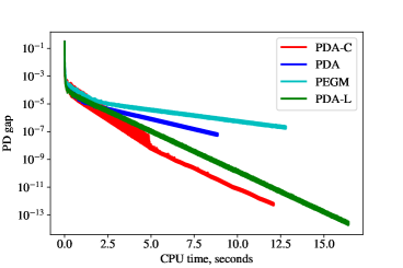
(a) Example 1.

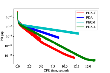
(b) Example 2.

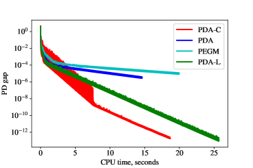
(c) Example 3.

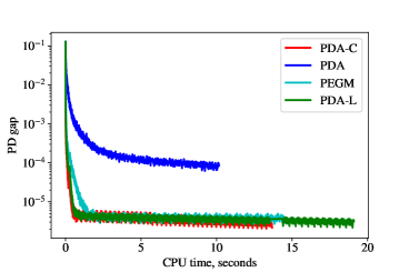
(d) Example 4.

Figure 3: Comparison of PD gap for solving Problem 2 within 100,000 iterations.

For every case we report the computing time (Time) measured in seconds, and show the primal-dual gap vs the computing time. The results are presented in Fig. 3. The execution time of all iterations for PDA is the lowest, PDA-C is slightly more than PDA, and PDA-L is about 2 times more expensive than PDA. From Fig. 3, PDA-L and PDA-C show better performance than PDA for the instances of Problem 2. Furthermore, we notice that PDA-C can be better than PDA-L.

Problem 3 (Nonnegative least square problem)

We are interested in the following problem

$$\min_{x>0}\phi(x):=\frac{1}{2}||Kx-b||^{2}$$

or in a primal-dual form

$$\min_{x\in\mathbb{R}^{n}}\max_{y\in\mathbb{R}^{m}}g(x)+\langle Kx,y\rangle-f^{*}(y),$$ (65)

where $f(p)=\frac{1}{2}||p-b||^{2}$, $f^{*}(y)=\frac{1}{2}||y||^{2}+(b,y)=\frac{1}{2}||y+b||^{2}-\frac{1}{2}||b||^{2}$, $g(x)=\delta_{\mathbb{R}^{n}_{+}}(x)$.

We consider two real data examples from the Matrix Market library One is “WELL1033”: sparse matrix with $m=1033,n=320$, another is “ILLC1033”: sparse matrix with $m=1033,n=320$. For all cases the entries of vector $b\in{\mathbb{R}}^{m}$ are generated independently from ${\mathcal{N}}(0,1)$.

To apply FISTA, we define $h(x)=f(Kx)=\frac{1}{2}||Kx-b||^{2}$ for Problem 3, then $\nabla h(x)=K^{*}(Kx-b)$. Since $f^{*}$ is strongly convex, in addition to PDA, PDA-L, and FISTA, we include in our comparison APDA, APDA-L and APDA-C. We apply APDA-L to the primal-dual form (65) and APDA-C to the symmetry of (65), namely,

$$f^{*}(y)=\delta_{\mathbb{R}^{n}_{+}}(y),~{}~{}~{}g(x)=\frac{1}{2}||x+b||^{2}-\frac{1}{2}||b||^{2}.$$

We take parameter of strong convexity as $\gamma=1/2$. For PDA, APDA, and FISTA we compute $\|K\|$ and set $\tau=\sigma=\frac{1}{\|K\|}$, $\alpha=\frac{1}{\|K\|^{2}}$. For PDA-L and PDA-C we set $\beta=1$ (the same as $\tau=\sigma$ in PDA) and for PDA-C we set $\hat{n}=5000$. Since $\lambda_{n}\rightarrow 0$ from Lemma 5, we set $\phi_{n}\equiv 1$ for APDA-C in this section. The initial points are $x_{0}=(0,\cdots,0)$ and $y_{0}=Kx_{0}-b=-b$.

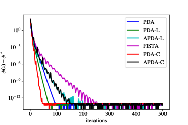
(a) $\phi(x)-\phi^{*}$

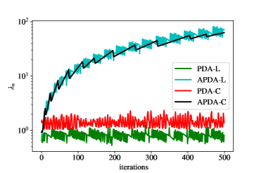
(b) $\lambda_{n}$(or $\beta_{n-1}\lambda_{n}$, $\tau_{k}$)

Figure 4: Comparison of $\phi(x)-\phi^{*}$ and $\lambda_{n}$(or $\beta_{n-1}\lambda_{n}$, $\tau_{k}$) for solving Problem 3 with “WELL1033”.

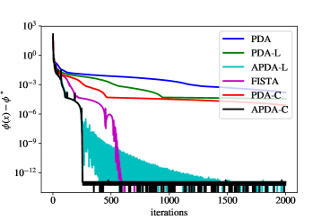
(a) $\phi(x)-\phi^{*}$

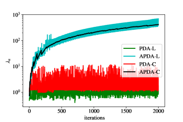
(b) $\lambda_{n}$(or $\beta_{n-1}\lambda_{n}$, $\tau_{k}$).

Figure 5: Comparison of $\phi(x)-\phi^{*}$ and $\lambda_{n}$(or $\beta_{n-1}\lambda_{n}$, $\tau_{k}$) for solving Problem 3 with “ILL1033”.

We illustrate the plots of $\phi(x_{n})-\phi^{*}$ and $\lambda_{n}$ from PDA-C (or $\beta_{n-1}\lambda_{n}$ from APDA-C, $\tau_{k}$ from PDA-L) change over iterations. From the results shown in Fig. 4 and 5, we observe that PDA-C with $\delta=0.62$ and PDA-L show better performance for the case “WELL1033”, while APDA-C and APDA-L for the case “ILL1033”. It is interesting to highlight that sometimes non-accelerated methods can be better than their accelerated variants for the well problems.

6 Conclusions

In this work, we have presented a primal-dual algorithm with correction and explored its acceleration. Firstly, the proposed PDA-C allows us to avoid the evaluation of the operator norm. Secondly, we have presented a prediction-correction strategy to estimate step sizes, which may results in larger step sizes. In practice, the correction step is conducted infrequently as only a weak condition needs to satisfy. Finally, we have proved convergence and established convergence rate, for PDA-C and its accelerated version.

Notice that only a very weak condition needs to check in the correction, and the correction step is not necessary to arrive termination conditions for some problems. Whether do the proposed PDA converge without correction? For $\delta\in]0,\frac{\sqrt{5}-1}{2}]$, whether there are any (larger) $\alpha>0$ such that the proposed PDA is convergent? We leave these as interesting topics for our future research.

References

(1)Arrow, K. J., Hurwicz, L. and Uzawa, H.: Studies in Linear and Non-Linear Programming, Stanford Mathematical Studies in the Social Sciences, II, Stanford University Press, Stanford, CA (1958)
(2)
Antipin, A.S.:
On a method for convex programs using a symmetrical modification of the Lagrange function.
Ekonomika i Matematicheskie Metody, 12(6), 1164–1173 (1976)
(3)
Arrow, K. J., Hurwicz, L., and Uzawa, H. Studies in linear and non-linear programming. Stanford University Press (1958)
(4)
Bauschke, H.H., Combettes, P.L.:
Convex Analysis and Monotone Operator Theory in Hilbert Spaces.
Springer Berlin, New York (2011)
(5)
Beck, A., Teboulle, M.:
A fast iterative shrinkage-thresholding algorithm for linear inverse problems.
SIAM J. Imgaging Sci. 2(1), 183–202 (2009)
(6)
Bertsekas, D.P., Gafni, E.M.:
Projection methods for variational inequalities with applications to the traffic assignment problem.
Math. Prog. Study, 17, 139–159 (1982)
(7)
Burachik, R.S., Lopes, J.O., Svaiter, B.F.:
An outer approximation method for the variational inequality problem.
SIAM J. Control Optim. 43(6), 2071–2088 (2005)
(8)
Boyd, S., Parikh, N., Chu, E., Peleato, B., Eckstein, J.:
Distributed optimization and statistical learning via the alternating direction method of multipliers.
Found. Trends Mach. Learn. 3(1), 1–122 (2011)
(9)
Bo R.I., Csetnek, E.R.:
Forward-backward and Tseng’s type penalty schemes for monotone inclusion problems.
Set-Valued Var. Anal. 22, 313–331 (2014)
(10)
Bo R.I., Csetnek, E.R.:
An inertial forward-backward-forward primal-dual splitting algorithm for solving monotone inclusion problems.
Numer. Algor. 71, 519–540 (2016)
(14)
Chambolle, A., Pock, T.: A first-order primal-dual algorithm for convex problems with applications to imaging. J. Math. Imaging Vis., 40(1):120–145 (2011)
(15)
Douglas J., Rachford, H. H.: On the numerical solution of the heat conduction problem in 2 and 3 space variables, Trans. Amer. Math. Soc., 82, pp. 421–439 (1956)
(16)
Duchi, J., Shalev-Shwartz, S., Singer, Y., and Chandra, T.: Efficient projections onto the -ball for learning in high dimensions. In Proceedings of the 25th international conference on Machine learning, pp. 272–279 (2008)
(17)
Ekeland, I., Temam R.:
Convex Analysis and Variational Problems.
North-Holland, Amsterdam, Holland (1976)
(18) Facchinei, F., Pang, J.-S.:
Finite-Dimensional variational inequalities and complementarity problem.
Springer-Verlag, New York (2003)
(19)
He, B., Yuan, X.:
A class of ADMM-based algorithms for multi-block separable convex programming.
Comput. Optim. Appl. 70(3), 791–826 (2018)
(20)
He, B., Yuan, X.: Convergence analysis of primal-dual algorithms for a saddle-point problem: from contraction perspective.
SIAM J. Imaging Sci., 5(1):119–149 (2012)
(21)
Iusem, A.N., Pérez, L.R.:
An extragradient-type algorithm for nonsmooth variational inequalities.
Optimization, 48, 309–332 (2000)
(22)
Korpelevich, G.M.:
The extragradient method for finding saddle points and other problem.
Ekonomika i Matematicheskie Metody, 12, 747–756 (1976)
(23)
Liu, Y., Xu, Y., Yin W.: Acceleration of primal-dual methods by preconditioning and simple subproblem procedures. https://arxiv.org/abs/1811.08937v2 (2018)
(25)
Malitsky, Y.V., Semenov, V.V.:
An extragradient algorithm for monotone variational inequalities.
Cybern. Syst. Anal. 50, 271–277 (2014)
(26)
Malitsky, Y., Pock, T.: A first-order primal-dual algorithm with linesearch. SIAM J. Optimiz., 28(1):411-432 (2018)
(27)
Malitsky Y . Golden ratio algorithms for variational inequalities.
https://arxiv.org/abs/1803.08832 (2019)
(28)
Noor, M.A.:
Modified projection method for pseudomonotone variational inequalities.
Appl. Math. Lett. 15, 315–320 (2002)
(29)
Nesterov, Y.:
A method of solving a convex programming problem with convergence rate .
Soviet Mathematics Doklady, 27(2), 372–376 (1983)
(30)
Nesterov, Y.:
Introductory lectures on convex optimization: A basic course.
Kluwer Academic Publishers, Boston (2004)
(31)
Nesterov, Yu.: Gradient methods for minimizing composite objective function. Technical report, CORE DISCUSSION PAPER
(2007)
(32)
Nemirovski, A.:
Prox-method with rate of convergence for variational inequalities with Lipschitz continuous monotone operators and smooth convex-concave saddle point problems.
SIAM J. Optim. 15, 229–251 (2004)
(33)
Pock, T., and Chambolle, A.: Diagonal preconditioning for first order primal-dual algorithms in convex optimization. In Computer Vision (ICCV), 2011 IEEE
International Conference, IEEE, pp. 1762–1769 (2011)
(34)
Popov, L. D.: A modification of the Arrow-Hurwitz method of search for saddle points, Mat. Zametki, 28, pp. 777–784 (1980)
(35)
Tseng, P.:
A modified forward-backward splitting method for maximal monotone mapping.
SIAM J. Control Optim. 38, 431–446 (2000)
(36)
Yang J., Liu H.:
A modified projected gradient method for monotone variational inequalities.
J. Optim. Theory Appl. 179(1), 197–211 (2018)
(37)
Zhang, X., Burger, M., Osher, S.: A unified primal-dual algorithm framework based on bregman iteration. J. Sci. Comput. 46(1):20–46 (2011)
(38)Zhu, M., Chan, T. F.: An efficient primal-dual hybrid gradient algorithm for total variation image restoration, CAM Report 08–34, UCLA, Los Angeles, CA (2008)