$\mathbb{Z}_{N}$ gauge theories coupled to topological fermions: QED₂ with a quantum-mechanical $\theta$ angle

Abstract

We present a detailed study of the topological Schwinger model [Phys. Rev. D 99, 014503 (2019)], which describes (1+1) quantum electrodynamics of an Abelian $U(1)$ gauge field coupled to a symmetry-protected topological matter sector, by means of a class of $\mathbb{Z}_{N}$ lattice gauge theories. Employing density-matrix renormalization group techniques that exactly implement Gauss’ law, we show that these models host a correlated topological phase for different values of $N$, where fermion correlations arise through inter-particle interactions mediated by the gauge field. Moreover, by a careful finite-size scaling, we show that this phase is stable in the large-$N$ limit, and that the phase boundaries are in accordance to bosonization predictions of the $U(1)$ topological Schwinger model. Our results demonstrate that $\mathbb{Z}_{N}$ finite-dimensional gauge groups offer a practical route for an efficient classical simulation of equilibrium properties of electromagnetism with topological fermions. Additionally, we describe a scheme for the quantum simulation of a topological Schwinger model exploiting spin-changing collisions in boson-fermion mixtures of ultra-cold atoms in optical lattices. Although technically challenging, this quantum simulation would provide an alternative to classical density-matrix renormalization group techniques, providing also an efficient route to explore real-time non-equilibrium phenomena.

I Introduction

One of the greatest achievements of condensed-matter physics in the last century has been the classification of states of matter by the phenomenon of spontaneous symmetry breaking landau_sb . This has lead to a universal description of a wide variety of quantum states of matter, and phase transitions thereof, through the identification of effective field theories involving local order parameters. However, after the discovery of integer quantum Hall states iqhe_exp ; qhe_invariant , it was soon realized that important quantum phases that are not contained in the Ginzburg-Landau symmetry breaking paradigm can exist. In particular, the description of these new states of matter requires the introduction of non-local order parameters, and the interplay of certain mathematical tools of topology, such as topological invariants, with global protecting symmetries of the microscopic models. Two states that show different topological invariants cannot be adiabatically connected, even if they share the same symmetry. Instead, quantum phase transitions induced by symmetry-preserving couplings must occur, which cannot be accounted for by the symmetry-breaking principle. These so-called symmetry protected topological (SPT) phases lie at the focus of current research in condensed matter, and have interesting connections to high-energy physics. Since the pioneering work of F.D.M. Haldane haldane_spt , C. Kane and E. Mele kane_mele_z2 , a variety of SPT phases beyond the integer quantum Hall states have been identified. These phases arise in different symmetry classes and dimensionalities, such as the so-called topological insulators and superconductors kane_rmp_ti ; qi_rmp_ti , and some of them have already been realized experimentally tis_exp .

In analogy to the quantum Hall effect, where the introduction of inter-particle interactions can lead to strongly-correlated phases with exotic properties fqhe_exp (e.g. excitations with fractional statistics fqhe_laughlin ), a problem of current interest in the community is to understand the fate of this variety of SPT phases in the presence of interactions corr_ti . The typical models considered so far have mostly focused on instantaneous interactions of various ranges (e.g. screened Coulomb interactions, or truncated versions thereof, such as Hubbard-type couplings). More recently, some studies spt_gauge ; spt_schwinger ; gonzalez_cuadra_18 ; gonzalez_cuadra_19 have started to explore strongly-correlated SPT phases with inter-particle interactions that are carried by auxiliary fields locally coupled to the matter sector, avoiding in this way the action at a distance of effective models with instantaneous interactions. This leads to interesting scenarios with intertwined topological phases that simultaneously display symmetry breaking, as characterised by a local order parameter, and topological symmetry protection, as described by a non-zero topological invariant gonzalez_cuadra_18 ; gonzalez_cuadra_19 . This more general framework of interacting SPT phases also allows one to explore models where interparticle interactions are carried by gauge bosons, and constrained by imposing invariance under local gauge symmetries spt_gauge ; spt_schwinger . These microscopic models parallel the use of gauge theories in the fundamental interactions of particle physics YM_non_abelian ; qft_book , and are particularly interesting in the context of non-perturbative effects in high-energy physics qcd_confinement .

As outlined above, the study of SPT phases in condensed matter originated with the study of two- and three-dimensional topological insulators kane_rmp_ti ; qi_rmp_ti . These phases of matter can be understood as lower-dimensional counterparts of the so-called domain-wall fermions in lattice gauge theories dw_kaplan ; kaplan_review ; dw_fermions . In this context gattringer_lang_book ; kogut_review , non-perturbative aspects of chiral gauge theories are studied on the boundary of a (4+1)-dimensional lattice, such that the existance of chiral fermions can be connected to a non-zero topological invariant and the so-called topological edge states. In the domain-wall fermion approach to LGTs gattringer_lang_book , one introduces an auxiliary synthetic dimension, such that Dirac fermions with a well-defined chirality become exponentially localised within the boundaries of this auxiliary dimension, and interact via local couplings to the Abelian or non-Abelian gauge fields. We note that one is interested only in the physics that takes place on such boundaries, and not along the auxiliary dimension, and may decide to place the gauge fields only along the boundary. In the study of correlated SPT phases interacting via gauge bosons, the auxiliary dimension represents the physical bulk of the material. Therefore, gauge fields must thus also be defined within the bulk, and be minimally coupled to the bulk matter according to gauge-symmetry constraints. This difference becomes relevant for the (1+1) model studied in this work, as one can define a gauge field theory in the 1D bulk, but the zero-dimensional edges cannot encompass a quantum field theory with gauge symmetry.

A well-studied gauge theory in low dimensions is the so-called Schwinger model schwinger_model , which describes quantum electrodynamics of relativistic fermions on the line. The Schwinger model can be considered as a paradigmatic toy model that unveils certain fundamental aspects that also play a role in higher-dimensional gauge theories, as well as interesting aspects that arise only as a consequence of the low dimensionality. One finds several peculiarities already at the classical level, since magnetic fields and photons do not exist, and static charges generate electric fields that do not decay with the distance. Upon quantization, one encounters the phenomenon of chiral symmetry breaking  as the massless fermions pair and only massive excitations are found schwinger_model . This model has also played a key role in our current understanding of anomalies anomalies_schwinger , and the importance of the so-called topological angles in the degeneracy of vacua theta_angle_schwinger . In this manuscript, we shall be concerned with the massive Schwinger model, which describes massive relativistic fermions coupled via the one-dimensional electromagnetic field massive_schwinger_shielding ; massive_schwinger_theta , and its various lattice discretizations.

More specifically, in Ref. spt_schwinger , we introduced an alternative discretization of the continuum Schwinger model schwinger_model leading to the topological Schwinger model: an Abelian gauge theory that regularizes quantum electrodynamics in (1+1) dimensions (QED₂), and describes the coupling of the electric field to a fermionic SPT matter sector. In contrast to the standard discretization of the massive Dirac fields, where one explicitly breaks translational invariance by using a staggered mass ham_lgt , we chose to break the symmetry by a dimerized tunnelling. In the continuum limit, such a tunnelling leads to Dirac fermions with a topological mass, and a matter sector that can be described as a fermionic SPT phase with a non-vanishing topological invariant and localised edge states spt_schwinger . Using bosonization, we showed that the coupling of this topological matter sector to the Abelian gauge field generates a quantum-mechanical vacuum $\hat{\theta}$ angle, which is no longer fixed by an external background electric field massive_schwinger_shielding ; massive_schwinger_theta , but depends on the fermionic density on the edge states. We also used the bosonized theory to predict fundamental differences between the standard Schwinger model with a background $\theta=\pi$ angle, and this topological Schwinger model with a quantum-mechanical $\hat{\theta}$ angle spt_schwinger . Let us note that, in the context of (3+1) time-reversal topological insulators, the response of the material to external electromagnetic fields can be described by an effective gauge field theory with an adiabatic axion field $\theta(\bm{x},t)$ axion_ti , which becomes a vacuum $\theta$ angle when the axion field is homogeneous and constant, and is related to the topological invariant characterising the matter sector kane_rmp_ti ; qi_rmp_ti . Our bosonization results can be understood as a lower-dimensional counterpart of the axion vacuum angle, which neatly captures the bulk-edge correspondence. Instead of relating the vacuum $\theta$ angle to a topological invariant axion_ti , the bosonization approach upgrades this angle to a quantum-mechanical operator $\hat{\theta}$ that depends on the topological edge-state operators, and may have its own dynamics beyond the adiabatic regime.

In order to test these bosonization predictions, we performed a numerical study based on the density-matrix renormalization group (DMRG) spt_schwinger . Instead of exploring the compact $U(1)$ LGT, one may employ the finite-dimensional gauge groups $\mathbb{Z}_{N}$ for different values of $N$ hamiltonian_z_n_gauge ; zn_presentation ; alternative_z_n_gauge ; alternative_z_n_gauge ; zn_study . In Ref. spt_schwinger , we explored in detail the $\mathbb{Z}_{3}$ LGT with a topological matter sector, showing that the above bosonization predictions qualitatively capture the physics already at $N=3$. We found that the phase diagram, as a function of the tunnelling dimerization and the gauge coupling, contains a wide region with a correlated SPT phase, where the correlations are induced by the fermion-fermion interactions mediated by the gauge field. This SPT phase is surrounded by other phases that also appear in the standard Schwinger model at $\theta=\pi$, namely a fermion condensate and a confined phase massive_schwinger_shielding ; massive_schwinger_theta . We found no adiabatic path connecting these phases, but instead Ising-type quantum phase transitions take place. In this work, we perform a quantitative benchmark of the bosonization predictions by exploring larger values of $N$, and performing a scaling analysis to extract large-$N$ limit zn_study , where one expects to recover the predictions for the compact $U(1)$ LGT. We provide a more detailed description of the numerical DMRG simulations presented in spt_schwinger , and present new numerical results that provide further information about the properties of the topological Schwinger model. In particular, we quantitatively confirm the bosonization predictions about the precise location of the critical lines at weak couplings. This quantitative analysis proves that the $\mathbb{Z}_{N}$ finite-dimensional gauge groups offer a practical route for an efficient classical simulation of equilibrium properties of QED₂ with topological fermions.

Let us note that LGTs are not mere computational tools, but may also become realized in experimental systems far from the high-energy-physics domain. In particular, some of the discretized LGTs could be implemented with highly-tunable quantum systems  QS_cold_atoms ; QS_trapped_ions in the low-energy domain: quantum simulators (QSs) feynman_qs ; qs_goals . These QSs have the potential of becoming an alternative to Monte-Carlo-based simulation of LGTs, addressing non-perturbative questions about the model using quantum-mechanical hardware, and evading in this way current numerical limitations regarding real-time observables, or the occurrence of the fermion sign problem. In Ref. spt_schwinger , we outlined that it should be possible to implement the aforementioned topological Schwinger model using ultra-cold atoms in optical lattices. Building on previous proposals for the quantum simulation of LGTs qs_LGT_review , we describe in this manuscript a concrete and detailed proposal for the quantum simulation of this type of LGTs coupled to a topological matter sector. In particular, we show how to combine spin-changing collisions in boson-fermion mixtures of ultra-cold atoms, and Floquet engineering by periodic drivings, in order to realize the desired topological Schwinger model.

This paper is stuctured as follows. In Sec. II, we start by reviewing the properties of standard Schwinger model in the continuum, and describe its discrete lattice version through the Kogut-Susskind Hamiltonian approach employing staggered fermions ham_lgt . This discussion allows us to introduce in a natural way the alternative discretization that will give rise to a topological matter sector, and the use of $\mathbb{Z}_{N}$ gauge groups as a proxy of the Abelian $U(1)$ gauge fields. In Sec. III, we start by reviewing some results obtained in Ref.spt_schwinger for the $\mathbb{Z}_{3}$ LGT coupled to a topological matter sector, and describe the corresponding phase diagram. Then, by using DMRG, we present new results on the scaling of the block entanglement entropies, providing accurate estimates of the universality classes of the critical lines. We extract the central charges of the underlying conformal field theories for the critical lines, and show that the $c=1$ massless Dirac fermion of the non-interacting model splits into a couple of $c=1/2$ massless Majorana fermions as soon as the gauge coupling $g$ is switched on. Moreover, we consider the cases when the gauge fields belong to the groups $\mathbb{Z}_{N}$ with $N=5$ and $N=7$, performing a careful finite-size scaling in the thermodynamic limit of two order parameters for extracting the position of the critical lines and their universality classes. In addition, we study the scaling with $N\to\infty$ of the critical points for accessing the $U(1)$ limit of the $\mathbb{Z}_{N}$ topological Schwinger model, and compare the numerical large-$N$ results with the bosonization predictions for the $U(1)$ LGT. In Sec. IV, we introduce a scheme based on spin-changing collisions and periodic lattice modulations, sometimes referred to as Floquet engineering floquet_cold_atoms , for the realization of the topological Schwinger model in a Bose-Fermi mixture of ultra-cold atoms in a 1D optical lattice. This scheme provides a promising, albeit challenging, route for a future experimental quantum simulation. Finally, Sec. V contains concluding remarks and gives outlook on future work.

II The topological Schwinger model

II.1 Continuum Schwinger model with a $\theta$ angle

In this section, we start by reviewing the continuum massive Schwinger model massive_schwinger_shielding ; massive_schwinger_theta , which describes the interaction of a massive Dirac fermion interacting with the electromagnetic field. In a (1+1)-dimensional Minkowski spacetime with coordinates $x^{\mu}$, $\mu\in\{0,1\}$ (i.e. $x=(t,{\rm x})$), and after setting $\hbar=c=1$, the Lagrangian density that dictates the dynamics of the fermionic and gauge fields is given by

$$\mathcal{L}_{{\rm S}}(m,g)=\overline{\Psi}({\rm i}\gamma^{\mu}(\partial_{\mu}+{\rm i}gA_{\mu})-m){\Psi}-\textstyle\frac{1}{4}F^{\mu\nu}F_{\mu\nu},$$ (1)

where $\partial_{\mu}=\partial/\partial x^{\mu}$, $A_{\mu}(x)=\eta_{\mu\nu}A^{\nu}(x)$, and we use the repeated-indexes summation criterion with Minkowski’s metric $\eta={\rm diag}(1,-1)$. In the expression above, we have introduced the Dirac matrices satisfying the anti-commutation relations $\{\gamma^{\mu},\gamma^{\nu}\}=2\eta^{\mu\nu}$. In (1+1) dimensions, the Dirac matrices can be represented in terms of Pauli matrices, and our choice is $\gamma^{0}=\sigma^{y}$, and $\gamma^{1}={\rm i}\sigma^{z}$. We have also introduced $\overline{\Psi}(x)=\Psi^{\dagger}(x)\gamma^{0}$, and the (bare) coupling $g$ of the fermion current to the gauge field with a Faraday tensor $F_{\mu\nu}=\partial_{\mu}A_{\nu}-\partial_{\nu}A_{\mu}$. With this notation, the fields have the classical mass (energy) dimensions $d_{\psi}=1/2$ and $d_{A_{\mu}}=0$, while the mass and gauge coupling have $d_{m}=d_{g}=1$.

The Schwinger model is the simplest tractable QFT that captures some of the most significant non-perturbative effects displayed by non-Abelian gauge theories in higher dimensions. In the massless limit $m=0$, it was solved exactly by J. Schwinger schwinger_model , who showed that the spectrum can be described by non-interacting bosons with a mass proportional to the coupling strength. In this massless limit, single-fermion excitations do not appear in the spectrum, but only massive neutral quasiparticles composed of bound fermion-antifermion pairs. This is known as fermion trapping in the high-energy context massive_schwinger_shielding , and it is reminiscent of exciton formation in condensed matter exciton_formation_theory . In this later context, electrons and holes are attracted by the electromagnetic forces, forming bound states and leading a neutral bosonic quasi-particle. There are, however, also clear differences due to the relativistic nature of the fermions and the peculiarities of the Coulomb force in such reduced dimensions.

The Schwinger model also provides a neat framework for understanding important properties that are absent in classical electrodinamics, such as the chiral anomaly schwinger_anomaly , or the so-called vacuum $\theta$ angle, which modifies the Lagrangian as

$$\mathcal{L}_{{\rm S}}(m,g)\to\mathcal{L}_{{\rm S}}(m,g,\theta)=\mathcal{L}_{{\rm S}}(m,g)+\frac{\theta}{2\pi}gF_{0,1}.$$ (2)

This vacuum $\theta$ angle is a c-number with a simple interpretation: it is proportional to an external background electric field, which is responsible for the the origin of the vacua degeneracy in the massless limit schwinger_theta_vacuum ; schwinger_theta_chiral . In the massive regime $m\neq 0$, the Schwinger model can be used to understand charge shielding via the string tension between two separate probe charges (i.e. screening of the long-range Coulomb force between static charges) massive_schwinger_shielding , and string-breaking phenomena as the distance between the charges is increased beyond a certain value string_breaking . Moreover, the degeneracy with respect to the $\theta$ angle is lifted, and one finds that for $\theta=\pi$ there is a continuous quantum phase transition between the confined phase with fermion trapping, and a distinct symmetry-broken phase with a so-called fermion condensate massive_schwinger_theta , which is reminiscent of an exciton condensate from a condensed-matter perspective.

II.2 Lattice discretization of the Schwinger model

There are various numerical methods to unveil the above non-perturbative phenomena, and benchmark the analytical predictions. These methods typically rely on a discretization of the fermionic and gauge fields on a lattice qcd_confinement , and we shall focus on the Kogut-Susskind Hamiltonian approach ham_lgt . Here, only the spatial coordinates are discretized into the sites of a chain $\Lambda_{\ell}=\{{\rm x}:{\rm x}/a\in\mathbb{Z}_{N_{s}}\}$, where $a$ is the lattice spacing, and $N_{s}$ is the number of lattice sites. By writing ${\rm x}=na$ for $n\in\mathbb{Z}_{N_{s}}$, the matter sector of Dirac fermions can be represented by the so-called staggered fermions defined on the lattice sites $\Psi({\rm x}),\overline{\Psi}({\rm x})\to c_{n}^{\phantom{\dagger}},c^{\dagger}_{n}$, such that $\{c_{n}^{\phantom{\dagger}},c_{m}^{\dagger}\}=\delta_{n,m}/a$, which have an alternating staggered mass $m_{\rm s}(-1)^{n}$ depending on the parity of the site.

The gauge field sector, in the temporal gauge $A_{0}=0$, can be represented by rotor-angle operators (i.e. compact QED) living on the links of the lattice, and fulfilling $[L_{n},\Theta_{m}]=-{\rm i}\delta_{n,m}$. Here, the angle operators are related to the gauge field $\Theta_{n}=agA_{1}({\rm x})$ at ${\rm x}=(n+\textstyle\frac{1}{2})a$, while the rotors correspond to angular-momentum operators related to the electric field $L_{n}=E({\rm x})/g=F_{01}({\rm x})/g$. In this gauge, and using Schwinger’s prescription for gauge-invariant point-split operators $\bar{\Psi}({x}+\epsilon)\Psi({x})\to\bar{\Psi}({x}+\epsilon){\rm e}^{-{\rm i}g\int_{{x}}^{{x}+\epsilon}{\rm d}x^{\mu}A_{\mu}(x)}\Psi({x})$ schwinger_ps_gauge , also known as the Peierls’ substitution in condensed matter, the continuous-time Hamiltonian LGT for the standard massive Schwinger model becomes

$$H_{{\rm S}}\!=a\!\sum_{n=1}^{N_{s}}\!\left(\!\frac{-1}{2a}\!\left({\rm i}c_{n}^{{\dagger}}U_{n}^{\phantom{\dagger}}c_{n+1}^{\phantom{\dagger}}+{\rm H.c.}\!\right)\!+m_{\rm s}(-1)^{n}c_{n}^{{\dagger}}c_{n}^{\phantom{\dagger}}+\frac{g^{2}}{2}L_{n}^{2}\right)\!.$$ (3)

Here, we have introduced the link operators $U_{n}={\rm e}^{{\rm i}\Theta_{n}}$, which act as unitary ladder operators $U_{n}\ket{\ell}=\ket{\ell+1}$ in the basis of electric-flux eigenstates $L_{n}\ket{\ell}=\ell\ket{\ell}$ for $\ell\in\mathbb{Z}$.

Finally, we note that the aforementioned vacuum angle (2) can be introduced in this Hamiltonian formulation through a background electric field $E_{\rm ext}$ by substituting $L_{n}\to L_{n}+\theta/2\pi$, where $\theta=2\pi E_{\rm ext}/g$. With this notation, the lattice fields have the classical mass (energy) dimensions $d_{c}=1/2$ and $d_{L}=0$, while the mass and gauge coupling have $d_{m_{s}}=d_{g}=1$, and the lattice constant $d_{a}=-1$. In the continuum limit, one recovers Eq. (1) with the staggered mass playing the role of the Dirac mass $\mathcal{L}_{{\rm S}}(m_{\rm s},g,\theta)$.

II.3 Topological Schwinger model, quantum $\hat{\theta}$ angle, and $\mathbb{Z}_{N}$ lattice gauge theories

In our previous work spt_schwinger , we used an alternative discretization of the matter fields, which hosts an SPT phase where the fermions interact via the gauge field. This alternative discretization follows from noting that the staggered mass in Eq. (3) breaks translational invariance leading to a two-site unit cell. One may explore other discretizations with a two-site unit cell that also lead to massive fermions in the continuum limit. One possibility is to dimerize the tunnelings, as occurs in of the so-called Su-Schrieffer-Hegger model of polyacetylene in the static limit of a Peierls-dimerized chain ssh_polyacetylene ; polyacetylene_cont . The gauge-invariant version of these dimerized tunnelings leads to the lattice version of the topological Schwinger model

$$H_{t{\rm S}}\!=a\!\sum_{n=1}^{N_{\rm s}}\!\left(\!\frac{-1}{a}\left({\rm i}(1-\delta_{n})c_{n}^{{\dagger}}U_{n}^{\phantom{\dagger}}c_{n+1}^{\phantom{\dagger}}+{\rm H.c.}\!\right)\!+\frac{g^{2}}{2}L_{n}^{2}\right)\!,$$ (4)

where the dimerization vanishes for even sites $\delta_{2n}=0$, while it can be finite for odd sites $\delta_{2n-1}=\Delta$, and all the remaining operators and constants have been defined around Eq. (3). We note that the total number of sites $N_{s}$ should be even to respect inversion symmetry about the center of the chain.

As discussed in detail in Ref. spt_schwinger , the continuum limit of the matter sector polyacetylene_cont must be carefully reconsidered to correctly account for the possibility of having topological edge states and a non-zero topological invariant zak_phase ; berry_rmp . Here, we simply summarise the main result: for $\Delta\in(0,2)$, one recovers Eq. (1) in the continuum limit with a new term that depends on the fermion density of the topological edge states

$$\mathcal{L}_{t{\rm S}}=\mathcal{L}_{t{\rm S}}(\Delta/a,g)-\sum_{\eta={\rm R,L}}\epsilon_{\eta}|\chi_{\eta}({\rm x})|^{2}\eta^{\dagger}\eta^{\phantom{\dagger}}.$$ (5)

This continuum limit shows that the tunneling dimerization gives a non-zero mass $m=\Delta/a$ to the Dirac fermions, while the topological nature of the SPT phase is revealed by the topological edge states of energies $\epsilon_{\eta}$ and wavefunctions $\chi_{\eta}({\rm x})$, which are exponentially localised to the left- and right-most edges of the system. The bosonization of this continuum gauge theory must carefully account for the edge term, as it represents boundary charges that will change the boundary Gauss’ law: the electric field can be discontinuous due to the charge localised at the left and right interfaces due to the existence of topological edge states. These considerations spt_schwinger lead to a quantum-mechanical edge contribution to the vacuum $\theta$ angle, which becomes an operator

$$\hat{\theta}=\theta+\pi\left({\rm sign}(x){\rm L}^{\dagger}{\rm L}-{\rm sign}(x-N_{\rm s}a){\rm R}^{\dagger}{\rm R}\right).$$ (6)

Such a contribution is physically reasonable. If only one of the edge states is populated by a fermion, there is an effective polarization of the material with a topological origin. Considering the theory of electromagnetic fields in dielectric media, such a polarization will modify the electric field inside the material. If the external electric field is such that $\theta=\pi$, we see that the population of a single edge state, and the associated polarization, does effectively cancel the electric field seen by the fermions. In situations where there is no external electric field, the topological polarization of the media can self-generate a non-zero vacuum angle $\theta=\pi$.

This behaviour can certainly modify the phase diagram of the topological Schwinger model in comparison to the standard one. In particular, it leads to the phase diagram sketched in Fig. 1. As outlined above Eq. (5), the vertical axis at zero gauge coupling separates an SPT groundstate for dimerizations $\Delta\in(0,2)$ from a trivial band insulator for $\Delta<0$ or $\Delta>2$. As the gauge coupling $g$ is switched on, the fermions in the SPT phase start interacting via the gauge bosons, and acquire correlations. As a consequence of such interactions, the bare mass $m_{\rm s}=\Delta/a$ in Eq (5) gets renormalised, such that one finds quantum phase transitions separating the SPT phase from a topologically-trivial phase. As can be observed in Fig. 1, this phase corresponds to the confined phase (C) displaying massive neutral quasiparticles composed of bound fermion-antifermion pairs, which was mentioned in the introduction. At this point, since there are no longer edge states, the vacum angle becomes $\theta=\pi$, where another quantum phase transition towards a parity-breaking fermion condensate (FC) can take place massive_schwinger_theta . This is precisely the second critical line displayed in Fig. 1. We note that the bosonization allows for the analytical prediction of these two critical lines $\Delta=\Delta_{\rm c,1}(g)$, and $\Delta=\Delta_{\rm c,2}(g)$, at weak couplings

$$\Delta_{\rm c,1}(g)=-\frac{ga}{2\sqrt{\pi}}{\rm e}^{-\gamma},$$ (7)

where $\gamma\approx 0.5774$ is Euler’s constant, and

$$\Delta_{\rm c,2}(g)=-\frac{1}{3}ga,$$ (8)

together with their symmetric counterparts $\Delta=2-\Delta_{\rm c,1}(g)$, and $\Delta=2-\Delta_{\rm c,2}(g)$.

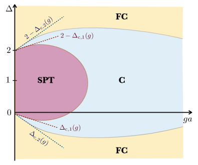
Figure 1: Phase diagram of the topological Schwinger model: The bosonization with the vacuum $\hat{\theta}$ operator (6) allows us to predict three distinct phases: a symmetry-protected topological (SPT) phase, corresponding to a correlated topological insulator, separated from a confined phase (C) through a continuous quantum phase transition. This confined phase is itself separated from a symmetry-broken fermion condensate (FC) by another continuous phase transition.

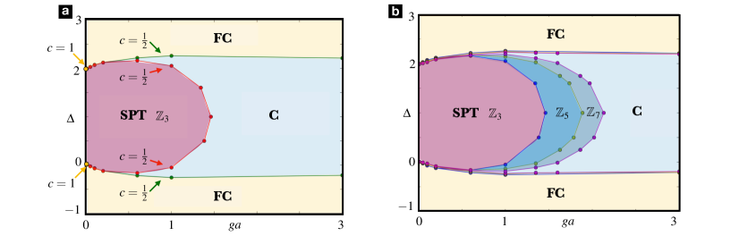
Figure 2: DMRG phase diagram for $\mathbb{Z}_{N}$ topological Schwinger models: (a) $\mathbb{Z}_{3}$ model, including the central charges of the critical lines. (b) $\mathbb{Z}_{5}$ and $\mathbb{Z}_{7}$ models, showing that the extension of the SPT phase grows as $N$ is increased.

Let us now introduce the discrete $\mathbb{Z}_{N}$ gauge group version of the topological Schwinger model spt_schwinger , which shall be used to benchmark the bosonization predictions of Fig. 1, and Eqs. (7)-(8). The Hamiltonian of $\mathbb{Z}_{N}$ LGT with topological matter reads

$$H^{\mathbb{Z}_{N}}_{t{\rm S}}\!=a\!\sum_{n=1}^{N_{s}}\!\left(\!\frac{-1}{a}\left({\rm i}(1-\delta_{n})c_{n}^{{\dagger}}\tilde{U}_{n}^{\phantom{\dagger}}c_{n+1}^{\phantom{\dagger}}+{\rm H.c.}\!\right)\!+\frac{g^{2}}{2}\tilde{L}_{n}^{2}\right)\!,$$ (9)

where the main difference with the Kogut-Susskind approach (4) is that the gauge fields are defined through the pair of link operators $\tilde{U}_{n},\tilde{V}_{n}$ that obey the $\mathbb{Z}_{N}$ algebra, fulfilling $\tilde{U}_{n}^{N}=\tilde{V}_{n}^{N}=\mathbb{I}$, and $\tilde{V}^{\dagger}_{n}\tilde{U}_{n}\tilde{V}_{n}={\rm e}^{{\rm i}2\pi/N}\tilde{U}_{n}$  alternative_z_n_gauge ; zn_presentation ; zn_study .

By using the electric-flux eigenbasis $\tilde{V}_{n}\ket{v}=v\ket{v}$ with $v\in\mathbb{Z}_{N}$ on each link, one can understand that the link operator $\tilde{U}_{n}$ acts as ladder operator that raises the electric flux by one quantum $\tilde{U}_{n}\ket{v}=\ket{v+1}$ in a cyclic way, i.e. $\tilde{U}_{n}\ket{N}=\ket{1}$. We note that these link operators can be defined in terms of the vector potential and the electric field $\tilde{U}_{n}={\rm exp}\{{\rm i}agA_{n}\}$, $\tilde{V}_{n}={\rm exp}\{{\rm i}\frac{2\pi}{N}\frac{E_{n}}{g}\}$. Accordingly, the $\mathbb{Z}_{N}$ algebra $[\tilde{U}_{n},\tilde{V}_{n}]={\rm e}^{{\rm i}2\pi/N}$ can be satisfied by imposing the usual canonical commutation relations on the gauge fields $[E_{n},A_{m}]={\rm i}\delta_{n,m}/a$, which have the correct continuum limit $[E(x),A(y)]={\rm i}\delta(x-y)$. Note also that the gauge-group condition $\tilde{U}_{n}^{N}=\tilde{V}_{n}^{N}=\mathbb{I}$ requires that the electric-flux eigenvalues of $\tilde{L}_{n}=E_{n}/g$ should span $\sigma(\tilde{L}_{n})=\{-\textstyle\frac{1}{2}(N-1),\cdots,\textstyle\frac{1}{2}(N-1)\}$. This yields $\sigma(\tilde{L}_{n})\to\mathbb{Z}$ in the large-$N$ limit, which corresponds to the spectrum of the rotor operator $L_{n}$ of the Kogut-Susskind approach  ham_lgt . In the same manner, the eigenvalues of the vector potential should lie in $\sigma(agA_{n})=\{-\pi(N-1)/N,\cdots,\pi(N-1)/{N}\}\to[-\pi,\pi]$, corresponding to the basis of the angle operator $\Theta_{n}$ in the Kogut-Susskind approach, and leading to compact QED₂. Therefore, one expects that the properties of compact QED₂ coupled to a topological matter sector can be reproduced by taking the large-$N$ limit of these $\mathbb{Z}_{N}$ LGTs.

Let us now address an important point of the lattice formulation. In the continuum, Gauss’ law and its interplay with bound topological charge at the edges is of paramount importance to determine the phase diagram. In the lattice, in order to take into account Gauss’s law, we introduce the operator

$$G_{n}=c_{n}^{\dagger}c_{n}+\frac{1}{2a}[(-1)^{n}-1]-\frac{1}{a}(\tilde{L}_{n}-\tilde{L}_{n-1}).$$ (10)

Accordingly, $\left|\psi\right>$ is a physical state if it satisfies the condition

$$G_{n}\left|\psi\right>=0\hskip 8.61108pt\forall n\in\{1,2,\cdots,N_{\rm s}\}.$$ (11)

This is a very important constraint that allows us to construct the physical Hilbert space of the $\mathbb{Z}_{N}$ model, as we will see in the following section.

III Density-matrix-renormalization-group simulations of the topological Schwinger model

III.1 $\mathbb{Z}_{3}$ topological Schwinger model

In this section, we start by reviewing the DMRG phase diagram for the simplest non-trivial case presented in spt_schwinger , the $\mathbb{Z}_{3}$ model (9) with three electric-flux levels on each link. This will serve us to set the common ground for the large-$N$ studies presented in the following sections. Before turning to larger values of $N$, we discuss new results concerning the entanglement spectroscopy entanglemnent_review for the critical lines of the $\mathbb{Z}_{3}$ LGT.

The different phases depicted in Fig. 1 can be characterised by two different observables: the electric-field order parameter, which can be defined as

$$\Sigma=\frac{1}{N_{s}}\sum_{n=1}^{N_{s}}\bra{\rm gs}E_{n}\ket{\rm gs}=\frac{g}{N_{s}}\sum_{n=1}^{N_{s}}\bra{\rm gs}\tilde{L}_{n}\ket{\rm gs}$$ (12)

and the topological correlator, namely

$$O_{-}=\frac{2}{N_{\rm s}}\sum_{n=1}^{N_{\rm s}/2}O^{(2n-1)}_{-},$$ (13)

where we sum over all odd sites of the chain the observables

$$O^{(n)}_{-}=\frac{3}{2}\bra{\rm gs}c_{n}^{\dagger}c_{n+1}^{\phantom{\dagger}}+c_{n+1}^{\dagger}c_{n}^{\phantom{\dagger}}\ket{\rm gs}+\rho_{n,n+1}-\frac{1}{2}(\rho_{n}+\rho_{n+1}).$$ (14)

Here, $\rho_{n}=\bra{\rm gs}c^{\dagger}_{n}c^{\phantom{\dagger}}_{n}\ket{\rm gs}$ are the densities of fermions, while $\rho_{n,n+1}=a\bra{\rm gs}c^{\dagger}_{n}c^{\phantom{\dagger}}_{n}c^{\dagger}_{n+1}c^{\phantom{\dagger}}_{n+1}\ket{\rm gs}$ represent the density-density correlations, and the site index $n$ must be odd. Such a topological correlator was introduced for the dimerized free-fermion model ssh_order_parameters , and used in Ref. spt_schwinger to map the phase diagram of the full $\mathbb{Z}_{3}$ topological Schwinger model.

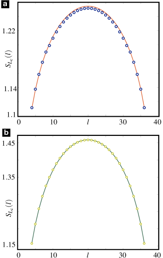
Figure 3: Block entanglement entropy of the $\mathbb{Z}_{3}$ model: (a) Scaling of the entanglement entropy of a subsystem of size $l$ on the critical point $\Delta=-0.162$ and $ga=0.6$. Through a logarithmic fit (15), it is possible to extract the central charge $c=0.506$. (b) Same as (a), but for $g=\Delta=0$.

By studying the behavior of these two quantities and performing a careful finite-size scaling analysis, we find the phase diagram of the the $\mathbb{Z}_{3}$ topological Schwinger model shown in Fig. 2 (a). The three different phases can be characterised as follows: i) the confined phase (C) with $\Sigma=0$ and $O_{-}<0$; ii) the fermion condensate (FC) with $\Sigma>0$ and $O_{-}<0$; iii) the symmetry-protected topological (SPT) phase with $\Sigma<0$ and $O_{-}>0$. We recall that the topological nature of SPT phase was revealed in spt_schwinger by showing the exact degeneracy in the entanglement spectrum ent_spectrum , and the existence of many-body edge states. In addition, from the scaling analysis, we estimated the values of the critical exponents $\beta$ and $\nu$, related to the two phase transitions FC-C and SPT-C. In both cases, we found $\beta=1/8$ and $\nu=1$, which correspond to the 2D Ising universality class.

We want now to confirm this finding by performing another independent analysis based on the scaling of the entanglement entropy. The entanglement entropy $S(\tilde{\rho}_{A})=-{\rm Tr}\left[\tilde{\rho}_{A}\log_{2}\left(\tilde{\rho}_{A}\right)\right]$ is defined for the reduced density matrix of a partition $A$ of our system $\tilde{\rho}_{A}={\rm Tr}_{B}{\ket{\rm gs}\bra{\rm gs}}$, where $B$ is the complement of $A$. According to conformal field theory (CFT) entan_entropy ; entanglement_entropy_calabrese_cardy , considering a subsystem A of size $l$ within the chain that has $L_{\rm c}=N_{\rm s}/2$ couples of sites, we expect to observe a logarithmic scaling of the block entanglement entropy if the system is at a quantum critical point

$$S_{L_{\rm c}}(l)=\frac{c}{6}\log_{2}\left[\frac{2L_{\rm c}}{\pi}\sin\left(\frac{\pi l}{L_{\rm c}}\right)\right]+s_{0},$$ (15)

where $s_{0}$ is a non-universal constant, and $c$ is the central charge of the corresponding CFT that governs the critical behavior. As shown in Fig. 3(a), we observe such a logarithmic scaling for the critical point $ga=0.6$ and $\Delta=-0.162$, from which it is possible to extract the central charge through a logarithmic fit. We obtain the value $c=0.506$, in agreement with the central charge of 2D Ising universality class $c=\textstyle\frac{1}{2}$. Interestingly, by switching off the gauge coupling $g=0$, we obtain the entanglement entropy of Fig. 3(b) at the critical point $\Delta=0$, which yields $c=1.059$ through the logarithmic fit. This result is in agreement with the expectation for the critical point of the dimerised free-fermion model, which can be described by the CFT of a massless Dirac fermion with $c=1$. Accordingly, the $c=1$ CFT of the non-interacting model splits into a couple of CFTs with $c=\textstyle\frac{1}{2}$, each of which controls the criticality of the SPT-C and C-FC quantum phase transitions, as depicted in Fig. 2 (a). We note that a similar splitting of a $c=1$ massless Dirac fermion into a couple of $c=1/2$ massless Majoranas has been recently observed in other models of correlated SPT phases with instantaneous Hubbard-type interactions instead of the gauge-mediated ones creutz_hubbard_ladder ; gross_neveu_wilson ; wilson_hubbard_matter .

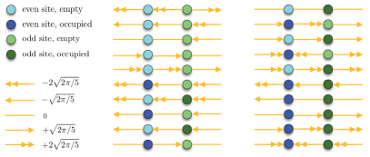
Figure 4: Basis of gauge-invariant Hilbert space for the $\mathbb{Z}_{5}$ model: taking into account Gauss’s law, we implement all possibile configurations of matter/antimatter fields on even/odd sites.

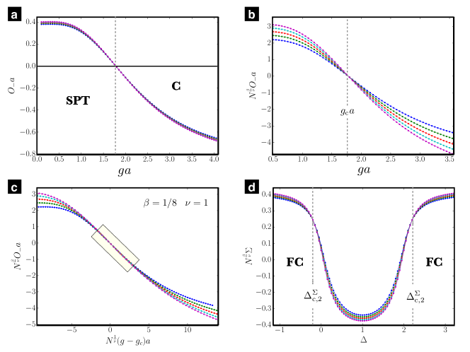
Figure 5: Observables and scaling relations for the $\mathbb{Z}_{5}$ topological Schwinger model: (a) Behavior of the topological correlator for $\Delta=0.5$ as a function of the gauge coupling constant g with $N_{s}=\left[40,50,60,70,80\right]$ sites (from blue ($40$) to purple ($80$)). (b) Scaling quantity $N^{\frac{\beta}{\nu}}O_{-}a$ of the topological correlator calculated for $\Delta=0.5$ as a function of the gauge coupling for various system sizes $N_{s}=\left[24,28,32,36,40\right]$ (from blue ($24$) to purple ($40$)). The crossing point of all curves allows us to determine the critical point separating the SPT and C phases $g_{c}a\approx 1.786$. (c) Universal scaling of the topological correlator with the critical exponents of the 2D Ising universality class $\beta=1/8$ and $\nu=1$: all the numerical curves for different system sizes $N_{s}$ collapse onto the same universal function $\lambda(x)$ in the shaded region. (d) Scaling quantity $N^{\frac{\beta}{\nu}}\Sigma$ of the electric field order parameter calculated for $ga=0.6$ as a function of the dimerization for various system sizes $N_{s}=\left[24,28,32,36,40\right]$ (from blue ($24$) to purple ($40$)). The crossing point of all curves allows us to determine the critical point separating the FC and C phases $\Delta^{\Sigma}_{c}\approx-0.193$ and $\Delta^{\Sigma}_{c}\approx 2.105$ in accordance with the symmetry around $\Delta=1$.

III.2 $\mathbb{Z}_{5}$ and $\mathbb{Z}_{7}$ topological Schwinger model

In this section, we consider the following question: what is the fate of the SPT phase as we increase the dimension of the gauge group symmetry $\mathbb{Z}_{N}$? To address this question, we perform DMRG simulations of our topological LGT (9) for larger values of $N$. We start by considering the $\mathbb{Z}_{5}$ case with five possible electric field levels on each link. In order to impose Gauss’ law (11) with the corresponding operator (10), one can directly build the gauge-invariant Hilbert space considering certain local configurations. For the $\mathbb{Z}_{5}$ gauge group, the basis of such local gauge-invariant configurations can be built by considering the two-site unit cell, with the corresponding gauge fields, as shown in Fig. 4. Through this local basis, we directly implement the gauge-invariant subspace in our DMRG code, reducing the complexity of the problem. We determine the ground-state of the system $\left|{\rm gs}\right>$ with open boundary conditions, working with up to $N_{s}=80$ sites and keeping 1200 DMRG-states at most. These values are large enough to ensure stability of our findings and small truncation errors.

First of all, in order to prove the presence of the SPT phase also in the $\mathbb{Z}_{5}$ model, we analyze the behavior of the topological correlator $O_{-}$ (13) for $\Delta=0.5$ as a function of the gauge coupling $g$. As shown in Fig. 5(a), we obtain a clear sign reversal of the correlator, a behavior that is qualitatively analogous to the transition from the topological phase ($O_{-}>0$) to the trivial one ($O_{-}<0$) observed in the $\mathbb{Z}_{3}$ case spt_schwinger . In order to extract the critical point, we can perform a finite-size scaling of the SPT order parameter $O_{-}$. In the $\mathbb{Z}_{3}$ model, the quantum phase transition SPT-C has critical exponents $\beta=1/8$ and $\nu=1$. Therefore, we can start to explore the critical behavior by assuming these values in the usual scaling relation

$$N_{\rm s}^{\frac{\beta}{\nu}}O_{-}=\lambda\left(N_{\rm s}^{\frac{1}{\nu}}(g-g_{\rm c})\right).$$ (16)

in which $\lambda(x)$ is a universal function. By fixing $\Delta=0.5$ and plotting the quantity $N_{\rm s}^{\beta/\nu}O_{-}$ as a function of $g$ for different values of $N_{s}$, we obtain the behavior of Fig. 5(b). From the scaling relation (16), it results that, for $g=g_{\rm c}$, the value $\lambda(0)$ becomes independent of the system size. Therefore, one should observe a crossing of the curves for different lengths precisely at the critical point. This is exactly the behavior displayed in Fig. 5(b), wich has a clear crossing that yields a value of the critical point of $g_{\rm c}\approx 1.786/a$. We now have to look at the numerical curves given by $N^{\beta/\nu}_{s}O_{-}$ versus $N^{1/\nu}_{s}(g-g_{c})$, for different $N_{s}$, which should all collapse onto the same universal function $\lambda(x)$ near the origin in case the critical exponents coincide with those of the 2D Ising model. This represents an important check for the values of the critical exponents, as clearly visible in Fig. 5(c).

Following this scheme, we can iterate this procedure i) for different values of $\Delta$ (horizontal lines in the plane $ga-\Delta$); ii) fixing a particular value of $g$ and varying the dimerization parameter $\Delta$ (vertical lines in the plane $ga-\Delta$). In this way we determine the critical values $\Delta^{O_{-}}_{\rm c,1}$ for the transitions SPT-C shown in Tab. 1, corresponding to the lower and upper parts of the critical line depicted in Fig. 1. As in the $\mathbb{Z}_{3}$ model, when the gauge coupling $g$ is sufficiently large, this transition is absent. We also observe the symmetry around $\Delta=1$.

We can now investigate the behavior of the FC-C transition by using the electric field order parameter $\Sigma$ (12). Assuming the same critical exponents $\beta=1/8$, $\nu=1$, we perform a finite-size scaling analysis with

$$N_{\rm s}^{\frac{\beta}{\nu}}\Sigma=\lambda\left(N_{\rm s}^{\frac{1}{\nu}}(\Delta-\Delta_{\rm c})\right),$$ (17)

Accordingly, for $g=0.6$, we obtain the plot in Fig. 5(d), which allows us to detect two critical points $\Delta_{\rm c,1}^{\Sigma}\approx-0.193$ and $\Delta_{\rm c},1^{\Sigma}\approx 2.105$, again symmetrical with respect to $\Delta=1$.

Also in this case, we can iterate this procedure to determine the critical points related to the transition FC-C for different values of $g$. The resulting values $\Delta^{\Sigma}_{\rm c,2}$ are shown in Table 1, and correspond to the to the lower and upper parts of the critical line depicted in Fig. 1.

$ga$	$\Delta_{\rm c,2}^{\Sigma}$	$\Delta_{\rm c,2}^{\Sigma}$	$\Delta_{\rm c,1}^{O_{-}}$	$\Delta_{\rm c,1}^{O_{-}}$
$0.01$	$0.005$	$1.998$	$0.007$	$1.996$
$0.05$	$-0.016$	$2.015$	$-0.015$	$2.018$
$0.10$	$-0.045$	$2.050$	$-0.042$	$2.045$
$0.20$	$-0.098$	$2.105$	$-0.096$	$2.097$
$0.60$	$-0.193$	$2.198$	$-0.162$	$2.170$
$1.00$	$-0.240$	$2.246$	$-0.136$	$2.140$
$1.35$	$-0.220$	$2.225$	$-0.025$	$2.025$
$3.00$	$-0.206$	$2.207$	$//$	$//$

Table 1: $\mathbb{Z}_{5}$ topological Schwinger model: critical values of $\Delta$ (related to the two transitions FC-C and SPT-C) obtained for different values of $g$. The numerical error is equal to $10^{-3}$.

We repeat all the numerical analysis also for the $\mathbb{Z}_{7}$ model (i.e. seven possible electric field levels on each link), observing the same behavior of the parameters $O_{-}$ and $\Sigma$. The critical values of both transitions SPT-C and FC-C are reported in Tab. 2. Putting together all these numerical results, we obtain the phase diagrams of the $\mathbb{Z}_{5}$ and $\mathbb{Z}_{7}$ topological Schwinger model shown in Fig. 2 with a comparison with the $\mathbb{Z}_{3}$ case. Here, one can observe that the extension of the SPT phase grows with $N$ while, simultaneously, the spacing between the critical lines becomes smaller. We can thus answer the question raised at the beginning of this section: as $N$ increases, the correlated SPT phase remains stable, and exits for a wider region of parameter space by displacing the confined phase towards larger values of the gauge coupling $g$. In the following section, we will address the large-$N$ limit, benchmarking the results for the $U(1)$ LGT by the bosonization predictions.

$ga$	$\Delta_{\rm c,2}^{\Sigma}$	$\Delta_{\rm c,2}^{\Sigma}$	$\Delta_{\rm c,1}^{O_{-}}$	$\Delta_{\rm c,1}^{O_{-}}$
$0.01$	$0.004$	$1.998$	$0.006$	$1.997$
$0.05$	$-0.010$	$2.009$	$-0.008$	$2.007$
$0.10$	$-0.030$	$2.032$	$-0.027$	$2.028$
$0.20$	$-0.085$	$2.089$	$-0.082$	$2.084$
$0.60$	$-0.178$	$2.181$	$-0.160$	$2.168$
$1.00$	$-0.228$	$2.231$	$-0.186$	$2.190$
$1.35$	$-0.215$	$2.218$	$-0.110$	$2.110$
$1.60$	$-0.212$	$2.212$	$-0.012$	$2.012$
$3.00$	$-0.190$	$2.190$	$//$	$//$

Table 2: $\mathbb{Z}_{7}$ topological Schwinger model: critical values of $\Delta$ (related to the two transitions FC-C and SPT-C) obtained for different values of $g$. The numerical error is equal to $10^{-3}$.

	$\mathbb{Z}_{3}$	$\mathbb{Z}_{5}$	$\mathbb{Z}_{7}$
$\Delta_{c}^{\Sigma}$	$-0.67475248$	$-0.54405941$	$-0.48118812$
$\Delta_{c}^{O_{-}}$	$-0.66831683$	$-0.54158416$	$-0.46237624$

Table 3: Different slopes for small $g$ of the two critical lines.

III.3 Large-$N$ phase diagram and topological QED₂

From the previous section, the extent of the SPT phase clearly grows as the dimension of the gauge group is increased with $N$. In order to access the $U(1)$ limit of the $\mathbb{Z}_{N}$ topological Schwinger model (9), and determine if the SPT phase is finite or if it completely removes the confined phase, we can study the scaling with $N$ of the outer critical point $g_{\rm c}$ at the tip of the SPT lobe by fixing $\Delta=1$. By fitting the critical points with an exponential function $g_{\rm c}(N)a=Ae^{-B/N}+C$, we obtain the fitting parameters $A\approx 2.323$, $B\approx 3.177$, $C\approx 0.656$. In this way, we can extract a finite critical value in the $N\rightarrow\infty$ limit $g_{\rm c}(\infty)a=A+C\approx 2.979,$ which shows that the SPT phase survives to considerably strong gauge interactions $ga\approx 3$, but eventually gives way to the confined phase.

Similarly, we can explore the vertical extent of the SPT phase by fitting the critical points $\Delta_{\rm c,1}^{O_{-}}$ for $ga=0.2$ as a function of $N$. Due to the symmetry about $\Delta=1$, it suffices to consider the lower of the two symmetrical critical lines. In this case, we obtain the extrapolation $\Delta_{\rm c,1}(\infty)\approx-0.033$. In light of this result, we can conclude that the SPT phase has a finite region of stability in the presence of gauge couplings $g>0$, which is in accordance to the analytical results that we obtained for the $U(1)$ topological Schwinger model (see Fig. 1). In this sense, our numerical results manifest the expectation that the $\mathbb{Z}_{N}$ theory yields the $U(1)$ LGT in the limit $N\rightarrow\infty$, in which the electric field can assume any continuous value ($\mathbb{Z}_{N}\rightarrow U(1)$).

In order to take one step further in this comparison, and provide a quantitative benchmark of the analytic $U(1)$ results, we now analyze the slope of the the two critical lines (SPT-C and FC-C) for small $g$. This will allow us to test the bosonization predictions in Eqs. (7)-(8). For each $\mathbb{Z}_{N}$ model, we have calculated the critical points $\Delta_{\rm c}^{\Sigma}$ and $\Delta_{\rm c}^{O_{-}}$ for $ga=0.01,0.05,0.10,0.20$, and performed a linear fit to extract the different slopes $m(N)$. We obtain the values in Table 3, which can be fitted to a function of $N$ with an exponential behavior of the form $m(N)=\zeta e^{-(\tau/N)}+\kappa$. This allows us to obtain an extrapolation of the slopes of the two critical lines (SPT-C and FC-C) in the limit $N\rightarrow\infty$

$$\begin{split}m_{1}(\infty)=\zeta_{1}+\kappa_{1}=-0.1625\\ m_{2}(\infty)=\zeta_{2}+\kappa_{2}=-0.3034.\end{split}$$ (18)

These values are in remarkable agreement with the expected ones derived for the $U(1)$ limit in Eqs. (7)-(8) (respectively $-e^{-\gamma}/(2\sqrt{\pi})\approx-0.1584$ and $-1/3\approx 0.3333$). This numerical results thus point to the general validity of the proposed topological QED₂ as the continuum model describing the role of SPT phases in lattice gauge theories.

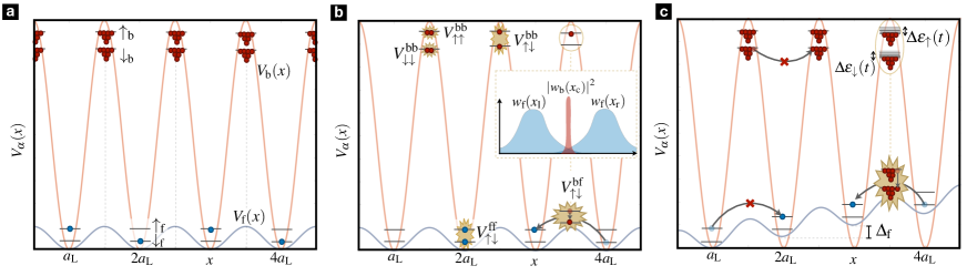
Figure 6: Cold-atom QS of the topological Schwinger model: (a) Bose-Fermi mixture trapped in a 1D optical lattice formed by a red-detuned very deep lattice for the bosons (red circles trapped in two internal states at the maxima), and a blue-detuned shallower lattice for the fermions (blue circles trapped in two internal states at the minima). (b) Dominant scattering processes, including on-site boson-boson and fermion-fermion Hubbard interactions, as well as boson-fermion spin-changing collisions allowed by the common overlap of neighboring Wannier functions for the fermions, weighted by the probability to find a boson on the intermediate link. (c) Inhibition of the bosonic and fermionic bare tunnelings, either due to the very deep bosonic lattice, or to the application of a lattice tilting for the fermions. The spin-changing collisions can be assisted against the lattice tilting introducing a periodic modulation of the bosonic energy levels.

IV Cold-atom quantum simulations of the topological Schwinger model

The remarkable level of isolation and control in several platforms of atomic, molecular and optical (AMO) physics, such as ultra-cold neutral atoms in periodic crystals made of light  QS_cold_atoms or trapped atomic ions in self-assembled Coulomb crystals QS_trapped_ions , has allowed to conduct experiments in the recent years bringing the quantum simulation (QS) idea feynman_qs to a practical reality. Starting with the pioneering works showing that ultra-cold bosonic atoms can be used for the QS of the Bose-Hubbard model analog_QS_bhm_exp , a variety of schemes for the QS of condensed-matter models have been put forth qs_book . In recent years, several works have explored the possibility of using AMO systems for the QS of relativistic fermionic and bosonic quantum field theories aqs_qft_fermions_2d ; aqs_qft_fermions ; aqs_qft_fermions_interactions ; dqs_qft_phi4 ; O_N_models ; aqs_phi_4 , theories of pure gauge fields dqs_lattice_gauge_theories ; aqs_qft_gauge_U(1)_qlinks ; aqs_qft_gauge_U(1)_qlinks2 ; dqs_qft_SU(2)_qlinks ; loops_and_strings_gauge_simulator , theories for coupled Higgs and gauge fields gauge_higgs_atoms ; gauge_higgs_meurice , and also theories of relativistic fermions interacting with Abelian and non-Abelian gauge fields aqs_QED ; aqs_qft_fermions_U(1)_qlinks ; aqs_qft_fermions_SU(2)_qlinks . Although most proposals have focused on ultracold atoms in optical lattices, we note that QS of gauge fields has also been explored for crystals of trapped ions, arrays of superconducting qubits and microwave resonators, and atom-ion mixtures gauge_other_systems .

Of particular relevance for our work will be the QS schemes for the simplest possible theory of matter coupled to gauge fields: quantum electrodynamics in (1+1) dimensions, or the so-called Schwinger model. We refer the reader to existing literature reviewing these schemes, and extensions thereof qs_LGT_review ; schwinger_mps_review , and to the recent experiments schwinger_experiments realizing a digital QS (and a variational eigensolver of the massive Schwinger model). We note that there has also been recent progress on the analog QS of dynamical gauge fields int_pat ; density_dep_gauge_fields ; z2_gauge_prop ; z2_gauge_exp . In the following, we will focus on analog QS of the topological Schwinger model (4) using a Bose-Fermi mixture of ultra-cold neutral atoms trapped in an optical lattice.

IV.1 Bose-Fermi mixtures for lattice gauge theories

We consider bosonic (fermionic) alkali atoms of mass $m_{\rm b}$ ($m_{\rm f}$), and select a pair of electronic states $\{\ket{\uparrow_{\alpha}}=\ket{F_{\alpha},M_{\alpha,\uparrow}},\ket{\downarrow_{\alpha}}=\ket{F_{\alpha},M_{\alpha,\downarrow}}\}_{\alpha={\rm b,f}}$ from the hyperfine ground-state manifold, which will be referred to as spin components $\sigma=\uparrow,\downarrow$. The atoms are trapped in a spin-independent cubic optical lattice formed by pairs of retro-reflected far-detuned laser beams with mutually-orthogonal linear polarizations, which lead to periodic ac-Stark shifts of strength $\{V_{0,j}^{\alpha}\}_{j=x,y,z}$ cold_atoms_ol . The common wavelength of the lasers $\lambda_{\rm L}=2\pi/k_{\rm L}$ sets the lattice constant of the periodic light potential to $a_{\rm L}=\lambda_{\rm L}/2$ along each of the three axes. We will assume that $V_{0,x}^{\alpha}\ll V_{0,y}^{\alpha},V_{0,z}^{\alpha}$, such that the dynamics along the $y$ and $z$ axes is effectively frozen, and the atomic mixture behaves as a 1D system along the $x$ axis.

We consider a regime with a lattice depth that is much larger than the atomic recoil energy $V_{0,x}^{\alpha}\gg E_{\rm R}^{\alpha}=k_{\rm L}^{2}/2m_{\alpha}$, where we work with $\hbar=1$ as usual in the cold-atom literature. In this regime, the atoms are confined to small regions around the minima/maxima of the optical potential, depending on the sign of the laser detuning. Therefore, it is customary to introduce the so-called Wannier basis  analog_QS_bhm ; analog_QS_fhm ; analog_QS_bfhm , and define operators that create/annihilate bosonic $b^{\dagger}_{n,\sigma},b^{\phantom{\dagger}}_{n,\sigma^{\prime}}$ and fermionic $f^{\dagger}_{n,\sigma},f^{\phantom{\dagger}}_{n,\sigma^{\prime}}$ atoms localized at such positions, satisfying $[b^{\phantom{\dagger}}_{n,\sigma},b^{\dagger}_{m,\sigma}]=\{f^{\phantom{\dagger}}_{n,\sigma},f^{\dagger}_{m,\sigma}\}=\delta_{n,m}\delta_{\sigma,\sigma^{\prime}}$. For a fermionic blue-detuned optical potential along the $x$ axis, the fermions would be trapped at the minima $x_{n}^{0}=na_{\rm L}$, where $n\in\mathbb{Z}_{N_{\rm s}}$ is the site index and $N_{\rm s}$ is the number of lattice sites; whereas the bosons are trapped at the maxima $x_{n}^{0}=(n+\textstyle\frac{1}{2})a_{\rm L}$ of a red-detuned optical potential (see Fig. 6(a)). In this way, one may interpret that fermions reside at the sites of a 1D chain and will be used to represent the matter sector of the topological Schwinger model, while bosons sit at the links and will be employed to simulate the gauge field.

The dynamics of the Bose-Fermi mixture is controlled by the following lattice Hamiltonian

$$\begin{split}H_{\rm BF}&=\sum_{n,\sigma}(\epsilon^{\rm b}_{n,\sigma}b^{\dagger}_{n,\sigma}b^{\phantom{\dagger}}_{n,\sigma}-t_{\rm b}b^{\dagger}_{n,\sigma}b^{\phantom{\dagger}}_{n+1,\sigma}+{\rm H.c.})+\\ &+\sum_{n,\sigma}(\epsilon^{\rm f}_{n,\sigma}f^{\dagger}_{n,\sigma}f^{\phantom{\dagger}}_{n,\sigma}-t_{\rm f\hskip 1.50694pt}f^{\dagger}_{n,\sigma}f^{\phantom{\dagger}}_{n+1,\sigma}\hskip 2.15277pt+{\rm H.c.})+V_{\rm int},\end{split}$$ (19)

where we have introduced on-site energy terms $\epsilon^{\alpha}_{n,\sigma}$ that will depend on the energy of the electronic states including e.g. hyperfine energy of the electronic states and an overall harmonic trapping potential. In this expression, we have introduced the tunneling strength $t_{\alpha}=4E_{\rm R}^{\alpha}({V}_{0,x}^{\alpha}/E_{\rm R}^{\alpha})^{3/4}{\rm exp}\{-2({V}_{0,x}^{\alpha}/E_{\rm R}^{\alpha})^{1/2}\}/\sqrt{\pi}$ cold_atoms_ol , which controls the hopping of fermionic/bosonic atoms between neighboring sites/links of the 1D chain. Additionally, at sufficiently low temperatures, the atoms interact via $s$-wave scattering through a contact pseudo-potential cold_atoms_ol . In the Wannier basis, this yields various quartic terms grouped in $V_{\rm int}$ as follows

$$\begin{split}V_{\rm int}=&\sum_{\bm{n},\bm{\sigma}}\textstyle\frac{1}{2}V^{\rm b,b}_{\bm{n},\bm{\sigma}}b^{\dagger}_{n_{1},\sigma_{1}}b^{\dagger}_{n_{2},\sigma_{2}}b^{\phantom{\dagger}}_{n_{4},\sigma_{4}}b^{\phantom{\dagger}}_{n_{3},\sigma_{3}}\\ +&\sum_{\bm{n},\bm{\sigma}}\textstyle\frac{1}{2}V^{\rm f,f}_{\bm{n},\bm{\sigma}}f^{\dagger}_{n_{1},\sigma_{1}}f^{\dagger}_{n_{2},\sigma_{2}}f^{\phantom{\dagger}}_{n_{4},\sigma_{4}}f^{\phantom{\dagger}}_{n_{3},\sigma_{3}}\\ +&\sum_{\bm{n},\bm{\sigma}}V^{\rm f,b}_{\bm{n},\bm{\sigma}}f^{\dagger}_{n_{1},\sigma_{1}}b^{\dagger}_{n_{2},\sigma_{2}}b^{\phantom{\dagger}}_{n_{4},\sigma_{4}}f^{\phantom{\dagger}}_{n_{3},\sigma_{3}}.\\ \end{split}$$ (20)

Here, $\bm{n}=(n_{1},n_{2},n_{3},n_{4})$ and $\bm{\sigma}=(\sigma_{1},\sigma_{2},\sigma_{3},\sigma_{4})$ determine the positions and spin (i.e. electronic) states of the colliding atoms $(n_{1},\sigma_{1})+(n_{2},\sigma_{2})\to(n_{3},\sigma_{3})+(n_{4},\sigma_{4})$, and $V^{\alpha_{1},\alpha_{2}}_{\hskip 1.50694pt\bm{n},\hskip 1.50694pt\bm{\sigma}}$ determines the strength of the corresponding scattering process, which involves a particular overlap of different Wannier functions. For deep optical lattices, these interaction strengths decay exponentially fast with the distance separating the corresponding Wannier centers, such that the leading contributions will be fermion-fermion (boson-boson) on-site (on-link) interactions, as well as boson-fermion interactions between site-link nearest neighbors (see Fig. 6(b)).

As realized in gauge_int_ang_mome_cons , it is possible to exploit the conservation of total angular momentum in the $s$-wave atomic scattering to identify those terms of Eq. (20) that incorporate directly the gauge invariance of a LGT, such as the $U(1)$ gauge invariance of the standard Schwinger model (3). In particular, with a suitable encoding, the boson-boson on-site interactions can give rise to the electric energy term $g^{2}L_{n}^{2}$. Additionally, the boson-fermion spin-changing scattering can lead to the gauge-invariant tunnelings $c_{n}^{\dagger}U^{\phantom{\dagger}}_{n}c_{n+1}^{\phantom{\dagger}}+c_{n+1}^{\dagger}U^{\dagger}_{n}c_{n}^{\phantom{\dagger}}$, where the link operators can be represented by spin ladder operators $U_{n}\to L_{n}^{+},U^{\dagger}_{n}\to L_{n}^{-}$ satisfying $[L^{+}_{n},L^{-}_{m}]=2\delta_{n,m}L_{n}$, following the so-called quantum-link model approach to LGTs q_link_models . A detailed analysis of how this idea could be applied to a ²³Na-⁶Li Bose-Fermi mixture has been presented in Schwinger_spin_changing_collisions_superlattice , where the fermions were considered to be trapped in an optical superlattice providing a staggering of the on-site energies. This work showed that, in addition to the above mechanism to generate the gauge-invariant tunneling, the terms of Eqs. (19) and (20) that would violate gauge invariance can be neglected for certain parameter regimes and initial states, as will be discussed below. Moreover, it was shown that the additional spin-preserving scattering between bosons and fermions can be expressed as a correction of the staggered fermion mass of the target Hamiltonian (3). In this way, there is a clear route for the analog quantum simulation of the standard Schwinger model. Although challenging, we note that the individual required ingredients have all been shown experimentally, e.g. the types of optical lattices required, experiments with two-species Bose-Fermi mixtures, the control of Feshbach resonances, etc. The future technological quest is their combination in a single experiment in the particular suitable regime for a LGT simulator.

IV.2 Scheme for the topological Schwinger model

Let us now turn our attention to the cold-atom quantum simulation of the topological Schwinger model (4). Here, a natural idea would be to substitute the aforementioned staggered fermion superlattice by a superlattice where the distance between neighboring fermions varies within a two-site unit cell. Such optical potentials have already been realized experimentally, and yield a dimerized tunneling that allows for the cold-atom quantum simulation ssh_cold_atoms of the SSH model of polyacetylene. One can check that this mechanism would also lead to a dimerization of the gauge-invariant tunneling (4), since the fermion-boson overlap of Wannier functions determining the strength of the spin-changing collisions would also display a two-site unit cell periodicity. Unfortunately, the spin-conserving scattering terms also become inhomogeneous, and can no longer be simplified as in the previous case Schwinger_spin_changing_collisions_superlattice , such that the effective cold-atom Hamiltonian would contain additional terms that differ from the target model (4). Therefore, in this work, we introduce a scheme that avoids using superlattices, and achieves the desired dimerization by Floquet engineering through a periodic modulation on the bosonic degrees of freedom. We now detail the required ingredients.

IV.2.1 Gauge sector and bosonic Hubbard interactions

Let us start from the bosons and the gauge-field sector. First of all, we consider that the bosonic optical lattice is so deep $V_{0,x}^{\rm b}\gg E_{\rm R}^{\rm b}$ that the tunneling dynamics along the $x$-axis is also frozen for the time-scales of interest $t_{\rm b}\propto E_{\rm R}^{\rm b}{\rm exp}\{-2({V}_{0,x}^{\alpha}/E_{\rm R}^{\rm b})^{1/2}\}\ll|V^{\alpha,\beta}_{\bm{n},\bm{\sigma}}|$. Using the Schwinger representation for spin operators in terms of bosons, referred to as rishons in the quantum link models, one can encode the link gauge operators on even sites into the bosonic atoms as

$$\begin{split}L_{2n}&=\frac{1}{2}\left(b^{\dagger}_{2n,\uparrow}b^{\phantom{\dagger}}_{2n,\uparrow}-b^{\dagger}_{2n,\downarrow}b^{\phantom{\dagger}}_{2n,\downarrow}\right),\\ L_{2n}^{+}&=b^{\dagger}_{2n,\uparrow}b^{\phantom{\dagger}}_{2n,\downarrow},\hskip 8.61108ptL_{2n}^{-}=b^{\dagger}_{2n,\downarrow}b^{\phantom{\dagger}}_{2n,\uparrow},\end{split}$$ (21)

and the link gauge operators on odd sites as

$$\begin{split}L_{2n-1}&=\frac{1}{2}\left(b^{\dagger}_{2n-1,\downarrow}b^{\phantom{\dagger}}_{2n-1,\downarrow}-b^{\dagger}_{2n-1,\uparrow}b^{\phantom{\dagger}}_{2n-1,\uparrow}\right),\\ L_{2n-1}^{+}&=b^{\dagger}_{2n-1,\downarrow}b^{\phantom{\dagger}}_{2n-1,\uparrow},\hskip 8.61108ptL_{2n-1}^{-}=b^{\dagger}_{2n-1,\uparrow}b^{\phantom{\dagger}}_{2n-1,\downarrow}.\end{split}$$ (22)

We note that the seemingly-arbitrary alternation in the definition of the link operators is important to obtain the gauge-invariant tunneling from the spin-changing collisions gauge_int_ang_mome_cons ; Schwinger_spin_changing_collisions_superlattice . We also note that, since the bare bosonic tunneling can be neglected, the number of bosons with a particular spin $\sigma$ is a conserved quantity, and can be used to define the angular momentum of the link operators $\ell=N_{\uparrow}=N_{\downarrow}$ where, for simplicity, we assume that all sites are uniformly filled with bosons, and that the population is the same for both spin components.

As announced above, the on-site boson-boson interactions of Eq. (20) can be expressed in terms of the electric-flux energy of the Schwinger model. For a ²³Na-⁶Li Bose-Fermi mixture, and selecting the spin states $\ket{\uparrow_{\rm b}}=\ket{F_{\rm b}=1,M_{\rm b,\uparrow}=0},\ket{\downarrow_{\rm b}}=\ket{F_{\rm b}=1,M_{\rm b,\downarrow}=-1}$ Schwinger_spin_changing_collisions_superlattice , the on-site Hubbard-type interactions can be expressed as follows

$$V_{\rm int}^{\rm bb}=a\sum_{n=0}^{N_{\rm s}-1}\left(\delta_{\rm b}(-1)^{n}L_{n}+\frac{1}{2}g^{2}L_{n}^{2}\right).$$ (23)

Here, we have introduced an effective gauge coupling $g$ and an effective lattice constant $a$, which can be expressed in terms of the atomic parameters

$$g^{2}a=2\sqrt{\frac{8}{\pi}}k_{\rm L}\left(\frac{a^{\rm bb}_{0}-a^{\rm bb}_{2}}{6}\right)E_{\rm R}^{\rm b}\left(\frac{V_{0,x}^{\rm b}V_{0,y}^{\rm b}V_{0,z}^{\rm b}}{(E_{\rm R}^{\rm b})^{3}}\right)^{1/4}.$$ (24)

Here, $a_{F_{\rm t}}^{\alpha\beta}$ stands for the $s$-wave scattering length between $\alpha$- and $\beta$-type atoms with total angular momentum $F_{\rm t}$. We note that, in addition to the desired electric-field energy, one gets in Eq. (23) an additional staggering $\delta_{\rm b}=(\ell-\textstyle\frac{1}{2})g^{2}$ that must be carefully accounted for in the final effective Hamiltonian of the cold-atom mixture.

IV.2.2 Matter sector and fermionic Hubbard interactions

Let us now turn to the matter sector of the topological Schwinger model (4), which should be encoded into the fermionic atoms. As occurred for the bosons, the bare tunneling (19) must be inhibited as it does not preserve the gauge symmetry. However, in contrast to the bosonic case, we cannot simply consider a very deep lattice, since neighboring fermionic Wannier functions should overlap to allow for the desired gauge-invariant tunneling via the spin-changing collisions. A possible mechanism to inhibit the bare tunneling could be a staggered superlattice Schwinger_spin_changing_collisions_superlattice , but we have already advanced that this would not suffice to achieve the desired topological Schwinger model (4). Therefore, we shall make use of a tilted optical lattice $\epsilon_{n,\sigma}^{\rm f}=\epsilon_{\sigma}^{\rm f}+\Delta_{\rm f}n$, which can be introduced by lattice acceleration lattice_acceleration , or magnetic-field gradients b_field_gradient . As a consequence of the tilting (see Fig. 6(c)), there is an energy penalty for the bare tunneling, such that fermions cannot hop between neighboring sites for the timescale of interest if $t_{\rm f}\ll\Delta_{\rm f}$, and the dynamics will be caused by scattering.

For the particular ²³Na-⁶Li Bose-Fermi mixture, and selecting the spin states $\ket{\uparrow_{\rm f}}=\ket{F_{\rm f}=\textstyle\frac{1}{2},M_{\rm f,\uparrow}=\textstyle\frac{1}{2}},\ket{\downarrow_{\rm f}}=\ket{F_{\rm f}=\textstyle\frac{1}{2},M_{\rm f,\downarrow}=-\textstyle\frac{1}{2}}$, one can encode the discretized Dirac field into the fermion atomic operators of even and odd sites

$$c_{2n}=\frac{1}{\sqrt{a}}f_{2n,\downarrow},\hskip 8.61108ptc_{2n-1}=\frac{1}{\sqrt{a}}f_{2n-1,\uparrow},$$ (25)

and recover the desired algebra $\{c_{n}^{\phantom{\dagger}},c_{m}^{\dagger}\}=\delta_{n,m}/a\to\delta(x-y)$ in the continuum limit. Moreover, the on-site fermion-fermion interactions of Eq. (20), which give the leading contribution of the fermion-fermion scattering, can be rewritten as

$$V_{\rm int}^{\rm ff}=a\sum_{n=0}^{N_{\rm s}-1}U\left(c^{\dagger}_{2n}c^{\phantom{\dagger}}_{2n}f^{\dagger}_{2n,\uparrow}f^{\phantom{\dagger}}_{2n,\uparrow}+c^{\dagger}_{2n-1}c^{\phantom{\dagger}}_{2n-1}f^{\dagger}_{2n-1,\downarrow}f^{\phantom{\dagger}}_{2n-1,\downarrow}\right),$$ (26)

where we have introduced the Hubbard coupling strength

$$Ua=\sqrt{\frac{8}{\pi}}k_{\rm L}a^{\rm ff}_{0}E_{\rm R}^{\rm f}\left(\frac{V_{0,x}^{\rm f}V_{0,y}^{\rm f}V_{0,z}^{\rm f}}{(E_{\rm R}^{\rm f})^{3}}\right)^{1/4}.$$ (27)

It follows from the above expression (26) that these interactions will have no effect if the state of the quantum simulator fulfills $f^{\dagger}_{2n,\uparrow}f^{\phantom{\dagger}}_{2n,\uparrow}\ket{\Psi(t)}=f^{\dagger}_{2n-1,\downarrow}f^{\phantom{\dagger}}_{2n-1,\downarrow}\ket{\Psi(t)}=0$ during the whole experiment. Since the bare tunneling is forbidden, and the lattice tilting forbids scattering terms that change the parity of fermions on each lattice site, it suffices to prepare an initial state $\ket{\Psi(0)}$ with no double occupancies (see the initial configuration in Fig. 6(a)), and the above condition to neglect these terms (26) will be fulfilled during the whole QS.

IV.2.3 Gauge-matter coupling and Floquet engineering of Bose-Fermi Hubbard interactions

Up to this point, the discussion is similar to the scheme in Schwinger_spin_changing_collisions_superlattice . In the following, we discuss the implementation of the dimerized gauge-invariant tunneling (4), where crucial differences arise. We now consider the fermion-boson site-link interactions (20), which contain the spin-changing collisions

$$\begin{split}V_{\rm int,1}^{\rm bf}&=\sum_{n=0}^{N_{\rm s}/2}V^{\rm f,b}_{\bm{n},\bm{\sigma}}f^{\dagger}_{2n-1,\uparrow}b^{\dagger}_{2n-1,\downarrow}b^{\phantom{\dagger}}_{2n-1,\uparrow}f^{\phantom{\dagger}}_{2n,\downarrow}\\ &+\sum_{n=0}^{N_{\rm s}/2}V^{\rm f,b}_{\bm{n},\bm{\sigma}}f^{\dagger}_{2n,\downarrow}b^{\dagger}_{2n,\uparrow}b^{\phantom{\dagger}}_{2n,\downarrow}f^{\phantom{\dagger}}_{2n+1,\uparrow}+{\rm H.c.}.\end{split}$$ (28)

These terms can be identified with the gauge-invariant tunneling $c_{n}^{\dagger}L^{+}_{n}c_{n+1}^{\phantom{\dagger}}+c_{n+1}^{\dagger}L^{-}_{n}c_{n}^{\phantom{\dagger}}$ using the atomic definitions of the link (21)-(22) and fermion operators (25). Note, however, that these terms will generally be inhibited by the tilting of the lattice $|V^{\rm f,b}_{\bm{n},\bm{\sigma}}|\ll\Delta_{\rm f}$, as occurred for the bare tunneling $t_{\rm f}\ll\Delta_{\rm f}$.

The key idea of our proposed scheme is to assist these terms by introducing a time-periodic modulation of the bosonic on-site energies $\epsilon_{n,\sigma}^{\rm b}\to\epsilon_{n,\sigma}^{\rm b}(t)$ of Eq. (19), which can be induced by a time-dependent magnetic field or by a weak ac-Stark shift with a time-dependent laser intensity (see Fig. 6(c)). In addition, we will adjust the static part $\epsilon_{\sigma}^{\alpha}$ of the fermionic and bosonic on-site energies through an external constant magnetic field. Altogether, we are considering the on-site energies

$$\epsilon_{n,\sigma}^{\rm b}(t)=\epsilon_{\sigma}^{\rm b}+\Delta^{\rm b}_{\sigma}\cos(\omega_{\rm d}t),\hskip 8.61108pt\epsilon_{n,\sigma}^{\rm f}=\epsilon_{\sigma}^{\rm f}+\Delta_{\rm f}n,$$ (29)

where $\epsilon_{\sigma}^{\alpha}=\epsilon_{F_{\alpha}}-g^{\rm L}_{F_{\alpha}}\mu_{\rm B}B_{0}M_{\alpha,\sigma}$ contains the hyperfine electronic energy $\epsilon_{F_{\alpha}}$, and the contribution from the linear Zeeman shift, where $g^{\rm L}_{F_{\alpha}}$ is the so-called Lande factor, $\mu_{\rm B}$ is Bohr’s magneton, and $B_{0}$ the external constant magnetic field. In the simplest situation, the periodic modulation stems from an ac-Stark shift $\Delta^{\rm b}_{\sigma}=-\alpha_{\sigma}(\omega_{\rm L})I_{\rm L}$, where $\alpha_{\sigma}(\omega_{\rm L})$ is the spin-dependent dynamical polarizability of the state $\ket{F_{\alpha},M_{\alpha,\sigma}}$ irradiated by a far detuned laser beam of frequency $\omega_{\rm L}$ and intensity $I(t)=I_{\rm L}\cos(\omega_{\rm d}t)$, where $\omega_{\rm d}$ is the modulation frequency.

We consider adjusting the lattice tilting, external magnetic fields, and modulation frequency, such that

$$(\epsilon_{\uparrow}^{\rm b}-\epsilon_{\downarrow}^{\rm b})-(\epsilon_{\uparrow}^{\rm f}-\epsilon_{\downarrow}^{\rm f})=\Delta_{\rm f}+{\delta}_{\rm f},\hskip 12.91663pt\omega_{\rm d}=2\Delta_{\rm f},$$ (30)

where we have introduced a small energy mismatch $|\delta_{\rm f}|\ll\Delta_{\rm f}$. By writing the spin-changing scattering in Eq. (28) in the interaction picture with respect to these on-site energy terms, one finds

$$\begin{split}V_{\rm int,1}^{\rm bf}(t)&=a\sum_{n=0}^{N_{\rm s}/2}V^{\rm f,b}_{\bm{n},\bm{\sigma}}c^{\dagger}_{2n-1}L^{+}_{2n-1}c^{\phantom{\dagger}}_{2n}{\rm e}^{-{\rm i}t({\delta}_{\rm f}+2\Delta_{\rm f})}F(t)\\ &+a\sum_{n=0}^{N_{\rm s}/2}V^{\rm f,b}_{\bm{n},\bm{\sigma}}c^{\dagger}_{2n}L^{+}_{2n}c^{\phantom{\dagger}}_{2n+1}{\rm e}^{+{\rm i}t{\delta}_{\rm f}}F^{*}(t)+{\rm H.c.},\end{split}$$ (31)

where we have introduced the periodic function $F(t)={\rm exp}\{{\rm i}\eta_{\rm d}\sin(\omega_{\rm d}t)\}=\sum_{m\in\mathbb{Z}}J_{m}(\eta_{\rm d}){\rm e}^{{\rm i}m\omega_{\rm d}t}$, which is expressed in terms of Bessel functions of the first kind $J_{m}(\eta_{\rm d})$ with

$$\eta_{\rm d}=(\Delta^{\rm b}_{\downarrow}-\Delta^{\rm b}_{\uparrow})/\omega_{\rm d}.$$ (32)

Since we are working in the regime $|V^{\rm f,b}_{\bm{n},\bm{\sigma}}|\ll\Delta_{\rm f}$, and $\omega_{\rm d}=2\Delta_{\rm f}$, the rapidly-oscillating terms in the above expression (31) can be neglected in a rotating-wave approximation. This is equivalent to the large-frequency limit of the so-called Floquet engineering based on periodic modulations floquet_cold_atoms .

Moving back to a frame where the Hamiltonian is time-independent, we obtain the desired dimerized gauge-invariant tunneling

$$V_{\rm int,1}^{\rm bf}=a\sum_{n}\left(m_{\rm s}(-1)^{n}c_{n}^{{\dagger}}c_{n}^{\phantom{\dagger}}+\left(\frac{1}{a}(1-\delta_{n})c_{n}^{{\dagger}}L_{n}^{+}c_{n+1}^{\phantom{\dagger}}+{\rm H.c.}\right)\right),$$ (33)

where we have introduced an additional staggered mass $m_{\rm s}$, and the tunneling dimerization ${\delta}_{2n}=0$, and ${\delta}_{2n-1}=\Delta$, with

$$m_{\rm s}=\delta_{\rm f},\hskip 8.61108pt\Delta=1-\frac{J_{1}(\eta_{\rm d})}{J_{0}(\eta_{\rm d})}.$$ (34)

Finally, the effective lattice constant of the topological Schwinger model (4) is set by the overlap of the neighboring Wannier functions

$$\frac{1}{a}={\frac{k_{\rm L}\bigg{(}a^{\rm bf}_{\frac{3}{2}}-a^{\rm bf}_{\frac{1}{2}}\bigg{)}}{3\sqrt{2\pi}}}E_{\rm R}^{\rm f}\!\left(\!\!\frac{V_{0,x}^{\rm f}V_{0,x}^{\rm f}V_{0,x}^{\rm f}}{(E_{\rm R}^{\rm f})^{3}}\!\!\right)^{\!\!\textstyle\frac{1}{4}}\!\!\frac{m_{\rm f}}{\mu_{\rm bf}}{\rm e}^{-\frac{\pi^{2}}{8}\sqrt{\frac{V_{0,x}^{\rm f}}{E_{\rm R}^{\rm f}}}}J_{0}(\eta_{\rm d}),$$ (35)

where we have used the reduced mass $\mu_{\rm bf}=m_{\rm b}m_{\rm f}/(m_{\rm b}+m_{\rm f})$, and assumed that the bosons are subjected to a much tighter confinement than the fermions.

It thus follows from our analysis that the effective dimerization $\Delta$ in the target model (4) can be controlled by tuning the periodic-modulation parameters in Eq. (32). Likewise, the dimensionless gauge coupling $ga$ can be controlled by tuning the trapping and modulation parameters, as well as the various scattering lengths appearing in Eqs. (24) and (35). In this way, one could explore the full phase diagram of the topological Schwinger model provided that the additional staggered terms in Eqs. (23) and (33) are carefully accounted for. We also note that the cold-atom simulator does not work in natural units, but leads instead to an effective speed of light $c=a_{\rm L}/a$. In any case, the fields have the correct energy dimensions $d_{c}=1/2$ and $d_{L}=0$, while the mass and gauge coupling have $d_{m_{s}}=d_{g}=1$, and the effective lattice constant $d_{a}=-1$.

IV.2.4 Suppression of additional spurious terms

Let us note that, in addition to the terms leading to Eq. (33), there are other density-dependent tunneling terms inhibited in principle by the tilting, which would also get activated by the periodic modulation. However, these terms can be neglected using the same argument used below Eq. (27). In addition, there will be additional spin-conserving scattering terms that are not inhibited by the lattice tilting that require a more careful account. These terms can be expressed as

$$\begin{split}V_{\rm int,2}^{\rm bf}&=a\sum_{n,\sigma_{2}}V^{\rm f,b}_{\bm{n},\bm{\sigma}}c^{\dagger}_{2n}c^{\phantom{\dagger}}_{2n}(b^{\dagger}_{2n-1,\sigma_{2}}b^{\phantom{\dagger}}_{2n-1,\sigma_{2}}+b^{\dagger}_{2n,\sigma_{2}}b^{\phantom{\dagger}}_{2n,\sigma_{2}})\\ &+a\sum_{n,\sigma_{2}}V^{\rm f,b}_{\bm{n},\bm{\sigma}}c^{\dagger}_{2n+1}c^{\phantom{\dagger}}_{2n+1}(b^{\dagger}_{2n,\sigma_{2}}b^{\phantom{\dagger}}_{2n,\sigma_{2}}+b^{\dagger}_{2n+1,\sigma_{2}}b^{\phantom{\dagger}}_{2n+1,\sigma_{2}}).\end{split}$$ (36)

The fact that the fermionic density $c^{\dagger}_{n}c^{\phantom{\dagger}}_{n}$ is coupled equally to the rightmost and leftmost neighboring bosons, which underlies the form of Eq. (36), allows us to express this scattering in terms of the finite gradient of the flux operators $(L_{n}-L_{n-1})$ via Eqs. (21)-(22). We note that this is precisely the condition that would not be satisfied had we used an optical superlattice, and which forced us to consider a Floquet-type alternative to achieve the tunneling dimerization.

This expression (36) can in turn be simplified further by applying Gauss’ law $({L}_{n}-{L}_{n-1})=ac_{n}^{\dagger}c_{n}+\textstyle\frac{1}{2}((-1)^{n}-1)$ for the particular sector of the initial state of the cold-atom quantum simulator Schwinger_spin_changing_collisions_superlattice . This allows us to rewrite the spin-conserving scattering as a correction to the fermion staggered mass

$$V_{\rm int,2}^{\rm bf}=a\sum_{n}\tilde{m}_{\rm s}(-1)^{n}c_{n}^{\dagger}c_{n}^{\phantom{\dagger}},$$ (37)

up to an irrelevant constant term, where we have introduced

$$\tilde{m}_{\rm s}={\frac{k_{\rm L}\bigg{(}a^{\rm bf}_{\frac{3}{2}}-a^{\rm bf}_{\frac{1}{2}}\bigg{)}}{\sqrt{\pi/2}}}\frac{\ell-2}{6}E_{\rm R}^{\rm f}\!\left(\!\!\frac{V_{0,x}^{\rm f}V_{0,x}^{\rm f}V_{0,x}^{\rm f}}{(E_{\rm R}^{\rm f})^{3}}\!\!\right)^{\!\!\textstyle\frac{1}{4}}\!\!\frac{m_{\rm f}}{\mu_{\rm bf}}{\rm e}^{-\frac{\pi^{2}}{4}\sqrt{\frac{V_{0,x}^{\rm f}}{E_{\rm R}^{\rm f}}}}.$$ (38)

As announced previously, the additional staggering terms must be carefully accounted for, as they do not appear in the target topological Schwinger model (4). In our case, their effect can be cancelled by controlling the detuning of the periodic modulation (30). It is straightforward to see that in the interaction picture with respect to $H_{0}=a\sum_{n}\left(\delta_{\rm b}(-1)^{n}L_{n}+(m_{\rm s}+\tilde{m}_{\rm s})c_{n}^{\dagger}c_{n}^{\phantom{\dagger}}\right)$, the cold-atom Hamiltonian $H=V_{\rm int}^{\rm bb}+V_{\rm int,1}^{\rm bf}+V_{\rm int,2}^{\rm bf}=H_{0}+H_{t{\rm S}}$, leads to an effective time-independent Hamiltonian that coincides exactly with the topological Schwinger model $H_{\rm eff}=H_{t{\rm S}}$ (4), provided that

$$\delta_{\rm f}=\textstyle\frac{1}{2}\delta_{\rm b}-\tilde{m}_{\rm s}.$$ (39)

Accordingly, by tuning the energy mismatch between the energy-penalty and the modulation frequency (30), it is possible to reach a situation where the staggered mass effectively vanishes from the Hamiltonian and, as desired, the Schwinger model only displays a topological mass stemming from the tunneling dimerization.

Let us finally note that, for simplicity of exposition, we have assumed that the atoms are subjected to a box trapping potential box_potential_cold_atoms , and thus neglected additional inhomogeneities of the on-site energies (29). For other trapping potentials, it suffices to assume that they vary slowly on the length-scale of the optical-lattice spacing, such that their presence will not compromise our assumptions and calculations above, and can be simply included as some additional inhomogeneities in the final effective Hamiltonian $H_{t{\rm S}}$. Alternatively, one could also decide to explore the more general phase diagram $(\Delta,m_{\rm s}a,ga)$, where the staggered mass $m_{\rm s}$ introduces another microscopic mechanism that competes with the dimerized topological mass $\Delta/a$, and will eventually lead to a trivial band insulator instead of the the SPT phase. In the future, it would be interesting to study the phase diagram of this model using the analytical and numerical techniques discussed in this work. We advance that, although the staggered mass will break the global symmetries table_ti that protect the SPT phase spt_schwinger , there will always be a local inversion symmetry, such that the SPT phase becomes a topological crystalline insulator review_classification .

IV.2.5 State preparation and readout

Since the model parameters $(ga,\Delta)$ are controlled by atomic parameters in Eqs. (24), (35) and (32), the cold-atom quantum simulator has the potential of realizing the interesting physics of topological QED₂ outlined in previous sections. In particular, by adiabatic state preparation, the cold-atom mixture could explore the full phase diagram of Fig. 1, provided that some of the observables discussed in Sec. III can be measured experimentally. Density-type observables, such as the electric-field order parameter (12), which is expressed in terms of the atomic densities (21)-(22), are particularly promising as they are not modified by the various interaction pictures and rotating frames discussed above. We note that the required spin-resolved density measurements can be performed by optical imaging, either after a time-of-flight expansion or directly in situ ketterle_reviews . On the other hand, the topological correlator (14) will be modified by the tilting and effective staggering in the final rotating frame. In this case, it would be interesting to explore if spin-resolved local measurements by using recent quantum gas microscopes microscopes can give access to the local quantities, such that the corresponding rotating-frame order parameter can be constructed from a specific combination of the different local measurements.

An alternative readout possibility would be to measure directly the edge excitations edge_excitations_measurement , which should display the dependence discussed in Ref. spt_schwinger . Although the above calculation uses Dirichlet boundary conditions, and would thus require the use of box-like trapping potentials box_potential_cold_atoms , a similar behavior is expected for confining potentials that increase at least quadratically with the boundary-to-center distance edge_detection . In that work, the authors also discuss how to use the Bragg signal due to Raman excitations to detect the presence of localized zero-energy modes in a higher-dimensional setup, and these ideas could be adapted to the current topological Schwinger model (4).

Finally, let us mention another readout strategy, which rests upon the possibility of measuring directly the underlying topological invariant. In the non-interacting regime, we note that the Zak’s phase zak_phase ; berry_rmp has already been measured using Ramsey interferometry in cold-atom experiments ssh_cold_atoms . As the gauge coupling is switched on, one expects that the fermionic excitations will become quasiparticles, which can be coupled to additional impurities in order to generalize the interferometric protocol to measure a many-body counterpart of the topological Zak’s phase many_body_zak .

V Conclusions and outlook

In this work, we have explored the interplay of global and local symmetries, topology, and many-body effects in symmetry-protected topological phases of matter that arise naturally in lattice gauge theories. We have presented a detailed study of the topological Schwinger model by means of a class of $\mathbb{Z}_{N}$ lattice gauge theories showing that these models host a correlated topological phase for different values of $N$, where interactions are mediated by the gauge field. By a careful finite-size scaling, we have shown that this phase is stable in the large-$N$ limit, and that the phase boundaries are in accordance to bosonization predictions of the $U(1)$ topological Schwinger model. Finally, we have presented a detailed proposal for the realization of the topological Schwinger model exploiting spin-changing collisions in boson-fermion mixtures of ultra-cold atoms loaded in a 1D optical lattice. We have shown that, by introducing a lattice tilting on the fermions and a periodic modulation of the bosons, the effective Hamiltonian coincides with the target topological Schwinger model with parameters that can be controlled by tuning the microscopic cold-atom parameters. In combination with the recent work spt_gauge , which studies the appearance of SPT phase in quantum link ladders, our work opens an interesting route to study topological phases of matter in gauge theories, either using some of the theoretical tools hereby developed, or via cold-atom experiments using the scheme proposed in this work. Hopefully, these results will stimulate further work in this subject, exploring interesting questions such as the interplay of topological features with non-perturbative effects in LGTs, such as screening, confinement, and string-breaking. In addition, it will be very interesting to explore the appearance of topological properties in a non-equilibrium situation where the quantum-mechanical $\hat{\theta}$ angle is quenched. For a sudden quench in the classical vacuum $\theta$ angle, very interesting dynamical topological phase transitions have been identified in dynamical_topo_transition_theta_angle by exploring bulk phenomena. Our approach would allow to have an edge perspective of these phenomena, and explore the consequences of a quantum-mechanical $\hat{\theta}$ angle.

- (1) L. Landau, Theory of phase transformations Zh. Eksp. Teor. Fiz. 7, 19 (1937) [Phys. Z. Sowjetunion 11, 26 (1937)]
- (2) K. V. Klitzing, G. Dorda, and M. Pepper, New Method for High-Accuracy Determination of the Fine-Structure Constant Based on Quantized Hall Resistance, Phys. Rev. Lett. 45, 494 (1980).
- (3) D. J. Thouless, M. Kohmoto, M. P. Nightingale, and M. den Nijs, Quantized Hall Conductance in a Two-Dimensional Periodic Potential Phys. Rev. Lett. 49, 405 (1982).
- (4) F. D. M. Haldane, Model for a Quantum Hall Effect without Landau Levels: Condensed-Matter Realization of the Parity Anomaly, Phys. Rev. Lett. 61, 2015 (1988).
- (5) C. L. Kane and E. J. Mele, Z2 Topological Order and the Quantum Spin Hall Effect, Phys. Rev. Lett. 95, 146802 (2005).
- (6) M. Z. Hasan and C. L. Kane, Colloquium: Topological insulators, Rev. Mod. Phys. 82, 3045 (2010).
- (7) X.-L. Qi and S.-C. Zhang, Topological insulators and superconductors, Rev. Mod. Phys. 83, 1057 (2011).
- (8) A. Bansil A, H. Lin, and T. Das, Colloquium: Topological band theory, Rev. Mod. Phys. 88, 021004 (2016).
- (9) D. C. Tsui, H. L. Stormer, and A. C. Gossard, Two-Dimensional Magnetotransport in the Extreme Quantum Limit, Phys. Rev. Lett. 48, 1559 (1982).
- (10) R. B. Laughlin, Anomalous Quantum Hall Effect: An Incompressible Quantum Fluid with Fractionally Charged Excitations Phys. Rev. Lett. 50, 1395 (1983).
- (11) M. Hohenadler, and F. F. Assaad, Correlation effects in two-dimensional topological insulators, J. Phys.: Condens. Matter 25, 143201 (2013); S.A. Parameswaran, R. Roy, and S.L. Sondhi,Fractional quantum Hall physics in topological flat bands, Compt. Rend. Phys. 14, 816 (2013).
- (12) L. Cardarelli, S. Greschner, and L. Santos, Hidden Order and Symmetry Protected Topological States in Quantum Link Ladders, Phys. Rev. Lett. 119, 180402 (2017).
- (13) G. Magnifico, D. Vodola, E. Ercolessi, S. P. Kumar, M. M ller, and A. Bermudez, Symmetry-protected topological phases in lattice gauge theories: topological QED2, Phys. Rev. D 99, 014503 (2019).
- (14) D. González-Cuadra, A. Dauphin, P. R. Grzybowski, P. Wójcik, M. Lewenstein, and A. Bermudez, Symmetry-Breaking Topological Insulators in the Bose-Hubbard Model, Phys. Rev. B 99, 045139 (2019).
- (15) D. González-Cuadra, A. Bermudez, P. R. Grzybowski, M. Lewenstein, and A. Dauphin, Intertwined Topological Phases induced by Emergent Symmetry Protection, arXiv:1903.01911 (2019).
- (16) C. N. Yang and R. L. Mills, Conservation of isotopic spin and isotopic gauge invariance, Phys. Rev. 96, 191 (1954).
- (17) M. E. Peskin, and D. V. Schröder, An Introduction to Quantum Field Theory (Addison-Wesley, Reading, 1995).
- (18) K. G. Wilson, Phys. Rev. D 10, 2445 (1974).
- (19) C. Gattringer, and C. B. Lang, Quantum Chromodynamics on the Lattice: An Introductory Presentation, Lect. Notes Phys. 788 (Springer, Berlin Heidelberg 2010).
- (20) J. B. Kogut, An introduction to lattice gauge theory and spin systems, Rev. Mod. Phys. 51, 659 (1979).
- (21) D. B. Kaplan, A method for simulating chiral fermions on the lattice, Phys. Lett. B 288, 342 (1992).
- (22) D. B. Kaplan, Chiral Symmetry and Lattice Fermions, arXiv:0912.2560 (2009).
- (23) K. Jansen and M. Schmaltz, Phys. Lett. B 296, 374 (1992); K. Jansen, Chiral fermions and anomalies on a finite lattice Phys. Lett. B 288, 348 (1992); Y. Shamir, Chiral fermions from lattice boundaries, Nuc. Phys. B 406, 90 (1993); M. F. Golterman, K. Jansen, and D. B. Kaplan, Chern-Simons currents and chiral fermions on the lattice, Phys. Lett. B 301, 219 (1993).
- (24) J. Schwinger, Gauge Invariance and Mass. II, Phys. Rev. 128, 2425 (1962).
- (25) L. S. Brown, Nuovo Cimento 29, 617 (1963).
- (26) J. Kogut and L. Susskind, Phys. Rev. D 11, 3594 (1975).
- (27) J. Kogut and L. Susskind, Hamiltonian formulation of Wilson’s lattice gauge theories, Phys. Rev. D 11, 395 (1975).
- (28) S. Coleman, R. Jackiw, and L. Susskind, Charge shielding and quark confinement in the massive schwinger model, Ann. Phys. 93, 267 (1975).
- (29) S. Coleman, More about the massive Schwinger model, Ann. Phys. 101, 239 (1976).
- (30) X.-L. Qi, T. L. Hughes, and S.-C. Zhang, Topological field theory of time-reversal invariant insulators, Phys. Rev. B 78, 195424 (2008); X.-L. Qi, R. Li, J. Zang, and S.-C. Zhang, Inducing a magnetic monopole with topological surface states, Science 323, 1184 (2009).
- (31) D. Horn, M. Weinstein, and S. Yankielowicz, Hamiltonian approach to Z(N) lattice gauge theories, Phys. Rev. D 19, 3715 (1979).
- (32) S. Notarnicola, E. Ercolessi, P. Facchi, G. Marmo, S. Pascazio and F. V. Pepe, Discrete Abelian Gauge Theories for Quantum Simulations of QED, J. Phys. A: Math. Theor. 48, 30FT01 (2015).
- (33) S. Kühn, J. I. Cirac, and M.-C. Bañuls, Quantum simulation of the Schwinger model: A study of feasibility, Phys. Rev. A 90, 042305 (2014).
- (34) E. Ercolessi, P. Facchi, G. Magnifico, S. Pascazio, F. V. Pepe, Phase Transitions in Zn Gauge Models: Towards Quantum Simulations of the Schwinger-Weyl QED, Phys. Rev. D 98, 074503 (2018).
- (35) I. Bloch, J. Dalibard, and S. Nascimbene, Quantum simulations with ultracold quantum gases, Nat. Phys. 8, 267 (2012).
- (36) R. Blatt and C. F. Roos, Quantum simulations with trapped ions, Nat. Phys. 8, 277 (2012).
- (37) R. P. Feynman, Simulating physics with computers, Int. J. Theor. Phys. 21, 467 (1982).
- (38) J. I. Cirac and P. Zoller, Goals and opportunities in quantum simulation, Nat. Phys. 8, 264 (2012).
- (39) U.-J. Wiese, Ultracold Quantum Gases and Lattice Systems: Quantum Simulation of Lattice Gauge Theories, Ann. Phys. 525, 777 (2013); E. Zohar, J. I. Cirac, and B. Reznik, Quantum simulations of lattice gauge theories using ultracold atoms in optical lattices, Rep. Prog. Phys. 79, 014401 (2015).
- (40) A. Eckardt, Colloquium: Atomic quantum gases in periodically driven optical lattices, Rev. Mod. Phys. 89, 011004 (2017).
- (41) R. S. Knox, Theory of Excitons (Solid state physics, Ed. by Seitz and Turnbul, Academic, NY, v. 5, 1963).
- (42) N. S. Manton, The Schwinger model and its axial anomaly, Ann. Phys. 159, 220 (1985).
- (43) J. Lowenstein and A. Swieca,Quantum electrodynamics in two dimensions, Ann. Phys. 68, 172 (1971).
- (44) J. Kogut and L. Susskind, How quark confinement solves the problem, Phys. Rev. D 11, 3594 (1975).
- (45) H. J. Rothe, K. D. Rothe, and J. A. Swieca, Screening versus confinement, Phys. Rev. D 19, 3020 (1979).
- (46) J. Schwinger, Field Theory Commutators, Phys. Rev. Lett. 3, 296 (1959).
- (47) C. J. Hamer, J. Kogut, P. Crewther, and M. M. Mazzolini, The massive Schwinger model on a lattice: Background field, chiral symmetry and the string tension, Nuc. Phys. B 208, 413 (1982).
- (48) P. Sriganesh, C. J. Hamer, and R. J. Bursill, Physical Review D, 62, 034508, Phys. Rev. D 62, 034508 (2000).
- (49) A. J. Schiller and J. Ranft, The massive schwinger model on the lattice studied via a local hamiltonian Monte Carlo method Author links open overlay panel, Nuc. Phys. B, 225, 204 (1983).
- (50) T. Byrnes, P. Sriganesh, R. J. Bursill, and C. J. Hamer, Density Matrix Renormalization Group Approach to the Massive Schwinger Model, Phys. Rev. D 66, 013002 (2002).
- (51) M. C. Bañuls, K. Cichy, K. Jansen, and J. I. Cirac, The mass spectrum of the Schwinger model with Matrix Product States, JHEP 11, 158 (2013); E. Rico, T. Pichler, M. Dalmonte, P. Zoller, and S. Montangero, Phys. Rev. Lett. 112, 201601 (2014); B. Buyens, J. Haegeman, K. Van Acoleyen, H. Verschelde, and F. Verstraete, Matrix product states for gauge field theories, Phys. Rev. Lett. 113, 091601 (2014).
- (52) M. Dalmonte and S. Montangero, Lattice gauge theories simulations in the quantum information era, Cont. Phys. 57, 388 (2016).
- (53) W. P. Su, J. R. Schrieffer, and A. J. Heeger, Solitons in polyacetylene, Phys. Rev. Lett. 42, 1698 (1979).
- (54) H. Takayama, Y. R. Lin-Liu, and K. Maki, Continuum model for solitons in polyacetylene, Phys. Rev. B 21, 2388 (1980).
- (55) J. Zak, Berry’s phase for energy bands in solids, Phys. Rev. Lett. 62, 2747 (1989).
- (56) D. Xiao, M.-C. Chang, and Q. Niu, Berry phase effects on electronic properties, Rev. Mod. Phys. 82, 1959 (2010).
- (57) N. Laflorencie, Quantum entanglement in condensed matter systems, Phys. Rep. 646, 1 (2016).
- (58) G. Vidal, J. Latorre, E. Rico, and A. Kitaev, Entanglement in Quantum Critical Phenomena, Phys. Rev. Lett. 90, 227902 (2003).
- (59) P. Calabrese, J. Cardy, Entanglement Entropy and Quantum Field Theory, J. Stat. Mech. 0406, P06002 (2004).
- (60) J. Jünemann, A. Piga, S.-J. Ran, M. Lewenstein, M. Rizzi, and A. Bermudez, Exploring Interacting Topological Insulators with Ultracold Atoms: The Synthetic Creutz-Hubbard Model, Phys. Rev. X 7, 031057 (2017).
- (61) A. Bermudez, E. Tirrito, M. Rizzi, M. Lewenstein, and S. Hands, Gross-Neveu-Wilson model and correlated symmetry-protected topological phases, Ann. Phys. 399, 149 (2018).
- (62) E. Tirrito, M. Rizzi, G. Sierra, M. Lewenstein, and A. Bermudez, Renormalization group flows for Wilson-Hubbard matter and the topological Hamiltonian, Phys. Rev. B 99, 125106 (2019).
- (63) M. Vojta, Impurity Quantum Phase Transitions, Phil. Mag. 86, 1807 (2006).
- (64) U. Schollwöck, The density-matrix renormalization group, Rev. Mod. Phys. 77, 259 (2005).
- (65) S. R. White, Density matrix formulation for quantum renormalization groups, Phys. Rev. Lett. 69, 2863 (1992).
- (66) W. Yu, Y. Li, P. Sacramento, H. Lin, Reduced density matrix and order parameters of a topological insulator, Phys. Rev. B 94, 245123 (2016).
- (67) H. Li and F. D. M. Haldane, Entanglement Spectrum as a Generalization of Entanglement Entropy: Identification of Topological Order in Non-Abelian Fractional Quantum Hall Effect States, Phys. Rev. Lett. 101, 010504 (2008).
- (68) F. Pollmann, A. M. Turner, E. Berg, M. Oshikawa, Entanglement spectrum of a topological phase in one dimension, Phys. Rev. B 81, 064439 (2010).
- (69) L. Fidkowski, Entanglement Spectrum of Topological Insulators and Superconductors, Phys. Rev. Lett. 104, 130502 (2010).
- (70) D. Jaksch, C. Bruder, J. I. Cirac, C. W. Gardiner, and P. Zoller, Cold Bosonic Atoms in Optical Lattices, Phys. Rev. Lett. 81, 3108 (1998).
- (71) M. Greiner, O. Mandel, T. Esslinger, T. W. Ha?nsch, and I. Bloch, Quantum phase transition from a superfluid to a Mott insulator in a gas of ultracold atoms, Nature 415, 39 (2002).
- (72) M. Lewenstein, A. Sanpera, and V. Ahufinger, Ultracold Atoms in Optical Lattices: Simulating quantum many-body systems (Oxford University Press, Oxford, 2012).
- (73) N. Goldman, A. Kubasiak, A. Bermudez, P. Gaspard, M. Lewenstein, and M. A. Martin-Delgado, Non-Abelian Optical Lattices: Anomalous Quantum Hall Effect and Dirac Fermions, Phys. Rev. Lett. 103, 035301 (2009); A. Bermudez, N. Goldman, A. Kubasiak, M. Lewenstein, and M. A. Martin-Delgado, Topological phase transitions in the non-Abelian honeycomb lattice, New J. Phys. 12, 033041 (2010); Z. Lan, N. Goldman, A. Bermudez, W. Lu, and P. Öhberg, Dirac-Weyl fermions with arbitrary spin in two-dimensional optical superlattices, Phys. Rev. B 84, 165115 (2011).
- (74) A. Bermudez, L. Mazza, M. Rizzi, N. Goldman, M. Lewenstein, and M. A. Martin-Delgado, Wilson Fermions and Axion Electrodynamics in Optical Lattices, Phys. Rev. Lett. 105, 190404 (2010); L. Mazza, A. Bermudez, N. Goldman, M. Rizzi, M. A. Martin-Delgado, and M. Lewenstein, An optical-lattice-based quantum simulator for relativistic field theories and topological insulators, New J. Phys. 14, 015007(2012).
- (75) J. I. Cirac, P. Maraner, and J. K. Pachos, Cold Atom Simulation of Interacting Relativistic Quantum Field Theories, Phys. Rev. Lett. 105, 190403 (2010).
- (76) S. P. Jordan, K. S. Lee, and J. Preskill, Quantum Algorithms for Quantum Field Theories, Science 336, 1130 (2012); ibid., Quantum computation of scattering in scalar quantum field theories, Quant. Inf. and Comp. 14, 1014 (2014); S. P. Jordan, H. Krovi, K. S. M. Lee, and J. Preskill, BQP-completeness of Scattering in Scalar Quantum Field Theory, Quantum 2, 44 (2018).
- (77) H. Zou, Y. Liu, C.-Y. Lai, J. Unmuth-Yockey, L.-P. Yang, A. Bazavov, Z. Y. Xie, T. Xiang, S. Chandrasekharan, S. -W. Tsai, and Y. Meurice, Progress towards quantum simulating the classical O(2) model, Phys. Rev. A 90, 063603 (2014).
- (78) A. Bermudez, G. Aarts, and M. Müller, Quantum Sensors for the Generating Functional of Interacting Quantum Field Theories, Phys. Rev. X 7, 041012 (2017).
- (79) T. Byrnes and Y. Yamamoto, Simulating lattice gauge theories on a quantum computer, Phys. Rev. A 73, 022328 (2006).
- (80) H. P. Büchler, M. Hermele, S. D. Huber, M. P. A. Fisher, and P. Zoller, Atomic Quantum Simulator for Lattice Gauge Theories and Ring Exchange Models, Phys. Rev. Lett. 95, 040402 (2005); D. Marcos, P. Rabl, E. Rico, and P. Zoller, Superconducting Circuits for Quantum Simulation of Dynamical Gauge Fields, Phys. Rev. Lett. 111, 110504 (2013).
- (81) H. Weimer, M. Müller, I. Lesanovsky, P. Zoller, and H. P. Büchler, A Rydberg quantum simulator, Nat. Phys. 6, 382 (2010); L. Tagliacozzo, A. Celi, A. Zamora, and M. Lewenstein, Optical Abelian lattice gauge theories, Ann. Phys. 330, 160 (2013).
- (82) L.Tagliacozzo, A. Celi, P. Orland, M. W. Mitchell, and M. Lewenstein, Simulation of non-Abelian gauge theories with optical lattices, Nat. Comm. 4, 2615 (2013).
- (83) G. K. Brennen, G. Pupillo, E. Rico, T. M. Stace, and D. Vodola, Loops and Strings in a Superconducting Lattice Gauge Simulator, Phys. Rev. Lett. 117, 240504 (2016)
- (84) K. Kasamatsu, I. Ichinose, and T. Matsui, Atomic Quantum Simulation of the Lattice Gauge-Higgs Model: Higgs Couplings and Emergence of Exact Local Gauge Symmetry, Phys. Rev. Lett. 111, 115303 (2013); Y. Kuno, K. Kasamatsu, Y. Takahashi, I. Ichinose, and T. Matsui, Real time dynamics and proposal for feasible experiments of lattice gauge-Higgs model simulated by cold atomsNew J. Phys. 17, 063005 (2015); Y. Kuno, S. Sakane, K. Kasamatsu, I. Ichinose, and T. Matsui, Quantum simulation of (1+1)-dimensional U(1) gauge-Higgs model on a lattice by cold Bose gases, , Phys. Rev. D 95, 094507 (2017).
- (85) A. Bazavov, Y. Meurice, S.-W. Tsai, J. Unmuth-Yockey, and J. Zhang, Gauge-invariant implementation of the Abelian Higgs model on optical lattices, Phys. Rev. D 92, 076003 (2015); J. Zhang, J. Unmuth-Yockey, J. Zeiher, A. Bazavov, S. -W. Tsai, and Y. Meurice, Quantum simulation of the universal features of the Polyakov loop, arXiv:1803.11166 (2018).
- (86) E. Kapit, and E. Mueller, Optical-lattice Hamiltonians for relativistic quantum electrodynamics, Phys. Rev. A 83, 033625 (2011); E. Zohar, and B. Reznik, Confinement and Lattice Quantum-Electrodynamic Electric Flux Tubes Simulated with Ultracold Atoms, Phys. Rev. Lett. 107, 275301 (2011); E. Zohar, J. Cirac, and B. Reznik, Simulating Compact Quantum Electrodynamics with Ultracold Atoms: Probing Confinement and Nonperturbative Effects, Phys. Rev. Lett. 109, 125302 (2012).
- (87) D. Banerjee, M. Dalmonte, M. Müller, E. Rico, P. Stebler, U.-J. Wiese, and P. Zoller, Atomic Quantum Simulation of Dynamical Gauge Fields Coupled to Fermionic Matter: From String Breaking to Evolution after a Quench, Phys. Rev. Lett. 109,175302 (2012); E. Zohar, J. Cirac, and B. Reznik, Simulating (2+1)-Dimensional Lattice QED with Dynamical Matter Using Ultracold Atoms, Phys. Rev. Lett. 110, 055302 (2013).
- (88) D. Banerjee, M. Bögli, M. Dalmonte, E. Rico, P. Stebler, U.-J. Wiese, and P. Zoller, Atomic Quantum Simulation of U(N) and SU(N) Non-Abelian Lattice Gauge Theories, Phys. Rev. Lett. 110, 125303 (2013); E. Zohar, J. Cirac, and B. Reznik, Cold-Atom Quantum Simulator for SU(2) Yang-Mills Lattice Gauge Theory, Phys. Rev. Lett. 110, 125304 (2013).
- (89) P. Hauke, D. Marcos, M. Dalmonte, and P. Zoller, Quantum simulation of a lattice Schwinger model in a chain of trapped ions, Phys. Rev. X 3, 041018 (2013); D. Marcos, P. Rabl, E. Rico, P. Zoller, Superconducting Circuits for Quantum Simulation of Dynamical Gauge Fields, Phys. Rev. Lett. 111, 110504 (2013); A. S. Dehkharghani, E. Rico, N. T. Zinner, A. Negretti, Quantum Simulation of Abelian Lattice Gauge Theories via State-Dependent Hopping, Phys. Rev. A 96, 043611 (2017).
- (90) E. A. Martinez, C. A. Muschik, P. Schindler, D. Nigg, A. Erhard, M. Heyl, P. Hauke, M. Dalmonte, T. Monz, P. Zoller, and R Blatt, Real-time dynamics of lattice gauge theories with a few-qubit quantum computer, Nature 534, 516 (2016); N. Klco, E. F. Dumitrescu, A. J. McCaskey, T. D. Morris, R. C. Pooser, M. Sanz, E. Solano, P. Lougovski, and M. J. Savage, Quantum-Classical Computations of Schwinger Model Dynamics using Quantum Computers, arXiv:1803.03326 (2018)..
- (91) A. Bermudez and D. Porras, Interaction-Dependent Photon-Assisted Tunneling in Optical Lattices: A Quantum Simulator of Strongly-Correlated Electrons and Dynamical Gauge Fields, New J. Phys. 17, 103021 (2015).
- (92) F. Görg, K. Sandholzer, J. Minguzzi, R. Desbuquois, M. Messer, and T. Esslinger, Realisation of density-dependent Peierls phases to couple dynamical gauge fields to matter, arXiv:1812.05895 (2018).
- (93) L. Barbiero, C. Schweizer, M. Aidelsburger, E. Demler, N. Goldman, and F. Grusdt, Coupling ultracold matter to dynamical gauge fields in optical lattices: From flux-attachment to Z2 lattice gauge theories, arXiv:1810.02777 .
- (94) C. Schweizer, F. Grusdt, M. Berngruber, L. Barbiero, E. Demler, N. Goldman, I. Bloch, and M. Aidelsburger, Floquet approach to Z2 lattice gauge theories with ultracold atoms in optical lattices, arXiv:1901.07103 (2019).
- (95) I. Bloch, J. Dalibard, and W. Zwerger, Many-body physics with ultracold gases, Rev. Mod. Phys. 80, 885 (2008).
- (96) W. Hofstetter, J. I. Cirac, P. Zoller, E. Demler, and M. D. Lukin, High-Temperature Superfluidity of Fermionic Atoms in Optical Lattices, Phys. Rev. Lett. 89, 220407 (2002).
- (97) A. Albus, F. Illuminati, and J. Eisert, Mixtures of bosonic and fermionic atoms in optical lattices, Phys. Rev. A 68, 023606 (2003).
- (98) E. Zohar, J. I. Cirac, and B. Reznik, Quantum simulations of gauge theories with ultracold atoms: Local gauge invariance from angular-momentum conservation, Phys. Rev. A 88, 023617 (2013).
- (99) D. Horn, Finite matrix models with continuous local gauge invariance, Phys. Lett. B 100, 149 (1981); P. Orland and D. Rohrlich, Lattice gauge magnets: Local isospin from spin, Nuc. Phys. B 338, 647 (1990); S. Chandrasekharan and U.-J. Wiese, Quantum link models: A discrete approach to gauge theories, Nuc. Phys. B 492, 455 (1997).
- (100) V. Kasper, F. Hebenstreit, F. Jendrzejewski, M. K. Oberthaler, and J Berges, Implementing quantum electrodynamics with ultracold atomic systems, New J. Phys. 19, 023030 (2017).
- (101) M. Atala, M. Aidelsburger, J. T. Barreiro, D. Abanin, T. Kitagawa, E. Demler, and I. Bloch, Direct Measurement of the Zak phase in Topological Bloch Bands, Nature Physics 9, 795 (2013).
- (102) M. B. Dahan, E. Peik, J. Reichel, Y. Castin, and C. Salomon, Bloch Oscillations of Atoms in an Optical Potential, Phys. Rev. Lett. 76, 4508 (1996); C. Sias, H. Lignier, Y. P. Singh, A. Zenesini, D. Ciampini, O. Morsch, and E. Arimondo, Observation of Photon-Assisted Tunneling in Optical Lattices, Phys. Rev. Lett. 100, 040404 (2008).
- (103) A. L. Gaunt, T. F. Schmidutz, I. Gotlibovych, R. P. Smith, and Z. Hadzibabic, Bose-Einstein Condensation of Atoms in a Uniform Potential, Phys. Rev. Lett. 110, 200406 (2013).
- (104) M Aidelsburger, M Atala, M Lohse, J T Barreiro, B Paredes, and I Bloch, Realization of the Hofstadter Hamiltonian with Ultracold Atoms in Optical Lattices, Phys. Rev. Lett. 111, 185301 (2013).
- (105) A.P. Schnyder, S. Ryu, A. Furusaki, and A. W. W. Ludwig, Classification of topological insulators and superconductors in three spatial dimensions, Phys. Rev. B 78, 195125 (2008); A. Kitaev Periodic table for topological insulators and superconductors, AIP Conference Proceedings 1134 22 (2009).
- (106) C.-K. Chiu, J. C. Y. Teo, A. P. Schnyder, and S. Ryu,Classification of topological quantum matter with symmetries Rev. Mod. Phys. 88, 035005 (2016).
- (107) W. Ketterle, D.S. Durfee, and D.M. Stamper-Kurn, Making, probing and understanding Bose-Einstein condensates, arXiv:cond-mat/9904034 (1999); W. Ketterle and M. W. Zwierlein, Making, probing and understanding ultracold Fermi gases, arXiv:0801.2500(2008).
- (108) D. Greif, M. F. Parsons, A. Mazurenko, C. S. Chiu, S. Blatt, F. Huber, G. Ji, and M. Greiner, Site-resolved imaging of a fermionic Mott insulator, Science 351, 953 (2016); M. Boll, T. A. Hilker, G. Salomon, A. Omran, J. Nespolo, L. Pollet, I. Bloch, and C. Gross, Spin- and density-resolved microscopy of antiferromagnetic correlations in Fermi-Hubbard chains, Science 353, 1257 (2016).
- (109) N. Goldman, J. Dalibard, A. Dauphin, F. Gerbier, M. Lewenstein, P. Zoller, and I. B. Spielman, Direct imaging of topological edge states in cold-atom systems, PNAS 110, 6736 (2013).
- (110) N. Goldman, J. Beugnon, and F. Gerbier, Detecting Chiral Edge States in the Hofstadter Optical Lattice, Phys. Rev. Lett. 108, 255303 (2012).
- (111) F. Grusdt, N. Y. Yao, D. Abanin, M. Fleischhauer, and E. Demler, Interferometric measurements of many-body topological invariants using mobile impurities, Nat. Commun. 7, 11994 (2016).
- (112) T. V. Zache, N. Mueller, J. T. Schneider, F. Jendrzejewski, J. Berges, and P. Hauke, Dynamical Topological Transitions in the Massive Schwinger Model with a Term, Phys. Rev. Lett. 122, 050403 (2019).