Dimensional Crossover of Topological Edge States in Su-Schrieffer-Heeger Model

Abstract

Su-Schrieffer-Heeger (SSH) model on two-dimensional square lattice exhibits a topological phase transition, which is related to the Zak phase determined by bulk band topology. The strong modulation of electron hopping causes nontrivial charge polarization even in the presence of inversion symmetry. The energy band structures and topological edge states have been calculated numerically in previous studies. Here, however, full energy spectrum and explicit form of wave functions for two-dimensional bulk and one-dimensional ribbon geometries of SSH model are analytically derived using wave mechanics approach. Explicit analytic representations of wave functions provide the information of parity for each subband, localization length and critical point of topological phase transition in SSH ribbon. It is also shown that the dimensional crossover of topological transition point for SSH model from one to two-dimension.

I Introduction

Recent development of topological band theory in condensed matter physics Bansil et al. (2016); Hasan and Kane (2010); Qi and Zhang (2011) has established a new class of electronic materials such as topological insulators, Kane and Mele (2005); Bernevig et al. (2006); Fu et al. (2007); Hsieh et al. (2008); Chen et al. (2009); Chang et al. (2013); Ando (2013); Sato and Fujimoto (2016) topological crystalline insulators, Fu (2011); Tanaka et al. (2012); Dziawa et al. (2012); Ando and Fu (2015) and topological semimetals. Wan et al. (2011); Burkov and Balents (2011); Borisenko et al. (2014); Liang et al. (2016); Watanabe et al. (2016); Kobayashi et al. (2016); Yang et al. (2017); Liu and Wakabayashi (2019) In these topological materials, topologically protected edge states (TESs) emerge owing to nontrivial bulk band topology. TESs are robust to defects and edge roughness and can be exploited for applications to low-power consumption electronic and spintronic devices. One origin of TESs is nonzero Berry curvature induced by spin-orbit couplings. Berry curvature is a geometric field strength in momentum space. Its integration over momentum space yields a magnetic monopole that is characterized by the Chern number.

Even under zero Berry curvature, the Berry connection, a geometric vector potential whose curl yields the Berry curvature, can also lead to TESs. Liu and Wakabayashi (2017) Integration of the Berry connection over momentum space (also called the Zak phase Zak (1989)) results in an electric dipole moment that generates robust fractional surface charges. King-Smith and Vanderbilt (1993); Resta (1994); Zhou et al. (2015) Such a dipole field related to the Zak phase is used to design topological materials, i.e., topological electrides Hirayama et al. (2018); Huang et al. (2018) and A₃B atomic sheet such as C₃N. Liu et al. (2017a); Kameda et al. (2019) Recently, this idea is extended to an electric quadrapole moment which induces topological corner states. Benalcazar et al. (2017a, b); Song et al. (2017); Fukui and Hatsugai (2018); Wang et al. (2018); Ezawa (2018); Liu et al. (2019a); Yoshida et al. (2019) In addition, since topological design on the basis of Zak phase does not demand the spin-orbit couplings, this approach is useful to apply to nonelectronic systems such as topological photonic, Liu et al. (2018); Xiao et al. (2014); Xie et al. (2018); Chen et al. (2018); Ota et al. (2019) accoustic crystals Liu et al. (2017b); Zhang et al. (2018, 2019); Zheng et al. (2019) and topological circuit. Liu et al. (2019b)

One of the most simple models to demonstrate the topological phase transition owing to Zak phase associated with zero Berry curvature is Su-Schrieffer-Heeger (SSH) modelSu et al. (1980); Heeger et al. (1988) on two-dimensional (2D) square lattice. Liu and Wakabayashi (2017) In this model, topological phase transition occurs by tuning the ratio between inter- and intra-cell electron hoppings. If inter-cell hoppings become larger than the intra-cell hoppings, Zak phase becomes nonzero and edge states appear as a consequences of bulk-edge correspondence. However, the emergence of edge states in ribbon systems has been confirmed only by numerical calculations so far.

Meanwhile, graphene is another good example that provides the finite Zak phase accompanying TESs. Graphene has two characteristic edge structures, i.e. zigzag and armchair. Zigzag graphene edges provide the robust edge localized states at the Fermi energy, Fujita et al. (1996); Nakada et al. (1996); Wakabayashi et al. (1999) which can be attributed to the existence of finite Zak phase in bulk wave function of graphene. Delplace et al. (2011); Rizzo et al. (2018); Gröning et al. (2018) In actual, edge states provide the perfectly conducting channelWakabayashi et al. (2007, 2009a, 2009b) and lead to very high conductivity in graphene nanoribbons. Baringhaus et al. (2014) However, armchair graphene edges do not provide such edge states at all owing to zero Zak phase. The graphene nanoribbons are particularly advantageous, since their complete energy spectrum and wave functions can be analytically obtained by solving the equations of motion of tight-binding model using wave mechanics approaches. Wakabayashi et al. (2010); Wakabayashi and Dutta (2012)

In this paper, we analytically derive full energy spectrum and corresponding wave functions of one-dimensional (1D) SSH ribbons using the wave mechanics approach. From explicit form of wave functions, we obtain the information of parity for each subbands, localization length of TES, and critical point of topological phase transition in 1D SSH ribbons, to clarify crossover from 1D to 2D system. In 2D limit, the topological phase transition happens when the inter- and intra-cell hoppings are equal. However, in 1D SSH ribbons, it is found that more stronger inter-cell hoppings are needed for topological phase transition owing to the finite size effect. It is also found that the critical value of transition has a power-law dependence on the ribbon width.

The paper is organized as follows. In Sec. II, we give a brief summary of energy spectrum and wave functions of SSH model in 2D limit, where the topological phase transition is related with Zak phase. In Sec. III, we analytically derive the energy spectrum and corresponding wave functions of SSH ribbons by using the wave mechanics approach. The critical ratio between intra- and inter-cell electron hoppings for the topological phase transition is calculated by using the analytic solutions. Sec. IV provides the summary of the paper.

II 2D SSH Model

In this section, we briefly discuss the electronic states and their topological properties of 2D SSH model. Figure 1(a) shows schematic of 2D SSH model on square lattice. The yellow shaded square indicates the unit cell, in which there are four atomic sites labeled as $A,B,C$ and $D$. We assume that each atomic site possesses a single electron orbital, and intra- and inter-cell hoppings as $-\gamma$ and $-\gamma^{\prime}$, respectively. Here, $\gamma$ and $\gamma^{\prime}$ are defined as positive real values. The primitive vectors are defined as $\bm{a_{1}}=(a,0)$ and $\bm{a_{2}}=(0,a)$, where $a$ is the lattice constant. The system has $N_{x}$ cells along $x$-direction, and $N_{y}$ cells along $y$-direction, respectively, resulting in system size of $L_{x}=N_{x}a$ along $x$-direction, and $L_{y}=N_{y}a$ along $y$-direction. Figure 1(b) shows the corresponding first Brillouin zone (BZ).

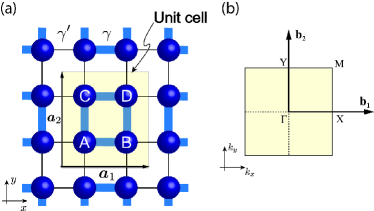
Figure 1: (a) Schematic of SSH model on square lattice. Thick and thin bonds represent the intra- and inter-cell electron hoppings, respectively. The primitive translation vector are $\bm{a_{1}}=(a,0)$ and $\bm{a_{2}}=(0,a)$. (b) Corresponding First BZ. The reciprocal lattice vector are $\bm{b_{1}}=(\frac{2\pi}{a},0)$ and $\bm{b_{2}}=(0,\frac{2\pi}{a})$.

The eigenvalue equation of 2D SSH model on square lattice is written as

$$\hat{H}(\bm{k})|u_{j}(\bm{k})\rangle=\varepsilon_{j}(\bm{k})|u_{j}(\bm{k})\rangle,$$ (1)

where $\bm{k}=(k_{x},k_{y})$ is wavenumber vector and $j(=1,2,3,4)$ is band index. Eigenvector is defined as $|u_{j}(\bm{k})\rangle=(\psi_{j,A}(\bm{k}),\psi_{j,B}(\bm{k}),\psi_{j,C}(\bm{k}),\psi_{j,D}(\bm{k}))^{T}$, where $(\cdots)^{T}$ indicates the transpose of vector. $\psi_{j,\alpha}(\bm{k})$ ($\alpha=A,B,C,D$) is the amplitude at site $\alpha$ for $j$-th energy band at $\bm{k}$. Hamiltonian $\hat{H}(\bm{k})$ is explicitly written as

$$\hat{H}(\bm{k})=\left(\begin{array}[]{cccc}0&-\rho_{x}(k_{x})&-\rho_{y}(k_{y})&0\\ -\rho_{x}^{*}(k_{x})&0&0&-\rho_{y}(k_{y})\\ -\rho_{y}^{*}(k_{y})&0&0&-\rho_{x}(k_{x})\\ 0&-\rho_{y}^{*}(k_{y})&-\rho_{x}^{*}(k_{x})&0\end{array}\right),$$ (2)

where $\rho_{l}(k_{l})=\gamma+\gamma^{\prime}\mathrm{e}^{ik_{l}a}=|\rho_{l}(k_{l})|\mathrm{e}^{i\phi_{l}(k_{l})}$ with $l=x,y$. Here, $\phi_{l}(k_{l})$ is defined as the argument of $\rho_{l}(k_{l})$ with the range of $-\pi\leq\phi_{l}(k_{l})\leq\pi$.

By solving Eq. (1), energy spectrum for bulk states are obtained as

$$\varepsilon_{j}(\bm{k})=s_{1}|\rho_{x}(k_{x})|+s_{2}|\rho_{y}(k_{y})|,$$ (3)

where $s_{1}=s_{2}=\pm 1$. The energy spectrum contains four subbands, the relations between the band index $j$ and signs $s_{1}$ and $s_{2}$ are summarized in Table 1. Eigenvectors for bulk states are obtained as

$$|u_{j}(\bm{k})\rangle=\frac{1}{2}\left(\begin{array}[]{cccc}-1\\ s_{1}\mathrm{e}^{-i\phi_{x}(k_{x})}\\ s_{2}\mathrm{e}^{-i\phi_{y}(k_{y})}\\ -s_{1}s_{2}\mathrm{e}^{-i\left[\phi_{x}(k_{x})+\phi_{y}(k_{y})\right]}\\ \end{array}\right).$$ (8)

Table 1: Relation between band index $j$, eigenvalue $\varepsilon_{j}$, eigenfunction $u_{j}$. $\zeta_{j}$ denotes the parity of eigenvector at M, X and $\Gamma$ points for trivial (nontrivial) phase.

$j$	$s_{1}$	$s_{2}$	$\varepsilon_{j}$	$u_{j}$	$\zeta_{j}$(M)	$\zeta_{j}$(X)	$\zeta_{j}$($\Gamma$)
$1$	$-$	$-$	$\varepsilon_{1}$	$u_{1}$	$+(+)$	$+(-)$	$+(+)$
$2$	$+$	$-$	$\varepsilon_{2}$	$u_{2}$	$-(-)$	$-(+)$	$-(-)$
$3$	$-$	$+$	$\varepsilon_{3}$	$u_{3}$	$-(-)$	$-(+)$	$-(-)$
$4$	$+$	$+$	$\varepsilon_{4}$	$u_{4}$	$+(+)$	$+(-)$	$+(+)$

Figures 2(a) and (b) show the energy band structures for $\gamma^{\prime}/\gamma\neq 1$ and $\gamma^{\prime}/\gamma=1$, respectively. In general, the energy band structures of 2D SSH model become identical between cases of the ratio $\gamma^{\prime}/\gamma$ and its inverse ratio $\gamma/\gamma^{\prime}$. For finite $\gamma^{\prime}/\gamma$, two band gaps open between 1st and 2nd subbands, and between 3rd and 4th subbands. The band gaps close at $\gamma^{\prime}/\gamma=1$. However, it should be noted that the parities at $\mathrm{X(Y)}$ point are inverted between two regions of $\gamma^{\prime}/\gamma\leq 1$ and $\gamma^{\prime}/\gamma>1$.

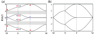
Figure 2: Energy band structure of 2D SSH model for (a) $\gamma^{\prime}/\gamma=1/3.0$ ($\gamma^{\prime}/\gamma=3.0$) and (b) $\gamma^{\prime}/\gamma=1$. The signs ($\pm$) in the plot of energy band structure represent the parity of wave function. It should be noted that band inversion occurs at X(Y) point.

The topological properties of 2D SSH model can be characterized in terms of vectored Zak phase $\bm{\mathcal{Z}}=(\mathcal{Z}_{x},\mathcal{Z}_{y})$, which is defined as the line integration of Berry connection. Berry connection for $j$-th energy band is defined as $\bm{A}_{j}=(a_{j}(k_{x}),a_{j}(k_{y}))$ with $a_{j}(k_{l})=-i\braket{u_{j}(\bm{k})}{\frac{\partial}{\partial k_{l}}}{u_{j}(\bm{k})}$. Since the band inversion happens in 2D SSH model at $\gamma^{\prime}/\gamma=1$, finite Zak phase appears for $|\gamma^{\prime}/\gamma|>1$, and absent for $|\gamma^{\prime}/\gamma|\leq 1$. In case of finite Zak phase, system possesses charge polarization which induces the TESs. From now on, we call the phase with finite Zak phase nontrivial phase, otherwise trivial phase. The $l$-th component of vectored Zak phase in 2D SSH model can be related with the winding phase of eigenvectors as

$$\mathcal{Z}_{l} = -i\sum_{j=1}^{occ.}\int_{0}^{2\pi}\braket{u_{j}(\bm{k})}{\frac{\partial}{\partial k_{l}}}{u_{j}(\bm{k})}dk_{l}$$ (9)

$$= N_{occ.}\frac{1}{2}\Delta\phi_{l}(k_{l}),$$

where $\Delta\phi_{l}(k_{l})$ is the winding phase of eigenvectors accompanied by the variation of $k_{l}$ from $0$ to $2\pi$ and $N_{occ.}$ is the number of occupied energy bands. The derivation of Eq. (9) is given in Appendix A.

Figures 3 (a) and (b) show the density plot of phase $\phi_{l}$ in trivial and nontrivial phases, respectively. In the trivial case, the magnitude of phase is almost zero everywhere in momentum space. However, in the nontrivial case, the phases $\phi_{x}$ and $\phi_{y}$ jump by $2\pi$ along the lines of $k_{x}=\pm\pi$ and $k_{y}=\pm\pi$, respectively. By looking at these figures, we can find the Zak phase as following,

$$\mathcal{Z}_{l}=\frac{1}{2}\Delta\phi_{l}(k_{l})=\begin{cases}0\ \ \ \ \ \ \ \ \ \ \gamma^{\prime}/\gamma\leq 1,\\ \pi\ \ \ \ \ \ \ \ \ \ \gamma^{\prime}/\gamma>1.\end{cases}$$ (10)

Thus, the nontrivial phase appears for $\gamma^{\prime}/\gamma>1$. The derivation of Eq. (10) is given in Appendix A.

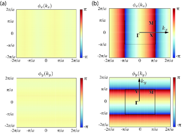
Figure 3: Density plot of the phase $\phi_{l}(k_{l})$ for (a) trivial and (b) nontrivial phases. In trivial phase, no phase jumps occurs. In nontrivial phase, however, phase jumps by $2\pi$ occur along the lines of $k_{x}=\pm\pi$ and $k_{y}=\pm\pi$, respectively.

Zak phase are related to charge polarization $\bm{P}^{j}=(P_{x}^{j},P_{y}^{j})$ as follows, King-Smith and Vanderbilt (1993); Resta (1994)

$$P_{l}^{j}=-i\frac{1}{L_{l}}\sum_{j=1}^{occ.}\sum_{k_{l}=-\pi}^{\pi}\braket{u_{j}(\bm{k})}{\frac{\partial}{\partial k_{l}}}{u_{j}(\bm{k})}=\frac{\mathcal{Z}_{l}}{2\pi}.$$ (11)

Thus, if the system has the nonzero Zak phase, charge polarization occurs, i.e. appearance of edge states. Because of $C_{4}$ symmetry, 2D SSH model has ${P}_{x}={P}_{y}$ in general. Thus, charge polarization of 2D SSH model is $\bm{P}=(0,0)$ for trivial, and $(1/2,1/2)$ for nontrivial phase, respectively.

Inversion symmetry makes a strong constraint on the value of $\bm{P}$, which is determined gauge-independently by the parities at $\Gamma$ and X (Y) points as Fang et al. (2012):

$$P_{l}^{j}=\frac{1}{2}\left(q_{l}^{j}\ \mathrm{mod}\ 2\right),$$ (12)

$$(-1)^{q_{x}^{j}}=\prod_{j\in occ.}\frac{\zeta_{j}(\mathrm{X})}{\zeta_{j}(\Gamma)}\ \ \ \ (-1)^{q_{y}^{j}}=\prod_{j\in occ.}\frac{\zeta_{j}(\mathrm{Y})}{\zeta_{j}(\Gamma)},$$ (13)

where $P_{l}^{j}$ indicates $l$-th charge polarization, and $q_{l}^{j}$ is topological invariant which is 0 or 1. The details of Eq. (12) and (13) are described in Appendix B. Thus, the value of the Zak phase determines the presence or absence of electrical polarization.

III Eigensystem of SSH Ribbons

In this section, we analytically derive the energy spectrum and corresponding wave functions of 1D SSH ribbons by using wave mechanics approach under the open boundary condition. This method has been successfully used to derive the energy spectrum and wave functions for graphene nanoribbons to show the existence of edge states. Wakabayashi et al. (2010); Wakabayashi and Dutta (2012) Explicit wave functions provide information of parity for each subbands, localization length of TES. We also inspect the topological properties of 1D SSH ribbon and crossover from one-dimensional to 2D system. In 2D limit, the topological phase transition happens when the inter- and intra-cell hoppings are equal. However, in 1D SSH ribbon, it is found that more stronger inter-cell hoppings are needed for topological phase transition owing to the finite size effect. It is also found that the critical value of transition has a power-law dependence on the ribbon width. We also show the localization length of TES for 1D SSH ribbons strongly depends on $\gamma^{\prime}/\gamma$.

Figure 4 shows schematic structure of SSH ribbon, where we assume that the lattice is translational invariant only along $y$-direction, but is finite for $x$-direction. From now on, we assume as $a=1$ for simplicity. The yellow shaded rectangle indicates unit cell of SSH ribbon, which contains $N_{x}$-plaquettes, i.e. $4\times N_{x}$ atomic orbitals in it. We call four atomic sites of $m$-th plaquette as $mA$, $mB$, $mC$ and $mD$, and define the corresponding wave functions as $\psi_{m,A}$, $\psi_{m,B}$, $\psi_{m,C}$ and $\psi_{m,D}$, where $m=0,1,\cdots,N_{x}+1$.

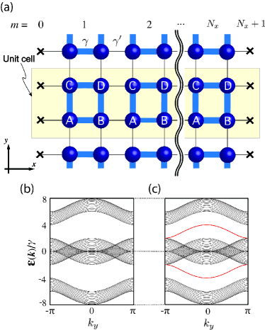
Figure 4: (a) SSH ribbon model on square lattice. $N_{x}$ is the ribbon width. The $\times$ marks indicate the missing atoms for open boundary condition. Energy band structure of $N_{x}=20$ for (b) $\gamma^{\prime}/\gamma=1/3.0$ and (c) $\gamma^{\prime}/\gamma=3.0$. In nontrivial case, edge states appear (red lines).

The equations of motion for 1D SSH ribbon is described by

$$\begin{cases}\varepsilon\psi_{m,A}=-\rho_{y}^{*}\psi_{m,C}-\gamma\psi_{m,B}-\gamma^{\prime}\psi_{m-1,B},\\ \varepsilon\psi_{m,B}=-\rho_{y}^{*}\psi_{m,D}-\gamma\psi_{m,A}-\gamma^{\prime}\psi_{m+1,A},\\ \varepsilon\psi_{m,C}=-\rho_{y}\psi_{m,A}-\gamma\psi_{m,D}-\gamma^{\prime}\psi_{m-1,D},\\ \varepsilon\psi_{m,D}=-\rho_{y}\psi_{m,B}-\gamma\psi_{m,C}-\gamma^{\prime}\psi_{m+1,C}.\end{cases}$$ (14)

The open boundary conditions for 1D SSH ribbon are given as

$$\psi_{0,B}=\psi_{0,D}=0,\psi_{N_{x}+1,A}=\psi_{N_{x}+1,C}=0.$$ (15)

Before explaining the analytic details, we shall briefly discuss the energy band structures of ribbon. Figures 4 (b) and (c) show energy band structures with $N_{x}=20$ in trivial phase with $\gamma^{\prime}/\gamma=1/3.0\leq 1$, and nontrivial phase with $\gamma^{\prime}/\gamma=3.0>1$, respectively. These band structures have been numerically obtained by solving the equations of motion. In trivial phase, gapped energy band structures are obtained. However, in nontrivial phase, doubly degenerated TESs appear inside the gaps (indicated by magenta lines).

Now let us derive the eigensystem of 1D SSH ribbons, by assuming the generic solutions of wave functions as

$$\psi_{m,\sigma}=C_{\sigma}\mathrm{e}^{ik_{x}m}+\tilde{C}_{\sigma}\mathrm{e}^{-ik_{x}m},$$ (16)

where $\sigma=A,B,C,D$. ${C}_{\sigma}$ and $\tilde{C}_{\sigma}$ are arbitrary coefficients. The open boundary condition leads to the following relations,

$$\begin{cases}\psi_{N_{x}+1,A}&=C_{A}Z+\tilde{C}_{A}Z^{-1}=0,\\ \psi_{N_{x}+1,C}&=C_{C}Z+\tilde{C}_{C}Z^{-1}=0,\\ \psi_{0,B}&=C_{B}+\tilde{C}_{B}=0,\\ \psi_{0,D}&=C_{D}+\tilde{C}_{D}=0,\end{cases}$$ (17)

where $Z=\mathrm{e}^{ik_{x}(N_{x}+1)}$. Thus we can rewrite the generic solution as

$$\begin{cases}\psi_{m,A}=C_{A}(\mathrm{e}^{ik_{x}m}-Z^{2}\mathrm{e}^{-ik_{x}m}),\\ \psi_{m,B}=C_{B}(\mathrm{e}^{ik_{x}m}-\mathrm{e}^{-ik_{x}m}),\\ \psi_{m,C}=C_{C}(\mathrm{e}^{ik_{x}m}-Z^{2}\mathrm{e}^{-ik_{x}m}),\\ \psi_{m,D}=C_{D}(\mathrm{e}^{ik_{x}m}-\mathrm{e}^{-ik_{x}m}).\end{cases}$$ (18)

By substituting these functions into the equations of motion, we obtain the secular equation for 1D SSH ribbon,

$$\bm{\hat{M}}\Psi=0,$$ (19)

where $\Psi=(C_{A},C_{B},C_{C},C_{D})^{T}$ and $\bm{\hat{M}}$ is a $4\times 4$ matrix. The matrix elements $M_{i,j}$ ($i,j=1,2,3,4$) of $\bm{\hat{M}}$ are

$$\begin{cases}M_{11}&=M_{33}=\varepsilon(\mathrm{e}^{ik_{x}m}-\mathrm{e}^{-ik_{x}m}Z^{2}),\\ M_{22}&=M_{44}=\varepsilon(\mathrm{e}^{ik_{x}m}-\mathrm{e}^{-ik_{x}m}),\\ M_{21}&=M_{43}=\rho_{x}\mathrm{e}^{ik_{x}m}-\rho_{x}^{*}\mathrm{e}^{-ik_{x}m}Z^{2},\\ M_{12}&=M_{34}=\rho_{x}^{*}\mathrm{e}^{ik_{x}m}-\rho_{x}\mathrm{e}^{-ik_{x}m},\\ M_{13}&=\rho_{y}^{*}(\mathrm{e}^{ik_{x}m}-\mathrm{e}^{-ik_{x}m}Z^{2}),\\ M_{24}&=\rho_{y}^{*}(\mathrm{e}^{ik_{x}m}-\mathrm{e}^{-ik_{x}m}),\\ M_{31}&=\rho_{y}(\mathrm{e}^{ik_{x}m}-\mathrm{e}^{-ik_{x}m}Z^{2}),\\ M_{42}&=\rho_{y}(\mathrm{e}^{ik_{x}m}-\mathrm{e}^{-ik_{x}m}),\\ M_{14}&=M_{23}=M_{32}=M_{41}=0.\end{cases}$$ (20)

It should be noted that $\Psi=0$ or $k_{x}=0,\pm\pi$ are unphysical solutions, because wave functions $\psi_{m,\sigma}$ become identically zero, i.e., electrons are absent in the system. Thus, $\mathrm{det}\bm{\hat{M}}=0$ is demanded, and leads to the following form

$$u\mathrm{e}^{4ik_{x}m}+v\mathrm{e}^{2ik_{x}m}+w+v\mathrm{e}^{-2ik_{x}m}Z^{2}+u\mathrm{e}^{-4ik_{x}m}Z^{4}=0,$$ (21)

where $u$, $v$ and $w$ are functions of $\varepsilon$, $\rho_{y}$, $\gamma$, $\gamma^{\prime}$ and $Z$. Thus, all the coefficients of $\mathrm{e}^{\pm i4k_{x}m}$, $\mathrm{e}^{\pm i2k_{x}m}$ terms and the constant term should be zero to hold Eq. (19), i.e. $u=0$, $v=0$, and $w=0$.

By using space inversion symmetry, i.e. $\psi_{N_{x}+1-m,A}=\pm\psi_{m,D}$, $\psi_{N_{x}+1-m,C}=\pm\psi_{m,B}$, we can obtain the relations $C_{D}=\pm C_{A}Z$ and $C_{B}=\pm C_{C}Z$ from Eq. (17). In addition, the mirror symmetry leads to $\psi_{m,A}=\pm\psi_{m,C}$, i.e., $C_{C}=\pm C_{A}$. Thus, the general form of the wave function can be written as

$$\left(\begin{array}[]{cccc}\psi_{m,A}\\ \psi_{m,B}\\ \psi_{m,C}\\ \psi_{m,D}\\ \end{array}\right)=N_{c}\left(\begin{array}[]{cccc}\mathrm{sin}[k_{x}(N_{x}+1-m)]\\ (-1)^{r}s_{1}\ \mathrm{sin}[k_{x}m]\\ s_{2}\ \mathrm{sin}[k_{x}(N_{x}+1-m)]\\ (-1)^{r}s_{1}s_{2}\ \mathrm{sin}[k_{x}m]\\ \end{array}\right),$$ (22)

where $r=1,2,3,\cdots,N_{x}$ indicates the band index of 1D SSH ribbon. However, as it can be clarified later, the index will be $r=1,2,3,\cdots,N_{x}-1$ in nontrivial phase, because the one missing mode will form the mode of TESs. It should be noted that the parity of wave function clearly depends on the band index $r$. $N_{c}$ is normalization constant. Owing to the translational invariance along $y$-direction, the wave function for whole ribbon system can be obtained by multiplying the Bloch phase ${\rm e}^{ik_{y}y}$ and Eq. (22).

The coefficients of $\mathrm{e}^{\pm i4k_{x}m}$ are shown to be identically zero by using the bulk energy spectrum Eq. (3), i.e.

$$u(k_{x},k_{y},N_{x}) =\varepsilon^{4}-2\varepsilon^{2}(|\rho_{x}|^{2}+|\rho_{y}|^{2})^{2}+(|\rho_{x}|^{2}-|\rho_{y}|^{2})^{2}$$

$$=\{\varepsilon^{2}-(|\rho_{x}|\pm|\rho_{y}|)^{2}\}^{2}=0.$$ (23)

Thus, $u(k_{x},k_{y},N_{x})$ is irrelevant for later discussion.

The solutions of $v=w=0$ determine the transverse wave number $k_{x}$ for a given $\gamma^{\prime}/\gamma$. Thus, we obtain

$$v(k_{x},k_{y},N_{x}) =\varepsilon^{4}[Z+Z^{-1}]$$

$$-\varepsilon^{2}[(\rho_{x}^{*2}+|\rho_{x}|^{2}+2|\rho_{y}|^{2})Z+(\rho_{x}^{2}+|\rho_{x}|^{2}+2|\rho_{y}|^{2})Z^{-1}]$$

$$+(|\rho_{x}|^{2}-|\rho_{y}|^{2})[(\rho_{x}^{*2}-|\rho_{y}|^{2})Z+(\rho_{x}^{2}-|\rho_{y}|^{2})Z^{-1}]=0,$$ (24)

$$w(k_{x},k_{y},N_{x}) =\varepsilon^{4}[Z^{2}+Z^{-2}+4]$$

$$-2\varepsilon^{2}[(\rho_{x}^{*2}+|\rho_{y}|^{2})Z^{2}+(\rho_{x}^{2}+|\rho_{y}|^{2})Z^{-2}+(\rho_{x}+\rho_{x}^{*})^{2}+4|\rho_{y}|^{2}]$$

$$+(\rho_{x}^{*2}-|\rho_{y}|^{2})^{2}Z^{2}+(\rho_{x}^{2}-|\rho_{y}|^{2})^{2}Z^{-2}+4\rho_{x}^{2}\rho_{x}^{*2}-2|\rho_{y}|^{2}(\rho_{x}+\rho_{x}^{*})^{2}+4|\rho_{y}|^{4}=0.$$ (25)

It should be noted that both $v(k_{x},k_{y},N_{x})$ and $w(k_{x},k_{y},N_{x})$ are periodic and even functions of $k_{x}$ with a period of $2\pi$, i.e. $v(k_{x},k_{y},N_{x})=v(-k_{x},k_{y},N_{x})$ and $v(k_{x}+2n\pi,k_{y},N_{x})=v(k_{x},k_{y},N_{x})$ ($n$ is arbitrary integer). Similarly, $w(k_{x},k_{y},N_{x})$ has the properties of $w(k_{x},k_{y},N_{x})=w(-k_{x},k_{y},N_{x})$ and $w(k_{x}+2n\pi,k_{y},N_{x})=w(k_{x},k_{y},N_{x})$. Thus, it is sufficient to find the solutions within the range $0<k_{x}<\pi$.

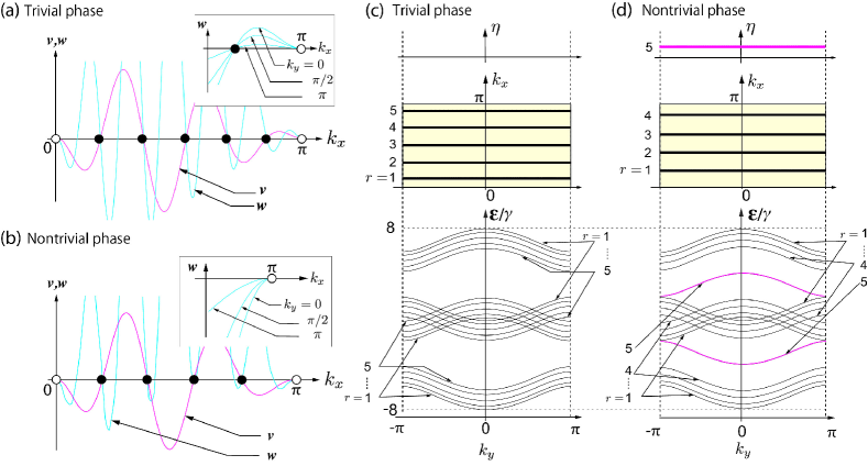
Figure 5: Schematic chart of function, $v$ (magenta line) and $w$ (cyan line) for $N_{x}=5$ in (a) trivial [$|\gamma^{\prime}/\gamma|\leq(\gamma^{\prime}/\gamma)_{c}$] and (b) nontrivial [$|\gamma^{\prime}/\gamma|>(\gamma^{\prime}/\gamma)_{c}$] phases, respectively. White circles at $k_{x}=0$ and $\pi$ are unphysical solutions. Black circle in the region of $0<k_{x}<\pi$ means real value solution of transverse wavenumber $k_{x}$. It should be noted that there are $N_{x}$ solutions for trivial phase, but only $N_{x}-1$ solutions for nontrivial phase. The insets show dependence of $w$ on longitudinal wave number $k_{y}$ near $k_{x}=\pi$. The relation between obtained complex transverse wavenumber $k_{x}+i\eta$ and corresponding energy band structure for 1D SSH model with $N_{x}=5$ for (c) trivial and (d) nontrivial phases. In the upper panels of (c) and (d), solutions of complex transverse wavenumber $k_{x}+i\eta$ in BZ are plotted. Both of $k_{x}$ and $\eta$ do not have $k_{y}$ dependence, and no imaginary part exists in trivial phase. The lower panels of (c) and (d), the corresponding energy band structures. Real value solutions ($k_{x}$) lead to energy dispersion of bulk states denoted by thin black lines, however, imaginary solution ($\eta$) leads to energy dispersion of TESs denoted by thin magenta lines.

At $\gamma^{\prime}/\gamma=1$, Eqs. (24) and (25) safely reproduce the energy spectrum of simple 2D square lattice, i.e. $\varepsilon(\bm{k})=\pm 2\gamma\left[\cos\left(\frac{k_{x}}{2}\right)\pm\cos\left(\frac{k_{y}}{2}\right)\right]$. In addition, the open boundary condition for ribbon structure leads to the transverse wave numbers $k_{x}$ as

$$k_{x}=\frac{m}{N_{x}+1}\pi,\ \ \ \ \ m=1,2,3,\cdots,N_{x}.$$ (26)

Figures 5(a) and (b) show the $k_{x}$ dependence of $u(k_{x},k_{y},N_{x})$, $v(k_{x},k_{y},N_{x})$ and $w(k_{x},k_{y},N_{x})$ for trivial and nontrivial phases, respectively. Here, we have fixed the ribbon width as $N_{x}=5$. The functions $u(k_{x},k_{y},N_{x})$, $v(k_{x},k_{y},N_{x})$ and $w(k_{x},k_{y},N_{x})$ are calculated under the condition of $\varepsilon^{2}=(|\rho_{x}|+|\rho_{y}|)^{2}$. The case of $\varepsilon^{2}=(|\rho_{x}|-|\rho_{y}|)^{2}$ is not shown, because the results do not change. The solutions of $u(k_{x},k_{y},N_{x})$, $v(k_{x},k_{y},N_{x})$ and $w(k_{x},k_{y},N_{x})$, which are denoted by black circles in Figs. 5 (a) and (b), give the transverse wavenumbers $k_{x}$ which determine the eigenstates of 1D SSH ribbon. The variation of longitudinal wavenumber $k_{y}$ only alters the amplitude of $u(k_{x},k_{y},N_{x})$, $v(k_{x},k_{y},N_{x})$ and $w(k_{x},k_{y},N_{x})$, and does not change the positions of zero points. Thus, the solutions of $\mathrm{det}\bm{M}=0$ do not depend on $k_{y}$.

For a fixed $N_{x}$, the number of real solutions $N$ for $\mathrm{det}\bm{\hat{M}}=0$ becomes different depending on the value of $\gamma^{\prime}/\gamma$, i.e.

$$N=\begin{cases}N_{x},\ \ \ \ \ \ \ \ \ \ |\gamma^{\prime}/\gamma|\leq(\gamma^{\prime}/\gamma)_{c}\\ N_{x}-1,\ \ \ \ \ |\gamma^{\prime}/\gamma|>(\gamma^{\prime}/\gamma)_{c}.\end{cases}$$ (27)

Here, $(\gamma^{\prime}/\gamma)_{c}$ is the critical value at which topological phase transition occurs. $(\gamma^{\prime}/\gamma)_{c}$ can be derived by

$$\left.\frac{\partial}{\partial k_{x}}v(k_{x},k_{y},N_{x})\right|_{k_{x}=\pi}=0.$$ (28)

In further, as indicated by Eq. (27), one real solution is missing for $|\gamma^{\prime}/\gamma|>(\gamma^{\prime}/\gamma)_{c}$. This disappearance of real solution happens near $k_{x}=\pi$ by looking at $w(k_{x},k_{y},N_{x})$ under the evolution of $\gamma^{\prime}/\gamma$, as shown in insets of Figs. 5 (a) and (b). Thus, the remaining missing solution can be obtained by analytical continuation of $k_{x}\rightarrow\pi+i\eta$. This imaginary solution $\eta$ depends on $\gamma^{\prime}/\gamma$. If $\gamma^{\prime}/\gamma$ is larger, $\eta$ also increases.

Figures 5 (c) and (d) show the relation between the obtained transverse complex wavenumber ($k_{x}+i\eta$) and energy band structures of 1D SSH ribbons with $N_{x}=5$ for trivial and nontrivial phases, respectively. In trivial phase as shown in Fig. 5 (c), no imaginary solutions appears. The real transverse wavenumbers $k_{x}$ (denoted by thick black lines) lead to the energy subbands of extended bulk states. However, in trivial phase as shown in Fig. 5 (d), an imaginary solution ($\eta$) appears, which gives the subband of TESs (thin magenta lines). Note that edge states are doubly degenerate owing to inversion symmetry.

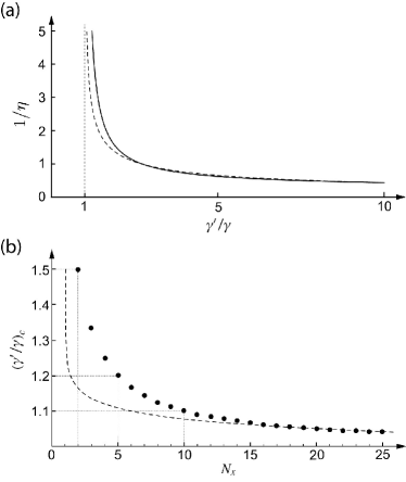
Figure 6: (a) Dependence of localization length $1/\eta$ of TES on $\gamma^{\prime}/\gamma$. Solid line is calculated from analytic wave functions of Eq. (29). Dashed line is the fitting for the large coupling limit. The fitting curve is $1/\eta=1.327(\gamma^{\prime}/\gamma-1)^{-0.481}$. (b) Ribbon width ($N_{x}$) dependence of critical value $(\gamma^{\prime}/\gamma)_{c}$, where topological phase transition occurs. In 2D limit of $N_{x}\rightarrow\infty$, $(\gamma^{\prime}/\gamma)_{c}$ converges to $1$. Black circles are $(\gamma^{\prime}/\gamma)_{c}$ obtained from Eq. (28). Dashed line is the fitting for the limit of large $N_{x}$. The fitting curve is $(\gamma^{\prime}/\gamma)_{c}=1.165(N_{x}-1)^{-0.034}$.

The wave function of TESs can be written as

$$\left(\begin{array}[]{cccc}\psi_{m,A}\\ \psi_{m,B}\\ \psi_{m,C}\\ \psi_{m,D}\\ \end{array}\right)=N_{c}\left(\begin{array}[]{cccc}\mathrm{sinh}[\eta(N_{x}+1-m)]\\ (-1)^{N_{x}}s_{1}\ \mathrm{sinh}[\eta m]\\ s_{2}\ \mathrm{sinh}[\eta(N_{x}+1-m)]\\ (-1)^{N_{x}}s_{1}s_{2}\ \mathrm{sinh}[\eta m]\\ \end{array}\right),$$ (29)

where $N_{c}$ is normalization constant. Similar to the extended states, the wave function of TESs for whole ribbon system can be obtained by multiplying the Bloch phase ${\rm e}^{ik_{y}y}$ and Eq. (29). It should be noted that the parity of TESs depends on $N_{x}$, resulting in the even-odd effect of $N_{x}$ on parity. This property can be used for band-selective filter. Nakabayashi et al. (2009) We should note that the wave function for TESs contains hyperbolic sine functions which are characterized by the imaginary transverse wavenumber $\eta$. Thus, TESs are localized states with the characteristic localization length of $1/\eta$.

Figure 6 (a) shows the electron hopping ($\gamma^{\prime}/\gamma$) dependence of the localization length ($1/\eta$). $1/\eta$ decays with the power-law on increase of $\gamma^{\prime}/\gamma$. With increase of $\gamma^{\prime}/\gamma$, the localization length of TESs becomes shorter, i.e. electrons are more strongly localized near the edges of ribbon. Thus, if the localization length is larger than ribbon width, the destructive interference between TESs from both edges occurs. In actual, this property of TESs demands that more stronger $\gamma^{\prime}/\gamma$ is necessary to induce the topological phase transition if the ribbon width gets narrower. Figure 6 (b) shows the ribbon width ($N_{x}$) dependence of $(\gamma^{\prime}/\gamma)_{c}$, which is the critical value for topological phase transition. Though $(\gamma^{\prime}/\gamma)_{c}=1$ for 2D SSH model, Figure 6 (b) shows that narrower SSH ribbons have larger $(\gamma^{\prime}/\gamma)_{c}$ than 1. Since $(\gamma^{\prime}/\gamma)_{c}$ slowly decays with increase of $N_{x}$ owing to its power-law behavior, the finite size effect persists even in the very large $N_{x}$. Thus, finite size effect for topological phase transition in 1D SSH model becomes crucial especially for narrower ribbons.

IV summary

In summary, we have analytically derived eigensystems of 2D SSH and 1D SSH ribbon models on square lattice by using wave mechanics approach. In these models, the modulation of electron hopping causes nontrivial charge polarization even in the presence of inversion symmetry. As for 2D SSH model, it has been known that the topological phase transition occurs, accompanied by nontrivial charge polarization if inter-cell hopping $\gamma^{\prime}$ are larger than intra-cell hopping $\gamma$. Owing to bulk-edge correspondence, TES are expected to appear in the nontrivial phase. However, it has been confirmed only by numerical calculations so far. In this paper, we have successfully derived full energy spectrum and corresponding wave functions for 1D SSH ribbons by using the wave mechanics approach. Mathematical relation between complex transverse wavenumber ($k_{x}+i\eta$) and energy band structures of 1D SSH ribbon are clarified. Also, the parity of wave functions and localization length of TESs are analytically identified.

It is also found that the critical value of topological phase transition $(\gamma^{\prime}/\gamma)_{c}$ strongly depends on the ribbon width and deviates from 1 which is the limit of 2D SSH model. This information will be necessary when we try to fabricate the topological electronic, photonic devices in quasi-1D geometry on the basis of SSH model.

By using the wave function used in this paper, we can discuss further electronic states of 2D SSH model subjected to other perturbations. Also, our approach is useful for constructing of Green’s functions by the decomposition of propagating and evanescent modes, which is need for atomistic calculations of electronic transport properties. Deng and Wakabayashi (2014) Our results will serve to design new 2D materials which possess non-zero Zak phase and edge states which are necessary for robust electronic transport. Furthermore, it can be applied to theory of topological photonic crystals.

F.L. is an overseas researcher under the Postdoctoral Fellowship of the Japan Society for the Promotion of Science (JSPS). K.W. acknowledges the financial support from Masuya Memorial Research Foundation of Fundamental Research. This work was supported by JSPS KAKENHI Grants No. JP17F17326, and No. JP18H01154.

Appendix A Derivation of Eqs. (9) and (10)

Here we derive the relation between Zak phase and winding phase of eigenvectors given in Eqs. (9) and (10). From eigenvector of Eq. (8), we obtain

$$\braket{u_{j}(\bm{k})}{\frac{\partial}{\partial k_{l}}}{u_{j}(\bm{k})}=\frac{i}{2}\frac{d\phi_{l}(k_{l})}{dk_{l}}.$$ (30)

Thus, Eq. (9) can be derived as

$$\mathcal{Z}_{l} = -i\sum_{j=1}^{occ.}\int_{0}^{2\pi}\braket{u_{j}(\bm{k})}{\frac{\partial}{\partial k_{l}}}{u_{j}(\bm{k})}dk_{l}$$ (31)

$$= N_{occ.}\frac{1}{2}\int_{0}^{2\pi}dk_{l}\frac{d\phi_{l}(k_{l})}{dk_{l}}$$

$$= N_{occ.}\frac{1}{2}\oint d\phi_{l}(k_{l})$$

$$\eqqcolon N_{occ.}\frac{1}{2}\Delta\phi_{l}(k_{l}),$$

where $\Delta\phi_{l}(k_{l})$ is the winding phase of eigenvectors accompanied by the variation of $k_{l}$ from $0$ to $2\pi$ and $N_{occ.}$ is the number of occupied energy bands.

From $\rho_{l}(k_{l})=|\rho_{l}(k_{l})|\mathrm{e}^{i\phi_{l}(k_{l})}$, total derivative of $\rho_{l}(k_{l})$ is obtained as

$$d\rho_{l}(k_{l})=\mathrm{e}^{i\phi_{l}(k_{l})}d|\rho_{l}(k_{l})|+i|\rho_{l}(k_{l})|\mathrm{e}^{i\phi_{l}(k_{l})}d\phi_{l}(k_{l}).$$ (32)

Identically, we have

$$\frac{1}{\rho_{l}(k_{l})}d\rho_{l}(k_{l})=\frac{1}{|\rho_{l}(k_{l})|}d|\rho_{l}(k_{l})|+id\phi_{l}(k_{l}).$$ (33)

By taking the contour integration for both sides, we obtain the winding phase of eigenvectors as

$$\frac{1}{i}\oint\frac{1}{\rho_{l}(k_{l})}d\rho_{l}(k_{l})=\Delta\phi_{l}(k_{l}),$$ (34)

where $\rho_{l}(k_{l})=\gamma^{\prime}/\gamma+\mathrm{e}^{ik_{l}}$. We should note that the integrand of the left hand side has a singular point at the origin. The path of the contour integration is a unit circle at the center $\gamma^{\prime}/\gamma$ in the complex plane, which is parameterized by $k_{l}$. Thus, we can evaluate the value of $\Delta\phi_{l}$ using residue theorem.

In trivial phase, i.e. $\gamma^{\prime}/\gamma\leq 1$, $\Delta\phi_{l}=0$, because the contour does not enclose the origin. In nontrivial phase, i.e. $\gamma^{\prime}/\gamma>1$, however, $\Delta\phi_{l}=2\pi$, because contour encloses the origin. Therefore, Zak phase in 2D SSH model is given as Eq. (10).

Appendix B Derivation of Eqs. (12) and (13)

The charge polarization can be related with the parity of wave functions. In order to show the relation, let us define the sewing matrix $\omega$, which is in form of the space inversion operator $\Pi$ for formulation of Zak phase for multi-band system. Here, $\Pi$ an operator that inverts position as $\Pi u(\bm{k})=u(\bm{-k})$. The sewing matrix $\omega$ is define as

$$\omega_{ij}(\bm{k})\coloneqq\braket{u_{i}(-\bm{k})}{\Pi}{u_{j}(\bm{k})},$$ (35)

which $i,j$ are band index. In addition, we define Berry connection matrix as $\bm{a}_{ij}(\bm{k})=-i\braket{u_{i}(\bm{k})}{\nabla_{\bm{k}}}{u_{j}(\bm{k})}$. By using this matrix, Eq. (11) can be rewritten as

$$P_{l} = \sum_{j=1}^{occ.}\int_{-\pi}^{\pi}\frac{dk_{l}}{2\pi}a_{jj}(k_{l})$$ (36)

$$= \frac{1}{2\pi}\int_{-\pi}^{\pi}dk_{l}\ \mathrm{Tr}[\bm{a}_{ij}(k_{l})].$$

In the presence of space inversion symmetry, the integrand of Eq. (36) can be rewritten as

$$\mathrm{Tr}[\bm{a}_{ij}(\bm{k})]=\mathrm{Tr}[\bm{a}_{ij}(-\bm{k})]+i\mathrm{Tr}[\omega_{ij}^{\dagger}(\bm{k})\nabla_{\bm{k}}\omega_{ij}(\bm{k})].$$

Therefore, charge polarization is expressed as

$$P_{l} = \frac{1}{2\pi}\int_{-\pi}^{\pi}dk_{l}\ \left\{\mathrm{Tr}[\bm{a}(-\bm{k})]+i\mathrm{Tr}[\omega^{{\dagger}}(\bm{k})\frac{\partial}{\partial k_{l}}\omega(\bm{k})]\right\}$$

$$= -P_{l}+q_{l}^{j}.$$

Here, $q_{l}^{j}$ is right hand of integral element. Using the unitarity of $\omega(\bm{k})$, the integrand of $q_{x}^{j}$ can be rewritten as $\mathrm{Tr}[\omega^{\dagger}(\bm{k})\nabla_{k}\omega(\bm{k})]=\nabla_{k}\mathrm{log}(\mathrm{det}[\omega(\bm{k})])$. Thus, we obtain

$$q_{x}^{j} = -\frac{i}{2\pi}\int_{-\pi}^{\pi}dk_{l}\frac{d\mathrm{ln}(\mathrm{det}[\omega(k_{x},0)])}{dk_{l}}$$ (37)

$$= -\frac{i}{\pi}\mathrm{ln}\left\{\frac{\mathrm{det}[\omega(\pi,0)]}{\mathrm{det}[\omega(0,0)]}\right\}.$$

Since eigenvalue of space inversion operator $\Pi$ is $\pm 1$, $\mathrm{det}[\omega(\bm{k})]$ is given as

$$\mathrm{det}[\omega(\bm{k})]=\prod_{j\in occ.}\zeta_{j}(\bm{k}),$$ (38)

where $\zeta_{j}(\bm{k})$ are the parity of wave function in $j$-th energy band at $\bm{k}$. Substituting Eq. (38) into Eq. (37) leads to

$$\mathrm{ln}(\mathrm{e}^{i\pi q_{x}^{j}}) =\mathrm{ln}\left\{\prod_{j\in occ.}\frac{\zeta_{j}(\pi,0)}{\zeta_{j}(0,0)}\right\},$$

$$(-1)^{q_{x}^{j}} =\prod_{j\in occ.}\frac{\zeta_{j}(\mathrm{X})}{\zeta_{j}(\Gamma)}.$$ (39)

Similarly, $y$ component is also obtained by replacing $\mathrm{X}$ with $\mathrm{Y}$. Thus $q_{l}^{j}$ is topological invariant, which gives either 0 or 1.

References

- Bansil et al. (2016) A. Bansil, H. Lin, and T. Das, Rev. Mod. Phys. 88, 021004 (2016).
- Hasan and Kane (2010) M. Z. Hasan and C. L. Kane, Rev. Mod. Phys. 82, 3045 (2010).
- Qi and Zhang (2011) X.-L. Qi and S.-C. Zhang, Rev. Mod. Phys. 83, 1057 (2011).
- Kane and Mele (2005) C. L. Kane and E. J. Mele, Phys. Rev. Lett. 95, 226801 (2005).
- Bernevig et al. (2006) B. A. Bernevig, T. L. Hughes, and S.-C. Zhang, Science 314, 1757 (2006).
- Fu et al. (2007) L. Fu, C. L. Kane, and E. J. Mele, Phys. Rev. Lett. 98, 106803 (2007).
- Hsieh et al. (2008) D. Hsieh, D. Qian, L. Wray, Y. Xia, Y. S. Hor, R. J. Cava, and M. Z. Hasan, Nature 452, 970 (2008).
- Chen et al. (2009) Y. L. Chen, J. G. Analytis, J.-H. Chu, Z. K. Liu, S.-K. Mo, X. L. Qi, H. J. Zhang, D. H. Lu, X. Dai, Z. Fang, S. C. Zhang, I. R. Fisher, Z. Hussain, and Z.-X. Shen, Science 325, 178 (2009).
- Chang et al. (2013) C.-Z. Chang, J. Zhang, X. Feng, J. Shen, Z. Zhang, M. Guo, K. Li, Y. Ou, P. Wei, L.-L. Wang, Z.-Q. Ji, Y. Feng, S. Ji, X. Chen, J. Jia, X. Dai, Z. Fang, S.-C. Zhang, K. He, Y. Wang, L. Lu, X.-C. Ma, and Q.-K. Xue, Science 340, 167 (2013).
- Ando (2013) Y. Ando, J. Phys. Soc. Jpn. 82, 102001 (2013).
- Sato and Fujimoto (2016) M. Sato and S. Fujimoto, J. Phys. Soc. Jpn. 85, 072001 (2016).
- Fu (2011) L. Fu, Phys. Rev. Lett. 106, 106802 (2011).
- Tanaka et al. (2012) Y. Tanaka, Z. Ren, T. Sato, K. Nakayama, S. Souma, T. Takahashi, K. Segawa, and Y. Ando, Nat. Phys. 8, 800 (2012).
- Dziawa et al. (2012) P. Dziawa, B. J. Kowalski, K. Dybko, R. Buczko, A. Szczerbakow, M. Szot, E. Łusakowska, T. Balasubramanian, B. M. Wojek, M. H. Berntsen, O. Tjernberg, and T. Story, Nat. Mater. 11, 1023 (2012).
- Ando and Fu (2015) Y. Ando and L. Fu, Annu. Rev. Condens. Matter Phys. 6, 361 (2015).
- Wan et al. (2011) X. Wan, A. M. Turner, A. Vishwanath, and S. Y. Savrasov, Phys. Rev. B 83, 205101 (2011).
- Burkov and Balents (2011) A. A. Burkov and L. Balents, Phys. Rev. Lett. 107, 127205 (2011).
- Borisenko et al. (2014) S. Borisenko, Q. Gibson, D. Evtushinsky, V. Zabolotnyy, B. Büchner, and R. J. Cava, Phys. Rev. Lett. 113, 027603 (2014).
- Liang et al. (2016) Q.-F. Liang, J. Zhou, R. Yu, Z. Wang, and H. Weng, Phys. Rev. B 93, 085427 (2016).
- Watanabe et al. (2016) H. Watanabe, H. C. Po, M. P. Zaletel, and A. Vishwanath, Phys. Rev. Lett. 117, 096404 (2016).
- Kobayashi et al. (2016) S. Kobayashi, Y. Yanase, and M. Sato, Phys. Rev. B 94, 134512 (2016).
- Yang et al. (2017) B.-J. Yang, T. A. Bojesen, T. Morimoto, and A. Furusaki, Phys. Rev. B 95, 075135 (2017).
- Liu and Wakabayashi (2019) F. Liu and K. Wakabayashi, Jpn. J. Appl. Phys. 58 (2019).
- Liu and Wakabayashi (2017) F. Liu and K. Wakabayashi, Phys. Rev. Lett. 118, 076803 (2017).
- Zak (1989) J. Zak, Phys. Rev. Lett. 62, 2747 (1989).
- King-Smith and Vanderbilt (1993) R. D. King-Smith and D. Vanderbilt, Phys. Rev. B 47, 1651 (1993).
- Resta (1994) R. Resta, Rev. Mod. Phys. 66, 899 (1994).
- Zhou et al. (2015) Y. Zhou, K. M. Rabe, and D. Vanderbilt, Phys. Rev. B 92, 041102(R) (2015).
- Hirayama et al. (2018) M. Hirayama, S. Matsuishi, H. Hosono, and S. Murakami, Phys. Rev. X 8, 031067 (2018).
- Huang et al. (2018) H. Huang, K.-H. Jin, S. Zhang, and F. Liu, Nano Lett. 18, 1972 (2018).
- Liu et al. (2017a) F. Liu, M. Yamamoto, and K. Wakabayashi, J. Phys. Soc. Jpn. 86, 123707 (2017a).
- Kameda et al. (2019) T. Kameda, F. Liu, S. Dutta, and K. Wakabayashi, Phys. Rev. B 99, 075426 (2019).
- Benalcazar et al. (2017a) W. A. Benalcazar, B. A. Bernevig, and T. L. Hughes, Science 357, 61 (2017a).
- Benalcazar et al. (2017b) W. A. Benalcazar, B. A. Bernevig, and T. L. Hughes, Phys. Rev. B 96, 245115 (2017b).
- Song et al. (2017) Z. Song, Z. Fang, and C. Fang, Phys. Rev. Lett. 119, 246402 (2017).
- Fukui and Hatsugai (2018) T. Fukui and Y. Hatsugai, Phys. Rev. B 98, 035147 (2018).
- Wang et al. (2018) Z. Wang, B. J. Wieder, J. Li, B. Yan, and B. A. Bernevig, “Higher-order topology, monopole nodal lines, and the origin of large fermi arcs in transition metal dichalcogenides xte2 (x=mo,w),” (2018), arXiv:1806.11116 .
- Ezawa (2018) M. Ezawa, Phys. Rev. Lett. 120, 026801 (2018).
- Liu et al. (2019a) F. Liu, H.-Y. Deng, and K. Wakabayashi, Phys. Rev. Lett. 122, 086804 (2019a).
- Yoshida et al. (2019) A. Yoshida, Y. Ohtaki, R. Ohtaki, and T. Fukui, “Edge states, corner states, and flat bands in a two-dimensional pt symmetric system,” (2019), arXiv:1904.05007 .
- Liu et al. (2018) F. Liu, H.-Y. Deng, and K. Wakabayashi, Phys. Rev. B 97, 035442 (2018).
- Xiao et al. (2014) M. Xiao, Z. Q. Zhang, and C. T. Chan, Phys. Rev. X 4, 021017 (2014).
- Xie et al. (2018) B.-Y. Xie, H.-F. Wang, H.-X. Wang, X.-Y. Zhu, J.-H. Jiang, M.-H. Lu, and Y.-F. Chen, Phys. Rev. B 98, 205147 (2018).
- Chen et al. (2018) X.-D. Chen, W.-M. Deng, F.-L. Shi, F.-L. Zhao, M. Chen, and J.-W. Dong, “Direct observation of corner states in second-order topological photonic crystal slabs,” (2018), arXiv:1812.08326 .
- Ota et al. (2019) Y. Ota, F. Liu, R. Katsumi, K. Watanabe, K. Wakabayashi, Y. Arakawa, and S. Iwamoto, Optica 6, 786 (2019).
- Liu et al. (2017b) Y. Liu, C.-S. Lian, Y. Li, Y. Xu, and W. Duan, Phys. Rev. Lett. 119, 255901 (2017b).
- Zhang et al. (2018) X. Zhang, Z.-K. Lin, H.-X. Wang, Z. Xiong, Y. Tian, M.-H. Lu, Y.-F. Chen, and J.-H. Jiang, “Hierarchical multipole topological insulators,” (2018), arXiv:1811.05514 .
- Zhang et al. (2019) Z. Zhang, M. Rosendo López, Y. Cheng, X. Liu, and J. Christensen, Phys. Rev. Lett. 122, 195501 (2019).
- Zheng et al. (2019) L.-Y. Zheng, V. Achilleos, O. Richoux, G. Theocharis, and V. Pagneux, “Observation of edge waves in a two-dimensional su-schrieffer-heeger acoustic network,” (2019), arXiv:1903.11961 .
- Liu et al. (2019b) S. Liu, W. Gao, Q. Zhang, S. Ma, L. Zhang, C. Liu, Y. Xiang, T. Cui, and S. Zhang, Research 2019 (2019b), 10.1155/2019/8609875.
- Su et al. (1980) W. P. Su, J. R. Schrieffer, and A. J. Heeger, Phys. Rev. B 22, 2099 (1980).
- Heeger et al. (1988) A. J. Heeger, S. Kivelson, J. R. Schrieffer, and W. P. Su, Rev. Mod. Phys. 60, 781 (1988).
- Fujita et al. (1996) M. Fujita, K. Wakabayashi, K. Nakada, and K. Kusakabe, J. Phys. Soc. Jpn. 65, 1920 (1996).
- Nakada et al. (1996) K. Nakada, M. Fujita, G. Dresselhaus, and M. S. Dresselhaus, Phys. Rev. B 54, 17954 (1996).
- Wakabayashi et al. (1999) K. Wakabayashi, M. Fujita, H. Ajiki, and M. Sigrist, Phys. Rev. B 59, 8271 (1999).
- Delplace et al. (2011) P. Delplace, D. Ullmo, and G. Montambaux, Phys. Rev. B 84, 195452 (2011).
- Rizzo et al. (2018) D. J. Rizzo, G. Veber, T. Cao, C. Bronner, T. Chen, F. Zhao, H. Rodriguez, S. G. Louie, M. F. Crommie, and F. R. Fischer, Nature 560, 204 (2018).
- Gröning et al. (2018) O. Gröning, S. Wang, X. Yao, C. A. Pignedoli, G. B. Barin, C. Daniels, A. Cupo, V. Meunier, X. Feng, A. Narita, K. Müllen, P. Ruffieux, and R. Fasel, Nature 560, 209 (2018).
- Wakabayashi et al. (2007) K. Wakabayashi, Y. Takane, and M. Sigrist, Phys. Rev. Lett. 99, 036601 (2007).
- Wakabayashi et al. (2009a) K. Wakabayashi, Y. Takane, M. Yamamoto, and M. Sigrist, New J. Phys. 11, 095016 (2009a).
- Wakabayashi et al. (2009b) K. Wakabayashi, Y. Takane, M. Yamamoto, and M. Sigrist, Carbon 47, 124 (2009b).
- Baringhaus et al. (2014) J. Baringhaus, M. Ruan, F. Edler, A. Tejeda, M. Sicot, A. Taleb-Ibrahimi, A.-P. Li, Z. Jiang, E. H. Conrad, C. Berger, C. Tegenkamp, and W. A. d. Heer, Nature 506, 349 (2014).
- Wakabayashi et al. (2010) K. Wakabayashi, K.-i. Sasaki, T. Nakanishi, and T. Enoki, Sci. Tecnol. Adv. Mat 11, 054504 (2010).
- Wakabayashi and Dutta (2012) K. Wakabayashi and S. Dutta, Solid State Communications 152, 1420 (2012), exploring Graphene, Recent Research Advances.
- Fang et al. (2012) C. Fang, M. J. Gilbert, and B. A. Bernevig, Phys. Rev. B 86, 115112 (2012).
- Nakabayashi et al. (2009) J. Nakabayashi, D. Yamamoto, and S. Kurihara, Phys. Rev. Lett. 102, 066803 (2009).
- Deng and Wakabayashi (2014) H.-Y. Deng and K. Wakabayashi, Phys. Rev. B 90, 045402 (2014).