Search with home returns provides advantage under high uncertainty

Abstract

Many search processes are conducted in the vicinity of a favored location, i.e., a home, which is visited repeatedly. Foraging animals return to their dens and nests to rest, scouts return to their bases to resupply, and drones return to their docking stations to recharge or refuel. Yet, despite its prevalence, very little is known about search with home returns as its analysis is much more challenging than that of unconstrained, free-range, search. Here, we develop a theoretical framework for search with home returns. This makes no assumptions on the underlying search process and is furthermore suited to treat generic return and home-stay strategies. We show that the solution to the home-return problem can then be given in terms of the solution to the corresponding free-range problem—which not only reduces overall complexity but also gives rise to a simple, and universal, phase-diagram for search. The latter reveals that search with home returns outperforms free-range search in conditions of high uncertainty. Thus, when living gets rough, a home will not only provide warmth and shelter but also allow one to locate food and other resources quickly and more efficiently than in its absence.

I Introduction

Consider a falcon roaming the sky in search of prey well hidden amongst the grass below. The falcon will wander around for a while, but if prey is not found it will eventually return to its nest empty-handed. Other animals—humans included—display similar behaviour while foraging and when engaged in search activities HR1 ; HR2 ; HR3 ; and home-return capabilities are now routinely built into robots and drones to avoid running out of fuel or battery power. However, while the observation that most natural search processes are home-bound goes back to Darwin Darwin , it is still unclear if this situation merely reflects the prevalence of permanent dwellings, or rather is a result of evolutionary convergence to a superior search strategy. To start answering this question, one must first understand how being home-bound affects search and the time it takes to locate a target. In what follows, we analyze this problem and characterize precisely under which circumstances having a home allows one to locate food and other resources quickly and more efficiently than in its absence.

A free-range searcher will set off from a certain location and look for a target until it is found. In contrast, search with home returns is a cyclic process which consists of three stages: search, return, and home (Fig. 1A). How much time does it take such a searcher to find its target? At face value, it seems that this question can be answered by taking advantage of the existing theory of search Search1 ; Search2 ; Search3 ; Search4 ; Search5 ; Search6 ; Search7 ; Search8 and first-passage FPT1 ; FPT2 ; FPT3 ; FPT4 ; FPT5 ; FPT6 ; FPT7 ; FPT8 , and of recent advancements in our understanding of first-passage under restart Restart-ND-0 ; Restart-ND-1 ; Restart-ND-2 ; Restart-ND-3 ; Restart-ND-4 ; Restart-ND-5 ; Restart-ND-6 ; Restart-ND-7 ; Restart-ND-8 ; Restart-ND-9 ; Restart-ND-10 ; Restart-D-0 ; Restart-D-1 ; Restart-D-2 ; Restart-D-3 ; Restart-D-4 ; Restart-D-5 ; Restart-D-6 ; Restart-D-7 ; Restart-D-8 . Indeed, search with home returns can be seen as a regular first-passage process that is restarted by home returns. However, basic models of first-passage under restart are a far cry from reality as they assume that home-returns are instantaneous and that home-stays can also be neglected Restart-ND-0 ; Restart-ND-1 ; Restart-ND-2 ; Restart-ND-3 ; Restart-ND-4 ; Restart-ND-5 ; Restart-ND-6 ; Restart-ND-7 ; Restart-ND-8 ; Restart-ND-9 ; Restart-ND-10 .

More sophisticated models of search with home returns lump together return and home-stay times assuming that the search stage is followed by some generic delay Restart-D-0 ; Restart-D-1 ; Restart-D-2 ; Restart-D-3 ; Restart-D-4 ; Restart-D-5 ; Restart-D-6 ; Restart-D-7 . This is a step in the right direction: it takes time to get from one place to another, and time spent home to e.g., recover, recharge, or refuel, may not be negligible. However, the time it takes a searcher to return home will typically depend on the distance home, as places that are further away take more time to be reached. Yet, this basic physics is clearly ignored when assuming that the delay which follows the search stage is generic and independent of the searcher’s position as it starts heading back home return1 ; return2 ; return3 ; return4 ; return5 . This non-realistic modelling assumption is in many ways similar to the complete decoupling between waiting time and jump length in the continuous time random walk (CTRW) model CTRW1 ; CTRW2 ; CTRW3 ; CTRW4 . In the latter case, the problem was solved by the development of space-time coupled CTRWs SPC-CTRW and Lévy walks Walks-CTRW1 ; Walks-CTRW2 ; Walks-CTRW3 ; Walks-CTRW4 ; Walks-CTRW5 ; Walks-CTRW6 which introduced explicit correlations between time and distance traveled. In what follows, we take a similar approach and build a space-time coupled theory for first-passage under restart. This, in turn, will be used to describe search with home returns.

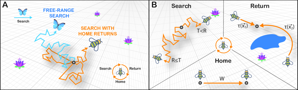
Figure 1: A. Free-range search vs. search with home returns. The butterfly (free-range searcher) and the bee (searcher with home returns) set off in search of a flower (target). The butterfly, which has no permanent dwellings, will look for a flower until it finds one. In contrast, if the bee is unable to find a flower it will return to its hive, spend some time there, and start searching again at a later occasion. B. Search with home returns is a cyclic, three stage, process. In the search stage a target is sought for a time that is the minimum of the free-range FPT, $T$, and the restart time $R$. If $T<R$, a target is found and the search ends. Conversely, if $R\leq T$, no target is found and the searcher heads back home. The duration of the return stage, $\tau(\vec{x})$, is determined by the searcher’s position $\vec{x}$ at the end of the search phase. This stage ends when the searcher is back home. In the home stage the searcher stays home for a time $W$.

The paper is structured as follows. In Secs. II and III, we develop a theoretical framework for search with home returns. We show that this framework provides a practical analysis tool as it allows one to provide the solution to the home return problem in terms of the solution to the corresponding problem without home returns. This useful property is demonstrated in Sec. IV with the example of diffusive search. In Sec. V, we build on our framework to reveal a universal phase diagram for search. In particular, we show that search with home returns is preferable in conditions of high uncertainty as it can then reduce the mean time taken to locate a target. This property is illustrated with the example of drift-diffusive search in Sec. VI. In Sec. VII, we show that search with home returns can also reduce fluctuations in the time taken to locate a target. This feature is illustrated with the example of Lévy search in Sec. VIII and its importance is discussed. Conclusions and outlook are given in Sec. IX. Some details and derivations are relegated to the appendix.

II A theoretical framework for search with home returns

Consider a searcher that starts at the origin (home) of a (possibly infinite) $d$-dimensional arena at time zero. In the absence of home returns, the searcher will locate one of the existing targets in the arena following a random time $T$. This time is a property of the free-range problem, and we will henceforth refer to it as the free-range first-passage time (FPT). We will not make any assumptions on the arena, the search process, and target distribution that govern $T$. However, and in contrast to free-range search, here we will consider a situation where the searcher returns home if it fails to locate the target within a time $R$ (can be random) which we will henceforth refer to as the restart time. Thus, if $T<R$ the searcher finds the target before it is required to return and the search process completes. Otherwise, the searcher will stop looking for the target and start its return back home (Fig. 1B - Search).

The time it takes the searcher to return home will typically depend on the searcher’s position at the end of the search stage (Fig. 1B - Return). For example, the searcher may return home by moving at a constant speed along the shortest possible path. The return time is then simply given by the distance to home over the speed of travel. However, various constraints, e.g., topographic ones, may force the searcher to follow a different route and may also affect its velocity. Such situations will result in more complicated relations between the position of the searcher and its return time. To capture this, we allow the return time $\tau(\vec{x})$ to be a general function of the searcher’s position $\vec{x}$. After the searcher returns home it stays there for some generic time $W$ which can also be random (Fig. 1B - Home). This, search–return–home, cycle repeats itself until a target is found at some point during the search stage. In what follows, we will assume that targets cannot be located during the return and home phases (see discussion in Sec. IX).

The above description allows us to write a renewal equation for the FPT of search with home returns, which is the time it takes the searcher to locate a target. Denoting this time by $T_{R}$, we have

$$\begin{array}[]{l}T_{R}=\left\{\begin{array}[]{lll}T&&\text{if ~{}~{}}T<R\text{ ,}\\ &\text{ \ \ }\\ R+\tau(\vec{x})+W+T_{R}^{\prime}&&\text{if~{}~{} }R\leq T\text{ ,}\end{array}\right.\text{ }\end{array}$$ (1)

where $T$, $R$, $\tau(\vec{x})$, and $W$ were defined above; and $T_{R}^{\prime}$ is an independent and identically distributed copy of $T_{R}$. Taking expectations in Eq. (1), we obtain (Appendix A)

$$\langle T_{R}\rangle=\underbrace{\frac{\langle\text{min}(T,R)\rangle}{\text{Pr}(T<R)}}_{\text{search}}+\underbrace{\frac{\langle I(R\leq T)\tau(\vec{x})\rangle}{\text{Pr}(T<R)}}_{\text{return}}+\underbrace{\frac{\text{Pr}(R\leq T)\langle W\rangle}{\text{Pr}(T<R)}}_{\text{home}},$$ (2)

where $I(R\leq T)$ is an indicator function which takes the value one if $R\leq T$, i.e., with probability $\text{Pr}(R\leq T)$, and is zero otherwise; and different contributions to the sum are labeled according to their source.

The first term on the right-hand side of Eq. (2) gives the FPT of the searcher in an idealized scenario where return and home times can be neglected ($\tau(\vec{x})=0$, $W=0$) Restart-ND-5 . The second term gets its contribution from the time it takes the searcher to return home and the third term comes from the time spent at home. Evaluating the first and third terms is straightforward given the probability distributions of $R,~{}T$, and $W$ (Appendix B). The second term is slightly more delicate because it depends on $\vec{x}$—the random position of the searcher at the end of the search stage. To evaluate this term, we let $f_{R}(t)$ denote the probability density function of the restart time $R$. We then observe that

$$\langle I(R\leq T)\tau(\vec{x})\rangle =\int_{0}^{\infty}dtf_{R}(t)~{}\langle\tau(\vec{x}(t))I(R\leq T)|R=t\rangle$$

$$=\int_{0}^{\infty}dtf_{R}(t)\text{Pr}(T\geq t)\langle\tau(\vec{x}(t))\big{|}R=t,T\geq t\rangle,$$ (3)

where we have first conditioned on restart happening at time $t$, and then on $T$ being either smaller or larger than this time. Note that a non-zero contribution is obtained only for $T\geq t$, i.e., only when the target is not found and a return actually takes place.

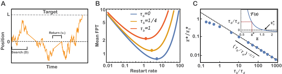
Figure 2: A. An illustration of diffusive search with home returns. B. The mean FPT, $\langle T_{r}\rangle$, from Eq. (9) vs. the restart rate $r$. Here, $\tau_{d}=1/2$ and results are shown for different values of $\tau_{b}$ [see Eq. (10)]. C. The scaled optimal restart rate, $r^{*}/r_{0}^{*}$, obtained from a minimization of Eq. (9) vs. $\tau_{b}/\tau_{d}$. The scaling predicted by Eq. (12) is seen to hold. Inset. $\mathcal{F}(z)$ from Eq. (11) vs. $z$. The ratio $\tau_{b}/\tau_{d}$ sets the solution $z^{*}$.

In order to proceed, we define the free-range propagator, $G_{0}(\vec{x},t)$, as the probability density to find the searcher at position $\vec{x}$ at time $t$ given that it started at the origin. Note that this propagator is called free-range because it is defined in the presence of targets but in the absence of home-returns. Thus, the free-range survival probability is given by $\text{Pr}(T\geq t)=\int_{\mathcal{D}}d\vec{x}~{}G_{0}(\vec{x},t)$, where $\mathcal{D}$ is the available search domain. The internal expectation in Eq. (3) can then be written as $\langle\tau(\vec{x}(t))\big{|}R=t,~{}T\geq t\rangle=\frac{1}{\text{Pr}(T\geq t)}\int_{\mathcal{D}}~{}d\vec{x}~{}\tau(\vec{x})~{}G_{0}(\vec{x},t)$. Substituting this expression into Eq. (3), we obtain

$$\langle I(R\leq T)\tau(\vec{x})\rangle=\int_{0}^{\infty}dt~{}f_{R}(t)\int_{\mathcal{D}}d\vec{x}~{}\tau(\vec{x})~{}G_{0}(\vec{x},t)~{}.$$ (4)

Equation (4) asserts that the second term in Eq. (2) can be evaluated given the free-range propagator $G_{0}(\vec{x},t)$, which in turn allows full evaluation of the mean FPT.

Starting from Eq. (1), and proceeding similarly to the above, the distribution of the FPT, $T_{R}$, can also be determined. Letting $\tilde{T}_{R}(s)=\langle e^{-sT_{R}}\rangle$ stand for the Laplace transform of the latter, we find (Appendix C)

$$\tilde{T}_{R}(s)=\frac{\text{Pr}(T<R)\tilde{T}_{\text{min}}(s)}{1-\tilde{W}(s)\int_{0}^{\infty}~{}dt~{}f_{R}(t)e^{-st}~{}\int_{\mathcal{D}}~{}d\vec{x}~{}e^{-s\tau(\vec{x})}~{}G_{0}(\vec{x},t)}~{},$$

(5)

with $\tilde{W}(s)=\langle e^{-sW}\rangle$ standing for the Laplace transform of $W$, and $\tilde{T}_{\text{min}}(s)=\langle e^{-sT_{\text{min}}}\rangle$ standing for the Laplace transform of the random variable $T_{\text{min}}=\{T|T<R\}$ whose density is given by $f_{T_{\text{min}}}(t)=\frac{f_{T}(t)\int_{t}^{\infty}~{}dt^{\prime}~{}f_{R}(t^{\prime})}{\text{Pr}(T<R)}=\frac{f_{T}(t)\text{Pr}(R>t)}{\text{Pr}(T<R)}~{}$. Equation (5) asserts that the distribution of $T_{R}$ can be determined given the free-range propagator $G_{0}(\vec{x},t)$, and the random variables $R$ and $W$. In addition, all the moments can be computed using the formula $\langle T_{R}^{n}\rangle=(-1)^{n}\frac{d^{n}}{ds^{n}}\tilde{T}_{R}(s)|_{s=0}$.

III Exponential restart times

So far, we have made no assumptions on the distribution of the time $R$ which governs restart. In what follows, we show that much insight can be gained by focusing on the case where $R$ is exponentially distributed with rate $r$. Letting $\tilde{G}_{0}(\vec{x},r)=\int_{0}^{\infty}~{}dt~{}e^{-rt}~{}G_{0}(\vec{x},t)$ and $\tilde{T}(r)=\int_{0}^{\infty}~{}dt~{}e^{-rt}~{}f_{T}(t)=1-r\int_{\mathcal{D}}d\vec{x}~{}\tilde{G}_{0}(\vec{x},r)$ stand respectively for the Laplace transforms of $G_{0}(\vec{x},t)$ and $f_{T}(t)$ evaluated at $r$, we find that in this case Eq. (2) boils down to (Appendix D)

$$\langle T_{r}\rangle=\underbrace{\frac{1-\tilde{T}(r)}{r\tilde{T}(r)}}_{\text{search}}+\underbrace{\frac{1-\tilde{T}(r)}{\tilde{T}(r)}\langle\tau(\vec{x})\rangle_{r}}_{\text{return}}+\underbrace{\frac{1-\tilde{T}(r)}{\tilde{T}(r)}\langle W\rangle}_{\text{home}},$$ (6)

where $\langle\tau(\vec{x})\rangle_{r}\equiv\int_{\mathcal{D}}~{}d\vec{x}~{}\tau(\vec{x})~{}\phi_{r}(\vec{x})$ is the mean return time taken with respect to the probability measure $\phi_{r}(\vec{x})=\tilde{G}_{0}(\vec{x},r)/\int_{\mathcal{D}}d\vec{x}~{}\tilde{G}_{0}(\vec{x},r)$. Similarly, the expression for the FPT distribution can also be simplified to read (Appendix E)

$$\tilde{T}_{r}(s)=\frac{\tilde{T}(s+r)}{1-r~{}\tilde{W}(s)~{}\int_{\mathcal{D}}~{}d\vec{x}~{}e^{-s\tau(\vec{x})}~{}\tilde{G}_{0}(\vec{x},s+r)}.$$ (7)

From Eq. (7) we see that the distribution of $T_{r}$ can always be written in terms of the Laplace transforms of the free-range propagator $G_{0}(\vec{x},t)$, and the random variables $T$ and $W$.

IV Diffusive search with home returns

To illustrate how the framework developed above can be utilized in practice, we examine a paradigmatic case study. Consider a 1-d search process in which a particle that starts at the origin diffuses until it hits a stationary target; and let $D$ and $L$ denote respectively the diffusion constant and the initial distance from the target. In addition, assume that the process is restarted at a constant rate $r$ upon which the searcher returns home at a constant speed $v_{r}$ (Fig. 2A). In what follows, the time spent home will be neglected as its stand-alone contribution is already well-understood Restart-D-0 ; Restart-D-1 ; Restart-D-2 ; Restart-D-3 ; Restart-D-4 ; Restart-D-5 ; Restart-D-6 ; Restart-D-7 .

To progress, we recall that the free-range propagator of this problem is given by FPT1

$$G_{0}(x,t)=\frac{1}{\sqrt{4\pi Dt}}\left(e^{-\frac{x^{2}}{4Dt}}-e^{-\frac{(2L-x)^{2}}{4Dt}}\right)~{}.$$ (8)

To get the mean FPT with home returns, we observe that the time penalty due to a ballistic home-return from position $x$ is given by $\tau(x)=|x|/v_{r}$. Plugging in the above into Eq. (6) gives (Appendix F)

$$\langle T_{r}\rangle=\underbrace{\frac{1}{r}\left(e^{\sqrt{\tau_{d}r}}-1\right)}_{\text{search}}+\underbrace{\tau_{b}~{}\left[\frac{2\sinh(\sqrt{\tau_{d}r})}{\sqrt{\tau_{d}r}}-1\right]}_{\text{return}}~{},$$ (9)

where

$$\tau_{d}=\frac{L^{2}}{D}~{}\text{,~{}~{}~{}and}~{}~{}~{}\tau_{b}=\frac{L}{v_{r}}~{},$$ (10)

stand respectively for the diffusive and ballistic time scales in the problem.

In the limit $\tau_{b}\to 0$, Eq. (9) boils down to the classical result for the mean FPT of diffusion with resetting Restart-ND-1 , but we would now like to understand the effect of non instantaneous and space-time-coupled home returns. In Fig. 2B, we plot $\langle T_{r}\rangle$ as a function of the restart rate for $\tau_{d}=1/2$ and different values of $\tau_{b}$ (see Appendix G for numerical corroboration of these results). We then observe that diffusive search with home returns is always superior to diffusive free-range search—regardless of how slow home returns are. This can also be seen directly from Eq. (9) by noting that $\langle T_{r}\rangle$ there is finite for $r>0$, but diverges for $r=0$ where the searcher does not return home.

Diving deeper, we observe that two things happen as we increase the ballistic (return) time scale: (i) it takes more time for the searcher to locate the target, i.e., $\langle T_{r}\rangle$ becomes larger; and (ii) the optimal restart rate, $r^{*}$, which minimizes $\langle T_{r}\rangle$ becomes smaller. The first effect is easy to understand by inspection of the return term in Eq. (9). Quantitative analysis of the second effect reveals a non trivial scaling relation.

When $\tau_{b}=0$, the optimal restart rate $r_{0}^{*}$ can be determined by minimizing the first term in Eq. (9). One then finds Restart-ND-1 : $r_{0}^{*}=z^{*2}_{0}/\tau_{d}$ with $z^{*}_{0}=1.593...$ standing for the solution to the following transcendental equation $1-e^{-z}-\frac{z}{2}=0$. Minimizing $\langle T_{r}\rangle$ in Eq. (9) for $\tau_{b}>0$, we find that this result generalizes to give $r^{*}={z^{*}}^{2}/\tau_{d}$ with $z^{*}$ standing for the solution to transcendental equation (Appendix H)

$$\mathcal{F}(z)\equiv\frac{2}{z^{2}}\frac{1-e^{-z}-\frac{z}{2}}{(1-\frac{1}{z})+(1+\frac{1}{z})e^{-2z}}=\frac{\tau_{b}}{\tau_{d}}.$$ (11)

Noting that $z^{*}$ is uniquely determined by the ratio $\tau_{b}/\tau_{d}$ on the right hand side of Eq. (11) (Fig. 2C, inset), we conclude that $r^{*}/r_{0}^{*}={z^{*}}^{2}/z^{*2}_{0}$.

In the limit $\tau_{b}\ll\tau_{d}$, one has $r^{*}/r_{0}^{*}\approx 1$ by definition. In the other extreme $\tau_{b}\gg\tau_{d}$, which in turn implies $z^{*}\to 0$ (Fig. 2C inset). Expanding $\mathcal{F}(z)$ around $z=0$, we find $\mathcal{F}(z)=\frac{3}{2z^{3}}+O(\frac{1}{z})$ (Appendix I). Equating this with $\tau_{b}/\tau_{d}$ on the right side of Eq. (11) we conclude that (Fig. 2C)

$$\begin{array}[]{l}r^{*}/r_{0}^{*}\simeq\left\{\begin{array}[]{lll}1&&\text{for ~{}~{}}\tau_{b}\ll\tau_{d}\text{ }\\ &\text{ \ \ }\\ \left(\frac{3}{2z_{0}^{*3}}\right)^{2/3}~{}\left(\frac{\tau_{b}}{\tau_{d}}\right)^{-2/3}&&\text{for~{}~{} }\tau_{b}\gg\tau_{d}\text{ .}\end{array}\right.\text{ }\end{array}$$ (12)

We thus see that the interplay between search and home-returns gives rise to a power law which governs the optimal restart rate for 1-d diffusive search with home returns. Consequently, by substituting Eq. (12) into Eq. (9), we find that the optimal mean FPT obeys (Appendix J)

$$\begin{array}[]{l}\langle T_{r^{*}}\rangle\sim\left\{\begin{array}[]{lll}\tau_{d}&&\text{for ~{}~{}}\tau_{b}\ll\tau_{d}\text{ }\\ &\text{ \ \ }\\ \tau_{b}&&\text{for~{}~{} }\tau_{b}\gg\tau_{d}\text{ .}\end{array}\right.\text{ }\end{array}$$ (13)

And so, while arbitrary restart rates may easily lead to a situation where $\langle T_{r}\rangle\gg\text{max}(\tau_{b},\tau_{d})$, the optimal mean FPT asymptotically scales like $\langle T_{r^{*}}\rangle\sim\text{max}(\tau_{b},\tau_{d})$.

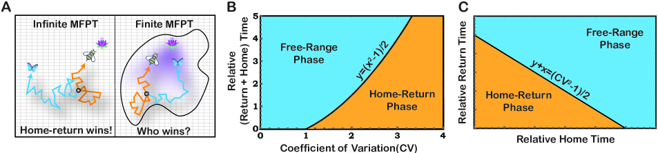
Figure 3: A. Search with home returns wins over free-range search whenever the mean FPT of the latter diverges. However, when the free-range mean FPT is finite, e.g., when the search arena is finite or when motion is biased in the direction of the target, either free-range search or search with home returns can have a lower mean FPT. B & C. The phase-space determined by Eq. (14) is spanned by three dimensionless parameters: the coefficient of variation of the free-range FPT, $CV=\sigma(T)/\langle T\rangle$, the relative mean return time, $\langle\tau(\vec{x})\rangle_{0}/\langle T\rangle$, and the relative mean home time $\langle W\rangle/\langle T\rangle$. When system parameters belong to the home-return (free-range) phase the introduction of home-returns is asserted to decrease (increase) the mean FPT to the target.

V A phase-diagram for search

The above example illustrates a situation where search with home returns offers significant performance advantage over free-range search. To generalize, one only needs to observe that since the mean FPT in Eq. (6) is finite for $r>0$ (under mild regularity conditions: $\langle W\rangle<\infty~{},\int_{\mathcal{D}}d\vec{x}~{}\tau(\vec{x})~{}G_{0}(\vec{x},t)<\infty$)—search with home returns offers a huge performance advantage in all conditions where the mean FPT of the underlying free-range process diverges (Fig. 3A left). This suggests that search with home returns performs best when search conditions are at their worst, but how to quantify and further extend this statement to situations where the underlying free-range FPT has a finite mean is not immediately clear as either free-range search or search with home returns may perform better (Fig. 3A right).

When does the introduction of home returns to a free-range search process lower the mean FPT to the target? To answer this question, one should take $\langle T_{r}\rangle$ in Eq. (6) and check when $d\langle T_{r}\rangle/dr|_{r=0}<0$, which we find happens when (Appendix K)

$$CV^{2}>1+\frac{2\langle\tau(\vec{x})\rangle_{0}}{\langle T\rangle}+\frac{2\langle W\rangle}{\langle T\rangle}~{}.$$ (14)

Here, $\langle T\rangle$ and $CV=\sigma(T)/\langle T\rangle$ are the mean and relative standard deviation (coefficient of variation) of the free-range FPT, $\langle W\rangle$ is the mean home-stay time, and $\langle\tau(\vec{x})\rangle_{0}=\int_{\mathcal{D}}~{}d\vec{x}~{}\tau(\vec{x})~{}\phi_{0}(\vec{x})=\frac{1}{\langle T\rangle}\int_{\mathcal{D}}~{}d\vec{x}~{}\tau(\vec{x})~{}\tilde{G}_{0}(\vec{x},0)$ is the mean return time in the limit $r\to 0$.

The condition in Eq. (14) relates three dimensionless quantities and reveals that search with home returns outperforms free-range search in conditions of high uncertainty. Indeed, on the left hand side of Eq. (14) stands the $CV$ which quantifies the relative magnitude of fluctuations, or uncertainty, around the free-range mean FPT. These fluctuations need to be large in order for the introduction of home-returns to be beneficial. On the right hand side of the inequality stand the relative mean return time, $\langle\tau(\vec{x})\rangle/\langle T\rangle$, and the relative mean home time, $\langle W\rangle/\langle T\rangle$, which act as penalties against home returns and set the bar for the critical magnitude of fluctuations at which the transition between the free-range phase and home-return phase occurs. The resulting phase-diagram for search is graphically illustrated in panels B & C of Fig. 3.

VI Drift-Diffusive search with home returns

To demonstrate how the universal result in Eq. (14) manifests itself in a concrete example, we consider a simple model for search in the presence of guidance cues. Namely, we consider the same diffusive search with home returns as in Fig. 2A above, but now assume that the particle also drifts at an average velocity $v$. Note that when the particle drifts away from the target ($v<0$) the free-range mean FPT diverges and search with home returns is always preferable (see discussion above). We thus focus on the $v>0$ case which could e.g., model search in the presence of an attractant (potential field) that biases the searcher’s motion in the direction of the target.

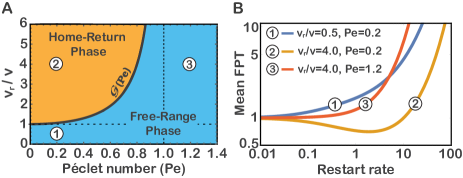
Figure 4: A. The phase space of drift-diffusive search as determined by Eq. (16). The free-range phase and home-return phase are separated by $\mathcal{G}(Pe)$ from Eq. (17). B. The mean FPT of drift-diffusive search with home returns vs. the restart rate (see Appendix M for details and corroboration via numerical simulations). Here, $L=v=1$, and other parameters are set by position in phase-space (numbered circles). When system parameters belong to the home return phase, e.g., for curve number (2), the introduction of home-returns decreases the mean FPT to the target. The converse happens for curves (1) & (3) whose parameters belong to the free-range phase.

The free-range propagator of drift-diffusion in the presence of an absorbing boundary (target) is known to be given by FPT1

$$G_{0}(x,t)=\frac{1}{\sqrt{4\pi Dt}}\left[e^{-\frac{(x-vt)^{2}}{4Dt}}-e^{\frac{Lv}{D}}e^{-\frac{(x-2L-vt)^{2}}{4Dt}}\right].$$ (15)

To build the search phase space, we first write all terms in Eq. (14) in terms of the natural parameters of drift-diffusion. Setting off from Eq. (15), a straightforward calculation gives $\langle T\rangle=L/v$ and $CV^{2}=1/Pe$, where $Pe=Lv/2D$ is the Péclet number FPT1 , i.e., the ratio between the rates of advective and diffusive transport. In addition, we find $\langle\tau(\vec{x})\rangle_{0}=\frac{L}{2v_{r}}\left(1-e^{-2Pe}-Pe+Pe^{2}\right)/Pe^{2}$, with $v_{r}$ standing once again for the home-return speed (Appendix L).

When $Pe\geq 1$ drift rules over diffusion which means that guidance cues towards the target are strong. Uncertainty in the free-range FPT is then relatively small and the condition in Eq. (14) cannot be satisfied since $CV^{2}=1/Pe\leq 1$. On the other hand, when $0<Pe<1$, diffusion rules over drift which means that guidance cues towards the target are weak. Uncertainty in the free-range FPT is then larger and we find that the condition in Eq. (14) is satisfied whenever (Appendix L, Fig. 4)

$$v_{r}>v\cdot\mathcal{G}(Pe)~{},$$ (16)

with

$$\mathcal{G}(Pe)=\frac{1-e^{-2Pe}}{Pe(1-Pe)}-1.$$ (17)

This means that the introduction of home returns will be beneficial whenever the return speed $v_{r}$ is greater than a critical speed $v_{r}^{*}=v\cdot\mathcal{G}(Pe)$. Measured in units of the drift velocity $v$, the critical return speed is uniquely determined by the Péclet number and hence by the relative uncertainty in the free-range FPT. When $Pe\ll 1$, $v_{r}^{*}\approx v$, but in the limit $Pe\to 1$, we have $v_{r}^{*}\sim v/(1-Pe)$. Thus, as guidance cues (drift) towards the target become stronger the return speed must increase sharply in order for search with home returns to remain beneficial.

VII Optimal search with home returns reduces mean and variance of time to target

When fluctuations in the free-range FPT are high such that the inequality in Eq. (14) holds, the introduction of home returns is asserted to lower the mean FPT to the target. This, in turn, implies the existence of an optimal restart rate $r^{*}>0$ for which the mean FPT, $\langle T_{r^{*}}\rangle$, is minimal. Reduction of the mean FPT is clearly important, but large fluctuations around the mean FPT can be deleterious as living organisms rely on a steady supply of nutrients and other essential resources. To this end, we now show that optimal search with home returns provides another important advantage: it reduces the variance of the FPT to the target.

Fluctuations around $\langle T_{r^{*}}\rangle$ have contributions coming from all stages of search, but note that those coming from the home stage are exclusively controlled by the searcher and can thus be made small. In fact, it is enough to require that $\sigma(W)\leq\langle W\rangle$ to show that the condition in Eq. (14) implies

$$\sigma(T_{r^{*}})^{2}\leq\langle T_{r^{*}}\rangle^{2}+2\langle T_{r^{*}}\rangle[\langle\tau(\vec{x})\rangle_{*}+\langle W\rangle]~{},$$ (18)

where the mean return time $\langle\tau(\vec{x})\rangle_{*}$ is computed like $\langle\tau(\vec{x})\rangle_{0}$ in Eq. (14), but with respect to the measure $\phi_{*}(\vec{x})=\tilde{G}_{*}(\vec{x},0)/\langle T_{r^{*}}\rangle$ such that

$$\langle\tau(\vec{x})\rangle_{*}=\frac{1}{\langle T_{r^{*}}\rangle}\int_{\mathcal{D}}d\vec{x}~{}\tau(x)\tilde{G}_{*}(\vec{x},0),$$ (19)

where $\tilde{G}_{*}(\vec{x},0)=\int_{0}^{\infty}~{}dt~{}G_{*}(\vec{x},t)$ and $G_{*}(\vec{x},t)$ is the propagator of the search process with home returns conducted at the optimal restart rate $r^{*}$.

Equation (18) is proven by contradiction. Assume this equation does not hold, and observe that this implies $\frac{\sigma(T_{r^{*}})^{2}}{\langle T_{r^{*}}\rangle^{2}}>1+\frac{2\langle\tau(\vec{x})\rangle_{*}}{\langle T_{r^{*}}\rangle}+\frac{2\langle W\rangle}{\langle T_{r^{*}}\rangle}~{}.$ Now, the condition in Eq. (14) asserts that the mean FPT time $\langle T_{r^{*}}\rangle$ can be lowered by restarting the entire search process at a small rate $\epsilon$. However, since the search stage is already being restarted at a rate $r^{*}$, the introduction of an additional restart rate $\epsilon$ amounts to restarting this stage at a rate $r^{*}+\epsilon$. Contrary to the search stage, the return and home stages are not restarted at a rate $r^{*}$. Thus, one only needs to consider what happens when both these stages are restarted at a rate $\epsilon$.

If the searcher is in the return stage it must have gotten there due to a restart event. Assuming that this restart event caught the searcher at some position $\vec{x}$, it will take the searcher $\tau(\vec{x})$ units of time to return home. In this return, the searcher will take a path that connects $\vec{x}$ with the origin (home). Consider a point $\vec{y}$ along this path, and let $\tau_{\vec{x}}(\vec{y})$ denote the remaining return time of a searcher which passes through $\vec{y}$ in his way back home from $\vec{x}$. In general, $\tau_{\vec{x}}(\vec{y})$ need not be equal to $\tau(\vec{y})$, i.e., to the time it takes the searcher to return from $\vec{y}$ when restart happens there. However, demanding that return times and paths obey $\tau_{\vec{x}}(\vec{y})=\tau(\vec{y})$ for every starting point $\vec{x}$ and every point $\vec{y}$ along a return path is very natural. Indeed, this only means that the time it takes the searcher to get back home from $\vec{y}$ does not depend on how it got there in the first place; and note that when this is the case restarting the return phase has no effect on the overall dynamics. Specifically, if a restart event catches the searcher during the return phase at a point $\vec{y}$ along a path connecting $\vec{x}$ with the origin, the searcher will take $\tau(\vec{y})$ units of time to return home from $\vec{y}$ which is exactly what would have happened in the absence of a restart event. We thus conclude that restarting the return phase at a rate $\epsilon$ has no effect, i.e., it is equivalent to not restarting the return phase at all.

Now, consider what happens when restart occurs during the home phase. Since $\tau(\vec{x}=\vec{0})=0$ by definition, the return time has zero contribution and one then only needs to understand the direct effect restart has on the duration of the time spent home. Recall that the home phase is on average $\langle W\rangle$ units of time long. Thus, if a restart event occurs during the home phase it will, on average, force the searcher to spend an additional $\langle W\rangle$ units of time at home. This time should be compared to the time the searcher would have spent home if restart would not have occurred at the moment it did. This time is known as the residual life time of $W$ Gallager , and renewal theory teaches us that its mean is given by $\langle W_{\text{res}}\rangle=\frac{\langle W^{2}\rangle}{2\langle W\rangle}=\frac{\sigma^{2}(W)+\langle W\rangle^{2}}{2\langle W\rangle}$. For example, if $W$ is deterministic, i.e., has zero variance, $\langle W_{\text{res}}\rangle=\langle W\rangle/2$ as restart would on average “catch” the searcher half way through its home stay duration. More generally, $\langle W_{\text{res}}\rangle$ can be smaller or larger than $\langle W\rangle$, but note that when $\sigma(W)<\langle W\rangle$ we always have $\langle W_{\text{res}}\rangle<\langle W\rangle$. Thus, when the standard deviation of the home stay time is smaller than its mean, restart will (on average) tend to prolong home stays as it “replaces” $\langle W_{\text{res}}\rangle$ with $\langle W\rangle$ which is longer.

From the above we conclude that if the addition of a small restart rate $\epsilon$ to all stages of search lowers the mean FPT below $\langle T_{r^{*}}\rangle$, then the addition of a small restart rate $\epsilon$ to the search phase only will also lower the mean FPT. Indeed, restarting the return phase is equivalent to not restarting it at all. In addition, not restarting the home phase (instead of restarting it at a rate $\epsilon$) will result in shorter home stays (provided that $\sigma(W)<\langle W\rangle$), which will lower the mean FPT even more as the target cannot be found while sitting at home. We thus find that $\langle T_{r^{*}+\epsilon}\rangle<\langle T_{r^{*}}\rangle$ which is, however, in contradiction to optimality as $r^{*}$ is defined to be the restart rate that brings $\langle T_{r}\rangle$ to a minimum. Concluding, we see that assuming that Eq. (18) does not hold leads to a contradiction, which means that this equation must hold.

From the above we draw an important conclusion. While there is no fundamental upper limit on fluctuations of free-range FPTs, those of optimal search with home returns must obey the bound in Eq. (18). Moreover, since $\langle T_{r^{*}}\rangle<\langle T\rangle$ by definition of the optimal restart rate $r^{*}$, we conclude that the combination of Eqs. (14) and (18) gives

$$\sigma(T_{r^{*}})<\sigma(T)~{},$$ (20)

whenever $\langle\tau(\vec{x})\rangle_{*}\leq\langle\tau(\vec{x})\rangle_{0}$. The latter condition is expected to hold in the generic case since a searcher that returns home from time to time will typically be found closer to home than one that does not. Thus, in addition to lowering the mean FPT to the target, optimal search with home returns also leads to a net reduction of fluctuations around the mean.

VIII Lévy search with home returns

To illustrate the double advantage conferred by search with home returns, we consider a Lévy walker that conducts search in a finite two-dimensional arena with multiple targets. Lévy walks Walks-CTRW1 ; Walks-CTRW2 ; Walks-CTRW3 ; Walks-CTRW4 ; Walks-CTRW5 have been widely applied to model animal foraging and motion HR3 ; Search1 ; Search2 ; Search3 ; Search4 ; Search6 ; Search7 as there are cases where they provide advantage over diffusive search strategies Search2 ; Search6 ; Search7 ; Search8 ; Walks-CTRW2 ; Levy-opt1 . It has thus been hypothesized that natural selection favours Lévy walks, which may explain their prevalence in nature. In what follows we show that the Lévy search strategy can be further improved when it is combined with home-returns. We start with a brief review of Lévy walks.

In the basic version of the Lévy walk model, a random walker travels along a straight line at a constant speed for some random time. At the end of the excursion, the walker randomly chooses a new direction of motion and travels along it (at the same speed) for another random duration before it turns again. The model is thus characterized by the travel speed $v_{LW}$ and the distribution of the random times between turning points. The latter are taken to be independent and identically distributed, and further assuming a finite mean and variance leads to motion that is asymptotically diffusive. However, when considering Lévy walks one is usually interested in cases where the long time asymptotics of the travel time probability density has a power-law form $\psi(\tau)\sim\tau^{-1-\alpha}$ with $0<\alpha<2$. This form leads to a diverging second moment and superdiffusive motion.

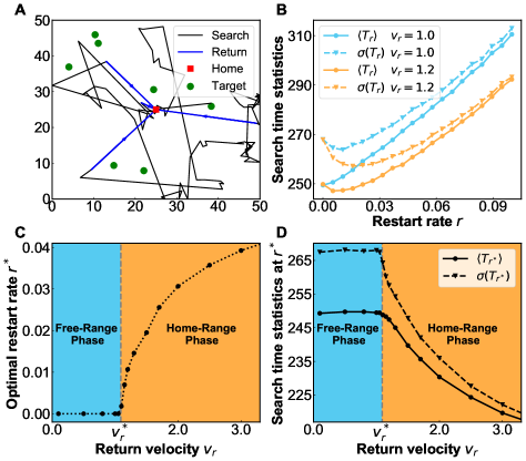
Figure 5: Optimal search with home returns reduces the mean and variance of the time to target. A. Here, this general feature is demonstrated for an agent foraging within a bounded two-dimensional arena. The agent performs a truncated Lévy walk with steps taken from a heavy-tailed distribution $\rho(l)\propto l^{-2}$. The search process is restarted at a rate $r$, and home returns are conducted at a constant speed $v_{r}$. The process ends when any one of the targets is found. B. The mean (circles) and standard deviation (triangles) of the first passage time vs. the restart rate for two different return speeds. C. The optimal restart rate for which the mean FPT $\langle T_{r}\rangle$ is minimized vs. the return speed. The critical return speed above which $r^{*}>0$ is estimated via Eq. (22). This method gives $v_{r}^{*}\simeq 1.09$ (dashed vertical line), which is in excellent agreement with independent numerical simulations of the home-return process for different values of $v_{r}$ (circles). D. The mean (circles) and standard deviation (triangles) of the first passage time under optimal restart vs. $v_{r}$. For $v_{r}>v_{r}^{*}$, both the mean and standard deviation of the FPT are strictly lower than those found for free-range search.

In Fig. 5A, we consider an agent whose task is to locate any one of seven targets that were placed randomly in a square arena. The agent conducts Lévy search with home returns. In the search phase, the agent performs a Lévy walk with $v_{LW}=1$. After each step the direction and length of the following step are chosen at random. The direction is drawn from the uniform angle distribution, whereas the step length is given by $l=v_{LW}\tau$, where $\tau=\tau_{0}/Z$ represents the random duration till the next turn. Taking $Z$ to be uniformly distributed on the unit interval $(0,1]$, one can show that $\psi(\tau)=\tau_{0}/\tau^{2}$ ($\tau>\tau_{0}$) which gives $\alpha=1$ Walks-CTRW6 . The probability density function governing the step length is then given by $\rho(l)=v_{LW}\tau_{0}/l^{2}$ for $l>v_{LW}\tau_{0}$, and we take $\tau_{0}=1$. Finally, in order to account for the finite size of the arena, we note that if the Lévy walker arrives at a boundary its step is truncated and a new step is generated. Thus, in practice, we consider a truncated Lévy walk Walks-CTRW2 .

The Lévy walk described above is restarted at a rate $r$, and home-returns are performed along the shortest possible path with a constant return speed $v_{r}$. To map the phase space of this search process, we scanned multiple $(v_{r},r)$ pairs. For each pair, we simulated $N=10^{6}$ sample trajectories that end when any one of the targets is hit during the search stage (recall that we assume that targets cannot be found during the return stage). In Fig. 5B, we plot the mean and standard deviation of the resulting FPT vs. the restart rate for two different values of the return speed $v_{r}=1$ and $v_{r}=1.2$. When $r=0$, search is conducted in the absence of home returns and we find that $\sigma(T)>\langle T\rangle$. Thus, in this example $CV>1$ and Eq. (14) asserts that the mean FPT can be lowered by the introduction of home-returns; provided the return speed is high enough (here we take $W=0$). Indeed, for $v_{r}=1.2$ we see that the mean FPT is minimized at $r^{*}>0$. However, the optimal restart rate for $v_{r}=1$ is $r^{*}=0$, which suggests that the critical return speed (above which home returns become beneficial) is somewhere in the range $1<v_{r}^{*}<1.2$.

The critical return speed $v_{r}^{*}$ can be determined via numerical evaluation of the mean return time $\langle\tau(\vec{x})\rangle_{0}$ in Eq. (14). To do this, we only need to simulate the search process without home returns ($r=0$). For each linear segment of the Lévy walk we note two quantities: the segment’s duration $\tau_{i}$, and the average distance of that segment to the home position (starting point), which we denote as $d_{i}$. Although such an average distance between a line segment and a point can in principle be calculated analytically, here we estimate its value by averaging over $10$ regularly spaced points along the segment (faster numerically). We then calculate the average return distance as

$$\overline{d}=\sum\limits_{i}d_{i}\tau_{i}/\sum\limits_{i}\tau_{i}~{}.$$ (21)

The mean return time in Eq. (14) is then given by $\langle\tau(\vec{x})\rangle_{0}=\overline{d}/v_{r}$, and substituting back into Eq. (14) gives $CV^{2}>1+\frac{2}{\langle T\rangle}\frac{\overline{d}}{v_{r}}.$ Rearranging, we find that the critical return speed is given by

$$v_{r}^{*}=\frac{2\overline{d}}{\sigma(T)^{2}/\langle T\rangle-\langle T\rangle},$$ (22)

which is uniquely determined by the free-range search process.

In Fig. 5C, we compare the estimate obtained from Eq. (22) to an independent estimate of $v_{r}^{*}$. The latter is obtained by direct numerical evaluation of the optimal restart rate. For a given return speed $v_{r}$, the optimal restart rate is found in two steps: (1) among the values of $r$ that were simulated we find the one that gives the shortest mean FPT, and then (2) we fit a quadratic function to the estimated mean FPT as a function of $r$ for six to eleven data points (adaptive algorithm) around the value found in (1). The quadratic function is used to predict the values of $r^{*}$ and $\langle T_{r^{*}}\rangle$. If the value of $r^{*}$ is predicted to be smaller than or equal to zero we take $r^{*}=0$ and the corresponding mean FPT as the optimal. The critical return velocity can then be determined as the smallest return velocity for which $r^{*}>0$. As can be seen, this method of estimating $v_{r}^{*}$ is in excellent agreement with the prediction coming from Eq. (22). Finally, for the optimal restart rates found, we plot the mean and standard deviation of the FPT vs. the return speed (Fig. 5D). For $v_{r}>v_{r}^{*}$, the mean and standard deviation are found to be lower than the values obtained in the absence of home-returns. Thus, optimal search with home returns reduces both the mean and variance of the time to target as predicted in the previous sections.

IX Conclusions and outlook

Search with home returns is widely observed in nature, but its analysis has so far been challenging. We developed a theoretical framework for this process and used it to show that solutions to first-passage problems with home-returns can always be given in terms of solutions to the corresponding free-range first-passage problems, i.e., those without home returns. The latter are known for a plethora of cases as first-passage time problems have been studied for decades; but even when this is not the case, the framework developed herein is still useful as it reduces a complicated problem to a much simpler one. Most importantly, our framework reveals a simple, and universal, phase-diagram for search. This, in turn, can be used to decide under which circumstances search with home returns is preferable to free-range search.

Our framework advances the field of first-passage under restart in several directions. First and foremost, it allows for a realistic description of restart by accounting for non-instantaneous and space-time coupled returns. To this end, the searcher’s return time was allowed to be an arbitrary function of its position at the restart moment, which naturally couples returns to the underlying stochastic motion. The latter can be general, which is also true for the distributions of restart and home-waiting times. Thus, our framework is applicable to a large variety of stochastic search processes, in arbitrary dimensions, and generally shaped domains that contain either single or multiple targets. Specifically, we provided general results for the mean [Eqs. (2) and (6)] and distribution [Eqs. (5) and (7)] of the first-passage time of a search process with home returns, and further demonstrated how these results apply to several case studies of interest.

To further elucidate the effect of home-returns, we asked under which conditions adopting this strategy is advantageous to search. We showed that this question can be answered based on the statistical properties of the underlying first-passage process, i.e., that which is conducted without home returns. This, in turn, gave us a phase diagram for search and revealed that search with home returns outperforms free-range search in conditions of high uncertainty. Specifically, the introduction of home returns will lower the mean FPT to a target whenever the relative magnitude of the fluctuations, or uncertainty, around the free-range mean FPT is large [Eq. (14)]. Moreover, under the same conditions, optimal search with home returns will also reduce the fluctuations around the mean FPT [Eq. (20)], which is important as living organisms rely heavily on a steady supply of nutrients and other essential resources. Indeed, even when the time taken to locate a resource is, on average, short enough to support life—large fluctuations around the average are deleterious and may result in death. Thus, search with home returns offers a double advantage, which unequivocally asserts the superiority of this strategy when facing uncertainty conditions.

While the prevalence of search with home returns in organisms ranging from insects to humans is probably due to the amalgamation of many contributing factors, our analysis shows that having a home may also be important as it allows one to locate food and other resources quickly and more efficiently than in its absence. Importantly, we find that this is true even when knowledge on the surrounding environment is not taken into account, and despite the fact that our analysis assumed that targets cannot be located in the return stage, i.e., while returning home. Thus, in reality, search with home returns is expected to perform even better than predicted here. Free-range search may out-compete search with home returns, but only in conditions of low uncertainty. This suggests that search with home returns may have evolved as a bet-hedging strategy that performs best when search conditions are at their worst.

Acknowledgments

The authors would like to acknowledge Tamás Kiss, Sergey Denisov and Eli Barkai, organizers of the 672. WE-Heraeus Seminar: “Search and Problem Solving by Random Walks”, as discussions that led to this work began there. Shlomi Reuveni would like to deeply acknowledge Sidney Redner for a series of joint discussions which led to this work. The authors would also like thank Guy Cohen and Ofek Lauber for commenting on early versions of this manuscript. Shlomi Reuveni acknowledges support from the Azrieli Foundation, from the Raymond and Beverly Sackler Center for Computational Molecular and Materials Science at Tel Aviv University, and from the Israel Science Foundation (grant No. 394/19). Arnab Pal acknowledges support from the Raymond and Beverly Sackler Post-Doctoral Scholarship at Tel-Aviv University.

Appendix A Detailed derivation of Eq. (2) in the main text

To derive Eq. (2) in the main text, we first rewrite Eq. (1) to obtain

$$T_{R}=\text{min}(T,R)+I(R\leq T)\left[\tau(\vec{x})+W+T_{R}^{\prime}\right]~{},$$ (23)

where $I(R\leq T)$ is an indicator function that takes the value one if $R\leq T$, and zero otherwise. Taking expectations on the both sides of the above equation, we obtain

$$\langle T_{R}\rangle=\langle\text{min}(T,R)\rangle+\langle I(R\leq T)\left[\tau(\vec{x})+W+T_{R}^{\prime}\right]\rangle.$$ (24)

Recalling that $W$ and $T_{R}^{\prime}$ are independent of $T$ and $R$, and that $\langle I(R\leq T)\rangle=\text{Pr}(R\leq T)$ by definition, we find

$$\langle T_{R}\rangle =\langle\text{min}(T,R)\rangle+\langle I(R\leq T)\tau(\vec{x})\rangle+\text{Pr}(R\leq T)\langle W\rangle$$

$$+\text{Pr}(R\leq T)\langle T_{R}^{\prime}\rangle.$$ (25)

Finally, as $T_{R}^{\prime}$ is an independent and identically distributed (IID) copy of $T_{R}$ we have $\langle T_{R}\rangle=\langle T_{R}^{\prime}\rangle$, and simple rearrangement then gives

$$\langle T_{R}\rangle=\frac{\langle\text{min}(T,R)\rangle}{\text{Pr}(T<R)}+\frac{\langle I(R\leq T)\tau(\vec{x})\rangle}{\text{Pr}(T<R)}+\frac{\text{Pr}(R\leq T)\langle W\rangle}{\text{Pr}(T<R)}.$$ (26)

Equation (26) is equivalent to Eq. (2) in the main text. Substituting Eq. (4) into Eq. (26), we observe that $\langle T_{R}\rangle$ can also be written as

$$\langle T_{R}\rangle = \frac{\langle\text{min}(T,R)\rangle}{\text{Pr}(T<R)}+\frac{\int_{0}^{\infty}~{}dt~{}f_{R}(t)\int_{\mathcal{D}}d\vec{x}~{}\tau(\vec{x})~{}G_{0}(\vec{x},t)}{\text{Pr}(T<R)}$$ (27)

$$+ \frac{\text{Pr}(R\leq T)\langle W\rangle}{\text{Pr}(T<R)}~{}.$$

Appendix B Evaluating terms in Eq. (2)

The expectation value, $\langle\text{min}(T,R)\rangle$, and the probability, $\text{Pr}(T<R)$, in Eq. (2) are easy to evaluate given the distributions of $T$ and $R$. Indeed, letting $f_{T}(t)$ and $f_{R}(t)$ stand for the probability densities of $T$ and $R$ respectively, we see that the cumulative distribution function of $\text{min}(T,R)$ is given by

$$\text{Pr}\left(\text{min}(T,R)\leq t\right)=1-\text{Pr}(T>t)\text{Pr}(R>t),$$ (28)

where

$$\text{Pr}(T>t)=\int_{t}^{\infty}~{}dt^{\prime}f_{T}(t^{\prime}),$$ (29)

and

$$\text{Pr}(R>t)=\int_{t}^{\infty}~{}dt^{\prime}f_{R}(t^{\prime}).$$ (30)

Now, since $\text{min}(T,R)$ is non-negative, the expectation $\langle\text{min}(T,R)\rangle$ can be computed directly from the cumulative distribution function in Eq. (28) as

$$\langle\text{min}(T,R)\rangle = \int_{0}^{\infty}~{}dt[1-\text{Pr}\left(\text{min}(T,R)\leq t\right)]$$ (31)

$$= \int_{0}^{\infty}~{}dt~{}\text{Pr}(T>t)\text{Pr}(R>t),$$

or, alternatively, using the density of $\text{min}(T,R)$ as

$$\langle\text{min}(T,R)\rangle = \int_{0}^{\infty}~{}dt~{}t[f_{T}(t)\text{Pr}(R>t)$$ (32)

$$+ f_{R}(t)\text{Pr}(T>t)].$$

Similarly, we see that the probability $\text{Pr}(T<R)$ is given by

$$\text{Pr}(T<R)=\int_{0}^{\infty}~{}dt~{}f_{R}(t)\text{Pr}(T<t)=\int_{0}^{\infty}~{}dt~{}f_{T}(t)\text{Pr}(R>t)~{},$$ (33)

and note that $\text{Pr}(R\leq T)=1-\text{Pr}(T<R)$.

Appendix C Detailed derivation of Eq. (5) in the main text

We will now derive an exact and general expression for the distribution of the FPT, $T_{R}$, in Laplace space. To this end, we first define two auxiliary random variables

$$R_{\text{min}} \equiv \{R|R\leq T\}~{},$$

$$T_{\text{min}} \equiv \{T|T<R\}~{}.$$ (34)

In words, $R_{\text{min}}$ is the restart time, $R$, conditioned on the event that restart occurs before the target is found. Similarly, $T_{\text{min}}$ is free-range FPT, $T$, conditioned on the event that the target is found prior to restart. The probability density functions of $R_{\text{min}}$ and $T_{\text{min}}$ are given by Restart-ND-5 ; Restart-D-3

$$f_{R_{\text{min}}}(t) = \frac{f_{R}(t)\int_{t}^{\infty}~{}dt^{\prime}~{}f_{T}(t^{\prime})}{\text{Pr}(R\leq T)}=\frac{f_{R}(t)\text{Pr}(T>t)}{\text{Pr}(R\leq T)}~{},$$

$$f_{T_{\text{min}}}(t) = \frac{f_{T}(t)\int_{t}^{\infty}~{}dt^{\prime}~{}f_{R}(t^{\prime})}{\text{Pr}(T<R)}=\frac{f_{T}(t)\text{Pr}(R>t)}{\text{Pr}(T<R)}~{}.$$ (35)

To obtain the Laplace transform of $T_{R}$, we utilize Eq. (1) and this gives

$$\tilde{T}_{R}(s) = \langle e^{-sT_{R}}\rangle$$

$$= \text{Pr}(T<R)~{}\left\langle e^{-sT_{R}}|T<R\right\rangle+\text{Pr}(R\leq T)~{}\left\langle e^{-sT_{R}}|R\leq T\right\rangle$$

$$= \text{Pr}(T<R)~{}\left\langle e^{-s\{T_{R}|T<R\}}\right\rangle+\text{Pr}(R\leq T)~{}\left\langle e^{-s\{T_{R}|R\leq T\}}\right\rangle.$$

However, by use of Eq. (1) and Eq. (34) above, we have

$$\{T_{R}|R\leq T\} = \{R+\tau(\vec{x})+W+T_{R}^{\prime}|R\leq T\}$$ (37)

$$= \{R+\tau(\vec{x})|R\leq T\}+W+T_{R}^{\prime}~{},$$

and

$$\{T_{R}|T<R\}=\{T|T<R\}=T_{\text{min}}~{},$$ (38)

where we have once again utilized the fact that $W$ and $T_{R}^{\prime}$ are independent of $R$ and $T$. Casting these relations back in Eq. (LABEL:SLT1), we obtain

$$\tilde{T}_{R}(s) = \text{Pr}(T<R)~{}\left\langle e^{-sT_{\text{min}}}\right\rangle+\text{Pr}(R\leq T)~{}\left\langle e^{-s(W+T_{R}^{\prime})-s\{R+\tau(\vec{x})|R\leq T\}}\right\rangle$$ (39)

$$= \text{Pr}(T<R)~{}\tilde{T}_{\text{min}}(s)+\text{Pr}(R\leq T)~{}\left\langle e^{-sW}\right\rangle~{}\left\langle e^{-sT_{R}^{\prime}}\right\rangle~{}\left\langle e^{-s\{R+\tau(\vec{x})|R\leq T\}}\right\rangle$$

$$= \text{Pr}(T<R)~{}\tilde{T}_{\text{min}}(s)+\text{Pr}(R\leq T)~{}\tilde{W}(s)~{}\tilde{T}_{R}(s)~{}\left\langle e^{-s\{R+\tau(\vec{x})|R\leq T\}}\right\rangle~{},$$

where we have again utilized the independence of $W$ and $T_{R}^{\prime}$, the fact that $T_{R}^{\prime}$ is an IID copy of $T_{R}$, and further used the shorthand notation $\tilde{Z}(s)$ to denote the Laplace transform of a random variable $Z$. We now observe that

$$\left\langle e^{-s\{R+\tau(\vec{x})|R\leq T\}}\right\rangle = \int_{0}^{\infty}~{}dt~{}f_{R_{\text{min}}}(t)~{}\left\langle e^{-s\{t+\tau(\vec{x}(t))|T\geq t\}}\right\rangle$$ (40)

$$= \int_{0}^{\infty}~{}dt~{}f_{R_{\text{min}}}(t)e^{-st}~{}\left[\frac{1}{\text{Pr}(T\geq t)}\int_{\mathcal{D}}~{}d\vec{x}~{}e^{-s\tau(\vec{x})}~{}G_{0}(\vec{x},t)\right]~{},$$

where we recall that $\text{Pr}(T\geq t)$ is the free-range survival probability. Substituting Eq. (35) into the above we obtain

$$\left\langle e^{-s\{R+\tau(\vec{x})|R\leq T\}}\right\rangle=\frac{1}{\text{Pr}(R\leq T)}\int_{0}^{\infty}~{}dt~{}f_{R}(t)e^{-st}~{}$$

$$\times\int_{\mathcal{D}}~{}d\vec{x}~{}e^{-s\tau(\vec{x})}~{}G_{0}(\vec{x},t)~{},$$ (41)

where we have used $\text{Pr}(T\geq t)=\text{Pr}(T>t)$. Equation (39) then reads

$$\tilde{T}_{R}(s)=\text{Pr}(T<R)~{}\tilde{T}_{\text{min}}(s)+\tilde{W}(s)~{}\tilde{T}_{R}(s)~{}\int_{0}^{\infty}~{}dt~{}f_{R}(t)e^{-st}$$

$$\times\int_{\mathcal{D}}d\vec{x}~{}e^{-s\tau(\vec{x})}~{}G_{0}(\vec{x},t).$$

Rearranging this expression, we obtain an exact and general expression for the FPT, $T_{R}$, in Laplace space

$$\tilde{T}_{R}(s)=\frac{\text{Pr}(T<R)\tilde{T}_{\text{min}}(s)}{1-\tilde{W}(s)\int_{0}^{\infty}~{}dt~{}f_{R}(t)e^{-st}~{}\int_{\mathcal{D}}~{}d\vec{x}~{}e^{-s\tau(\vec{x})}~{}G_{0}(\vec{x},t)}~{},$$

(43)

which is Eq. (5) as announced in the main text.

Appendix D Derivation of Eq. (6) in the main text

To derive Eq. (6) in the main text, we simplify Eq. (27) by assuming that $f_{R}(t)=re^{-rt}$, i.e., that restart times are taken from an exponential distribution with mean $1/r$. First, we use this in Eq. (31) to obtain

$$\langle\text{min}(T,R)\rangle = \int_{0}^{\infty}~{}dt~{}e^{-rt}\int_{t}^{\infty}~{}dt^{\prime}~{}f_{T}(t^{\prime})$$ (44)

$$= \frac{1}{r}-\frac{1}{r}\int_{0}^{\infty}dt~{}e^{-rt}f_{T}(t)$$

$$= \frac{1-\tilde{T}(r)}{r}~{},$$

where $\tilde{T}(r)$ stands for the Laplace transform of the free-range FPT, $T$, evaluated at $r$. Similarly, we use Eq. (33) to obtain

$$\text{Pr}(T<R)=\int_{0}^{\infty}~{}dt~{}f_{T}(t)e^{-rt}=\tilde{T}(r).$$ (45)

Finally, we see that for an exponentially distributed restart time we have

$$\int_{0}^{\infty}~{}dt~{}f_{R}(t)\int_{\mathcal{D}}d\vec{x}~{}\tau(\vec{x})~{}G_{0}(\vec{x},t)$$

$$=\int_{0}^{\infty}~{}dt~{}re^{-rt}\int_{\mathcal{D}}d\vec{x}~{}\tau(\vec{x})~{}G_{0}(\vec{x},t)$$

$$=r\int_{\mathcal{D}}d\vec{x}~{}\tau(\vec{x})~{}\int_{0}^{\infty}~{}dt~{}e^{-rt}G_{0}(\vec{x},t)$$

$$=r\int_{\mathcal{D}}d\vec{x}~{}\tau(\vec{x})~{}\tilde{G}_{0}(\vec{x},r),$$ (46)

where we have defined the Laplace transform of the free-range propagator as

$$\tilde{G}_{0}(\vec{x},r)=\int_{0}^{\infty}~{}dt~{}e^{-rt}~{}G_{0}(\vec{x},t)~{}.$$ (47)

Substituting Eqs. (44-46) into Eq. (27), we obtain

$$\langle T_{r}\rangle=\frac{1-\tilde{T}(r)}{\tilde{T}(r)}\frac{1}{r}+\frac{r\int_{\mathcal{D}}~{}d\vec{x}~{}\tau(\vec{x})~{}\tilde{G}_{0}(\vec{x},r)}{\tilde{T}(r)}+\frac{1-\tilde{T}(r)}{\tilde{T}(r)}\langle W\rangle~{}.$$

(48)

Finally, we observe that

$$\tilde{T}(r)=\int_{0}^{\infty}~{}dt~{}e^{-rt}~{}f_{T}(t) = -\int_{0}^{\infty}~{}dt~{}e^{-rt}~{}\frac{d\text{Pr}(T\geq t)}{dt}$$ (49)

$$= -\int_{0}^{\infty}~{}dt~{}e^{-rt}~{}\frac{d}{dt}\int_{\mathcal{D}}~{}d\vec{x}~{}G_{0}(\vec{x},t)$$

$$= 1-r\int_{\mathcal{D}}~{}d\vec{x}~{}\tilde{G}_{0}(\vec{x},r)~{},$$

where in the last transition we have used integration by parts and the definition in Eq. (47). Multiplying and dividing the second term on the right hand side of Eq. (48) by $1-\tilde{T}(r)$, using the relation in Eq. (49), and setting $\langle\tau(\vec{x})\rangle_{r}\equiv\int_{\mathcal{D}}~{}d\vec{x}~{}\tau(\vec{x})~{}\phi_{r}(\vec{x})\equiv\int_{\mathcal{D}}~{}d\vec{x}~{}\tau(\vec{x})~{}\tilde{G}_{0}(\vec{x},r)/\int_{\mathcal{D}}d\vec{x}~{}\tilde{G}_{0}(\vec{x},r)$, we obtain Eq. (6) in the main text.

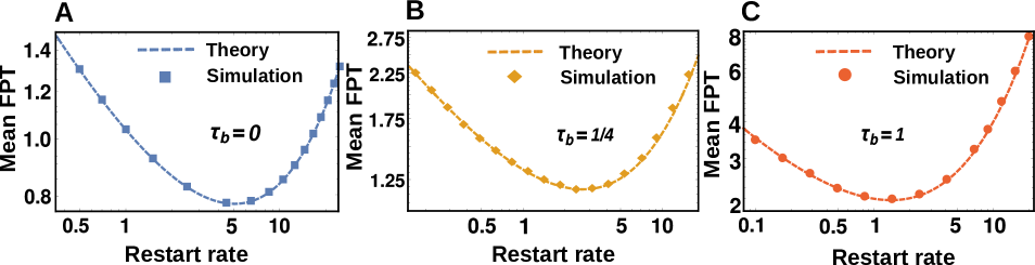
Figure 6: The Mean FPT of diffusive search with home returns is plotted vs. the restart rate $r$ for $\tau_{d}=1/2$ and three different values of $\tau_{b}$. Dashed lines come from Eq. (9) in the main text and markers indicate data coming from numerical simulations.

Appendix E Derivation of Eq. (7) in the main text

To derive Eq. (7) in the main text, we simplify Eq. (43) by assuming once again that $f_{R}(t)=re^{-rt}$, i.e., that restart times are taken from an exponential distribution with mean $1/r$. Using this in Eq. (35), we immediately find

$$\tilde{T}_{\text{min}}(s)=\int_{0}^{\infty}dt~{}e^{-st}~{}f_{T_{\text{min}}}(t) = \int_{0}^{\infty}dt~{}e^{-st}~{}\frac{f_{T}(t)\text{Pr}(R>t)}{\text{Pr}(T<R)}$$ (50)

$$= \frac{\tilde{T}(s+r)}{\tilde{T}(r)}~{},$$

where in the last step we have substituted Eq. (45) and used the fact that $\text{Pr}(R>t)=e^{-rt}$. Substituting $f_{R}(t)=re^{-rt}$, Eq. (45), and Eq. (50), into Eq. (43) and using the definition in Eq. (47), we recover Eq. (7) in the main text

$$\tilde{T}_{r}(s)=\frac{\tilde{T}(s+r)}{1-r~{}\tilde{W}(s)~{}\int_{\mathcal{D}}~{}d\vec{x}~{}e^{-s\tau(\vec{x})}\tilde{G}_{0}(\vec{x},s+r)}~{}.$$ (51)

Appendix F Derivation of Eq. (9) in the main text

To derive Eq. (9) in the main text, we simplify Eq. (6) for the case of diffusive home-range search. We first recall that in this case the free-range propagator (starting from the origin and in the presence of a target located at $L$) is given by FPT1

$$G_{0}(x,t)=\frac{1}{\sqrt{4\pi Dt}}\left(e^{-\frac{x^{2}}{4Dt}}-e^{-\frac{(2L-x)^{2}}{4Dt}}\right)~{}.$$ (52)

The Laplace transform of the propagator in Eq. (52) is given by

$$\tilde{G}_{0}(x,r) = \int_{0}^{\infty}dt~{}e^{-rt}G_{0}(x,t)$$ (53)

$$= \frac{1}{\sqrt{4Dr}}\left[e^{-\sqrt{\frac{r}{D}}|x|}-e^{-\sqrt{\frac{r}{D}}(2L-x)}\right]~{}.$$

Substituting the above expression into Eq. (49), we find

$$\tilde{T}(r) = 1-r\int_{\mathcal{D}}~{}d\vec{x}~{}\tilde{G}_{0}(\vec{x},r)$$ (54)

$$= 1-r\int_{-\infty}^{L}~{}dx~{}\tilde{G}_{0}(x,r)$$

$$= e^{-\sqrt{rL^{2}/D}}=e^{-\sqrt{\tau_{d}r}}~{},$$

where we recalled $\tau_{d}=L^{2}/D$ from Eq. (10). Finally, we observe that when the searcher returns home at a constant velocity $v_{r}$ we have $\tau(x)=|x|/v_{r}$, and this in turn results in

$$r\int_{\mathcal{D}}~{}d\vec{x}~{}\tau(\vec{x})~{}\tilde{G}_{0}(\vec{x},r) = r\int_{-\infty}^{L}~{}dx~{}\frac{|x|}{v_{r}}~{}\tilde{G}_{0}(x,r)$$

$$= \tau_{b}~{}e^{-\sqrt{\tau_{d}r}}\left[\frac{2\sinh(\sqrt{\tau_{d}r})}{\sqrt{\tau_{d}r}}-1\right]~{},$$

where we have recalled $\tau_{b}=L/v_{r}$ from Eq. (10) in the main text. Substituting Eqs. (54-LABEL:second-term) into Eq. (6) and setting $\langle W\rangle=0$, we recover Eq. (9) in the main text

$$\langle T_{r}\rangle=\frac{1}{r}\left(e^{\sqrt{\tau_{d}r}}-1\right)+\tau_{b}~{}\left[\frac{2\sinh(\sqrt{\tau_{d}r})}{\sqrt{\tau_{d}r}}-1\right]~{}.$$ (56)

Appendix G Corroboration of Eq. (9) in the main text via numerical simulations

In this section, we provide numerical corroboration of Eq. (9). In Fig. 6, we plot the mean FPT for $\tau_{d}=1/2$ and three different values of $\tau_{b}$ (indicated on plots) corresponding to those used in Fig. 2B in the main text. In all plots, dashed lines correspond to the exact analytical results coming from Eq. (9). These results are corroborated with data coming from numerical simulations (square, diamond, and circle markers). In the simulations, the time step was taken as $\Delta=10^{-5}$ and mean FPTs were estimated based on $10^{5}$ samples each. As seen from the figure, theory and simulations are in excellent agreement.

Appendix H Derivation of Eq. (11) in the main text

To derive Eq. (11), we start from Eq. (9) and set

$$\frac{d}{dr}\langle T_{r}\rangle=0~{},$$ (57)

which gives

$$2+2~{}\frac{\tau_{b}}{\tau_{d}}~{}z^{2}\cosh(z)+e^{z}(-2+z)=2~{}\frac{\tau_{b}}{\tau_{d}}~{}z\sinh(z),$$ (58)

with $z=\sqrt{r\tau_{d}}$. Substituting $2\cosh(z)=e^{z}+e^{-z}$ and $2\sinh(z)=e^{z}-e^{-z}$, we rewrite the above equation as

$$\frac{2}{z^{2}}\frac{1-e^{-z}-\frac{z}{2}}{(1-\frac{1}{z})+(1+\frac{1}{z})e^{-2z}}=\frac{\tau_{b}}{\tau_{d}}~{}.$$ (59)

The left-hand side of Eq. (59) was defined as $\mathcal{F}(z)$ in the main text.

Appendix I Expansion of $\mathcal{F}(z)$ around $z=0$

We recall the expression for $\mathcal{F}(z)$ from Eq. (9)

$$\mathcal{F}(z)=\frac{2}{z^{2}}\frac{1-e^{-z}-\frac{z}{2}}{(1-\frac{1}{z})+(1+\frac{1}{z})e^{-2z}}.$$ (60)

Expanding $\mathcal{F}(z)$ around $z=0$ gives

$$\mathcal{F}(z)=\frac{3}{2z^{3}}-\frac{2}{5z}-\frac{1}{8}+O(z)~{}.$$ (61)

Thus, in the limit $z\to 0$ we have $\mathcal{F}(z)=\frac{3}{2z^{3}}+O(\frac{1}{z})$.

Appendix J Derivation of Eq. (13) in the main text

To derive Eq. (13), we first write the MFPT from Eq. (9) at the optimal restart rate

$$\langle T_{r}\rangle\bigg{|}_{r=r^{*}}=\frac{1}{r^{*}}\left(e^{\sqrt{\tau_{d}r^{*}}}-1\right)+\tau_{b}~{}\left[\frac{2\sinh(\sqrt{\tau_{d}r^{*}})}{\sqrt{\tau_{d}r^{*}}}-1\right]~{}.$$ (62)

To capture the behavior of the MFPT at optimality, at the different limits, we first recall Eq. (12) from the main text

$$\begin{array}[]{l}r^{*}/r_{0}^{*}\simeq\left\{\begin{array}[]{lll}1&&\text{for ~{}~{}}\tau_{b}\ll\tau_{d}\text{ }\\ &\text{ \ \ }\\ \left(\frac{3}{2z_{0}^{*3}}\right)^{2/3}~{}\left(\frac{\tau_{b}}{\tau_{d}}\right)^{-2/3}&&\text{for~{}~{} }\tau_{b}\gg\tau_{d}\text{ ,}\end{array}\right.\text{ }\end{array}$$ (63)

where $r_{0}^{*}=z_{0}^{*2}/\tau_{d}$ and $z^{*}_{0}=1.593...$ is the solution of the transcendental equation $1-e^{-z}-\frac{z}{2}=0$. In the limit $\tau_{b}\ll\tau_{d}$, we have $r^{*}\simeq r_{0}^{*}$, and thus

$$\langle T_{r^{*}}\rangle\simeq\frac{e^{z_{0}^{*}}-1}{z_{0}^{*2}}\tau_{d}+\left[\frac{2\sinh(z_{0}^{*})}{z_{0}^{*}}-1\right]\tau_{b}\sim\tau_{d}~{}.$$ (64)

On the other hand, when $\tau_{b}\gg\tau_{d}$, we have $r^{*}/r_{0}^{*}\sim\left(\frac{\tau_{b}}{\tau_{d}}\right)^{-2/3}$, so $r^{*}\sim\tau_{d}^{-1/3}\tau_{b}^{-2/3}$, and $\tau_{d}r^{*}\sim\left(\frac{\tau_{b}}{\tau_{d}}\right)^{-2/3}\ll 1$. Substituting this scaling form into Eq. (62), we find

$$\langle T_{r^{*}}\rangle\simeq\frac{1}{r^{*}}\left(\sqrt{\tau_{d}r^{*}}+\frac{\tau_{d}r^{*}}{2}\right)+\tau_{b}\left(1+\frac{\tau_{d}r^{*}}{3}\right)\sim\tau_{b}.$$ (65)

Equation (13) then follows immediately from Eqs. (64-65).

Appendix K Derivation of Eq. (14) in the main text

To derive Eq. (14), we expand Eq. (48)

$$\langle T_{r}\rangle=\frac{1-\tilde{T}(r)}{r\tilde{T}(r)}+\frac{r\int_{\mathcal{D}}~{}d\vec{x}~{}\tau(\vec{x})~{}\tilde{G}_{0}(\vec{x},r)}{\tilde{T}(r)}+\frac{1-\tilde{T}(r)}{\tilde{T}(r)}\langle W\rangle,$$

around $r=0$ to obtain

$$\langle T_{r}\rangle=\langle T\rangle+\frac{r}{2}\left[\langle T\rangle^{2}-\sigma^{2}(T)\right] +r\int_{\mathcal{D}}~{}d\vec{x}~{}\tau(\vec{x})~{}\int_{0}^{\infty}~{}dt~{}G_{0}(\vec{x},t)$$

$$+r\langle T\rangle\langle W\rangle+\mathcal{O}(r^{2})~{},$$

with $\sigma^{2}(T)=\langle T^{2}\rangle-\langle T\rangle^{2}$ standing for the variance of $T$. Now, the introduction of home returns will decrease the FPT whenever $\langle T_{r}\rangle<\langle T\rangle$ which is equivalent to

$$\sigma^{2}(T)-\langle T\rangle^{2}>2\int_{\mathcal{D}}~{}d\vec{x}~{}\tau(\vec{x})~{}\int_{0}^{\infty}~{}dt~{}G_{0}(\vec{x},t)+2\langle T\rangle\langle W\rangle~{}.$$

Letting $CV=\sigma(T)/\langle T\rangle$ stand for the coefficient of variation, we rearrange the above expression and arrive at the following criterion

$$CV^{2}>1+\frac{2}{\langle T\rangle^{2}}\int_{\mathcal{D}}~{}d\vec{x}~{}\tau(\vec{x})\int_{0}^{\infty}~{}dt~{}G_{0}(\vec{x},t)+\frac{2\langle W\rangle}{\langle T\rangle}~{}.$$

(69)

To get Eq. (14), we rewrite the second term on the right hand side of Eq. (69) in a way that resembles the third term in this equation. Observe that

$$\frac{1}{\langle T\rangle}\int_{\mathcal{D}}~{}d\vec{x}~{}\tau(\vec{x})\int_{0}^{\infty}~{}dt~{}G_{0}(\vec{x},t)$$ (70)

$$= \int_{\mathcal{D}}~{}d\vec{x}~{}\tau(\vec{x})\left[\frac{1}{\langle T\rangle}\int_{0}^{\infty}~{}dt~{}G_{0}(\vec{x},t)\right]$$

$$= \int_{\mathcal{D}}~{}d\vec{x}~{}\tau(\vec{x})~{}\phi_{0}(\vec{x})~{},$$

where we have again used

$$\phi_{0}(\vec{x})=\phi_{r=0}(\vec{x}) = \tilde{G}_{0}(\vec{x},r=0)/\int_{\mathcal{D}}d\vec{x}~{}\tilde{G}_{0}(\vec{x},r=0)$$ (71)

$$= \frac{1}{\langle T\rangle}\int_{0}^{\infty}~{}dt~{}G_{0}(\vec{x},t)~{}.$$

Once again, we note that

$$\int_{\mathcal{D}}~{}d\vec{x}~{}\phi_{0}(\vec{x}) = \int_{\mathcal{D}}~{}d\vec{x}~{}\frac{1}{\langle T\rangle}\int_{0}^{\infty}~{}dt~{}G_{0}(\vec{x},t)$$ (72)

$$= \frac{1}{\langle T\rangle}\int_{0}^{\infty}~{}dt~{}\int_{\mathcal{D}}~{}d\vec{x}~{}G_{0}(\vec{x},t)$$

$$= \frac{1}{\langle T\rangle}\int_{0}^{\infty}~{}dt~{}\text{Pr}(T\geq t)$$

$$= 1,$$

which means that $\phi_{0}(\vec{x})$ is a proper probability density function over the domain $\mathcal{D}$. We thus have

$$\frac{1}{\langle T\rangle}\int_{\mathcal{D}}~{}d\vec{x}~{}\tau(\vec{x})\int_{0}^{\infty}~{}dt~{}G_{0}(\vec{x},t)=\int_{\mathcal{D}}~{}d\vec{x}~{}\tau(\vec{x})\phi(\vec{x})=\langle\tau(\vec{x})\rangle_{0}~{},$$

where the averaging over the return time is done with respect to the probability measure $\phi_{0}(\vec{x})$. Interpreting $\langle\tau(\vec{x})\rangle_{0}$ as the mean return time of a home-range searcher in the limit $r\to 0$, we substitute the above into Eq. (69) and recover Eq. (14) in the main text

$$CV^{2}>1+\frac{2\langle\tau(\vec{x})\rangle_{0}}{\langle T\rangle}+\frac{2\langle W\rangle}{\langle T\rangle}~{}.$$ (73)

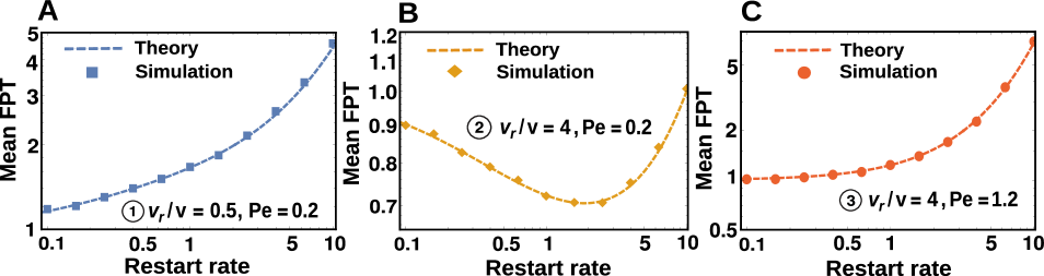
Figure 7: The mean FPT of drift-diffusive search with home returns is plotted vs. the restart rate $r$ for the three different sets of parameter that were used in Fig. 4B (indicated on plots). The dashed lines are exact theoretical results coming from Eq. (80) while the markers indicate data coming from numerical simulations.

Appendix L Drift-diffusive search with home returns

To derive an expression for the mean FPT of drift-diffusive search with home returns, we simplify Eq. (6) in the main text for this case. We start from the propagator of the free-range search process

$$G_{0}(x,t)=\frac{1}{\sqrt{4\pi Dt}}\left[e^{-\frac{(x-vt)^{2}}{4Dt}}-e^{\frac{Lv}{D}}e^{-\frac{(x-2L-vt)^{2}}{4Dt}}\right]~{},$$ (74)

and evaluate its Laplace transform (at $r$)

$$\tilde{G}_{0}(x,r) = \int_{0}^{\infty}~{}dt~{}e^{-rt}~{}G_{0}(x,t)$$

$$= \frac{e^{\frac{vx}{2D}}}{\sqrt{v^{2}+4Dr}}\left[e^{-\frac{|x|}{2D}\sqrt{v^{2}+4Dr}}-e^{-\frac{|x-2L|}{2D}\sqrt{v^{2}+4Dr}}\right].$$

Using the above expression, and Eq. (49), we compute the Laplace transform of the free-range first-passage time

$$\tilde{T}(r) = 1-r\int_{\mathcal{D}}~{}d\vec{x}~{}\tilde{G}_{0}(\vec{x},r)$$ (76)

$$= 1-r\int_{-\infty}^{L}~{}dx~{}\tilde{G}_{0}(x,r)$$

$$= e^{\frac{Lv}{2D}-\frac{L}{2D}\sqrt{v^{2}+4Dr}}.$$

To further proceed, we set $\tau(x)=|x|/v_{r}$ and compute

$$r\int_{\mathcal{D}}~{}d\vec{x}~{}\tau(\vec{x})~{}\tilde{G}_{0}(\vec{x},r) = r\int_{-\infty}^{L}~{}dx~{}\frac{|x|}{v_{r}}~{}\tilde{G}_{0}(x,r)$$ (77)

$$= \frac{e^{-\frac{L}{D}\sqrt{v^{2}+4Dr}}}{rv_{r}\sqrt{v^{2}+4Dr}}\bigg{[}2Dr\left(-1+e^{\frac{L}{D}\sqrt{v^{2}+4Dr}}\right)+v^{2}\left(e^{\frac{L}{D}\sqrt{v^{2}+4Dr}}-1\right)$$

$$+ v\sqrt{v^{2}+4Dr}-\left(v+rL\right)\sqrt{v^{2}+4Dr}~{}e^{\frac{L}{2D}\left(v+\sqrt{v^{2}+4Dr}\right)}\bigg{]}.$$

Using the above expression and Eq. (76), we find

$$\frac{r\int_{\mathcal{D}}~{}d\vec{x}~{}\tau(\vec{x})~{}\tilde{G}_{0}(\vec{x},r)}{\tilde{T}(r)} = \frac{r\int_{-\infty}^{L}~{}dx~{}\frac{|x|}{v_{r}}~{}\tilde{G}_{0}(x,r)}{\exp\bigg{[}\frac{Lv}{2D}-\frac{L}{2D}\sqrt{v^{2}+4Dr}\bigg{]}}$$ (78)

$$= \frac{e^{-\frac{Lv}{2D}-\frac{L}{2D}\sqrt{v^{2}+4Dr}}}{rv_{r}\sqrt{v^{2}+4Dr}}\bigg{[}2Dr\left(-1+e^{\frac{L}{D}\sqrt{v^{2}+4Dr}}\right)+v^{2}\left(e^{\frac{L}{D}\sqrt{v^{2}+4Dr}}-1\right)$$

$$+ \sqrt{v^{2}+4Dr}\left(v-\left(v+rL\right)~{}e^{\frac{L}{2D}\left(v+\sqrt{v^{2}+4Dr}\right)}\right)\bigg{]}.$$

Setting $\langle W\rangle=0$ and substituting Eq. (76) and Eq. (78) into Eq. (6), we find

$$\langle T_{r}\rangle = \frac{1}{r}\left[e^{\frac{L}{2D}\left(\sqrt{v^{2}+4Dr}-v\right)}-1\right]$$ (79)

$$+ \frac{e^{-\frac{Lv}{2D}}}{rv_{r}\sqrt{v^{2}+4Dr}}\bigg{[}(4Dr+2v^{2})\sinh\left(\frac{L}{2D}\sqrt{v^{2}+4Dr}\right)$$

$$+ \sqrt{v^{2}+4Dr}\left(ve^{-\frac{L}{2D}\sqrt{v^{2}+4Dr}}-v~{}e^{\frac{Lv}{2D}}-rL~{}e^{\frac{Lv}{2D}}\right)\bigg{]}.\hskip 18.49411pt$$

Recalling $Pe=Lv/2D$, $\tau_{d}=L^{2}/D$ and $\tau_{b}=L/v_{r}$, we can simplify the above expression further and obtain the following expression for the mean FPT of drift-diffusive search with home returns

$$\langle T_{r}\rangle=\frac{1}{r}\left[e^{\sqrt{Pe^{2}+\tau_{d}r}-Pe}-1\right]+\frac{1}{r}\frac{\tau_{b}}{\tau_{d}}~{}\mathcal{I}(Pe,\tau_{d},r)~{},$$ (80)

where we have introduced the following function

$$\mathcal{I}(Pe,\tau_{d},r) = 2e^{-Pe}\frac{2Pe^{2}+\tau_{d}r}{\sqrt{Pe^{2}+\tau_{d}r}}\sinh\left[\sqrt{Pe^{2}+\tau_{d}r}\right]$$ (81)

$$+ 2Pe\left[e^{-\left(Pe+\sqrt{Pe^{2}+\tau_{d}r}\right)}-1\right]-\tau_{d}r.$$

Eq. (80) and Eq. (81) together constitute a closed form expression for the mean FPT of drift-diffusive search with home returns.

Appendix M Corroboration of Eq. (80) via numerical simulations

In this section, we provide numerical corroboration of Eq. (80) for the mean FPT of drift-diffusive search with home returns. Equation (80) was used to plot Fig. 4B in the main text. In Fig. 7, we plot the mean FPT from Eq. (80) vs. the restart rate for three different sets of parameters (indicated on plots) which correspond to those used in Fig. 4B. In all the plots, dashed lines indicate analytical results coming from Eq. (80). These results are corroborated with data coming from numerical simulations (square, diamond, and circle markers). In the simulations, the time step was taken as $\Delta=10^{-5}$ and mean FPTs were estimated based on $10^{5}$ samples each. As seen from the figure, theory and simulations are in excellent agreement.

Appendix N Derivation of Eq. (16) in the main text

To derive Eq. (16), we simplify Eq. (14) in the main text for the case of drift-diffusive search with home returns. Starting from the propagator of the free-range search process

$$G_{0}(x,t)=\frac{1}{\sqrt{4\pi Dt}}\left[e^{-\frac{(x-vt)^{2}}{4Dt}}-e^{\frac{Lv}{D}}e^{-\frac{(x-2L-vt)^{2}}{4Dt}}\right],$$ (82)

the probability density function of the free-range first-passage time, $T$, can be computed by inverting Eq. (76) above. One then obtains FPT1

$$f_{T}(t)=\frac{L}{\sqrt{4\pi Dt^{3}}}e^{-\frac{(L-vt)^{2}}{4Dt}}.$$ (83)

The mean and coefficient of variation of $T$ are then easy to compute. These are given by

$$\langle T\rangle=L/v,$$ (84)

and

$$CV^{2}=2D/Lv=Pe^{-1},$$ (85)

where we recalled the definition of the Péclet number $Pe=Lv/2D$. With the above at hand, we continue to compute

$$\langle\tau(\vec{x})\rangle_{0}=\int_{\mathcal{D}}~{}d\vec{x}~{}\tau(\vec{x})~{}\phi(\vec{x}),$$ (86)

where $\phi(\vec{x})=\frac{1}{\langle T\rangle}\int_{0}^{\infty}~{}dt~{}G_{0}(\vec{x},t)$. First, we compute

$$\int_{0}^{\infty}~{}dt~{}G_{0}(x,t)=\frac{1}{v}~{}e^{\frac{vx}{2D}}\left[e^{-\frac{v|x|}{2D}}-e^{-\frac{v|x-2L|}{2D}}\right],$$ (87)

and this allows us to obtain

$$\int_{-\infty}^{L}~{}dx~{}\tau(x)~{}\int_{0}^{\infty}~{}dt~{}G_{0}(x,t)$$ (88)

$$= \int_{-\infty}^{L}~{}dx~{}\frac{|x|}{v_{r}}~{}\int_{0}^{\infty}~{}dt~{}G_{0}(x,t)$$

$$= \frac{1}{2v_{r}v^{3}}\left[4D^{2}(1-e^{-\frac{Lv}{D}})-2DLv+L^{2}v^{2}\right],$$

and conclude that

$$\langle\tau(\vec{x})\rangle_{0} = \frac{1}{2Lv_{r}v^{2}}\left[4D^{2}(1-e^{-\frac{Lv}{D}})-2DLv+L^{2}v^{2}\right]$$ (89)

$$= \frac{2D^{2}}{Lv_{r}v^{2}}\left[1-Pe+Pe^{2}-e^{-2Pe}\right].$$

Setting $\langle W\rangle=0$ and substituting the expressions for $\langle T\rangle$, $CV^{2}$, and $\langle\tau(\vec{x})\rangle_{0}$ into Eq. (14) we obtain

$$Pe^{-1}>1+\frac{v}{v_{r}}\frac{1-Pe+Pe^{2}-e^{-2Pe}}{Pe^{2}},$$ (90)

which can be rearranged to give Eq. (16) in the main text

$$v_{r}>v_{r}^{*}=v\cdot\mathcal{G}(Pe),~{}~{}\text{with~{}~{}}\mathcal{G}(Pe)=\frac{1-e^{-2Pe}}{Pe(1-Pe)}-1~{}.\hskip 18.49411pt$$ (91)

References

- (1) Song, C., Koren, T., Wang, P. and Barabási, A.L., 2010. Modelling the scaling properties of human mobility. Nature Physics, 6(10), p.818.
- (2) Simini, F., González, M.C., Maritan, A. and Barabási, A.L., 2012. A universal model for mobility and migration patterns. Nature, 484(7392), p.96.
- (3) Viswanathan, G.M., Da Luz, M.G., Raposo, E.P. and Stanley, H.E., 2011. The physics of foraging: an introduction to random searches and biological encounters. Cambridge University Press.
- (4) Darwin, C., 2004. On the origin of species, 1859. Routledge.
- (5) Viswanathan, G.M., Afanasyev, V., Buldyrev, S.V., Murphy, E.J., Prince, P.A. and Stanley, H.E., 1996. Lévy flight search patterns of wandering albatrosses. Nature, 381(6581), p.413.
- (6) Viswanathan, G.M., Buldyrev, S.V., Havlin, S., Da Luz, M.G.E., Raposo, E.P. and Stanley, H.E., 1999. Optimizing the success of random searches. nature, 401(6756), p.911.
- (7) Edwards, A.M., Phillips, R.A., Watkins, N.W., Freeman, M.P., Murphy, E.J., Afanasyev, V., Buldyrev, S.V., da Luz, M.G., Raposo, E.P., Stanley, H.E. and Viswanathan, G.M., 2007. Revisiting Lévy flight search patterns of wandering albatrosses, bumblebees and deer. Nature, 449(7165), p.1044.
- (8) Shlesinger, M.F., 2006. Mathematical physics: Search research. Nature, 443(7109), p.281.
- (9) Bénichou, O., Loverdo, C., Moreau, M. and Voituriez, R., 2011. Intermittent search strategies. Reviews of Modern Physics, 83(1), p.81.
- (10) Lomholt, M.A., Koren, T., Metzler, R. and Klafter, J., 2008. Lévy strategies in intermittent search processes are advantageous. Proceedings of the National Academy of Sciences, 105(32), pp.11055-11059.
- (11) Palyulin, V.V., Chechkin, A.V. and Metzler, R., 2014. Lévy flights do not always optimize random blind search for sparse targets. Proceedings of the National Academy of Sciences, 111(8), pp.2931-2936.
- (12) Levernier, N., Textor, J., Bénichou, O. and Voituriez, R., 2020. Inverse square Lévy walks are not optimal search strategies for d2. Physical Review Letters, 124(8), p.080601.
- (13) Redner, S., 2007. A Guide to First-Passage Processes. A Guide to First-Passage Processes, by Sidney Redner, Cambridge, UK: Cambridge University Press, 2007.
- (14) Bray, A.J., Majumdar, S.N. and Schehr, G., 2013. Persistence and first-passage properties in non-equilibrium systems. Advances in Physics, 62(3), pp.225-361.
- (15) Metzler, R., Redner, S. and Oshanin, G., 2014. First-Passage Phenomena and Their Applications (Vol. 35). Singapore: World Scientific.
- (16) Szabo, A., Schulten, K. and Schulten, Z., 1980. First passage time approach to diffusion controlled reactions. The Journal of chemical physics, 72(8), pp.4350-4357.
- (17) Schuss, Z., Singer, A. and Holcman, D., 2007. The narrow escape problem for diffusion in cellular microdomains. Proceedings of the National Academy of Sciences, 104(41), pp.16098-16103.
- (18) Condamin, S., Bénichou, O., Tejedor, V., Voituriez, R. and Klafter, J., 2007. First-passage times in complex scale-invariant media. Nature, 450(7166), pp.77-80.
- (19) Guérin, T., Levernier, N., Bénichou, O. and Voituriez, R., 2016. Mean first-passage times of non-Markovian random walkers in confinement. Nature, 534(7607), p.356.
- (20) Lanoiselée, Y., Moutal, N. and Grebenkov, D.S., 2018. Diffusion-limited reactions in dynamic heterogeneous media. Nature communications, 9(1), p.4398.
- (21) Evans, M.R., Majumdar, S.N. and Schehr, G., 2020. Stochastic resetting and applications. Journal of Physics A: Mathematical and Theoretical, 53(19), p.193001.
- (22) Evans, M.R. and Majumdar, S.N., 2011. Diffusion with stochastic resetting. Physical review letters, 106(16), p.160601.
- (23) Kusmierz, L., Majumdar, S.N., Sabhapandit, S. and Schehr, G., 2014. First order transition for the optimal search time of Lévy flights with resetting. Physical review letters, 113(22), p.220602.
- (24) Bhat, U., De Bacco, C. and Redner, S., 2016. Stochastic search with Poisson and deterministic resetting. Journal of Statistical Mechanics: Theory and Experiment, 2016(8), p.083401.
- (25) Pal, A., Kundu, A. and Evans, M.R., 2016. Diffusion under time-dependent resetting. Journal of Physics A: Mathematical and Theoretical, 49(22), p.225001.
- (26) Pal, A. and Reuveni, S., 2017. First Passage under Restart. Physical review letters, 118(3), p.030603.
- (27) Belan, S., 2018. Restart could optimize the probability of success in a Bernoulli trial. Physical review letters, 120(8), p.080601.
- (28) Chechkin, A. and Sokolov, I.M., 2018. Random search with resetting: a unified renewal approach. Physical review letters, 121(5), p.050601.
- (29) Pal, A., Eliazar, I. and Reuveni, S., 2019. First passage under restart with branching. Physical review letters, 122(2), p.020602.
- (30) Ray, S., Mondal, D. and Reuveni, S., 2019. Péclet number governs transition to acceleratory restart in drift-diffusion. Journal of Physics A: Mathematical and Theoretical, 52(25), p.255002.
- (31) Ray, S. and Reuveni, S., 2020. Diffusion with resetting in a logarithmic potential. J. Chem. Phys. 152, 234110.
- (32) Eliazar, I., Koren, T. and Klafter, J., 2007. Searching circular DNA strands. Journal of Physics: Condensed Matter, 19(6), p.065140.
- (33) Reuveni, S., Urbakh, M. and Klafter, J., 2014. Role of substrate unbinding in Michaelis-Menten enzymatic reactions. Proceedings of the National Academy of Sciences, 111(12), pp.4391-4396.
- (34) Rotbart, T., Reuveni, S. and Urbakh, M., 2015. Michaelis-Menten reaction scheme as a unified approach towards the optimal restart problem. Physical Review E, 92(6), p.060101.
- (35) Reuveni, S., 2016. Optimal stochastic restart renders fluctuations in first passage times universal. Physical review letters, 116(17), p.170601.
- (36) Robin, T., Reuveni, S. and Urbakh, M., 2018. Single-molecule theory of enzymatic inhibition. Nature communications, 9(1), p.779.
- (37) Evans, M.R. and Majumdar, S.N., 2018. Effects of refractory period on stochastic resetting. Journal of Physics A: Mathematical and Theoretical.
- (38) Pal, A. and Prasad, V.V., 2019. Landau-like expansion for phase transitions in stochastic resetting. Physical Review Research, 1(3), p.032001.
- (39) Masó-Puigdellosas, A., Campos, D. and Méndez, V., 2019. Stochastic movement subject to a reset-and-residence mechanism: transport properties and first arrival statistics. Journal of Statistical Mechanics: Theory and Experiment, 2019(3), p.033201.
- (40) Pal, A. and Prasad, V.V., 2019. First passage under stochastic resetting in an interval. Physical Review E, 99(3), p.032123.
- (41) Pal, A., Kusmierz, L. and Reuveni, S., 2019. Time-dependent density of diffusion with stochastic resetting is invariant to return speed. Physical Review E, 100(4), p.040101.
- (42) Pal, A., Kusmierz, L. and Reuveni, S., 2019. Invariants of motion with stochastic resetting and space-time coupled returns. New Journal of Physics, 21(11), p.113024.
- (43) Bodrova, A.S. and Sokolov, I.M., 2020. Resetting processes with noninstantaneous return. Physical Review E, 101(5), p.052130.
- (44) Maso-Puigdellosas, A., Campos, D. and Mendez, V., 2019. Transport properties of random walks under stochastic noninstantaneous resetting. Physical Review E, 100(4), p.042104.
- (45) Tal-Friedman, O., Pal, A., Sekhon, A., Reuveni, S. and Roichman, Y., 2020. Experimental realization of diffusion with stochastic resetting. arXiv preprint arXiv:2003.03096.
- (46) Montroll, E.W., 1969. Random Walks on Lattices. III. Calculation of First Passage Times with Application to Exciton Trapping on Photosynthetic Units. Journal of Mathematical Physics, 10(4), pp.753-765.
- (47) Kenkre, V.M., Montroll, E.W. and Shlesinger, M.F., 1973. Generalized master equations for continuous-time random walks. Journal of Statistical Physics, 9(1), pp.45-50.
- (48) Barkai, E., Metzler, R. and Klafter, J., 2000. From continuous time random walks to the fractional Fokker-Planck equation. Physical Review E, 61(1), p.132.
- (49) Bel, G. and Barkai, E., 2005. Weak ergodicity breaking in the continuous-time random walk. Physical Review Letters, 94(24), p.240602.
- (50) Klafter, J. and Sokolov, I.M., 2011. First steps in random walks: from tools to applications. Oxford University Press.
- (51) Shlesinger, M.F. and Klafter, J., 1986. Lévy walks versus Lévy flights. In On growth and form (pp. 279-283). Springer, Dordrecht.
- (52) Zaburdaev, V., Denisov, S. and Klafter, J., 2015. Lévy walks. Reviews of Modern Physics, 87(2), p.483.
- (53) Margolin, G. and Barkai, E., 2005. Nonergodicity of blinking nanocrystals and other Lévy-walk processes. Physical review letters, 94(8), p.080601.
- (54) Froemberg, D. and Barkai, E., 2013. Random time averaged diffusivities for Lévy walks. The European Physical Journal B, 86(7), p.331.
- (55) Dybiec, B., Gudowska-Nowak, E., Barkai, E. and Dubkov, A.A., 2017. Lévy flights versus Lévy walks in bounded domains. Physical Review E, 95(5), p.052102.
- (56) Kuśmierz, Ł. and Toyoizumi, T., 2017. Emergence of Lévy Walks from Second-Order Stochastic Optimization. Physical Review Letters, 119(25), p.250601.
- (57) Gallager, R.G., 2013. Stochastic processes: theory for applications. Cambridge University Press.
- (58) Bartumeus, F., Catalan, J., Fulco, U.L., Lyra, M.L. and Viswanathan, G.M., 2002. Optimizing the encounter rate in biological interactions: Lévy versus Brownian strategies. Physical Review Letters, 88(9), p.097901.