Parametric and non-parametric for extreme earthquake events
the joint tail inference for mainshocks and aftershocks

Parametric and non-parametric estimation of extreme earthquake event: the joint tail inference for mainshocks and aftershocks

Abstract

In an earthquake event, the combination of a strong mainshock and damaging aftershocks is often the cause of severe structural damages and/or high death tolls. The objective of this paper is to provide estimation for the probability of such extreme events where the mainshock and the largest aftershocks exceed certain thresholds. Two approaches are illustrated and compared – a parametric approach based on previously observed stochastic laws in earthquake data, and a non-parametric approach based on bivariate extreme value theory. We analyze the earthquake data from the North Anatolian Fault Zone (NAFZ) in Turkey during 1965–2018 and show that the two approaches provide unifying results.

Keywords and phrases: bivariate extreme value theory; earthquake data; tail probability; mainshock; aftershock
AMS 2010 Classification: 62G32 (60G70; 86A17).

1 Introduction

In a seismically active area, a strong earthquake, namely the mainshock, is often followed by subsequent damaging earthquakes, known as the aftershocks. These aftershocks may occur in numerous quantity and with magnitudes equivalent to powerful earthquakes on their own. For instance, in the 1999 İzmit earthquake, a magnitude 7.6 mainshock triggered hundreds of aftershocks with magnitudes greater than or equal to 4 in the first six days, cf. [25]. In the 2008 Sichuan earthquake, a mainshock of magnitude 8.0 induced a series of aftershocks with magnitudes up to 6.0. The results are severe structural damage and loss of life, especially when the area has already been weakened by the mainshock. The İzmit earthquake killed over 17,000 people and left half a million homeless [22]. The Sichuan earthquake caused over 69,000 deaths and damages of over 150 billion US dollars [9].

The goal of this paper is to provide a statistical analysis for the joint event of an extreme mainshock and extreme aftershocks. Throughout the paper, we denote the magnitude of a mainshock with $X$ and that of the largest aftershock with $Y$. We estimate via two approaches the probability of

$$\mathbb{P}(X>s,Y>t),$$ (1)

for large values of $s$ and $t$. The first approach uses a parametric model based on a series of well-know stochastic laws that describe the empirical relationships of the aftershocks and the mainshock, which we briefly review in Section 3.1. In the second approach, we apply bivariate extreme value theory to estimate the joint tail. Both methods are applied to the extreme earthquake events in the North Anatolian Fault Zone (NAFZ) in Turkey, the region where the 1999 İzmit earthquake occurred.

The remainder of the paper is structured as follows. In Section 2, we present the earthquake data in NAFZ and describe the relevant data processing. Section 3 provides the parametric and non-parametric estimation procedures for the joint main-/after-shock distribution. The detailed data analysis and results are presented in Section 4. We conclude in Section 5 with some discussions.

2 Data description

We use the North Anatolian Fault Zone (NAFZ) as an area of investigation due to its long and extensive historical record of large earthquakes [1; 2]. Extending from eastern Turkey to Greece, the 1,500-kilometer-long rip sustained several cycle-like sequences of large-magnitude ($M>7$) earthquakes over the past centuries [29], several resulting in high death tolls and severe economic losses. The most recent activities include the İzmit (Mw 7.6) and Düzce (Mw 7.1) earthquakes of 1999 [24; 28].

We obtain data from the Presidential of Earthquake Department database of the Turkish Disaster and Emergency Management Authority (https://deprem.afad.gov.tr/?lang=en) and consider all earthquake records between 1965–2018 with magnitudes 4 or higher in the area of $39.00^{o}-42.00^{o}$ latitude and $26.00^{o}-40.00^{o}$ longitude. The left panel of Figure 1 shows the time series of all earthquakes from 1965 onward.

We now label earthquake events by identifying the mainshocks and their corresponding aftershocks. Being interested in extreme events, we only consider earthquake events with significant mainshocks such that $X\geq 5$. We use the window algorithm proposed in [15] as follows. For each shock with magnitude $X\geq 5$, we scan the window within distance $L(X)$ and time $T(X)$. If a larger shock exists, we move on to that shock and perform the same scan. If not, then the shock is labelled as the mainshock and all shocks within the specified window are pronounced as its aftershocks. Table 1 provides the values for $L(X)$ and $T(X)$. For example, for an earthquake of magnitude 6.0, any shock following $T=510$ days and within $L=54$ km radius, with a magnitude less than 6, is considered to be its aftershock.

The right panel of Figure 1 shows the labelled mainshocks in the time series. The algorithm identifies $n=180$ earthquake events with mainshocks $X\geq 5$ among which 129 have aftershocks with magnitude greater than 4. Note that a few large earthquakes in the early years are not labelled as mainshocks, instead they are identified as aftershocks of mainshocks before the year 1965 from earlier data.

$X$	$L$	$T$
	(km)	(days)
5.0–5.4	40	155
5.5–5.9	47	290
6.0–6.4	54	510
6.5–6.9	61	790
7.0–7.4	70	915
7.5–7.9	81	960
8.0–8.4	94	985

Table 1: Window specification $L(X)$, $T(X)$ for aftershock labelling from [15].

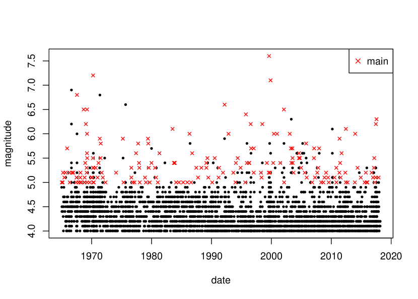
Figure 1: Shocks and labelled mainshocks in the NAFZ during 1965–2018.

3 Methodology

3.1 Parametric approach

It is agreed in the literature that the distribution of aftershocks in space, time and magnitude can be characterized by stochastic laws, see [30; 31] and [32] for a summary with detailed empirical studies. In this section, we propose a simple parametric model for the joint magnitudes of the mainshock and the largest aftershock based on these relationships. This derivation is similar to that in [33].

The following empirical evidence for aftershocks have been noted in prior literature.

1. The frequency $g(t)$ of the aftershocks per time unit at time $t$ after the mainshock follows the modified Omori’s law:

   $$g(t)=\frac{K}{(t+c)^{p}},$$

   where $K,c,p$ are constants [30].

2. The magnitude of the aftershocks follows Gutenberg-Richter’s law [16], that is, the number of aftershocks $N(m)$ with magnitude $m$ follows

   $$N(m)=10^{a-bm},$$ (2)

   where $a,b$ are constants.

3. The magnitude difference between a mainshock and its largest aftershock is approximately constant, independent of the mainshock magnitude and typically between 1.1 and 1.2 [3].

Based on the above, [30] modelled the intensity rate of aftershocks with magnitude $m$ as

$$\lambda(t,m)=\frac{10^{a+b(m_{0}-m)}}{(t+c)^{p}},\quad m\leq m_{0},$$ (3)

where $m_{0}$ is the mainshock magnitude and $a,b,c,p$ are constants. By defintion, $m\leq m_{0}$ such that aftershocks are always smaller than the mainshock. This modelling is used widely in ensuing literature, cf. [27], and is the basis of the ETAS (epidemic-type aftershock sequence) simulation model, cf. [23]. It is common to model the occurrences of aftershocks as a Poisson point process.

On the other hand, the mainshocks can be considered as independent events and their magnitude can also be modelled by the Gutenberg-Richter’s law in equation (2) [32]. In the following, we model the magnitude of the mainshocks $X$ using an exponential distribution with distribution and density functions

$$\mathbb{P}(X>x)=e^{-\alpha x},\quad f_{X}(x)=\alpha e^{-\alpha x}.$$ (4)

3.1.1 The model

Let $X_{A}$ denote the magnitude of an aftershock. Given the mainshock $X=m_{0}$, we assume that the aftershocks sequence follows a non-homogeneous Poisson process with intensity function (3). We derive the following.

• The total number of aftershocks $N$ follows a Poisson random variable with mean

  $$\mathbb{E}[N|X=m_{0}]=\sum_{t=1}^{\infty}\int_{0}^{m_{0}}\lambda(t,u)du=:Ce^{\beta m_{0}}\left(1-e^{-\beta m_{0}}\right),$$

  where $\beta=b\ln 10$ and $C=\frac{1}{\beta}10^{a}\sum_{t=1}^{\infty}\frac{1}{(t+c)^{p}}$.

• The conditional distribution of $X_{A}$ follows

  $$\mathbb{P}(X_{A}>m|X=m_{0})=\frac{\sum_{t=1}^{\infty}\int_{m}^{m_{0}}\lambda(t,u)du}{\sum_{t=1}^{\infty}\int_{0}^{m_{0}}\lambda(t,u)du}=\frac{e^{-\beta m}-e^{-\beta m_{0}}}{1-e^{-\beta m_{0}}},\quad 0\leq m\leq m_{0},$$

  and is conditionally independent of $N$.

Observe that the largest aftershock $Y=\max_{1\leq i\leq N}X_{A_{i}}$. Therefore, by the conditional independence of $N$ and $X_{A}$, it follows that for $m\in[0,m_{0}]$,

$$\mathbb{P}(Y\leq m|X=m_{0}) = \mathbb{E}\left[(1-P(X_{A}>m))^{N}|X=m_{0}\right]$$

$$= \exp\left\{-\mathbb{P}(X_{A}>m|X=m_{0}){\mathbb{E}[N|X=m_{0}]}\right\}$$

$$= \exp\left\{-\frac{e^{-\beta m}-e^{-\beta m_{0}}}{1-e^{-\beta m_{0}}}\cdot Ce^{\beta m_{0}}\left(1-e^{-\beta m_{0}}\right)\right\}$$

$$= \exp\left\{-C\left(e^{-\beta(m-m_{0})}-1\right)\right\},$$

where the second equality follows from a property of Poisson expectation: $\mathbb{E}[(1-p)^{N}]=\exp(-p\lambda)$, where $N\sim\text{Poi}(\lambda)$ and $p\in(0,1)$. Let $Z:=X-Y$, then $Z$ has distribution function

$$F(z):=P(Z\geq z)=\exp\left\{-C\left(e^{\beta z}-1\right)\right\},\quad z\leq m_{0}.$$ (5)

This suggests that $Z$ follows a Gompertz distribution, that is, $-Z$ follows a Gumbel distribution conditional to be negative. If we impose the convention that $\{Z>m_{0}\}=\{X_{A}<0\}$ represents the event that no aftershock occurs, then we can model $Z$ as independent of $X$. Note that when $m_{0}$ is large the probability of $\{Z>m_{0}\}$ is negligible.

Combining (4) and (5) yields the joint model for $(X,Y)$ given by

$$\mathbb{P}(X>x,Y>y)=\mathbb{P}(X>x,Z<X-y)=\int_{x}^{\infty}f_{X}(x)\int_{0}^{x-y}f_{Z}(z)dzdx,$$

where $f_{X}(x)$ is as defined in (4) and $f_{Z}(z)$ is the density function of $Z$ from (5). Given data, the parameters $(\alpha,\beta,C)$ can be estimated through maximum likelihood.

3.2 Bivariate extreme value approach

Multivariate extreme statistics has been exhibited to be a powerful tool for inference on multidimensional risk factors. Examples of applications can be found in [10; 21] and [26] among others. Recall that the goal is to estimate the probability: $\mathbb{P}(X>t,Y>s)$. To this end, we assume that the joint distribution of $(X,Y)$ is in the max domain of a bivariate extreme distribution introduced in [12]. This is a common condition in multivariate tail analysis and includes distributions with various types of copulas. Let $F_{1}$ and $F_{2}$ denote the marginal distribution functions of $X$ and $Y$, respectively. The assumption implies that for any $(x,y)\in[0,\infty]^{2}\setminus({\infty,\infty})$, the following limit exists:

$$\lim_{t\rightarrow 0}\frac{1}{t}\mathbb{P}(1-F_{1}(X)<tx,1-F_{2}(y)<ty)=:R(x,y).$$ (6)

The function $R$ characterizes the extremal dependence between $X$ and $Y$ and it can be expressed via other extremal dependence measures. For instance, it is linked to the stable tail dependence function $L$ and the Pickand function $A$:

$$R(x,y)=x+y-L(x,y)=(x+y)\left(1-A\left(\frac{y}{x+y}\right)\right).$$ (7)

For a general review on the multivariate extreme value theory, see for example Chapter 6 in [11] and Chapter 8 in [4].

The limit relation in (6) guarantees the regularity in the right tail of the copula of $(X,Y)$, which enables us to do the bivariate extrapolation to the range far beyond the historical observations. Let $s$ and $t$ be sufficiently large and denote that $p_{1}=\mathbb{P}(X>s)$ and $p_{2}=\mathbb{P}(X>t)$.

$$\mathbb{P}(X>s,Y>t) = \mathbb{P}(1-F_{1}(X)<p_{1},1-F_{2}(y)<p_{2})$$ (8)

$$= p_{2}\cdot\frac{1}{p_{2}}\mathbb{P}\left(1-F_{1}(X)<p_{2}\cdot\frac{p_{1}}{p_{2}},1-F_{2}(y)<p_{2}\right)$$

$$\approx p_{2}R\left(\frac{p_{1}}{p_{2}},1\right).$$

Then the problem transforms to estimating $p_{1}$, $p_{2}$ and $R(x,1)$. Due to the relation in (7), the various methods of estimating $L$ or $A$ can be applied to estimate $R(x,1)$; for instance see [8; 13; 7; 14; 5] among many others. Because of the particular features of earthquake data – that they have been rounded to the first digit and censored below – we use a basic non-parametric estimator of $R(x,1)$, which requires least assumptions on the data and is the basis of other more advanced estimation approaches. Let $n$ be the sample size and $k=k(n)$ be a sequence of integers such that $k\rightarrow\infty$ and $k/n\rightarrow 0$ as $n\rightarrow\infty$. Let $R_{i}^{X}$ and $R_{i}^{Y}$ denote the ranks of $X_{i}$ and $Y_{i}$ in their respective samples. The estimator of $R(x,1)$ is given by

$$\hat{R}(x,1)=\frac{1}{k}\sum_{i=1}^{n}I(R_{i}^{X}>n+1/2-kx,R_{i}^{Y}>n+1/2-k).$$ (9)

As for estimating $p_{1}$ and $p_{2}$, we fit exponential distributions to both margins, which is a typical choice for modeling earthquake magnitude justified by the Gutenberg–Richter law [16]. A natural alternative is to apply univariate extrem value theory to estimate these tail probabilities. Many studies have been devoted to study the tail distribution or the endpoint of earthquake magnitude; see for instance [19] and [6]. However, due to the small sample size and the rounding issue, we choose to fit parametric margins.

4 Results

From Section 2 we extract from the NAFZ dataset time series of mainshocks magnitude $(x_{i})$ where $x_{i}\geq 5$. For the time series of the corresponding largest aftershock, we only observe the values that are above 4, that is, we observe $\left(y_{i}\bf 1_{\{y_{i}\geq 4\}}\right)$. The two time series are plotted in Figure 2.

4.1 Parametric approach

The mainshock sequence $(x_{i})$ is fitted with an exponential distribution truncated at 4.95 – we take into consideration the continuity correction. Since all observations are discrete by 0.1 increment, from now on whenever we show the fit of a distribution or calculate the goodness-of-fit $p$-value, we jitter all observations by uniform noises between $(-.05,.05)$. The fit is shown on the left panel of Figure 3 and the Komogorov-Smirnov $p$-value is 0.83, indicating a good fit.

Next we fit a Gompertz distribution to the difference $x_{i}-y_{i}$ by maximizing the following censored likelihood:

$$L(\beta,C|x_{i},y_{i})=\prod_{y_{i}\geq 4}f_{Z}(x_{i}-y_{i};\beta,C)\prod_{y_{i}<4}(1-F_{Z}(x_{i}-4;\beta,C)),$$

where $F_{Z}$ is as defined in (5) and $f_{Z}$ is the corresponding density. To assess the goodness-of-fit, we first approximate the complete set of maximum aftershock sequence by $\tilde{y}_{i}$ as follows . When $y_{i}\geq 4$, set $\tilde{y}_{i}:=y_{i}$. When $y_{i}<4$, simulate $z_{i}$ from $F$ conditional on $z_{i}\geq x_{i}-4$ and set $\tilde{y}_{i}:=x_{i}-z_{i}$. The histogram of jittered $\tilde{y}_{i}$ is shown on the right panel of Figure 3 with the fitted density. The $p$-value is 0.95.

The scatterplot of the jittered $(x_{i},\tilde{y}_{i})$ is plotted in Figure 4, with the red point indicating the simulation for the censored observations. As we can see, the simulation is in agreement with the pattern of the observed pairs. We also note that the Båth’s law [3] – the empirical evidence that the magnitude difference between the mainshock and the largest aftershock is constant between 1.1 and 1.2 – can be well-justified by the fitted model. The fitted mean of $Y-X$ is 1.1. The $x=y+1.1$ line is shown in as the dotted line in Figure 4.

Figure 2: Time series of mainshocks (left) and largest aftershocks (right).

Figure 3: The histogram and fitted curve of: i) mainshocks with exponential distribution (left); ii) differences between mainshocks and largest aftershocks with Gompertz distribution (right).

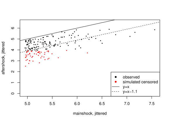
Figure 4: Scatterplot of mainshocks vs. aftershocks. Black indicates observations and red indicates censored aftershocks with magnitude $<4$ and simulated from the fitted model. The solid line indicate $y=x$. Clearly all observations falls below as $Y\leq X$ by definition. The dotted line indicates $y=x-1.1$ as suggested by the Båth’s law.

4.2 Extreme value approach

For the extreme value analysis approach, we use the same estimate for the marginal distribution of $X$ as in the parametric approach. We fit an exponential distribution truncated at 4.55 to the marginal distribution $Y$. The fitted density is shown in Figure 5 with the Komogorov-Smirnov $p$-value 0.11. The fitted distributions are used to compute $p_{1}$ and $p_{2}$ in (8).

When estimating $R(x,1)$, we note that there are ties in the data as they are rounded to one decimal place. For this, we randomly assign ranks to the tied observations. The missing values of $Y$ (they are censored above 4) does not effect the estimator in (9) provided that $k$ is smaller than $n_{1}$, the number of observed $Y_{i}$’s. Obviously, the ranks of the missing values are smaller than $n-n_{1}$, thus the corresponding indicator function in (9) equals to zero regardless of the precise value of $R_{i}^{Y}$.

The left panel of Figure 6 shows the estimates of $R(x,1)$ for three different values of $x$ and $k\in[10,100]$. Also note that $R(1,1)$ is a commonly used quantity to distinguish tail dependence ($R(1,1)>0$) and tail independence ($R(1,1)=0$). Roughly, tail dependence says that the extremes of X and Y tend to occur simultaneously while joint extremes rarely occur under tail independence. This plot clearly suggests tail dependence between $X$ and $Y$ because the estimates of $R(1,1)$ are clearly above zero. Based on these three curves, we choose our $k=40$.

With the choice of $k=40$, we obtain the non-parametric estimate of $R(x,1)$ for $x\in[0.02,5]$ plotted in the black curve in right panel of Figure 6. The wiggly behaviour of this estimator motivates us to consider a smoothing method. We adopt the smoothing method introduced in [20], which makes use of the beta copula. This smoothed estimator, denoted as $\hat{R}_{b}(x,1)$, respects the pointwise upper bounds of the function, that is $R(x,1)\leq\max(x,1)$ and it does not require smoothing parameter such as bandwidth. The resulted estimates are represented by the red curve in right panel of Figure 6. The two estimators are coherent with each other. $\hat{R}_{b}(x,1)$ is only used in obtaining the level curves in Figure 7.

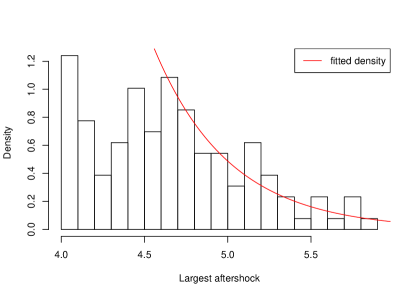
Figure 5: The histogram of the largest aftershocks and fitted exponential density

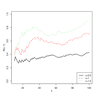
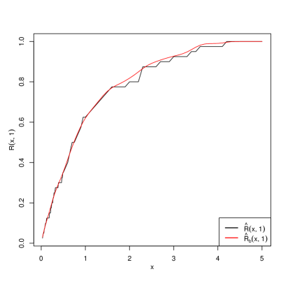
Figure 6: Left: The estimator of $R(x,1)$ is given in (9). Right: The estimator of $R(x,1)$ is given in (9).

4.3 Results and comparison

We are ready to estimate probabilities for the joint tail of $(X,Y)$. First, we estimate the tail probability defined in (8) for the ten largest earthquakes (mainshocks) in the NAFZ since 1965. As shown in the fifth and sixth column of Table 2, the estimates by two approaches are surprisingly close to each other, which supports the reasonability of the results. We emphasize that the two approaches only share one common assumption, that is, the marginal distribution of $X$. The distribution of $Y$ and the dependence between the $(X,Y)$ are modelled separately.

Next we obtain the level curves of $(X,Y)$ for the tail probability sequence

$$(10^{-3},5\cdot 10^{-4},10^{-4},5\cdot 10^{-5},10^{-5},5\cdot 10^{-6},10^{-6}),$$

as shown in Figure 7. The points $(x,y)$ on each curve represents such that $\mathbb{P}(X>x,Y>y)=p$ for the given probability level. Albeit based on different theories, the two approaches provide coinciding prediction results. The two dot lines in Figure  7 correspond to $x=y$ and $x=y+1.1$. The horizontal shape of the curves between these two lines indicates that the results respect the Båth’s law. This is particularly remarkable for the non-parametric approach, which does not impose any dependence structure for $(X,Y)$.

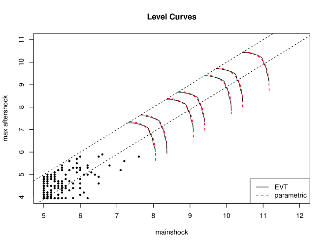
Figure 7: Predicted level curve for $(X,Y)$ based on the parametric model (red dotted) and extreme value analysis (black solid), with existing observations.

			largest	parametric	non-parametric
	date	mainshock	aftershock	probability	probability	location
1	1999-08-17	7.6	5.8	0.00265	0.00257	İzmit
2	1970-03-28	7.2	5.6	0.00618	0.00580	Gediz
3	1999-11-12	7.1	5.2	0.00815	0.00805	Düzce
4	1967-07-22	6.8	5.4	0.01413	0.01356	Mudurnu
5	1992-03-13	6.6	5.9	0.01429	0.01464	Erzincan
6	2002-02-03	6.5	5.8	0.01785	0.01827	Afyon
7	1969-03-28	6.5	4.9	0.02927	0.02745	Alaşehir
8	1968-09-03	6.5	4.6	0.03092	0.03051	Bartin
9	1995-10-01	6.4	5.0	0.03437	0.03296	Dinar
10	2017-07-20	6.3	5.1	0.03938	0.03747	Mugla Province

Table 2: Tail probability estimation for the ten largest earthquakes in the NAFZ since 1965.

5 Discussion

In this paper we consider estimating the tail probability of an extreme earthquake event where the mainshock magnitude $X$ and the largest aftershock magnitude $Y$ both exceed certain thresholds. We approach the problems from two directions. On one hand, based on the well-known stochastic rules for aftershocks, we propose a joint parametric model for $(X,Y)$, estimate the model using (censored) maximum likelihood, and from the model, calculate the desired probabilities. On the other hand, we use non-parametric methods from bivariate extreme value analysis to extrapolate tail probabilities. We illustrates both methods using the earthquake data in the North Anatolian Fault Zone (NAFZ) in Turkey from 1965 to 2018. The two approaches produce surprisingly agreeing results.

This is an exploratory effort in applying multivariate extreme value analysis to seismology problems and much extension is possible. For example, the occurrences of the earthquake events can be modelled in time and return level of extreme events can be estimated. Further information, such as distance between shocks and other geological covariates, can be incorporated into the analysis to provide more accurate or customized results.

This paper serves as a confirmation that simple techniques from multivariate extreme value analysis, though with little expert knowledge behind the data, is able to provide useful information in the analysis of extreme events.

References

- Ambraseys [1970] N. N. Ambraseys. Some characteristic features of the Anatolian fault zone. Tectonophysics, 9(2-3):143–165, 1970.
- Ambraseys and Finkel [1987] N.N. Ambraseys and C.F. Finkel. Seismicity of Turkey and neighbouring regions, 1899-1915. In Annales geophysicae. Series B. Terrestrial and planetary physics, volume 5, pages 701–725, 1987.
- Båth [1965] M. Båth. Lateral inhomogeneities of the upper mantle. Tectonophysics, 2(6):483–514, 1965.
- Beirlant et al. [2004] J. Beirlant, Y. Goegebeur, J. Segers, and J. Teugels. Statistics of Extremes, Theory and Applications. Chichester: Wiley, 2004.
- Beirlant et al. [2016] J. Beirlant, M. Escobar-Bach, Y. Goegebeur, and A. Guillou. Bias-corrected estimation of stable tail dependence function. Journal of Multivariate Analysis, 143:453–466, 2016.
- Beirlant et al. [2018] J. Beirlant, A. Kijko, T. Reynkens, and J.H.J. Einmahl. Estimating the maximum possible earthquake magnitude using extreme value methodology: the Groningen case. Natural Hazards, pages 1–23, 2018.
- Bücher et al. [2011] A. Bücher, H. Dette, and S. Volgushev. New estimators of the pickands dependence function and a test for extreme-value dependence. The Annals of Statistics, 39(4):1963–2006, 2011.
- Capéraà et al. [1997] P. Capéraà, A.-L. Fougères, and C. Genest. A nonparametric estimation procedure for bivariate extreme value copulas. Biometrika, 84(3):567–577, 1997.
- Cui et al. [2011] P. Cui, X.-Q. Chen, Y.-Y. Zhu, F.-H. Su, F.-Q. Wei, Y.-S. Han, H.-J. Liu, and J.-Q. Zhuang. The Wenchuan earthquake (May 12, 2008), Sichuan province, China, and resulting geohazards. Natural Hazards, 56(1):19–36, 2011.
- de Haan and de Ronde [1998] L. de Haan and J. de Ronde. Sea and wind: multivariate extremes at work. Extremes, 1(1):7, 1998.
- de Haan and Ferreira [2006] L. de Haan and A. Ferreira. Extreme Value Theory: An Introduction. Berlin: Springer, 2006.
- de Haan and Resnick [1977] L. de Haan and S. I. Resnick. Limit theory for multivariate sample extremes. Zeitschrift für Wahrscheinlichkeitstheorie und verwandte Gebiete, 40(4):317–337, 1977.
- Einmahl et al. [2008] J.H.J. Einmahl, A. Krajina, and J. Segers. A method of moments estimator of tail dependence. Bernoulli, 14(4):1003–1026, 2008.
- Fougères et al. [2015] A.-L. Fougères, L. De Haan, and C. Mercadier. Bias correction in multivariate extremes. The Annals of Statistics, 43(2):903–934, 2015.
- Gardner and Knopoff [1974] J.K. Gardner and L. Knopoff. Is the sequence of earthquakes in Southern California, with aftershocks removed, Poissonian? Bulletin of the Seismological Society of America, 64(5):1363–1367, 1974.
- Gutenberg and Richter [1944] B. Gutenberg and C. F. Richter. Frequency of earthquakes in California. Bulletin of the Seismological Society of America, 34(4):185–188, 1944.
- Hanks and Kanamori [1979] T. C. Hanks and H. Kanamori. A moment magnitude scale. Journal of Geophysical Research: Solid Earth, 84(B5):2348–2350, 1979.
- Kanamori [1977] H. Kanamori. The energy release in great earthquakes. Journal of geophysical research, 82(20):2981–2987, 1977.
- Kijko [2004] A. Kijko. Estimation of the maximum earthquake magnitude, m max. Pure and Applied Geophysics, 161(8):1655–1681, 2004.
- Kiriliouk et al. [2018] A. Kiriliouk, J. Segers, and L. Tafakori. An estimator of the stable tail dependence function based on the empirical beta copula. Extremes, 21(4):581–600, 2018.
- Ledford and Tawn [1997] A. W. Ledford and J. A. Tawn. Modelling dependence within joint tail regions. Journal of the Royal Statistical Society: Series B (Statistical Methodology), 59(2):475–499, 1997.
- Marza [2004] V.I. Marza. On the death toll of the 1999 Izmit (Turkey) major earthquake. ESC General Assembly Papers, European Seismological Commission, Potsdam, 2004.
- Ogata [1988] Y. Ogata. Statistical models for earthquake occurrences and residual analysis for point processes. Journal of the American Statistical association, 83(401):9–27, 1988.
- Parsons et al. [2000] T. Parsons, S. Toda, R. S. Stein, A. Barka, and J. H Dieterich. Heightened odds of large earthquakes near istanbul: An interaction-based probability calculation. Science, 288(5466):661–665, 2000.
- Polat et al. [2002] O. Polat, H. Eyidogan, H. Haessler, A. Cisternas, and H. Philip. Analysis and interpretation of the aftershock sequence of the August 17, 1999, Izmit (Turkey) earthquake. Journal of Seismology, 6(3):287–306, 2002.
- Poon et al. [2004] S.-H. Poon, M. Rockinger, and J. Tawn. Extreme-value dependence in financial markets: diagnostics, models and financial implications. Review of Financial Studies, 17:581 – 610, 2004.
- Reasenberg and Jones [1989] P. A Reasenberg and L. M. Jones. Earthquake hazard after a mainshock in California. Science, 243(4895):1173–1176, 1989.
- Reilinger et al. [2000] R.E. Reilinger, S. Ergintav, R. Bürgmann, S. McClusky, O. Lenk, A. Barka, O. Gurkan, L. Hearn, K.L. Feigl, and R. Cakmak. Coseismic and postseismic fault slip for the 17 August 1999, M= 7.5, Izmit, Turkey earthquake. Science, 289(5484):1519–1524, 2000.
- Stein et al. [1997] R. S. Stein, A. A Barka, and J. H. Dieterich. Progressive failure on the North Anatolian fault since 1939 by earthquake stress triggering. Geophysical Journal International, 128(3):594–604, 1997.
- Utsu [1970] T. Utsu. Aftershocks and earthquake statistics (1): Some parameters which characterize an aftershock sequence and their interrelations. Journal of the Faculty of Science, Hokkaido University. Series 7, Geophysics, 3(3):129–195, 1970.
- Utsu [1971] T. Utsu. Aftershocks and earthquake statistics (2): Further investigation of aftershocks and other earthquake sequences based on a new classification of earthquake sequences. Journal of the Faculty of Science, Hokkaido University. Series 7, Geophysics, 3(4):197–266, 1971.
- Utsu [1972] T. Utsu. Aftershocks and earthquake statistics (3): Analyses of the distribution of earthquakes in magnitude, time and space with special consideration to clustering characteristics of earthquake occurrence (1). Journal of the Faculty of Science, Hokkaido University. Series 7, Geophysics, 3(5):379–441, 1972.
- Vere-Jones et al. [2006] D. Vere-Jones, J. Murakami, and A. Christophersen. A further note on Bath’s law. In The 4th International Workshop on Statistical Seismology (Statsei4), pages 611–0011, 2006.