Finding optimal solutions by stochastic cellular automata

Abstract

Finding a ground state of a given Hamiltonian is an important but hard problem. One of the potential methods is to use a Markov chain Monte Carlo (MCMC) to sample the Gibbs distribution whose highest peaks correspond to the ground states. In this short paper, we use stochastic cellular automata (SCA) and see if it is possible to find a ground state faster than the conventional MCMCs, such as the Glauber dynamics. We show that, if the temperature is sufficiently high, it is possible for SCA to have more spin-flips per update in average than Glauber and, at the same time, to have an equilibrium distribution “close” to the one for Glauber, i.e., the Gibbs distribution. During the course, we also propose a new way to characterize how close a probability measure is to the target Gibbs.

1 Introduction

There are many occasions in real life when we have to quickly choose one among extremely many options. In addition, we want our choice to be optimal in a certain sense. Such optimization problems are ubiquitous and possibly quite hard to solve them fast. In particular, NP-hard problems cannot be solved in polynomial time [3].

One approach to find an optimal solution to a given problem is to translate it into an Ising model (see, e.g., [8] for a list of examples of such mappings) and find its ground state that corresponds to an optimal solution. A standard method to do so is to use a Markov chain Monte Carlo (MCMC) to sample the Gibbs distribution $\pi^{\scriptscriptstyle\rm G}_{\beta}(\boldsymbol{\sigma})\propto e^{-\beta H(\boldsymbol{\sigma})}$, where $\beta\geq 0$ is the inverse temperature and $H(\boldsymbol{\sigma})$ is the corresponding Ising Hamiltonian. The ground states are the spin configurations at which the Gibbs distribution takes on its highest peaks.

There are several MCMCs that generate the Gibbs distribution. In most of the popular ones, such as the Glauber dynamics [5], the number of spin-flips per update is at most one, which makes them inefficient. We have longed for faster MCMCs.

We consider probabilistic cellular automata, or PCA for short [2, 11]. Since the term PCA has already been used for long as an abbreviation for principal component analysis in statistics, we should rather call it stochastic cellular automata (SCA). It is an MCMC based on independent multi-spin flip dynamics, and therefore it is potentially faster than the standard single-spin flip MCMCs.

However, since the SCA equilibrium $\pi^{\scriptscriptstyle\rm SCA}_{\beta,q}$ is different from $\pi^{\scriptscriptstyle\rm G}_{\beta}$, we cannot naively use it as a Gibbs sampler to search for the ground states. Only when the pinning parameter $q\geq 0$ goes to infinity, the total variation distance $\|\pi^{\scriptscriptstyle\rm SCA}_{\beta,q}-\pi^{\scriptscriptstyle\rm G}_{\beta}\|_{\scriptscriptstyle\text{TV}}$ goes to zero. The downside of this limit is the slowdown effect on SCA: each spin is more likely to stick to the current state for larger values of $q$ (this is why we call it the pinning parameter).

In this paper, we investigate SCA and try to find by simple arithmetic an interval of $q$ that is compatible with good approximation to Gibbs and, at the same time, faster than Glauber. In Section 2, we define relevant observables, such as the Hamiltonian, the transition probabilities for Glauber and SCA, and their equilibrium distributions. In Section 3, we show an upper bound on $q$ below which SCA is faster than Glauber in terms of the expected number of spin-flips per update, not in terms of the mixing time. In Section 4, we show a lower bound on $q$ above which the SCA equilibrium $\pi^{\scriptscriptstyle\rm SCA}_{\beta,q}$ is close to the target Gibbs $\pi^{\scriptscriptstyle\rm G}_{\beta}$ in the sense of order-preservation (see (4.2) for the precise definition), rather than in the total variation distance. Thanks to this new notion of closeness, it becomes tractable to obtain a quantitative estimate on the difference between the two equilibrium measures. This is crucial especially when we apply the theory to real-life situations or numerical simulations. In the last section, Section 5, we give a conclusion obtained from the results in Sections 3–4, which can be stated in short words as follows.

Theorem 1.1.

If $\beta$ is sufficiently small, then we can define SCA for which the following both hold at the same time:

• SCA is faster than Glauber in terms of the expected number of spin-flips per update.

• If the SCA equilibrium $\pi^{\scriptscriptstyle\rm SCA}_{\beta,q}$ takes on its highest peak at $\boldsymbol{\sigma}$, then $\boldsymbol{\sigma}$ is close to the ground states of $H$ up to a certain error (see Theorem 5.1 for the precise statement).

At the end of this paper, we also discuss implications of the above theorem and an idea to find the ground states without using any cooling methods.

2 Definition

Given a finite graph $G=(V,E)$ with no multi- or self-edges, spin-spin couplings $\{J_{x,y}\}_{\{x,y\}\in E}$ (with $J_{x,y}=0$ if $\{x,y\}\notin E$) and local magnetic fields $\{h_{x}\}_{x\in V}$, we define the Hamiltonian for the spin configuration $\boldsymbol{\sigma}=\{\sigma_{x}\}_{x\in V}\in\{\pm 1\}^{V}$ as

$$H(\boldsymbol{\sigma})=-\sum_{\{x,y\}\in E}J_{x,y}\sigma_{x}\sigma_{y}-\sum_{x\in V}h_{x}\sigma_{x}=-\frac{1}{2}\sum_{x,y\in V}J_{x,y}\sigma_{x}\sigma_{y}-\sum_{x\in V}h_{x}\sigma_{x}.$$ (2.1)

Let $w^{\scriptscriptstyle\rm G}_{\beta}$ and $\pi^{\scriptscriptstyle\rm G}_{\beta}$ be the Boltzmann weight and the Gibbs distribution, respectively, at the inverse temperature $\beta\geq 0$:

$$w^{\scriptscriptstyle\rm G}_{\beta}(\boldsymbol{\sigma})=e^{-\beta H(\boldsymbol{\sigma})}, \pi^{\scriptscriptstyle\rm G}_{\beta}(\boldsymbol{\sigma})=\frac{w^{\scriptscriptstyle\rm G}_{\beta}(\boldsymbol{\sigma})}{\sum_{\boldsymbol{\sigma}}w^{\scriptscriptstyle\rm G}_{\beta}(\boldsymbol{\sigma})}.$$ (2.2)

For $\boldsymbol{\sigma}\in\{\pm 1\}$, $I\subset V$ and $x\in V$, we let

$$(\boldsymbol{\sigma}^{I})_{y}=\begin{cases}\sigma_{y}&[y\notin I],\\ -\sigma_{y}\quad&[y\in I],\end{cases} \boldsymbol{\sigma}^{x}=\boldsymbol{\sigma}^{\{x\}}.$$ (2.3)

It is known that $\pi^{\scriptscriptstyle\rm G}_{\beta}$ is the equilibrium distribution for the Glauber dynamics whose transition probability is defined as

$$P^{\scriptscriptstyle\rm G}_{\beta}(\boldsymbol{\sigma},\boldsymbol{\tau})=\begin{cases}\displaystyle\frac{1}{|V|}\frac{w^{\scriptscriptstyle\rm G}_{\beta}(\boldsymbol{\sigma}^{x})}{w^{\scriptscriptstyle\rm G}_{\beta}(\boldsymbol{\sigma})+w^{\scriptscriptstyle\rm G}_{\beta}(\boldsymbol{\sigma}^{x})}\quad&[\boldsymbol{\tau}=\boldsymbol{\sigma}^{x}],\\[12.0pt] \displaystyle 1-\sum_{x\in V}P^{\scriptscriptstyle\rm G}_{\beta}(\boldsymbol{\sigma},\boldsymbol{\sigma}^{x})&[\boldsymbol{\tau}=\boldsymbol{\sigma}],\\ 0&[\text{otherwise}].\end{cases}$$ (2.4)

By introducing the cavity fields $\tilde{h}_{x}(\boldsymbol{\sigma})$, defined as

$$\tilde{h}_{x}(\boldsymbol{\sigma})=\sum_{y\in V}J_{x,y}\sigma_{y}+h_{x},$$ (2.5)

the Glauber transition probability $P^{\scriptscriptstyle\rm G}_{\beta}(\boldsymbol{\sigma},\boldsymbol{\sigma}^{x})$ can be written as

$$P^{\scriptscriptstyle\rm G}_{\beta}(\boldsymbol{\sigma},\boldsymbol{\sigma}^{x})=\frac{1}{|V|}\frac{e^{-\beta\tilde{h}_{x}(\boldsymbol{\sigma})\sigma_{x}}}{2\cosh(\beta\tilde{h}_{x}(\boldsymbol{\sigma}))}.$$ (2.6)

Next we define SCA. First we let

$$\tilde{H}(\boldsymbol{\sigma},\boldsymbol{\tau})=-\frac{1}{2}\sum_{x,y\in V}J_{x,y}\sigma_{x}\tau_{y}-\frac{1}{2}\sum_{x\in V}h_{x}(\sigma_{x}+\tau_{x}).$$ (2.7)

Notice that

$$\tilde{H}(\boldsymbol{\sigma},\boldsymbol{\tau})=\tilde{H}(\boldsymbol{\tau},\boldsymbol{\sigma}), \tilde{H}(\boldsymbol{\sigma},\boldsymbol{\sigma})=H(\boldsymbol{\sigma}).$$ (2.8)

Let

$$w^{\scriptscriptstyle\rm SCA}_{\beta,q}(\boldsymbol{\sigma}) =\sum_{\boldsymbol{\tau}}\exp\bigg{(}-\beta\tilde{H}(\boldsymbol{\sigma},\boldsymbol{\tau})+q\sum_{x\in V}\sigma_{x}\tau_{x}\bigg{)},$$ (2.9)

$$\pi^{\scriptscriptstyle\rm SCA}_{\beta,q}(\boldsymbol{\sigma}) =\frac{w^{\scriptscriptstyle\rm SCA}_{\beta,q}(\boldsymbol{\sigma})}{\sum_{\boldsymbol{\sigma}}w^{\scriptscriptstyle\rm SCA}_{\beta,q}(\boldsymbol{\sigma})}.$$ (2.10)

It is easy to see from (2.8) that $\pi^{\scriptscriptstyle\rm SCA}_{\beta,q}$ satisfies the detailed-balance condition with the following transition probability:

$$P^{\scriptscriptstyle\rm SCA}_{\beta,q}(\boldsymbol{\sigma},\boldsymbol{\tau})=\frac{1}{w^{\scriptscriptstyle\rm SCA}_{\beta,q}(\boldsymbol{\sigma})}\exp\bigg{(}-\beta\tilde{H}(\boldsymbol{\sigma},\boldsymbol{\tau})+q\sum_{x\in V}\sigma_{x}\tau_{x}\bigg{)}.$$ (2.11)

By using the cavity fields (2.5), we can rewrite $P^{\scriptscriptstyle\rm SCA}_{\beta,q}(\boldsymbol{\sigma},\boldsymbol{\tau})$ as

$$P^{\scriptscriptstyle\rm SCA}_{\beta,q}(\boldsymbol{\sigma},\boldsymbol{\tau})=\prod_{x\in V}\frac{e^{(\frac{1}{2}\beta\tilde{h}_{x}(\boldsymbol{\sigma})+q\sigma_{x})\tau_{x}}}{2\cosh(\frac{1}{2}\beta\tilde{h}_{x}(\boldsymbol{\sigma})+q\sigma_{x})},$$ (2.12)

which implies independent updating of all spins, and that SCA can jump from one spin configuration to any other in a single step.

We note that, since the underlying graph $G$ is finite, the total variation distance $\|\pi^{\scriptscriptstyle\rm SCA}_{\beta,q}-\pi^{\scriptscriptstyle\rm G}_{\beta}\|_{\scriptscriptstyle\text{TV}}\equiv\frac{1}{2}\sum_{\boldsymbol{\sigma}}|\pi^{\scriptscriptstyle\rm SCA}_{\beta,q}(\boldsymbol{\sigma})-\pi^{\scriptscriptstyle\rm G}_{\beta}(\boldsymbol{\sigma})|$ gets smaller as $q\uparrow\infty$, while the transition probability $P^{\scriptscriptstyle\rm SCA}_{\beta,q}(\boldsymbol{\sigma},\boldsymbol{\tau})$ for $\boldsymbol{\tau}\neq\boldsymbol{\sigma}$ also gets smaller as $q\uparrow\infty$ due to the pinning term $q\sum_{x\in V}\sigma_{x}\tau_{x}$ in (2.11), potentially resulting in slower convergence. Our goal is to find an interval of $q$ that guarantees faster convergence to $\pi^{\scriptscriptstyle\rm SCA}_{\beta,q}$ which is close enough to Gibbs in a certain sense.

3 A sufficient condition for more spin-flips

Given two spin configurations $\boldsymbol{\sigma},\boldsymbol{\tau}\in\{\pm 1\}^{V}$, we let $D_{\boldsymbol{\sigma},\boldsymbol{\tau}}$ be the set of vertices at which $\boldsymbol{\sigma}$ and $\boldsymbol{\tau}$ take on different values:

$$D_{\boldsymbol{\sigma},\boldsymbol{\tau}}=\{x\in V:\sigma_{x}\neq\tau_{x}\}.$$ (3.1)

We want to compare the expected number $E^{*}[|D_{\boldsymbol{\sigma},X_{\boldsymbol{\sigma}}}|]\equiv\sum_{\boldsymbol{\tau}}|D_{\boldsymbol{\sigma},\boldsymbol{\tau}}|P^{*}(\boldsymbol{\sigma},\boldsymbol{\tau})$ of spin-flips per update, where $X_{\boldsymbol{\sigma}}$ is a $\{\pm 1\}^{V}$-valued random variable whose law is $P^{*}(\boldsymbol{\sigma},\cdot)$, between Glauber ($P^{*}=P^{\scriptscriptstyle\rm G}_{\beta}$) and SCA ($P^{*}=P^{\scriptscriptstyle\rm SCA}_{\beta,q}$), uniformly in the initial configuration $\boldsymbol{\sigma}$. Here is a sufficient condition for the latter to be larger than the former.

Proposition 3.1.

Let

$$\bar{K}=\max\big{\{}|\tilde{h}_{x}(\boldsymbol{\sigma})|:x\in V,~{}\boldsymbol{\sigma}\in\{\pm 1\}^{V}\big{\}}.$$ (3.2)

Then, $E^{\scriptscriptstyle\rm G}_{\beta}[|D_{\boldsymbol{\sigma},X_{\boldsymbol{\sigma}}}|]\leq E^{\scriptscriptstyle\rm SCA}_{\beta,q}[|D_{\boldsymbol{\sigma},X_{\boldsymbol{\sigma}}}|]$ holds for any $\boldsymbol{\sigma}$ if

$$2q\leq\log|V|-\beta\bar{K},$$ (3.3)

which is positive if $\beta$ is sufficiently small, depending on $G$, $\{J_{x,y}\}_{\{x,y\}\in E}$ and $\{h_{x}\}_{x\in V}$.

Remark 3.2.

1. We note that the inequality $E^{\scriptscriptstyle\rm G}_{\beta}[|D_{\boldsymbol{\sigma},X_{\boldsymbol{\sigma}}}|]\leq E^{\scriptscriptstyle\rm SCA}_{\beta,q}[|D_{\boldsymbol{\sigma},X_{\boldsymbol{\sigma}}}|]$ does not necessarily mean that the SCA convergence to equilibrium is faster than that of Glauber. To prove faster convergence in SCA, we must compare their spectral gaps or the mixing times [7]. This is under investigation with Bruno Kimura.

2. In [2], the expected number of spin-flips per update is claimed to be of order $|V|e^{-2q}$. However, this is a bit misleading, as explained now. First, we recall (2.12). Notice that

   $$\frac{e^{(\frac{\beta}{2}\tilde{h}_{x}(\boldsymbol{\sigma})+q\sigma_{x})\tau_{x}}}{2\cosh(\frac{\beta}{2}\tilde{h}_{x}(\boldsymbol{\sigma})+q\sigma_{x})} =\mathbbm{1}_{\{x\in D_{\boldsymbol{\sigma},\boldsymbol{\tau}}\}}\frac{e^{-\frac{\beta}{2}\tilde{h}_{x}(\boldsymbol{\sigma})\sigma_{x}-q}}{2\cosh(\frac{\beta}{2}\tilde{h}_{x}(\boldsymbol{\sigma})+q\sigma_{x})}$$

   $$\quad+\mathbbm{1}_{\{x\in V\setminus D_{\boldsymbol{\sigma},\boldsymbol{\tau}}\}}\frac{e^{\frac{\beta}{2}\tilde{h}_{x}(\boldsymbol{\sigma})\sigma_{x}+q}}{2\cosh(\frac{\beta}{2}\tilde{h}_{x}(\boldsymbol{\sigma})+q\sigma_{x})}.$$ (3.4)

   Isolating the $q$-dependence, we can rewrite the first factor on the right as

   $$\frac{e^{-\frac{\beta}{2}\tilde{h}_{x}(\boldsymbol{\sigma})\sigma_{x}-q}}{2\cosh(\frac{\beta}{2}\tilde{h}_{x}(\boldsymbol{\sigma})+q\sigma_{x})}=\underbrace{\frac{e^{-q}\cosh(\frac{\beta}{2}\tilde{h}_{x}(\boldsymbol{\sigma}))}{\cosh(\frac{\beta}{2}\tilde{h}_{x}(\boldsymbol{\sigma})+q\sigma_{x})}}_{\equiv\,\varepsilon_{x}(\boldsymbol{\sigma})}\,\underbrace{\frac{e^{-\frac{\beta}{2}\tilde{h}_{x}(\boldsymbol{\sigma})\sigma_{x}}}{2\cosh(\frac{\beta}{2}\tilde{h}_{x}(\boldsymbol{\sigma}))}}_{\equiv\,p_{x}(\boldsymbol{\sigma})},$$ (3.5)

   and the second factor on the right as $1-\varepsilon_{x}(\boldsymbol{\sigma})p_{x}(\boldsymbol{\sigma})$. As a result, we obtain

   $$P^{\scriptscriptstyle\rm SCA}_{\beta,q}(\boldsymbol{\sigma},\boldsymbol{\tau})=\prod_{x\in D_{\boldsymbol{\sigma},\boldsymbol{\tau}}}\big{(}\varepsilon_{x}(\boldsymbol{\sigma})p_{x}(\boldsymbol{\sigma})\big{)}\prod_{y\in V\setminus D_{\boldsymbol{\sigma},\boldsymbol{\tau}}}\big{(}1-\varepsilon_{y}(\boldsymbol{\sigma})p_{y}(\boldsymbol{\sigma})\big{)}.$$ (3.6)

   Suppose that $\varepsilon_{x}(\boldsymbol{\sigma})$ is independent of $x$ and $\boldsymbol{\sigma}$, which is of course untrue, and simply denote it by $\varepsilon=O(e^{-2q})$. Then we can rewrite $P^{\scriptscriptstyle\rm SCA}_{\beta,q}(\boldsymbol{\sigma},\boldsymbol{\tau})$ as

   $$P^{\scriptscriptstyle\rm SCA}_{\beta,q}(\boldsymbol{\sigma},\boldsymbol{\tau}) \simeq\prod_{x\in D_{\boldsymbol{\sigma},\boldsymbol{\tau}}}\big{(}\varepsilon p_{x}(\boldsymbol{\sigma})\big{)}\prod_{y\in V\setminus D_{\boldsymbol{\sigma},\boldsymbol{\tau}}}\Big{(}(1-\varepsilon)+\varepsilon\big{(}1-p_{y}(\boldsymbol{\sigma})\big{)}\Big{)}$$

   $$=\prod_{x\in D_{\boldsymbol{\sigma},\boldsymbol{\tau}}}\big{(}\varepsilon p_{x}(\boldsymbol{\sigma})\big{)}\sum_{S:D_{\boldsymbol{\sigma},\boldsymbol{\tau}}\subset S\subset V}(1-\varepsilon)^{|V\setminus S|}\prod_{y\in S\setminus D_{\boldsymbol{\sigma},\boldsymbol{\tau}}}\Big{(}\varepsilon\big{(}1-p_{y}(\boldsymbol{\sigma})\big{)}\Big{)}$$

   $$=\sum_{S:D_{\boldsymbol{\sigma},\boldsymbol{\tau}}\subset S\subset V}\varepsilon^{|S|}(1-\varepsilon)^{|V\setminus S|}\prod_{x\in D_{\boldsymbol{\sigma},\boldsymbol{\tau}}}p_{x}(\boldsymbol{\sigma})\prod_{y\in S\setminus D_{\boldsymbol{\sigma},\boldsymbol{\tau}}}\big{(}1-p_{y}(\boldsymbol{\sigma})\big{)}.$$ (3.7)

   This implies that the transition from $\boldsymbol{\sigma}$ to $\boldsymbol{\tau}$ can be seen as determining the binomial subset $D_{\boldsymbol{\sigma},\boldsymbol{\tau}}\subset S\subset V$ with parameter $\varepsilon$ and then changing each spin at $x\in D_{\boldsymbol{\sigma},\boldsymbol{\tau}}$ with probability $p_{x}(\boldsymbol{\sigma})$. Therefore, $|V|\varepsilon$ could be much larger than the actual expected number of spin-flips per update.

Proof of Proposition 3.1.

For Glauber, since there is at most one spin-flip, we have

$$E^{\scriptscriptstyle\rm G}_{\beta}[|D_{\boldsymbol{\sigma},X_{\boldsymbol{\sigma}}}|]=\sum_{x\in V}P^{\scriptscriptstyle\rm G}_{\beta}(\boldsymbol{\sigma},\boldsymbol{\sigma}^{x}) =\frac{1}{|V|}\sum_{x\in V}\frac{e^{-\beta\tilde{h}_{x}(\boldsymbol{\sigma})\sigma_{x}}}{2\cosh(\beta\tilde{h}_{x}(\boldsymbol{\sigma}))}$$

$$=\frac{1}{|V|}\sum_{x\in V}\big{(}e^{2\beta\tilde{h}_{x}(\boldsymbol{\sigma})\sigma_{x}}+1\big{)}^{-1}.$$ (3.8)

On the other hand, since $|D_{\boldsymbol{\sigma},\boldsymbol{\tau}}|=\sum_{x\in V}\mathbbm{1}_{\{\sigma_{x}\neq\tau_{x}\}}$, we have

$$E^{\scriptscriptstyle\rm SCA}_{\beta,q}[|D_{\boldsymbol{\sigma},X_{\boldsymbol{\sigma}}}|]=\sum_{x\in V}\sum_{\boldsymbol{\tau}:\tau_{x}\neq\sigma_{x}}P^{\scriptscriptstyle\rm SCA}_{\beta,q}(\boldsymbol{\sigma},\boldsymbol{\tau}) =\sum_{x\in V}\frac{e^{-\frac{1}{2}\beta\tilde{h}_{x}(\boldsymbol{\sigma})\sigma_{x}-q}}{2\cosh(\frac{1}{2}\beta\tilde{h}_{x}(\boldsymbol{\sigma})\sigma_{x}+q)}$$

$$=\sum_{x\in V}\big{(}e^{\beta\tilde{h}_{x}(\boldsymbol{\sigma})\sigma_{x}+2q}+1\big{)}^{-1}.$$ (3.9)

A sufficient condition for $E^{\scriptscriptstyle\rm G}_{\beta}[|D_{\boldsymbol{\sigma},X_{\boldsymbol{\sigma}}}|]\leq E^{\scriptscriptstyle\rm SCA}_{\beta,q}[|D_{\boldsymbol{\sigma},X_{\boldsymbol{\sigma}}}|]$ is the term-wise inequality

$$|V|\big{(}e^{2\beta\tilde{h}_{x}(\boldsymbol{\sigma})\sigma_{x}}+1\big{)}\geq e^{\beta\tilde{h}_{x}(\boldsymbol{\sigma})\sigma_{x}+2q}+1,$$ (3.10)

which immediately follows from (3.3) (by ignoring 1 in both sides of the above inequality).  

4 A sufficient condition for being close to Gibbs

To characterize how close a probability measure $\mu$ on $\{\pm 1\}^{V}$ is to the target Gibbs $\pi^{\scriptscriptstyle\rm G}_{\beta}$, the total variation distance $\|\mu-\pi^{\scriptscriptstyle\rm G}_{\beta}\|_{\scriptscriptstyle\text{TV}}$ has been a standard norm in the literature. If we try to find the ground states by using this norm with $\mu=\pi^{\scriptscriptstyle\rm SCA}_{\beta,q}$, then we have to take $q$ so large that $\pi^{\scriptscriptstyle\rm SCA}_{\beta,q}$ is to some extent uniformly close to $\pi^{\scriptscriptstyle\rm G}_{\beta}$. Such a large pinning parameter $q$, however, may not be compatible with the inequality (3.3). This is the downside of using total variation.

We realize that, to find the ground states $\{\boldsymbol{\sigma}_{\scriptscriptstyle\rm GS}\}$ by another distribution $\mu$, it does not have to be close to $\pi^{\scriptscriptstyle\rm G}_{\beta}$ in total variation, but we rather want it to take the highest peaks among $\{\boldsymbol{\sigma}_{\scriptscriptstyle\rm GS}\}$ (see Figure 1).

Figure 1: Comparison of two distributions $\mu$ and $\pi^{\scriptscriptstyle\rm G}_{\beta}$ in two cases: either the total variation distance $\|\mu-\pi^{\scriptscriptstyle\rm G}_{\beta}\|_{\scriptscriptstyle\text{TV}}$ is small (left) or is not (right). We can correctly find the ground state of $\pi^{\scriptscriptstyle\rm G}_{\beta}$ by $\mu$ in both cases.

Inspired by this observation, we introduce the following new notion of closeness to the target Gibbs, which is also used in the stability analysis in [9].

Definition 4.1.

Let $\varepsilon>0$ and define the range of $H$ as

$$R_{H}=\max_{\boldsymbol{\sigma},\boldsymbol{\tau}\in\{\pm 1\}^{V}}|H(\boldsymbol{\sigma})-H(\boldsymbol{\tau})|.$$ (4.1)

We say that a probability measure $\mu$ on $\{\pm 1\}^{V}$ is $\varepsilon$-close to the target Gibbs $\pi^{\scriptscriptstyle\rm G}_{\beta}$ in the sense of order-preservation if

$$\mu(\boldsymbol{\sigma})\geq\mu(\boldsymbol{\tau})\quad\Rightarrow\quad H(\boldsymbol{\sigma})\leq H(\boldsymbol{\tau})+\varepsilon R_{H}.$$ (4.2)

Let $\varepsilon=0.01$, for example. Then (4.2) means that the energy levels of two spin configurations respect their ordering in $\mu$ up to an error of 1% of the range of $H$ (see Figure 2). We note that the latter inequality in (4.2) is equivalent to

$$\pi^{\scriptscriptstyle\rm G}_{\beta}(\boldsymbol{\sigma})\geq\pi^{\scriptscriptstyle\rm G}_{\beta}(\boldsymbol{\tau})e^{-\beta\varepsilon R_{H}},$$ (4.3)

for any $\beta$.

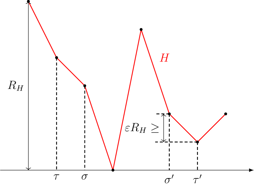
Figure 2: Explanation of (4.2) in two cases: either $\mu(\boldsymbol{\sigma})\geq\mu(\boldsymbol{\tau})$ and $H(\boldsymbol{\sigma})\leq H(\boldsymbol{\tau})$ (the left pairs), or $\mu(\boldsymbol{\sigma}^{\prime})\geq\mu(\boldsymbol{\tau}^{\prime})$ and $H(\boldsymbol{\tau}^{\prime})<H(\boldsymbol{\sigma}^{\prime})\leq H(\boldsymbol{\tau}^{\prime})+\varepsilon R_{H}$ (the right pairs).

Proposition 4.2.

Let

$$v=\sum_{\{x,y\}\in E}J_{x,y}^{2}+\sum_{x\in V}h_{x}^{2},$$ (4.4)

and recall (3.2) for the definition of $\bar{K}$. Then, $\pi^{\scriptscriptstyle\rm SCA}_{\beta,q}$ is $\varepsilon$-close to the target Gibbs $\pi^{\scriptscriptstyle\rm G}_{\beta}$ in the sense of order-preservation if

$$2q\geq\log|V|+\beta\bar{K}-\log\frac{\varepsilon\sqrt{v}}{2\bar{K}}.$$ (4.5)

Proof.

First, by (2.3), (2.5) and (2.8), we can rewrite $w^{\scriptscriptstyle\rm SCA}_{\beta,q}(\boldsymbol{\sigma})/w^{\scriptscriptstyle\rm G}_{\beta}(\boldsymbol{\sigma})$ as

$$\frac{w^{\scriptscriptstyle\rm SCA}_{\beta,q}(\boldsymbol{\sigma})}{w^{\scriptscriptstyle\rm G}_{\beta}(\boldsymbol{\sigma})} =\sum_{\boldsymbol{\tau}}\exp\bigg{(}\beta\big{(}\tilde{H}(\boldsymbol{\sigma},\boldsymbol{\sigma})-\tilde{H}(\boldsymbol{\sigma},\boldsymbol{\tau})\big{)}+q\sum_{x\in V}\sigma_{x}\tau_{x}\bigg{)}$$

$$=e^{|V|q}\sum_{I\subset V}\sum_{\boldsymbol{\tau}=\boldsymbol{\sigma}^{I}}\exp\bigg{(}\frac{\beta}{2}\sum_{x\in V}\tilde{h}_{x}(\boldsymbol{\sigma})(\tau_{x}-\sigma_{x})+q\sum_{x\in V}(\sigma_{x}\tau_{x}-1)\bigg{)}$$

$$=e^{|V|q}\sum_{I\subset V}\prod_{x\in I}e^{-\beta\tilde{h}_{x}(\boldsymbol{\sigma})\sigma_{x}-2q}=e^{|V|q}\prod_{x\in V}\big{(}1+\delta\phi_{x}(\boldsymbol{\sigma})\big{)},$$

where

$$\delta=e^{-2q}, \phi_{x}(\boldsymbol{\sigma})=e^{-\beta\tilde{h}_{x}(\boldsymbol{\sigma})\sigma_{x}}.$$ (4.6)

As a result,

$$\frac{\pi^{\scriptscriptstyle\rm SCA}_{\beta,q}(\boldsymbol{\sigma})}{\pi^{\scriptscriptstyle\rm SCA}_{\beta,q}(\boldsymbol{\tau})}=\frac{w^{\scriptscriptstyle\rm SCA}_{\beta,q}(\boldsymbol{\sigma})}{w^{\scriptscriptstyle\rm SCA}_{\beta,q}(\boldsymbol{\tau})}=\frac{w^{\scriptscriptstyle\rm G}_{\beta}(\boldsymbol{\sigma})}{w^{\scriptscriptstyle\rm G}_{\beta}(\boldsymbol{\tau})}\prod_{x\in V}\frac{1+\delta\phi_{x}(\boldsymbol{\sigma})}{1+\delta\phi_{x}(\boldsymbol{\tau})}.$$ (4.7)

Now we suppose $\pi^{\scriptscriptstyle\rm SCA}_{\beta,q}(\boldsymbol{\sigma})\geq\pi^{\scriptscriptstyle\rm SCA}_{\beta,q}(\boldsymbol{\tau})$ (cf., the former inequality in (4.2)), so that

$$\frac{w^{\scriptscriptstyle\rm G}_{\beta}(\boldsymbol{\sigma})}{w^{\scriptscriptstyle\rm G}_{\beta}(\boldsymbol{\tau})}\geq\prod_{x\in V}\frac{1+\delta\phi_{x}(\boldsymbol{\tau})}{1+\delta\phi_{x}(\boldsymbol{\sigma})}.$$ (4.8)

To prove the latter inequality in (4.2) (hence (4.3)), it suffices to show

$$\prod_{x\in V}\frac{1+\delta\phi_{x}(\boldsymbol{\tau})}{1+\delta\phi_{x}(\boldsymbol{\sigma})}\geq e^{-\beta\varepsilon R_{H}},$$ (4.9)

or equivalently

$$\beta\varepsilon R_{H}\geq\sum_{x\in V}\log\underbrace{\frac{1+\delta\phi_{x}(\boldsymbol{\sigma})}{1+\delta\phi_{x}(\boldsymbol{\tau})}}_{>0}=\sum_{x\in V}\log\bigg{(}1+\underbrace{\delta\frac{\phi_{x}(\boldsymbol{\sigma})-\phi_{x}(\boldsymbol{\tau})}{1+\delta\phi_{x}(\boldsymbol{\tau})}}_{>-1}\bigg{)}.$$ (4.10)

Next we claim that

$$R_{H}\geq\sqrt{v},$$ (4.11)

where we recall (4.4) for the definition of $v$. This is due to the fact that

$${\mathbb{E}}_{\mu}\big{[}(H-{\mathbb{E}}_{\mu}[H])^{2}\big{]}\leq R_{H}^{2}$$ (4.12)

holds for any probability measure $\mu$ on $\{\pm 1\}^{V}$, where ${\mathbb{E}}_{\mu}$ denotes the expectation against $\mu$. If $\mu$ is the uniform distribution over $\{\pm 1\}^{V}$, then

$${\mathbb{E}}_{\mu}[H] =\frac{1}{2^{|V|}}\sum_{\boldsymbol{\sigma}\in\{\pm 1\}^{V}}H(\boldsymbol{\sigma})=0,$$ (4.13)

$${\mathbb{E}}_{\mu}[H^{2}] =\frac{1}{2^{|V|}}\sum_{\boldsymbol{\sigma}\in\{\pm 1\}^{V}}H(\boldsymbol{\sigma})^{2}=v,$$ (4.14)

which yields (4.11).

Next we claim that

$$\sum_{x\in V}\log\bigg{(}1+\delta\frac{\phi_{x}(\boldsymbol{\sigma})-\phi_{x}(\boldsymbol{\tau})}{1+\delta\phi_{x}(\boldsymbol{\tau})}\bigg{)}\leq 2|V|\beta\delta\bar{K}\,e^{\beta\bar{K}},$$ (4.15)

where we recall (3.2) for the definition of $\bar{K}$. To show this, the first step is to use $\log(1+a)\leq a\leq|a|$ for all $a>-1$. Then we obtain

$$\log\bigg{(}1+\delta\frac{\phi_{x}(\boldsymbol{\sigma})-\phi_{x}(\boldsymbol{\tau})}{1+\delta\phi_{x}(\boldsymbol{\tau})}\bigg{)}\leq\bigg{|}\delta\frac{\phi_{x}(\boldsymbol{\sigma})-\phi_{x}(\boldsymbol{\tau})}{1+\delta\phi_{x}(\boldsymbol{\tau})}\bigg{|}\leq\delta|\phi_{x}(\boldsymbol{\sigma})-\phi_{x}(\boldsymbol{\tau})|.$$ (4.16)

Since $|e^{X}-e^{Y}|\leq|X-Y|(e^{X}\vee e^{Y})$ for any real $X,Y$, it is further bounded above by

$$\beta\delta\,|\tilde{h}_{x}(\boldsymbol{\sigma})\sigma_{x}-\tilde{h}_{x}(\boldsymbol{\tau})\tau_{x}|\big{(}\phi_{x}(\boldsymbol{\sigma})\vee\phi_{x}(\boldsymbol{\tau})\big{)}\leq 2\beta\delta\bar{K}\,e^{\beta\bar{K}},$$ (4.17)

which yields (4.15).

Combining the above two claims (4.11) and (4.15), we arrive at a sufficient condition for (4.10):

$$\varepsilon\sqrt{v}\geq 2|V|\delta\bar{K}\,e^{\beta\bar{K}},$$ (4.18)

which is equivalent to (4.5).  

5 Concluding remark

Propositions 3.1 and 4.2 imply the following.

Theorem 5.1.

If

$$\beta\leq\frac{1}{2\bar{K}}\log\frac{\varepsilon\sqrt{v}}{2\bar{K}},$$ (5.1)

then there is a pinning parameter $q$ for which the following both hold at the same time:

• SCA is faster than Glauber in terms of the expected number of spin-flips per update, i.e., $E^{\scriptscriptstyle\rm G}_{\beta}[|D_{\boldsymbol{\sigma},X_{\boldsymbol{\sigma}}}|]\leq E^{\scriptscriptstyle\rm SCA}_{\beta,q}[|D_{\boldsymbol{\sigma},X_{\boldsymbol{\sigma}}}|]$ for any $\boldsymbol{\sigma}\in\{\pm 1\}^{V}$.

• The SCA equilibrium $\pi^{\scriptscriptstyle\rm SCA}_{\beta,q}$ is $\varepsilon$-close to the target Gibbs $\pi^{\scriptscriptstyle\rm G}_{\beta}$ in the sense of order-preservation. In particular, if $\pi^{\scriptscriptstyle\rm SCA}_{\beta,q}$ takes on its highest point at $\boldsymbol{\sigma}$, then $H(\boldsymbol{\sigma})\leq H(\boldsymbol{\tau})+\varepsilon R_{H}$ holds for all $\boldsymbol{\tau}\in\{\pm 1\}^{V}$.

The main message of the above theorem is that, to ensure the above two properties simultaneously, we have to keep the temperature sufficiently high. However, if the temperature is too high (e.g., $\beta=0$), then the equilibrium distributions are almost identical to the uniform distribution over $\{\pm 1\}^{V}$, which is not at all efficient to search for the ground states. In this respect, we want to take the largest possible value of $\beta$.

The upper bound in (5.1) depends on the coupling coefficients $\{J_{x,y}\}_{\{x,y\}\in E}$ and $\{h_{x}\}_{x\in V}$ as well as the graph structure $G=(V,E)$. Suppose that the coupling coefficients are uniformly bounded (e.g., $J_{x,y},h_{x}\in\{\pm 1\}$). If $G$ is a regular graph with bounded degree (e.g., a subset of the square lattice), then the bound in (5.1) is of order $\log|V|$, which is better than the bound obtained by Dobrushin’s condition (e.g., [2]) in a large volume, and we may find a good candidate for the ground states of a large system via a sufficiently slow cooling method $\beta\to\infty$, such as simulated annealing [1, 6]. On the other hand, if $G$ is a complete graph, then the bound in (5.1) is finite (or, even worse, may be negative) and therefore the two properties in Theorem 5.1 may not hold at the same time under any cooling methods (see [11] for application of SCA to the SK spin glass).

Instead of taking $\beta$ to infinity, we should keep $\beta$ bounded as in (5.1). Since $\pi^{\scriptscriptstyle\rm SCA}_{\beta,q}$ (supposed to be close to $\pi^{\scriptscriptstyle\rm G}_{\beta}$) is not concentrated on the ground states, the chance of a single MCMC experiment hitting a ground states is slim. Instead, we may have to run $N$ independent MCMCs $\{X_{j}\}_{j=1}^{N}$ whose common law is $U*(P^{\scriptscriptstyle\rm SCA}_{\beta,q})^{*n}$, where $U$ is the uniform distribution over $\{\pm 1\}^{V}$, and construct a profile $\frac{1}{N}\sum_{j=1}^{N}\delta_{X_{j}}$ that is supposed to be close to $\pi^{\scriptscriptstyle\rm SCA}_{\beta,q}$ (hence to $\pi^{\scriptscriptstyle\rm G}_{\beta}$) if $n$ and $N$ are sufficiently large. Then, a ground state may be captured as $\arg\max\frac{1}{N}\sum_{j=1}^{N}\delta_{X_{j}}$. How large $n$ has to be depends on the mixing time, which is under investigation with Bruno Kimura. On the other hand, how large $N$ has to be depends on the convergence rate in the law of large numbers (LLN). Sanov’s theorem [10] gives the exact exponential rate of convergence, but the multiplicative term could be huge (in powers of $N$) depending on the degree of degeneracy. This is partly due to the fact that the number $2^{|V|}$ of spin configurations is way larger than the number $N$ of experiments, which is not in the regime of LLN. We are currently seeking to apply a theory of big data: high-dimensional statistics [4].

References

- [1] V. Černý. Thermodynamical approach to the traveling salesman problem: an efficient simulation algorithm. J. Optimiz. Theory App., 45 (1985): 41–51.
- [2] P. Dai Pra, B. Scoppola and E. Scoppola. Sampling from a Gibbs measure with pair interaction by means of PCA. J. Stat. Phys., 149 (2012): 722–737.
- [3] M.R. Garey and D.S. Johnson. Computers and Intractability: A Guide to the Theory of NP-Completeness. W.H. Freeman and Company, San Francisco (1979).
- [4] C. Giraud. Introduction to High-Dimensional Statistics. Chapman & Hall/CRC, Boca Raton (2015).
- [5] R.J. Glauber. Time-dependent statistics of the Ising Model. J. Math. Phys., 4 (1963): 294–307.
- [6] S. Kirkpatrick, C.D. Gelatt Jr., M.P. Vecchi. Optimization by simulated annealing. Science, New Series, 220 (1983): 671–680.
- [7] D.A. Levin, Y. Peres and E.L. Wilmer. Markov Chains and Mixing Times. AMS, Providence, Rhode Island (2009).
- [8] A. Lucas. Ising formulations of many NP problems. Front. Phys., 12 (2014): https://doi.org/10.3389/fphy.2014.00005.
- [9] M. Normann, A. Sakai, H. Toyokawa and Y. Ueda. Stability of energy landscape. In preparation.
- [10] I.N. Sanov. On the probability of large deviations of random variables. Mat. Sbornik, 42 (1957): 11–44. English translation in Sel. Transl. Math. Stat. Prob., 1 (1961): 213–244.
- [11] B. Scoppola and A. Troiani. Gaussian mean field lattice gas. J. Stat. Phys., 170 (2018): 1161–1176.