Second-order multi-object filtering with target interaction using determinantal point processes

Abstract

The Probability Hypothesis Density (PHD) filter, which is used for multi-target tracking based on sensor measurements, relies on the propagation of the first-order moment, or intensity function, of a point process. This algorithm assumes that targets behave independently, an hypothesis which may not hold in practice due to potential target interactions. In this paper, we construct a second-order PHD filter based on Determinantal Point Processes (DPPs) which are able to model repulsion between targets. Such processes are characterized by their first and second-order moments, which allows the algorithm to propagate variance and covariance information in addition to first-order target count estimates. Our approach relies on posterior moment formulas for the estimation of a general hidden point process after a thinning operation and a superposition with a Poisson Point Process (PPP), and on suitable approximation formulas in the determinantal point process setting. The repulsive properties of determinantal point processes apply to the modeling of negative correlation between distinct measurement domains. Monte Carlo simulations with correlation estimates are provided.

Keywords: Probability hypothesis density (PHD) filter; higher-order statistics; correlation; second-order moment; determinantal point processes; multi-object filtering; multi-target tracking.

Mathematics Subject Classification (2010): 60G35; 60G55; 62M30; 62L12.

1 Introduction

Probability Hypothesis Density (PHD) filters have been introduced in Mahler (2003) for multi-target tracking in cluttered environments. The construction of the prediction point process $\Phi$ therein uses multiplicative point processes, see e.g. Moyal (1962), Moyal (1964), by thinning and shifting a prior point process $\Psi$, and superposition with a birth point process. The posterior point process $\Phi|\Xi$ is obtained by conditioning $\Phi$ given a measurement point process of targets $\Xi$, also constructed by thinning, shifting and superposition. This step relies on Bayesian estimation with a Poisson point process prior, see e.g. van Lieshout (1995), Mori (1997), Portenko et al. (1997). PHD filters have low complexity, and they allow for explicit update formulas see e.g. Clark et al. (2016) for a review.

While the PHD filter of Mahler (2003) is based on Poisson point processes, several extensions of the PHD filter to non-Poisson prior distributions have been proposed. Cardinalized Probability Hypothesis Density (CPHD) filters have been introduced in Mahler (2007) as a generalization in which the target count is allowed to have an arbitrary distribution. In de Melo and Maskell (2019), discretized Gamma distributions are used to design an efficient approximation of the CPHD filter cardinality distribution. Other generalizations include the Gauss-Poisson point processes that generalize the Poisson point process by allowing for two-point clusters, and have been used in Singh et al. (2009). The PHD filter has been implemented using the Sequential Monte Carlo (SMC) method in Vo et al. (2005), and using Gaussian mixtures in Vo and Ma (2006).

PHD filters approximate the distribution of the number of targets by a Poisson distribution estimated by a single mean (or variance) parameter, which can result into high variance estimates when the estimated mean is high. Second-order PHD filters that can propagate distinct information on mean and variance parameters have been recently proposed in Schlangen et al. (2018), based on the Panjer point process defined therein, where the Panjer cardinality distribution encompasses the binomial, Poisson and negative binomial distributions. Other multi-target filters propagating second-order moment information have also been recently proposed, see e.g. Clark and de Melo (2018) for a filter that propagates second-order point process factorial cumulants.

A common feature of cardinalized filters is to assume that target locations are distributed as $n$ independent random samples according to a reference intensity measure, given that the observation window contains $n$ points. While this hypothesis is natural and facilitates an explicit derivation of prediction formulas, it does not reflect potential interaction between targets. In addition, as observed in the simulations of Section 6, the presence of repulsion between targets can degrade the performance of the Poisson PHD filter.

As a response, we propose to construct a PHD filter based on determinantal point processes introduced in Macchi (1975), which are able to model repulsion among configuration points on a target domain $\Lambda\subset{\mathord{\mathbb{R}}}^{d}$, see also Soshnikov (2000) and Shirai and Takahashi (2003). Taking into account correlation via more general point process-based PHD filters poses several challenges linked to the derivation of closed form filtering formulas. In addition, the distribution of general point processes relies on Janossy densities which may not be characterized by the knowledge of a finite number of moments. Determinantal point processes, on the other hand, are characterized by their kernel functions $(K(x,y))_{(x,y)\in\Lambda^{2}}$, and their Janossy densities can be recovered from their first and second-order moments. In this setting, the knowledge of first and second-order moments can be used to update the Janossy densities that characterize the underlying determinantal point process.

Discrete determinantal point processes have also been recently used for the pruning of Gaussian components in the Gaussian Mixture (GM) PHD filter in Jorquera et al. (2019), see also Jorquera et al. (2018) for other applications to multi-target tracking. Permanental processes have been used in Mahler (2015) to propagate a joint Poisson distribution, however this approach is distinct from the determinantal setting. See Koch (2018) for the use the exclusion principle in multi-target tracking by a fermionic filtering update of anti-symmetric components in the joint probability density functions of states. Note also that determinantal point processes have been originally introduced in Macchi (1975) to represent configurations of fermions.

After recalling general facts and notation on point processes in Section 2, we derive general formulas for the distribution, and for the first and second-order moments, of a posterior point process $\Phi|\Xi$ in Section 3, see also Lund and Rudemo (2000). In Section 4 we review the construction of determinantal point processes, and in Section 5 we present a second-order PHD filtering algorithm based on determinantal point processes, with the computation of the prediction kernel $K_{\Phi}(x,y)$ and of the updated kernel $K_{\Phi\mid\Xi}(x,y)$. An implementation of the Poisson PHD filter that allows for performance evaluation using measurement-estimate associations is presented in Section 6 with numerical illustrations. This simulation is based on the sequential Monte Carlo (or particle filtering) method with a nearly constant turn-rate motion dynamics, see Vo et al. (2009), Li et al. (2017), to which we add a repulsion term. In Section 7 we implement the determinantal PHD filter using the sequential Monte Carlo method. The implementation of the algorithm relies on closed-form filter update expressions obtained from approximation formulas for corrector terms and Janossy densities presented in appendix.

2 Preliminaries on point processes

In this section we review the properties of point processes; see, e.g. Daley and Vere-Jones (2003), Decreusefond et al. (2016), and references therein. For any subset $A\subseteq{\mathord{\mathbb{R}}}^{d}$, let $|A|$ denote the cardinality of $A$, setting $|A|=\infty$ if $A$ is not finite, and let

$$\mathbf{N}_{\sigma}:=\{\xi\subseteq{\mathord{\mathbb{R}}}^{d}\ :\ |\xi\cap A|<\infty\quad\text{ for all relatively compact sets }A\subset{\mathord{\mathbb{R}}}^{d}\}$$

denote the set of locally finite point configurations on ${\mathord{\mathbb{R}}}^{d}$, which is identified with the set of all nonnegative integer-valued Radon measures $\xi$ on ${\mathord{\mathbb{R}}}^{d}$ such that $\xi(\{x\})\in\{0,1\}$ for all $x\in{\mathord{\mathbb{R}}}^{d}$. We denote by ${\mathscr{N}_{\sigma}}$ the Borel $\sigma$-field generated by the weakest topology that makes the mappings

$$\xi\mapsto\langle f,\xi\rangle:=\sum_{y\in\xi}f(y)$$

continuous for all continuous and compactly supported functions $f$ on ${\mathord{\mathbb{R}}}^{d}$. Given $\Lambda$ a relatively compact subset of ${\mathord{\mathbb{R}}}^{d}$, we let $\mathbf{N}_{\sigma}(\Lambda)$ be the space of finite configurations on $\Lambda$.

We consider a simple and locally finite point process $\Phi$ on $\Lambda$, defined as a random element on a probability space $(\Omega,{\mathscr{N}_{\sigma}})$ with values in $\mathbf{N}_{\sigma}(\Lambda)$, and denote its distribution by ${\mathbb{P}}$. The point process $\Phi$ is characterized by its Laplace transform $\mathcal{L}_{\Phi}$ which is defined, for any measurable nonnegative function $f$ on ${\Lambda}$, by

$$\mathcal{L}_{\Phi}(f)=\int_{\mathbf{N}_{\sigma}}e^{-\langle f,\xi\rangle}\,{\mathbb{P}}(d\xi).$$ (2.1)

We denote the expectation of an integrable random variable $F$ defined on $(\mathbf{N}_{\sigma},{\mathscr{N}_{\sigma}},{\mathbb{P}})$ by

$$\mathop{\hbox{\rm I\kern-1.99997ptE}}\nolimits[F(\Phi)]:=\int_{{\mathbf{N}_{\sigma}}}F(\xi)\,{\mathbb{P}}(d\xi).$$

Janossy densities

For any relatively compact subset $A\subseteq{\Lambda}$, the Janossy densities of $\Phi$ w.r.t. a reference Radon measure ${\nu}$ on ${\Lambda}$ are symmetric measurable functions $j^{(n)}_{\Lambda}:\Lambda^{n}\rightarrow[0,\infty)$ satisfying

$$\mathop{\hbox{\rm I\kern-1.99997ptE}}\nolimits\left[F(\mathbb{\Phi})\right]=F(\emptyset)\,j_{\Lambda}^{(0)}+\sum_{n\geq 1}\frac{1}{n!}\int_{\Lambda^{n}}F(\{x_{1},\ldots,x_{n}\})\,j_{\Lambda}^{n}\left(x_{1},\ldots,x_{n}\right)\,{\nu}(dx_{1})\cdots{\nu}(dx_{n}),$$

for all measurable functions $F:\mathbf{N}_{\sigma}(\Lambda)\rightarrow[0,\infty)$; see, e.g., Georgii and Yoo (2005).

For $n\geq 1$, the Janossy density $j^{(n)}_{\Lambda}(x_{1},\ldots,x_{n})$ is proportional, up to a multiplicative constant, to the joint density of the $n$ points of the point process, given that it has exactly $n$ points. For $n=0$, $j^{(0)}_{\Lambda}(\emptyset)$ is the probability that there are no points in $\Lambda$.

Correlation functions

The correlation functions of $\Phi$ w.r.t. the reference measure ${\nu}$ on ${\Lambda}$ are measurable symmetric functions $\rho^{(k)}_{\Phi}:{\Lambda}^{k}\longrightarrow[0,\infty)$ such that

$$\mathop{\hbox{\rm I\kern-1.99997ptE}}\nolimits\left[\prod_{i=1}^{k}\mathbb{\Phi}(B_{i})\right]=\int_{B_{1}\times\cdots\times B_{k}}\rho^{(k)}_{\Phi}(x_{1},\ldots,x_{k})\,{\nu}(dx_{1})\cdots{\nu}(dx_{k}),$$ (2.2)

for any family of mutually disjoint bounded subsets $B_{1},\ldots,B_{k}$ of ${\Lambda}$, $k\geq 1$. More generally, if $B_{1},\ldots,B_{n}$ are disjoint bounded Borel subsets of ${\Lambda}$ and $k_{1},\ldots,k_{n}$ are integers such that $\sum_{i=1}^{n}k_{i}=N$, we have

$$\mathop{\hbox{\rm I\kern-1.99997ptE}}\nolimits\left[\prod_{i=1}^{n}\frac{\Phi(B_{i})!}{(\Phi(B_{i})-k_{i})!}\right]=\int_{B_{1}^{k_{1}}\times\cdots\times B_{n}^{k_{n}}}\rho^{(N)}_{\Phi}(x_{1},\ldots,x_{N})\,{\nu}(dx_{1})\cdots{\nu}(dx_{N}).$$

In addition, we let $\rho^{(n)}_{\Phi}(x_{1},\ldots,x_{n})=0$ whenever $x_{i}=x_{j}$ for some $1\leq i\neq j\leq n$. In other words, the factorial moment density $\rho^{(n)}_{\Phi}(x_{1},\ldots,x_{n})$ of $\Phi$, $x_{1},\ldots,x_{n}\in\Lambda$, $x_{i}\not=x_{j}$, $1\leq i<j\leq n$, is defined from the relation

$$\int_{B_{1}\times\cdots\times B_{n}}\rho^{(n)}_{\Phi}(x_{1},\ldots,x_{n})\nu(dx_{1})\cdots\nu(dx_{n})=\mathop{\hbox{\rm I\kern-1.99997ptE}}\nolimits\left[\sum_{x_{1},\ldots,x_{n}\in\Phi}{\bf 1}_{B_{1}}(x_{1})\cdots{\bf 1}_{B_{n}}(x_{n})\right],$$

for mutually disjoint measurable subsets $B_{1},\ldots,B_{n}\subset\Lambda$, where ${\bf 1}_{B_{i}}$ denotes the indicator function over $B_{i}$, $i=1,\ldots,n$. Heuristically, $\rho^{(n)}_{\Phi}(x_{1},\ldots,x_{n})\,{\nu}(dx_{1})\cdots{\nu}(dx_{n})$ represents the probability of finding a particle in the vicinity of each $x_{i}$, $i=1,\ldots,n$.

We also recall that the Janossy densities $j^{(n)}_{\Lambda}$ can be recovered from the correlation functions $\rho^{(m)}_{\Phi}$ via the relation

$$j^{(n)}_{\Lambda}(x_{1},\ldots,x_{n})=\sum_{m\geq 0}\frac{(-1)^{m}}{m!}\int_{\Lambda^{m}}\rho^{(n+m)}_{\Phi}(x_{1},\ldots,x_{n},y_{1},\ldots,y_{m})\,{\nu}(dy_{1})\cdots{\nu}(dy_{m}),$$

and vice versa using the equality

$$\rho^{(n)}_{\Phi}(x_{1},\ldots,x_{n})=\sum_{m\geq 0}\frac{1}{m!}\int_{\Lambda^{m}}j^{(m+n)}_{\Lambda}(x_{1},\ldots,x_{n},y_{1},\ldots,y_{m})\,{\nu}(dy_{1})\cdots{\nu}(dy_{m}),$$

see Theorem 5.4.II of Daley and Vere-Jones (2003).

Probability generating functionals

The Probability Generating Functional (PGFl) of the point process $\Phi$, see Moyal (1962), is defined by

$${h\mapsto{\cal G}_{\Phi}(h)} := {\mathop{\hbox{\rm I\kern-1.99997ptE}}\nolimits\left[\prod_{i=1}^{\Phi(\Lambda)}h(X_{i})\right]}$$

$$= {j^{(0)}_{\Phi}+\sum_{n\geq 1}\frac{1}{n!}\int_{\Lambda^{n}}j^{(n)}_{\Phi}(x_{1},\ldots,x_{n})\prod_{i=1}^{n}h(x_{i})\ \!\nu(dx_{1})\cdots\nu(dx_{n}),}$$

for $h\in L^{\infty}(\Lambda)$ a bounded measurable function on $\Lambda$. Given ${\cal F}$ a functional on $L^{\infty}(\Lambda)$, we will use the functional derivative $\partial_{g}/\partial h$ of ${\cal F}(h)$ in the direction of $g\in L^{\infty}(\Lambda)$, defined as

$$\frac{\partial_{g}}{\partial h}{\cal F}(h):=\lim_{\varepsilon\to 0}\frac{{\cal F}(h+\varepsilon g)-{\cal F}(h)}{\varepsilon}.$$

Given $x\in\Lambda$, we also let

$$\frac{\partial_{\delta_{x}}}{\partial h}{\cal F}(h):=\lim_{n\to\infty}\frac{\partial_{g_{n}}}{\partial h}{\cal F}(h),$$ (2.3)

where $(g_{n})_{n\geq 1}$ is a sequence of bounded functions converging weakly to the Dirac distribution $\delta_{x}$ at $x\in\Lambda$.

This construction allows one to recover the Janossy densities $j^{(n)}_{\Phi}(x_{1},\ldots,x_{n})$ and factorial moment densities $\rho^{(n)}_{\Phi}(x_{1},\ldots,x_{n})$ of $\Phi$ from the PGFl ${\cal G}_{\Phi}(h)$ as

$${j^{(n)}_{\Phi}(x_{1},\ldots,x_{n})=\frac{\partial_{\delta_{x_{1}}}}{\partial h}\cdots\frac{\partial_{\delta_{x_{n}}}}{\partial h}{\cal G}_{\Phi}(h)_{\mid h=0},\quad x_{1},\ldots,x_{n}\in\Lambda,}$$ (2.4)

see e.g. § 2.4 of Clark et al. (2016), and as

$${\rho^{(n)}_{\Phi}(x_{1},\ldots,x_{n})=\frac{\partial_{\delta_{x_{1}}}}{\partial h}\cdots\frac{\partial_{\delta_{x_{n}}}}{\partial h}{\cal G}_{\Phi}(h)_{\mid h=1},\quad x_{1},\ldots,x_{n}\in\Lambda,}$$ (2.5)

with $x_{i}\not=x_{j}$, $1\leq i<j\leq n$; see, e.g., § 3.4 of Clark et al. (2016).

3 Posterior point process distribution

In this section we compute the Janossy densities, and the first and second-order moments, of a posterior point process of targets $\Phi$ given the point process $\Xi$ of sensor measurements. The case of a Poisson prior was treated in Chapter 5 of van Lieshout (1995), see Theorem 29 therein and also Mori (1997) for early sensor fusion applications, or Theorems 6.1-6.2 Portenko et al. (1997) for related derivations based on Laplace transforms.

In Propositions 3.2 and 3.3 below we will use extensions of the corrector terms $l^{(1)}_{z_{1:m}}$, $l^{(2)}_{z_{1:m}}$ introduced in Delande et al. (2014) for the cardinalized PHD filter, see Vo et al. (2007). We start with a review of the thinning and shifting of point processes; see, e.g., Clark et al. (2016) and references therein for details.

Thinning and shifting of point processes

The point process $\Xi$ of sensor measurements is constructed via the following steps.

1. Thinning and shifting. Every target point $x\in\Phi$ is kept with probability $p_{d}(x)\in(0,1]$ and shifted according to the probability density function $l_{d}(\cdot|x)$, by branching the hidden point process $\Phi$ with a Bernoulli point process $\Xi_{s}$ with PGFl

   $$g\mapsto{\cal G}_{\Xi_{s}}(g\mid x) := q_{d}(x)+p_{d}(x)\int_{\Lambda}g(z)l_{d}(z|x)\nu(dz)$$ (3.1)

   $$= q_{d}(x)+\int_{\Lambda}g(z)\tilde{l}_{d}(z|x)\nu(dz),$$

   where for compactness of notation we take

   $$q_{d}(x):=1-p_{d}(x)\quad\mbox{and}\quad\tilde{l}_{d}(z|x):=p_{d}(x)l_{d}(z|x),\quad x\in\Lambda.$$ (3.2)

2. The point process $\Xi$ is obtained by superposing a Poisson point process $\Xi_{c}$ with intensity function $l_{c}(\cdot)$, representing clutter, to the above thinning and shifting of $\Phi$.

In the sequel we use the shorthand notation

$$x_{1:n}=(x_{1},\ldots,x_{n})\in\Lambda^{n},\quad\mbox{and}\quad\nu(dx_{1:n}):=\nu(dx_{1})\cdots\nu(dx_{n}),$$

with $x_{1:0}=\emptyset$; see Delande et al. (2014), Schlangen et al. (2018). The joint PGFl of the point process $(\Phi,\Xi)$ is given by

$$(h,g)\mapsto{\cal G}_{\Phi,\Xi}(h,g):={\cal G}_{\Xi_{c}}(g){\cal G}_{\Phi}\big{(}h(\cdot){\cal G}_{\Xi_{s}}(g\mid\cdot\ \!)\big{)},$$ (3.3)

see, e.g., Theorem 1.1 of Moyal (1964) where, taking $p_{d}(x):=p_{d}$ for simplicity, $x\in\Lambda$, we have

$${\cal G}_{\Phi}\big{(}h(\cdot){\cal G}_{\Xi_{s}}(g\mid\cdot\ \!)\big{)} =\sum_{n\geq 0}\frac{1}{n!}\int_{\Lambda^{n}}j^{(n)}_{\Phi}(x_{1:n}){\prod_{i=1}^{n}\left(h(x_{i})\left(q_{d}+\int_{\Lambda}g(z)\tilde{l}_{d}(z|x_{i})\nu(dz)\right)\right)\nu(dx_{1:n})}$$

$$={\sum_{n\geq 0}\frac{1}{n!}\int_{\Lambda^{n}}j^{(n)}_{\Phi}(x_{1:n})\prod_{j=1}^{n}h(x_{j})}{\sum_{k=0}^{n}{n\choose k}q_{d}^{n-k}\prod_{i=1}^{k}\int_{\Lambda}g(z)\tilde{l}_{d}(z|x_{i})\nu(dz)\nu(dx_{1:n})}$$

$$={\sum_{k\geq 0}\int_{\Lambda^{k}}\prod_{i=1}^{k}\int_{\Lambda}g(z)\tilde{l}_{d}(z|x_{i})\nu(dz)}{\sum_{n\geq 0}\frac{q_{d}^{n}}{n!k!}\int_{\Lambda^{n}}j^{(k+n)}_{\Phi}(x_{1:k+n})\prod_{j=1}^{k+n}h(x_{j})\nu(dx_{1:k+n}).}$$

The marginal PGFl of the point process $\Xi$ is given by

$$g\mapsto{\cal G}_{\Xi}(g) = {\cal G}_{\Phi,\Xi}({\bf 1},g)$$ (3.4)

$$= {\cal G}_{\Xi_{c}}(g){\cal G}_{\Phi}\big{(}{\cal G}_{\Xi_{s}}(g\mid\cdot\ \!)\big{)}$$

$$= \mathcal{G}_{\Xi_{c}}(g)\mathcal{G}_{\Phi}\left(q_{d}(\cdot)+\int_{\Lambda}g(y)\tilde{l}_{d}(y\ \!|\ \!\cdot)\nu(dy)\right).$$

Marginal moments of $\Xi$

The first derivative of $\mathcal{G}_{\Xi}(g)$ is given by

$$\frac{\partial_{\delta_{x}}}{\partial g}\mathcal{G}_{\Xi}(g) = \frac{\partial_{\delta_{x}}}{\partial g}\big{(}\mathcal{G}_{\Phi}(\mathcal{G}_{\Xi_{s}}(g\mid\cdot))\mathcal{G}_{\Xi_{c}}(g)\big{)}$$

$$= \mathcal{G}_{\Xi_{c}}(g)\frac{\partial_{\delta_{x}}}{\partial g}\mathcal{G}_{\Phi}(\mathcal{G}_{\Xi_{s}}(g\mid\cdot)+\mathcal{G}_{\Phi}(\mathcal{G}_{\Xi_{s}}(g\mid\cdot))\frac{\partial_{\delta_{x}}}{\partial g}\mathcal{G}_{\Xi_{c}}(g)$$

$$= \mathcal{G}_{\Xi_{c}}(g)\frac{\partial_{\delta_{x}}}{\partial g}\mathcal{G}_{\Phi}\left(q_{d}(\cdot)+\int_{\Lambda}g(y)\tilde{l}_{d}(y\ \!|\ \!\cdot)\nu(dy))\right)$$

$$+\mathcal{G}_{\Phi}\left(q_{d}(\cdot)+\int_{\Lambda}g(y)\tilde{l}_{d}(y\ \!|\ \!\cdot)\nu(dy)\right)\frac{\partial_{\delta_{x}}}{\partial g}\mathcal{G}_{\Xi_{c}}(g),$$

from which the first-order moment density of $\Xi$ can be computed after setting $g=1$ as

$${\mu^{(1)}_{\Xi}(x)=\frac{\partial_{\delta_{x}}}{\partial g}\mathcal{G}_{\Xi}(g)_{\mid g=1}=\mu^{(1)}_{\Xi_{c}}(x)+\int_{\Lambda}\tilde{l}_{d}(x|y)\mu^{(1)}_{\Phi}(y)\nu(dy).}$$ (3.5)

Similarly, the second derivative of $\mathcal{G}_{\Xi}(g)$ is given by

$${\frac{\partial_{\delta_{x}}}{\partial g}\frac{\partial_{\delta_{y}}}{\partial g}\bigg{(}\mathcal{G}_{\Phi}(\mathcal{G}_{\Xi_{s}}(g\mid\cdot))\mathcal{G}_{\Xi_{c}}(g)\bigg{)}} ={\mathcal{G}_{\Xi_{c}}(g)\frac{\partial_{\delta_{x}}}{\partial g}\frac{\partial_{\delta_{y}}}{\partial g}\mathcal{G}_{\Phi}(\mathcal{G}_{\Xi_{s}}(g\mid\cdot))+\frac{\partial_{\delta_{x}}}{\partial g}\mathcal{G}_{\Phi}(\mathcal{G}_{\Xi_{s}}(g\mid\cdot))\frac{\partial_{\delta_{y}}}{\partial g}\mathcal{G}_{\Xi_{c}}(g)}$$

$${\quad+\frac{\partial_{\delta_{y}}}{\partial g}\mathcal{G}_{\Phi}(\mathcal{G}_{\Xi_{s}}(g\mid\cdot))\frac{\partial_{\delta_{x}}}{\partial g}\mathcal{G}_{\Xi_{c}}(g)+\mathcal{G}_{\Phi}(\mathcal{G}_{\Xi_{s}}(g\mid\cdot))\frac{\partial_{\delta_{x}}}{\partial g}\frac{\partial_{\delta_{y}}}{\partial g}(\mathcal{G}_{\Xi_{c}}(g)),}$$

from which the second-order factorial moment density of $\Xi$ can be computed after setting $g=1$ as

$$\rho^{(2)}_{\Xi}(x,y) = \int_{\Lambda^{2}}\tilde{l}_{d}(x|u)\tilde{l}_{d}(y|v)\rho^{(2)}_{\Phi}(u,v)\nu(du)\nu(dv)+\rho^{(2)}_{\Xi_{c}}(x,y)$$

$${+\mu^{(1)}_{\Xi_{c}}(y)\int_{\Lambda}\tilde{l}_{d}(x|u)\mu^{(1)}_{\Phi}(u)\nu(du)}{+\mu^{(1)}_{\Xi_{c}}(x)\int_{\Lambda}\tilde{l}_{d}(y|v)\mu^{(1)}_{\Phi}(v)\nu(dv),}$$

$x,y\in\Lambda$, $x\not=y$.

Posterior distribution

In Lemma 3.1 below, we derive the general expression of the Janossy densities of the posterior point process $\Phi|\Xi$ given the sensor measurements $\Xi$. In the sequel, we let $|S|$ denote the cardinality of subsets $S\subset\{1,\ldots,m\}$, and we use the notation $z_{1:m}=(z_{1},\ldots,z_{n})$, while $z_{1:m}\setminus z$ denotes the sequence $(z_{1},\ldots,z_{n})$ with the omission of $z$ if $z\in\{z_{1},\ldots,z_{n}\}$.

Lemma 3.1

The $n$-th conditional Janossy density of $\Phi$ given that $\Xi=z_{1:m}=(z_{1},\ldots,z_{m})$ satisfies

$$j^{(n)}_{\Phi\mid\Xi=z_{1:m}}(x_{1},\ldots,x_{n})=\frac{j^{(n,m)}_{\Phi,\Xi=z_{1:m}}(x_{1},\ldots,x_{n})}{j^{(m)}_{\Xi}(z_{1:m})},\qquad x_{1},\ldots,x_{n}\in\Lambda,$$ (3.7)

$m,n\geq 0$, where
$(i)$ the $(n,m)$-th joint Janossy density of $(\Phi,\Xi)$ is given by

$$j^{(n,m)}_{\Phi,\Xi=z_{1:m}}(x_{1},\ldots,x_{n})={j^{(n)}_{\Phi}(x_{1},\ldots,x_{n})}{\sum_{S\subset\{1,\ldots,m\}\atop|S|\leq n}\frac{n!q_{d}^{n-|S|}}{(n-|S|)!}\prod_{j\notin S}l_{c}(z_{j})\sum_{\pi:S\rightarrow\{1,\ldots,n\}}\prod_{i\in S}\tilde{l}_{d}(z_{i}|x_{\pi(i)}),}$$ (3.8)

the above sum being over injective mappings $\pi:S\rightarrow\{1,\ldots,n\}$, and
$(ii)$ the Janossy densities of the measurement point process $\Xi$ are given by

$${j^{(m)}_{\Xi}(z_{1},\ldots,z_{m})=\sum_{n\geq 0}\sum_{S\subset\{1,\ldots,m\}\atop|S|\leq n}}{\prod_{j\notin S}l_{c}(z_{j})\frac{q_{d}^{n-|S|}}{(n-|S|)!}\int_{\Lambda^{n}}j^{(n)}_{\Phi}(x_{1:n})\prod_{i\in S}\tilde{l}_{d}(z_{i}|x_{i})\nu(dx_{1:n}),}$$ (3.9)

$m\geq 0$.

Proof. In order to derive the $(n,m)$-th joint Janossy density of $(\Phi,\Xi)$ as in (2.4), we need to compute

$$\frac{\partial_{\eta_{1}}}{\partial h}\cdots\frac{\partial_{\eta_{n}}}{\partial h}\frac{\partial_{f_{1}}}{\partial g}\cdots\frac{\partial_{f_{m}}}{\partial g}\mathcal{G}_{\Phi,\Xi}(h,g)$$

in the directions of the functions $\eta_{1},\ldots,\eta_{n}$, $f_{1},\ldots,f_{m}\in L^{\infty}(\Lambda)$. For a given set $S\subseteq\{1,\ldots,m\}$ we let $\pi:=\left|S\right|$ and denote the elements of $S$ as $S(1),\ldots,S(\pi)$ in increasing order, where $S$ is identified to the mapping $S:\{1,\ldots,\pi\}\rightarrow\{1,\ldots,m\}$. By the Faà di Bruno’s formula, see, e.g., Clark and Houssineau (2012), and (3.3), we have

$$\frac{\partial_{f_{1}}}{\partial g}\cdots\frac{\partial_{f_{m}}}{\partial g}\mathcal{G}_{\Phi,\Xi}(h,g)=\frac{\partial_{f_{1}}}{\partial g}\cdots\frac{\partial_{f_{m}}}{\partial g}\big{(}\mathcal{G}_{\Xi_{c}}(g)\mathcal{G}_{\Phi}(h(\cdot)\mathcal{G}_{\Xi_{s}}(g\ \!|\ \!\cdot))\big{)}$$

$$=\sum_{\begin{subarray}{c}S\subseteq\{1,\ldots,m\}\\ \pi=\left|S\right|\\ Q\subset\{1,\ldots,m\}\backslash S\end{subarray}}\left(\frac{\partial_{f_{S(1)}}}{\partial g}\cdots\frac{\partial_{f_{S(\pi)}}}{\partial g}\mathcal{G}_{\Phi}(h(\cdot)\mathcal{G}_{\Xi_{s}}(g\ \!|\ \!\cdot))\right)\left(\frac{\partial_{f_{Q(1)}}}{\partial g}\cdots\frac{\partial_{f_{Q(m-\pi)}}}{\partial g}\mathcal{G}_{\Xi_{c}}(g)\right),$$ (3.10)

where the index set $S\subseteq\{1,\ldots,m\}$ runs through the collection of $2^{m}$ subsets of $\{1,\ldots,m\}$. Next, the $m^{\text{th}}$ derivative of $\mathcal{G}_{\Phi}(h(\cdot)\mathcal{G}_{\Xi_{s}}(g\ \!|\ \!\cdot))$ can be computed by a standard induction argument as

$$\frac{\partial_{f_{1}}}{\partial g}\cdots\frac{\partial_{f_{m}}}{\partial g}\mathcal{G}_{\Phi}(h(\cdot)\mathcal{G}_{\Xi_{s}}(g\ \!|\ \!\cdot))$$ (3.11)

$$=\sum_{a=m}^{\infty}\frac{1}{a!}\int_{\Lambda^{a}}j_{\Phi}^{(a)}(u_{1:a})\hskip-5.69046pt\sum_{\begin{subarray}{c}s_{1},\ldots,s_{m}=1\\ s_{1}\neq\cdots\neq s_{m}\end{subarray}}^{a}\prod_{l=1}^{m}\Big{(}h(u_{s_{l}})\int_{\Lambda}f_{l}(z)\tilde{l}_{d}(z|u_{s_{l}})\nu(dz)\Big{)}\hskip-14.22636pt\prod_{s\in\{1,\ldots,a\}\backslash\{s_{1},\ldots,s_{m}\}}^{a}\hskip-28.45274pt\big{(}h(u_{s})\mathcal{G}_{\Xi_{s}}(g|u_{s})\big{)}\nu(du_{1:a}).$$

Substituting $f_{1},\ldots,f_{m}$ with Dirac delta functions $\delta_{z_{1}},\ldots,\delta_{z_{m}}$ at the distinct configuration points $z_{1:m}\in\Lambda$ as in (2.3) and setting $g=0$ in (3.11), we find

$$\frac{\partial_{\delta_{z_{1}}}}{\partial g}\cdots\frac{\partial_{\delta_{z_{m}}}}{\partial g}\mathcal{G}_{\Phi}(h(\cdot)\mathcal{G}_{\Xi_{s}}(g\ \!|\ \!\cdot))_{|g=0} =\sum_{a=m}^{\infty}\frac{q_{d}^{a-m}}{a!}\int_{\Lambda^{a}}j_{\Phi}^{(a)}(u_{1:a})\prod_{k=1}^{a}h(u_{k})\sum_{\begin{subarray}{c}s_{1},\ldots,s_{m}=1\\ s_{1}\neq\cdots\neq s_{m}\end{subarray}}^{a}\prod_{l=1}^{m}\tilde{l}_{d}(z_{l}|u_{s_{l}})\nu(du_{1:a})$$

$$=\sum_{a=m}^{\infty}\frac{q_{d}^{a-m}}{(a-m)!}\int_{\Lambda^{a}}j_{\Phi}^{(a)}(u_{1:a})\prod_{k=1}^{a}h(u_{k})\prod_{l=1}^{m}\tilde{l}_{d}(z_{l}|u_{l})\nu(du_{1:a}).$$ (3.12)

Next, substituting (3.12) and the relation

$$\frac{\partial_{\delta_{z_{Q(1)}}}}{\partial g}\cdots\frac{\partial_{\delta_{z_{Q(m-\pi)}}}}{\partial g}\mathcal{G}_{\Xi_{c}}(g)_{|g=0}=j_{\Xi_{c}}^{(m-\pi)}(z_{Q(1)},...,z_{Q(m-\pi)})=\prod_{k=1}^{m-\pi}l_{c}(z_{Q(k)})$$

into (3.10), we obtain

$$\frac{\partial_{\delta_{z_{1}}}}{\partial g}\cdots\frac{\partial_{\delta_{z_{m}}}}{\partial g}\mathcal{G}_{\Phi,\Xi}(h,g)_{|g=0}$$ (3.13)

$$=\sum_{a=0}^{\infty}\sum_{\begin{subarray}{c}S\subset\{1,\ldots,m\}\\ \left|S\right|\leq a\end{subarray}}\prod_{j\notin S}l_{c}(z_{j})\frac{q_{d}^{a-\left|S\right|}}{(a-\left|S\right|)!}\int_{\Lambda^{a}}j_{\Phi}^{(a)}(u_{1:a})\prod_{k=1}^{a}h(u_{k})\prod_{i\in S}\tilde{l}_{d}(z_{i}|u_{i})\nu(du_{1:a}).$$

Hence we find

$$\frac{\partial_{\eta_{1}}}{\partial h}\cdots\frac{\partial_{\eta_{n}}}{\partial h}\frac{\partial_{\delta_{z_{1}}}}{\partial g}\cdots\frac{\partial_{\delta_{z_{m}}}}{\partial g}\mathcal{G}_{\Phi,\Xi}(h,g)_{|h=0,g=0}$$

$$=\frac{\partial_{\eta_{1}}}{\partial h}\cdots\frac{\partial_{\eta_{n}}}{\partial h}\sum_{a=0}^{\infty}\sum_{\begin{subarray}{c}S\subset\{1,\ldots,m\}\\ \left|S\right|\leq a\end{subarray}}\prod_{j\notin S}l_{c}(z_{j})\frac{q_{d}^{a-\left|S\right|}}{(a-\left|S\right|)!}\int_{\Lambda^{a}}j_{\Phi}^{(a)}(u_{1:a})\prod_{k=1}^{a}h(u_{k})\prod_{i\in S}\tilde{l}_{d}(z_{i}|u_{i})\nu(du_{1:a})_{|h=0}$$

$$=\sum_{\begin{subarray}{c}S\subset\{1,\ldots,m\}\\ \left|S\right|\leq n\end{subarray}}\prod_{j\notin S}l_{c}(z_{j})\frac{q_{d}^{n-\left|S\right|}}{(n-\left|S\right|)!}\int_{\Lambda^{n}}j_{\Phi}^{(n)}(u_{1:n})\sum_{\begin{subarray}{c}k_{1},\ldots,k_{n}=1\\ k_{1}\neq\cdots\neq k_{n}\end{subarray}}^{n}\eta_{1}(u_{k_{1}})\cdots\eta_{n}(u_{k_{n}})\prod_{i\in S}\tilde{l}_{d}(z_{i}|u_{i})\nu(du_{1:n}),$$

after setting $h=0$. By substituting $\eta_{1},\ldots,\eta_{n}$ with Dirac delta functions $\delta_{x_{1}},\ldots,\delta_{x_{n}}$ at distinct configuration points $x_{1:n}\in\Lambda$, the $(n,m)$-th joint Janossy density of $(\Phi,\Xi)$ is then given by

$$j_{\Phi,\Xi=z_{1:m}}^{(n,m)}(x_{1:n}) =\frac{\partial_{\delta_{x_{1}}}}{\partial h}\cdots\frac{\partial_{\delta_{x_{n}}}}{\partial h}\frac{\partial_{\delta_{z_{1}}}}{\partial g}\cdots\frac{\partial_{\delta_{z_{m}}}}{\partial g}\mathcal{G}_{\Phi,\Xi}(h,g)_{|h=0,g=0}$$

$$=j_{\Phi}^{(n)}(x_{1:n})\sum_{\begin{subarray}{c}S\subset\{1,\ldots,m\}\\ \left|S\right|\leq n\end{subarray}}\frac{n!q_{d}^{n-\left|S\right|}}{(n-\left|S\right|)!}\prod_{j\notin S}l_{c}(z_{j})\sum_{\pi:S\rightarrow\{1,\ldots,n\}}\prod_{i\in S}\tilde{l}_{d}(z_{i}|x_{\pi(i)}),$$

which shows (3.8). By (2.4), (3.3), (3.4) and (3.13), we have

$$j_{\Xi}^{(m)}(z_{1:m}) =\frac{\partial_{\delta_{z_{1}}}}{\partial g}\cdots\frac{\partial_{\delta_{z_{m}}}}{\partial g}\mathcal{G}_{\Xi}(g)_{|g=0}$$

$$=\frac{\partial_{\delta_{z_{1}}}}{\partial g}\cdots\frac{\partial_{\delta_{z_{m}}}}{\partial g}\mathcal{G}_{\Phi,\Xi}(\mathbf{1},g)_{|g=0}$$

$$=\sum_{n=0}^{\infty}\sum_{\begin{subarray}{c}S\subset\{1,\ldots,m\}\\ \left|S\right|\leq n\end{subarray}}\prod_{j\notin S}l_{c}(z_{j})\frac{q_{d}^{n-\left|S\right|}}{(n-\left|S\right|)!}\int_{\Lambda^{n}}j_{\Phi}^{(n)}(u_{1:n})\prod_{i\in S}\tilde{l}_{d}(z_{i}|u_{i})\nu(du_{1:n}),$$

which shows (3.9). Finally, (3.7) follows from the Bayes formula. $\square$

The combinatorics of Lemma 3.1 is similar to Theorem 1 of Lund and Rudemo (2000), which instead computes the conditional likelihood $j^{(m)}_{\Xi\mid\Phi=x_{1:n}}(z_{1},\ldots,z_{m})$ of the observed point process $\Xi$ given a Poisson point process $\Phi$.

Note that (3.8) and (3.9) admit natural combinatorial interpretations by identifying $S^{c}=\{1,\ldots,m\}\setminus S$ to the set of points created according to the Poisson point process with intensity function $l_{c}(z)$, and by letting $n-|S|$ denote the number of points in $\Phi$ deleted with probability $q_{d}$ by the Bernoulli point process $\Xi_{s}$.

Poisson case

In case $\Phi$ is the Poisson point process with intensity measure $\nu(dx)$ we have $j^{(n)}_{\Phi}=e^{-\nu(\Lambda)}$, $n\geq 0$, hence (3.9) recovers the classical expression

$$j^{(m)}_{\Xi}(z_{1},\ldots,z_{m}) =e^{-\nu(\Lambda)}\sum_{n\geq 0}\sum_{S\subset\{1,\ldots,m\}\atop|S|\leq n}\prod_{j\notin S}l_{c}(z_{j})\frac{(q_{d}\nu(\Lambda))^{n-|S|}}{(n-|S|)!}\prod_{i\in S}\int_{\Lambda}\tilde{l}_{d}(z_{i}|x_{i})\nu(dx_{i})$$

$${=e^{-\nu(\Lambda)}\sum_{S\subset\{1,\ldots,m\}}\prod_{j\notin S}l_{c}(z_{j})\prod_{i\in S}\int_{\Lambda}\tilde{l}_{d}(z_{i}|x_{i})\nu(dx_{i})\sum_{n\geq|S|}\frac{(q_{d}\nu(\Lambda))^{n-|S|}}{(n-|S|)!}}$$

$${=e^{-p_{d}\nu(\Lambda)}\sum_{S\subset\{1,\ldots,m\}}\prod_{j\notin S}l_{c}(z_{j})\prod_{i\in S}\int_{\Lambda}\tilde{l}_{d}(z_{i}|x_{i})\nu(dx_{i})}$$

$${=e^{-p_{d}\nu(\Lambda)}\prod_{j=1}^{m}\left(l_{c}(z_{j})+\int_{\Lambda}\tilde{l}_{d}(z_{j}|x)\nu(dx)\right),\qquad m\geq 0.}$$

First-order posterior moment

In the next proposition we express the first-order conditional moment of $\Phi$ given the sensor measurements $\Xi=z_{1:m}=(z_{1},\ldots,z_{m})$, using extensions of the corrector terms $l^{(1)}_{z_{1:m}}$ introduced in Delande et al. (2014) for the cardinalized PHD filter, see Equation (19) in Lemma 1 therein, and also Equation (41) in Theorem IV.7 of Schlangen et al. (2018) for the Panjer-based PHD filter.

Proposition 3.2

The first-order conditional moment of $\Phi$ given that $\Xi=(z_{1},\ldots,z_{m})$ is given by its density

$$\mu^{(1)}_{\Phi\mid\Xi=z_{1:m}}(x)=q_{d}l^{(1)}_{z_{1:m}}(x)+\sum_{z\in z_{1:m}}\tilde{l}_{d}(x\mid z)l^{(1)}_{z_{1:m}}(x;z),$$ (3.14)

with respect to $\nu(dx)$, $m\geq 0$, where

$$l^{(1)}_{z_{1:m}}(x):=\frac{\Upsilon^{(1)}_{z_{1:m}}(x)}{j^{(m)}_{\Xi}(z_{1:m})},\qquad l^{(1)}_{z_{1:m}}(x;z):=\frac{\Upsilon^{(1)}_{z_{1:m}\!\setminus z}(x)}{j^{(m)}_{\Xi}(z_{1:m})},$$ (3.15)

are corrector terms, $j^{(m)}_{\Xi}(z_{1:m})=j^{(m)}_{\Xi}(z_{1},\ldots,z_{m})$ is given by (3.9), and

$$\Upsilon^{(1)}_{z_{1:m}}(x):=\sum_{p\geq 0}\displaystyle\sum_{S\subset\{1,\ldots,m\}\atop|S|\leq p}\frac{q_{d}^{p-|S|}}{(p-|S|)!}\prod_{j\notin S}l_{c}(z_{j})\int_{\Lambda^{p}}j^{(p+1)}_{\Phi}(x_{1:p},x)\prod_{i\in S}\tilde{l}_{d}(z_{i}|x_{i})\nu(dx_{1:p}),$$ (3.16)

$m\geq 0$.

Proof. The first-order joint moment density of $\Phi$ with $\Xi=(z_{1},\ldots,z_{m})$ can be obtained from the PGFl (3.3) as

$$\mu^{(1)}_{\Phi,\Xi=z_{1:m}}(x)=\frac{\partial_{\delta_{x}}}{\partial h}{\cal G}_{\Phi,\Xi=z_{1:m}}(h)_{\mid h=1},$$

or, using the joint Janossy densities (3.8) and denoting by $d\hat{x}_{r}$ the absence of $dx_{r}$, as

$$\mu^{(1)}_{\Phi,\Xi=z_{1:m}}(x)=\sum_{p\geq 1}\frac{1}{p!}\sum_{r=1}^{p}\int_{\Lambda^{p-1}}j^{(p,m)}_{\Phi,\Xi=z_{1:m}}(x_{1:p})_{\mid x_{r}=x}\nu(dx_{1})\cdots\nu(d\hat{x}_{r})\cdots\nu(dx_{p})$$

$${=\sum_{p\geq 1}\sum_{r=1}^{p}\sum_{S\subset\{1,\ldots,m\}\atop|S|\leq p}\frac{q_{d}^{p-|S|}}{(p-|S|)!}\prod_{j\notin S}l_{c}(z_{j})\int_{\Lambda^{p-1}}j^{(p)}_{\Phi}(x_{1:p})_{\mid x_{r}=x}\sum_{\pi:S\rightarrow\{1,\ldots,p\}}\prod_{i\in S}\tilde{l}_{d}(z_{i}|x_{\pi(i)})_{\mid x_{r}=x}\nu(dx_{1:p}\!\setminus dx_{r})}$$

$${=\sum_{p\geq 1}\sum_{r=1}^{p}\sum_{S\subset\{1,\ldots,m\}\atop|S|\leq p-1}\frac{q_{d}^{p-|S|}}{(p-|S|)!}\prod_{j\notin S}l_{c}(z_{j})\sum_{\pi:S\rightarrow\{1,\ldots,p\}\setminus\{r\}}\int_{\Lambda^{p-1}}j^{(p)}_{\Phi}(x_{1:p})_{\mid x_{r}=x}\prod_{i\in S}\tilde{l}_{d}(z_{i}|x_{\pi(i)})\nu(dx_{1:p}\!\setminus dx_{r})}$$

$${+\sum_{p\geq 1}\sum_{r=1}^{m}\sum_{S\subset\{1,\ldots,m\}\atop|S|\leq p,r\in S}\frac{q_{d}^{p-|S|}}{(p-|S|)!}\prod_{j\notin S}l_{c}(z_{j})\sum_{\pi:S\rightarrow\{1,\ldots,p\}}\int_{\Lambda^{p-1}}\prod_{i\in S}\tilde{l}_{d}(z_{i}|x_{i})_{\mid x_{\pi(r)}=x}j^{(p)}_{\Phi}(x_{1:p})_{\mid x_{\pi(r)}=x}\nu(dx_{1:p}\!\setminus dx_{\pi(r)})}$$

$${=\sum_{p\geq 1}\sum_{r=1}^{p}\sum_{S\subset\{1,\ldots,m\}\atop|S|\leq p-1}\frac{q_{d}^{p-|S|}}{(p-|S|)!}\prod_{j\notin S}l_{c}(z_{j})\sum_{\pi:S\rightarrow\{1,\ldots,p\}\setminus\{r\}}\int_{\Lambda^{p-1}}\prod_{i\in S}\tilde{l}_{d}(z_{i}|x_{\pi(i)})j^{(p)}_{\Phi}(x_{1:p})_{\mid x_{r}=x}\nu(dx_{1:p}\!\setminus dx_{r})}$$

$${+\sum_{p\geq 1}\sum_{r=1}^{m}\tilde{l}_{d}(z_{r}|x)\sum_{S\subset\{1,\ldots,m\}\atop|S|\leq p,r\in S}\frac{q_{d}^{p-|S|}}{(p-|S|)!}\prod_{j\notin S}l_{c}(z_{j})}$$

$$\qquad{\times\sum_{\pi:S\rightarrow\{1,\ldots,p\}}\int_{\Lambda^{p-1}}\prod_{i\in S\setminus\{r\}}\tilde{l}_{d}(z_{i}|x_{i})j^{(p)}_{\Phi}(x_{1:p})_{\mid x_{\pi(r)}=x}\nu(dx_{1:p}\!\setminus dx_{\pi(r)})}$$ (3.17)

$${=q_{d}\sum_{p\geq 1}\sum_{S\subset\{1,\ldots,m\}\atop|S|\leq p-1}\frac{q_{d}^{p-1-|S|}}{(p-|S|-1)!}\prod_{j\notin S}l_{c}(z_{j})\sum_{\pi:S\rightarrow\{1,\ldots,p-1\}}\int_{\Lambda^{p-1}}\prod_{i\in S}\tilde{l}_{d}(z_{i}|x_{\pi(i)})j^{(p)}_{\Phi}(x_{1:p-1},x)\nu(dx_{1:p-1})}$$

$${+\sum_{r=1}^{m}\sum_{p\geq 1}\tilde{l}_{d}(z_{r}|x)\sum_{S\subset\{1,\ldots,m\}\atop|S\setminus\{r\}|\leq p-1,r\in S}\frac{q_{d}^{p+1-|S\setminus\{r\}|}}{(p-|S|-1)!}\prod_{j\notin S}l_{c}(z_{j})}$$

$$\qquad\times\sum_{\pi:S\setminus\{r\}\rightarrow\{1,\ldots,p-1\}}\int_{\Lambda^{p-1}}\prod_{i\in S\setminus\{r\}}\tilde{l}_{d}(z_{i}|x_{\pi(i)})j^{(p)}_{\Phi}(x_{1:p-1},x)\nu(dx_{1:p-1})$$

$${=q_{d}\Upsilon^{(1)}_{z_{1:m}}(x)+\sum_{z\in z_{1:m}}\tilde{l}_{d}(x\mid z)\Upsilon^{(1)}_{z_{1:m}\!\setminus z}(x),}$$

and it remains to divide by $j^{(m)}_{\Xi}(z_{1:m})$. $\square$

Second-order posterior moment

Similarly, the second partial moment of the first-order integral of $\Phi$ when $\Xi=z_{1:m}=(z_{1},\ldots,z_{m})$ is obtained in the next proposition, which uses an extension of the corrector terms $l^{(2)}_{z_{1:m}}$ introduced in Delande et al. (2014) for the cardinalized PHD filter, see Equation (29) in Lemma 2 therein, and also Equation (42) in Theorem IV.8 of Schlangen et al. (2018) for the Panjer-based PHD filter.

Proposition 3.3

The second-order conditional factorial moment of $\Phi$ given that $\Xi=(z_{1},\ldots,z_{m})$ is given by its density

$$\rho^{(2)}_{\Phi\mid\Xi=z_{1:m}}(x,y) = q_{d}^{2}l^{(2)}_{z_{1:m}}(x,y)+q_{d}\sum_{z\in z_{1:m}}\big{(}\tilde{l}_{d}(z|x)+\tilde{l}_{d}(z|y)\big{)}l^{(2)}_{z_{1:m}}(x,y;z)$$

$${+\sum_{z,z^{\prime}\in z_{1:m}\atop z\not=z^{\prime}}\tilde{l}_{d}(z|x)\tilde{l}_{d}(z^{\prime}|y)l^{(2)}_{z_{1:m}}(x,y;z,z^{\prime}),\quad x,y\in\Lambda,\quad x\not=y,}$$

with respect to $\nu(dx)\nu(dy)$, with the corrector terms

$${l^{(2)}_{z_{1:m}}(x,y):=\frac{\Upsilon^{(2)}_{z_{1:m}}(x,y)}{j^{(m)}_{\Xi}(z_{1:m})},\qquad l^{(2)}_{z_{1:m}}(x,y;z):=\frac{\Upsilon^{(2)}_{z_{1:m}\!\setminus z}(x,y)}{j^{(m)}_{\Xi}(z_{1:m})},}$$ (3.19)

and

$${l^{(2)}_{z_{1:m}}(x,y;z,z^{\prime}):=\frac{\Upsilon^{(2)}_{z_{1:m}\!\setminus\{z,z^{\prime}\}}(x,y)}{j^{(m)}_{\Xi}(z_{1:m})},}$$ (3.20)

where $j^{(m)}_{\Xi}(z_{1},\ldots,z_{m})$ is as in (3.9), and

$$\Upsilon^{(2)}_{z_{1:m}}(x,y):=\sum_{p\geq 0}\displaystyle\sum_{S\subset\{1,\ldots,m\}\atop|S|\leq p}\frac{q_{d}^{p-|S|}}{(p-|S|)!}\prod_{j\notin S}l_{c}(z_{j})\int_{\Lambda^{p}}j^{(p+2)}_{\Phi}(x_{1:p},x,y)\prod_{i\in S}\tilde{l}_{d}(z_{i}|x_{i})\nu(dx_{1:p}),$$ (3.21)

$x,y\in\Lambda$, $m\geq 0$.

Proof. Factorial moments can be computed using the second derivative of the conditional PGFl (3.3), see (2.5), or equivalently using the joint Janossy densities (3.8) as in the proof of Proposition 3.2. We have

$${\rho^{(2)}_{\Phi,\Xi=z_{1:m}}(x,y)=\sum_{p\geq 0}\frac{1}{p!}\sum_{r,u=1\atop r\not=u}^{p}\int_{\Lambda^{p-2}}j^{(p,m)}_{\Phi,\Xi=z_{1:m}}(x_{1:p})_{\mid x_{r}=x\atop\mid x_{u}=y}\nu(dx_{1})\cdots\nu(d\hat{x}_{r})\cdots\nu(d\hat{x}_{u})\cdots\nu(dx_{p})}$$

$${=\sum_{p\geq 2}\sum_{r,u=1\atop r\not=u}^{p}\displaystyle\sum_{S\subset\{1,\ldots,m\}\atop|S|\leq p}\frac{q_{d}^{p-|S|}}{(p-|S|)!}\prod_{j\notin S}l_{c}(z_{j})j^{(p)}_{\Phi}(x_{1:p})_{\mid x_{r}=x\atop\mid x_{u}=y}}$$

$${\qquad\times\!\!\!\!\!\!\sum_{\pi:S\rightarrow\{1,\ldots,p\}}\int_{\Lambda^{p-1}}\prod_{i\in S}\tilde{l}_{d}(z_{i}|x_{\pi(i)})_{\mid x_{r}=x\atop\mid x_{u}=y}\nu(dx_{1})\cdots\nu(d\hat{x}_{r})\cdots\nu(d\hat{x}_{u})\cdots\nu(dx_{p})}$$

$${=q_{d}^{2}\sum_{p\geq 0}\displaystyle\sum_{S\subset\{1,\ldots,m\}\atop|S|\leq p}\frac{q_{d}^{p-|S|}}{(p-|S|)!}\prod_{j\notin S}l_{c}(z_{j})\sum_{\pi:S\rightarrow\{1,\ldots,p\}}\int_{\Lambda^{p}}j^{(p+2)}_{\Phi}(x_{1:p},x,y)\prod_{i\in S}\tilde{l}_{d}(z_{i}|x_{\pi(i)})\nu(dx_{1:p})}$$

$${\quad+q_{d}\sum_{r=1}^{m}\tilde{l}_{d}(z_{r}|x)\sum_{p\geq 0}\displaystyle\sum_{S\subset\{1,\ldots,m\}\atop|S|\leq p+1,r\in S}\frac{q_{d}^{p-|S|}}{(p-|S|)!}\prod_{j\notin S}l_{c}(z_{j})}$$

$${\quad\quad\times\!\!\!\!\sum_{\pi:S\setminus\{r\}\rightarrow\{1,\ldots,p\}}\int_{\Lambda^{p}}j^{(p+2)}_{\Phi}(x_{1:p},x,y)\prod_{i\in S\setminus\{r\}}\tilde{l}_{d}(z_{i}|x_{\pi(i)})\nu(dx_{1:p})}$$

$${\quad+q_{d}\sum_{r=1}^{m}\tilde{l}_{d}(z_{r}|y)\sum_{p\geq 0}\displaystyle\sum_{S\subset\{1,\ldots,m\}\atop|S|\leq p+1,r\in S}\frac{q_{d}^{p-|S|}}{(p-|S|)!}\prod_{j\notin S}l_{c}(z_{j})}$$

$${\quad\quad\times\!\!\!\!\!\!\sum_{\pi:S\setminus\{r\}\rightarrow\{1,\ldots,p\}}\int_{\Lambda^{p}}j^{(p+2)}_{\Phi}(x_{1:p},x,y)\prod_{i\in S\setminus\{r\}}\tilde{l}_{d}(z_{i}|x_{\pi(i)})\nu(dx_{1:p})}$$

$${\quad+\sum_{r,u=1\atop r\not=u}^{m}\tilde{l}_{d}(z_{r}|x)\tilde{l}_{d}(z_{u}|y)\sum_{p\geq 0}\displaystyle\sum_{S\subset\{1,\ldots,m\}\atop|S|\leq p+2,r,u\in S}\frac{q_{d}^{p-|S|}}{(p-|S|)!}\prod_{j\notin S}l_{c}(z_{j})}$$

$${\quad\quad\times\!\!\!\!\!\!\sum_{\pi:S\setminus\{r,u\}\rightarrow\{1,\ldots,p\}}\int_{\Lambda^{p}}j^{(p+2)}_{\Phi}(x_{1:p},x,y)\prod_{i\in S\setminus\{r,u\}}\tilde{l}_{d}(z_{i}|x_{\pi(i)})\nu(dx_{1:p}).}$$

$${=q_{d}^{2}\Upsilon^{(2)}_{z_{1:m}}(x,y)+q_{d}\sum_{z\in z_{1:m}}\big{(}\tilde{l}_{d}(z|x)+\tilde{l}_{d}(z|y)\big{)}\Upsilon^{(2)}_{z_{1:m}\setminus z}(x,y)+\sum_{z,z^{\prime}\in z_{1:m}\atop z\not=z^{\prime}}\tilde{l}_{d}(z|x)\tilde{l}_{d}(z^{\prime}|y)\Upsilon^{(2)}_{z_{1:m}\setminus\{z,z^{\prime}\}}(x,y),}$$

$x,y\in\Lambda$, $x\not=y$, and it remains to divide by $j^{(m)}_{\Xi}(z_{1:m})$. $\square$

Poisson case

In the case of a Poisson point process with $j^{(n)}_{\Phi}=e^{-\nu(\Lambda)}$, $n\geq 0$, (3.16) reads

$$\Upsilon^{(1)}_{z_{1:m}}(x) = {e^{-\nu(\Lambda)}\sum_{p\geq 0}\displaystyle\sum_{S\subset\{1,\ldots,m\}\atop|S|\leq p}\frac{q_{d}^{p-|S|}}{(p-|S|)!}\prod_{j\notin S}l_{c}(z_{j})\nu(\Lambda)^{p-|S|}\prod_{i\in S}\int_{\Lambda}\tilde{l}_{d}(z_{i}|u)\nu(du)}$$

$$= {e^{-\nu(\Lambda)}\displaystyle\sum_{S\subset\{1,\ldots,m\}}\prod_{j\notin S}l_{c}(z_{j})\prod_{i\in S}\int_{\Lambda}\tilde{l}_{d}(z_{i}|u)\nu(du)\sum_{p\geq|S|}\frac{q_{d}^{p-|S|}}{(p-|S|)!}\nu(\Lambda)^{p-|S|}}$$

$$= {e^{-p_{d}\nu(\Lambda)}\displaystyle\sum_{S\subset\{1,\ldots,m\}}\prod_{j\notin S}l_{c}(z_{j})\prod_{i\in S}\int_{\Lambda}\tilde{l}_{d}(z_{i}|u)\nu(du)}$$

$$= {e^{-p_{d}\nu(\Lambda)}\prod_{j=1}^{m}\left(l_{c}(z_{j})+\int_{\Lambda}\tilde{l}_{d}(z_{j}|u)\nu(du)\right)}$$

$$= {j^{(m)}_{\Xi}(z_{1:m}),\qquad m\geq 0,}$$

and similarly from (3.21) we find

$$\Upsilon^{(2)}_{z_{1:m}}(x,y)=\Upsilon^{(1)}_{z_{1:m}}(x)=j^{(m)}_{\Xi}(z_{1:m}).$$

Hence, in the Poisson case the corrector terms are given by $l^{(1)}_{z_{1:m}}(x)=l^{(2)}_{z_{1:m}}(x,y)=1$ and

$$l^{(1)}_{z_{1:m}}(x;z)=l^{(2)}_{z_{1:m}}(x,y;z)=\frac{1}{l_{c}(z)+\int_{\Lambda}\tilde{l}_{d}(z|u)\nu(du)},$$

with

$$l^{(2)}_{z_{1:m}}(x,y;z,z^{\prime}) = l^{(1)}_{z_{1:m}}(x;z)l^{(1)}_{z_{1:m}}(y,z^{\prime})$$

$$= \frac{1}{\big{(}l_{c}(z)+\int_{\Lambda}\tilde{l}_{d}(z|u)\nu(du)\big{)}\big{(}l_{c}(z^{\prime})+\int_{\Lambda}\tilde{l}_{d}(z^{\prime}|u)\nu(du)\big{)}},$$

and the first and second (factorial) moment densities (3.14), (3.3) of $\Phi$ with respect to $\nu(dx)$ given the point process $\Xi$ recover the classical expressions

$$\mu^{(1)}_{\Phi\mid\Xi=z_{1:m}}(x)=q_{d}+\sum_{z\in z_{1:m}}\frac{\tilde{l}_{d}(z|x)}{l_{c}(z)+\int_{\Lambda}\tilde{l}_{d}(z|u)\nu(du)},$$

of first order moment density, see Relation (2.87) in Clark et al. (2016), and the second-order moment density

$$\rho^{(2)}_{\Phi\mid\Xi=z_{1:m}}(x,y) = q_{d}^{2}+q_{d}\sum_{z\in z_{1:m}}\frac{\tilde{l}_{d}(z|x)+\tilde{l}_{d}(z|y)}{l_{c}(z)+\int_{\Lambda}\tilde{l}_{d}(z|u)\nu(du)}$$

$${+\sum_{r,p=1\atop r\not=p}^{m}\frac{\tilde{l}_{d}(z_{r}|x)\tilde{l}_{d}(z_{p}|y)}{\big{(}l_{c}(z_{r})+\int_{\Lambda}\tilde{l}_{d}(z_{r}|u)\nu(du)\big{)}\big{(}l_{c}(z_{p})+\int_{\Lambda}\tilde{l}_{d}(z_{p}|v)\nu(dv)\big{)}},}$$

$x,y\in\Lambda$, $x\not=y$, $m\geq 0$. See, e.g., Proposition V.1(a) of Schlangen et al. (2018) and Exercise 4.3.4 in Clark et al. (2016).

Posterior covariance

For $A,B$ measurable subsets of ${\mathord{\mathbb{R}}}^{d}$, let

$${c^{(2)}_{\Phi\mid\Xi=(z_{1:m})}\!(A,B):=\mu^{(2)}_{\Phi\mid\Xi=z_{1:m}}\!(A,B)-\mu^{(1)}_{\Phi\mid\Xi=z_{1:m}}\!(A)\mu^{(1)}_{\Phi\mid\Xi=z_{1:m}}\!(B),}$$

denote the posterior covariance, where $\mu^{(1)}_{\Phi\mid\Xi=z_{1:m}}(A)$ is the posterior first order moment

$${\mu^{(1)}_{\Phi\mid\Xi=z_{1:m}}(A):=\int_{A}\mu^{(1)}_{\Phi\mid\Xi=z_{1:m}}(x)\nu(dx),}$$

and $\mu^{(2)}_{\Phi\mid\Xi=z_{1:m}}(A,B)$ is the posterior second-order moment

$$\mu^{(2)}_{\Phi\mid\Xi=z_{1:m}}(A,B)=\int_{A\cap B}\mu^{(1)}_{\Phi\mid\Xi=z_{1:m}}(x)\nu(dx)+\int_{A\times B}\rho^{(2)}_{\Phi\mid\Xi=z_{1:m}}(x,y)\nu(dx)\nu(dy).$$

Using Relations (3.14) and (3.3) in Propositions 3.2-3.3, we obtain the following representation of the posterior covariance.

Proposition 3.4

The posterior covariance $c^{(2)}_{\Phi\mid\Xi=z_{1:m}}(A,B)$ of $\Phi$ given that $\Xi=(z_{1},\ldots,z_{m})$ is given by

$${c^{(2)}_{\Phi\mid\Xi=z_{1:m}}(A,B)=q_{d}\int_{A\cap B}l^{(1)}_{z_{1:m}}(x)\nu(dx)+q_{d}^{2}\int_{A\times B}\left(l^{(2)}_{z_{1:m}}(x,y)-l^{(1)}_{z_{1:m}}(x)l^{(1)}_{z_{1:m}}(y)\right)\nu(dx)\nu(dy)}$$

$${+q_{d}\sum_{z\in z_{1:m}}\int_{A\times B}\tilde{l}_{d}(z|x)\left(l^{(2)}_{z_{1:m}}(x,y;z)-l^{(2)}_{z_{1:m}}(x,y)l^{(1)}_{z_{1:m}}(x;z)\right)\nu(dx)\nu(dy)}$$

$${+q_{d}\sum_{z\in z_{1:m}}\int_{A\times B}\tilde{l}_{d}(z|y)\left(l^{(2)}_{z_{1:m}}(x,y;z)-l^{(1)}_{z_{1:m}}(y;z)l^{(2)}_{z_{1:m}}(x,y)\right)\nu(dx)\nu(dy)}$$

$${+\sum_{z\in z_{1:m}}\left(\int_{A\cap B}\tilde{l}_{d}(z|x)l^{(1)}_{z_{1:m}}(x;z)\nu(dx)-\int_{A}\tilde{l}_{d}(z|x)l^{(1)}_{z_{1:m}}(x;z)\nu(dx)\int_{B}\tilde{l}_{d}(z|y)l^{(1)}_{z_{1:m}}(y;z)\nu(dy)\right)}$$

$${+\sum_{z,z^{\prime}\in z_{1:m}\atop z\not=z^{\prime}}\int_{A\times B}\tilde{l}_{d}(z|x)\tilde{l}_{d}(z^{\prime}|y)\left(l^{(2)}_{z_{1:m}}(x,y;z,z^{\prime})-l^{(1)}_{z_{1:m}}(x;z)l^{(1)}_{z_{1:m}}(y;z^{\prime})\right)\nu(dx)\nu(dy),}$$ (3.22)

$m\geq 0$.

When $A=B$, Relation (3.22) becomes the variance identity

$$c^{(2)}_{\Phi\mid\Xi=z_{1:m}}(A,A) = q_{d}\int_{A}l^{(1)}_{z_{1:m}}(x)\nu(dx)+\sum_{z\in z_{1:m}}\int_{A}\tilde{l}_{d}(z|x)l^{(1)}_{z_{1:m}}(x;z)\nu(dx)$$

$$+q_{d}^{2}\left(\int_{A^{2}}l^{(2)}_{z_{1:m}}(x,y)\nu(dx)\nu(dy)-\left(\int_{A}l^{(1)}_{z_{1:m}}(x)\nu(dx)\right)^{2}\right)$$

$$+2q_{d}\sum_{z\in z_{1:m}}\int_{A^{2}}\tilde{l}_{d}(z|x)\left(l^{(2)}_{z_{1:m}}(x,y;z)-l^{(2)}_{z_{1:m}}(x,y)l^{(1)}_{z_{1:m}}(x;z)\right)\nu(dx)\nu(dy)$$

$$+\sum_{z,z^{\prime}\in z_{1:m}\atop z\not=z^{\prime}}\int_{A^{2}}\tilde{l}_{d}(z|x)\tilde{l}_{d}(z^{\prime}|y)l^{(2)}_{z_{1:m}}(x,y;z,z^{\prime})\nu(dx)\nu(dy)$$

$$-\sum_{z,z^{\prime}\in z_{1:m}}\int_{A}\tilde{l}_{d}(z|x)l^{(1)}_{z_{1:m}}(x;z)\nu(dx)\int_{A}\tilde{l}_{d}(z|x)l^{(1)}_{z_{1:m}}(x;z^{\prime})\nu(dx),$$

which takes a form similar to the variance update formula obtained for the Panjer-based PHD filter, see Equations (41)-(42) of Theorem IV.8 in Schlangen et al. (2018).

Poisson case

In the case of a Poisson point process with $j^{(n)}_{\Phi}=e^{-\nu(\Lambda)}$, $n\geq 0$, Proposition 3.4 recovers the covariance

$${c^{(2)}_{\Phi\mid\Xi=z_{1:m}}(A,B)} = {q_{d}\nu(A\cap B)+\sum_{z\in z_{1:m}}\frac{\int_{A\cap B}\tilde{l}_{d}(z|x)\nu(dx)}{l_{c}(z)+\int_{\Lambda}\tilde{l}_{d}(z|u)\nu(du)}}$$

$${-\sum_{z\in z_{1:m}}\frac{\int_{A}\tilde{l}_{d}(z|x)\nu(dx)\int_{B}\tilde{l}_{d}(z|y)\nu(dy)}{\big{(}l_{c}(z)+\int_{\Lambda}\tilde{l}_{d}(z|u)\nu(du)\big{)}^{2}}},$$

see, e.g., Equation (41) and Proposition V.1(a) of Schlangen et al. (2018), and the variance

$$c^{(2)}_{\Phi\mid\Xi=z_{1:m}}(A,A)=q_{d}\nu(A)+\sum_{z\in z_{1:m}}\frac{\int_{A}\tilde{l}_{d}(z|x)\nu(dx)}{l_{c}(z)+\int_{A}\tilde{l}_{d}(z|u)\nu(du)}\left(1-\frac{\int_{A}\tilde{l}_{d}(z|x)\nu(dx)}{l_{c}(z)+\int_{\Lambda}\tilde{l}_{d}(z|u)\nu(du)}\right),$$

see also Exercise 4.3.4 in Clark et al. (2016).

4 Determinantal point processes

In this section we review the properties of determinantal point processes; see, e.g., Decreusefond et al. (2016) and references therein for additional background.

Kernels and integral operators

For any compact set $\Lambda\subseteq{\mathord{\mathbb{R}}}^{d}$, we denote by $L^{2}(\Lambda,{\nu})$ the Hilbert space of square-integrable functions w.r.t. the restriction of the Radon measure ${\nu}$ on $\Lambda$, equipped with the inner product

$$\langle f,g\rangle_{L^{2}(\Lambda,{\nu})}:=\int_{\Lambda}f(x)g(x)\,{\nu}(dx),\quad\text{$f,g\in L^{2}(\Lambda,{\nu})$}.$$

By definition, an integral operator $\mathcal{K}:L^{2}({\Lambda},{\nu})\to L^{2}({\Lambda},{\nu})$ with kernel $K:{\Lambda}^{2}\to{\mathord{\mathbb{R}}}$ is a bounded operator defined by

$$\mathcal{K}f(x):=\int_{{\Lambda}}K(x,y)f(y)\,{\nu}(dy),\quad\text{for ${\nu}$-almost all $x\in{\Lambda}$}.$$

It can be shown that $\mathcal{K}$ is a compact operator, which is self-adjoint if its kernel verifies

$$K(x,y)=K(y,x),\quad\text{for ${\nu}^{\otimes 2}$-almost all $(x,y)\in{\Lambda}^{2}$.}$$

Equivalently, this means that the integral operator $\mathcal{K}$ is self-adjoint for any compact set $\Lambda\subseteq{\mathord{\mathbb{R}}}^{d}$. If $\mathcal{K}$ is self-adjoint, by the spectral theorem we have that $L^{2}(\Lambda,{\nu})$ has an orthonormal basis $(\varphi_{n})_{n\geq 1}$ of eigenfunctions of $\mathcal{K}$ with corresponding eigenvalues $({\nu}_{n})_{n\geq 1}$, and the kernel $K$ of $\mathcal{K}$ can be written as

$$K(x,y)=\sum_{n\geq 1}{\nu}_{n}\varphi_{n}(x)\varphi_{n}(y),\qquad x,y\in\Lambda.$$ (4.1)

For $\mathcal{K}$ a self-adjoint integral operator of trace class, i.e.

$$\sum_{n\geq 1}|{\nu}_{n}|<\infty,$$

we define the trace of $\mathcal{K}$ as $\mathrm{Tr\,}\mathcal{K}=\sum_{n\geq 1}{\nu}_{n}$. Let also $\mathrm{Id}$ denote the identity operator on $L^{2}({\Lambda},{\nu})$ and let $\mathcal{K}$ be a trace class operator on $L^{2}({\Lambda},{\nu})$. We define the Fredholm determinant of $\mathrm{Id}+\mathcal{K}$ as

$$\mathop{\hbox{\rm Det}}\nolimits(\mathrm{Id}+\mathcal{K})=\mathrm{exp}\left(\sum_{n\geq 1}\frac{(-1)^{n-1}}{n}\mathrm{Tr}(\mathcal{K}^{n})\right),$$

with the relation

$$\mathop{\hbox{\rm Det}}\nolimits(\mathrm{Id}+\mathcal{K})=\sum_{n\geq 0}\frac{1}{n!}\int_{{\Lambda}^{n}}\mathrm{det}\big{(}K(x_{i},x_{j})_{1\leq i,j\leq n}\big{)}\,{\nu}(dx_{1})\cdots{\nu}(dx_{n}),$$

where $\mathrm{det}\big{(}K(x_{i},x_{j})_{1\leq i,j\leq n}\big{)}$ is the determinant of the $n\times n$ matrix $(K(x_{i},x_{j}))_{1\leq i,j\leq n}$, see Theorem $2.4$ of Shirai and Takahashi (2003), and also Brezis (1983) for more details on Fredholm determinants.

Determinantal point processes

In the sequel we consider a self-adjoint trace class operator $\mathcal{K}_{\Psi}$ on $L^{2}(\Lambda,\nu)$ with spectrum contained in $[0,1)$, and denote by $K_{\Psi}:\Lambda\times\Lambda\longrightarrow{\mathord{\mathbb{R}}}$ the kernel of ${\mathcal{K}}_{\Psi}$.

By the results in Macchi (1975) and Soshnikov (2000) (see also Lemma 4.2.6 and Theorem 4.5.5 in Hough et al. (2009)) the determinantal point process $\Psi$ on ${\Lambda}$, with integral operator ${\mathcal{K}}_{\Psi}$ is defined as in (2.2) by its correlation functions

$$\rho^{(n)}_{\Psi}(x_{1},\ldots,x_{n})=\mathrm{det}\big{(}K_{\Psi}(x_{i},x_{j})_{1\leq i,j\leq n}\big{)},$$

w.r.t. the measure ${\nu}$ on $({\Lambda},\mathcal{B}({\Lambda}))$, $x_{1},\ldots,x_{n}\in\Lambda$, with $x_{i}\not=x_{j}$, $1\leq i<j\leq n$, see also Lemma 3.3 of Shirai and Takahashi (2003). In particular, we have

$$\mu^{(1)}_{\Psi}(x)=\rho^{(1)}_{\Psi}(x)=K_{\Psi}(x,x),\qquad x\in\Lambda,$$ (4.2)

and

$$\rho^{(2)}_{\Psi}(x,y)=K_{\Psi}(x,x)K_{\Psi}(y,y)-(K_{\Psi}(x,y))^{2},$$ (4.3)

$x,y\in\Lambda$, $x\not=y$, i.e.

$$\rho^{(2)}_{\Psi}(x,y)-\mu^{(1)}_{\Psi}(x)\mu^{(1)}_{\Psi}(y)=-(K_{\Psi}(x,y))^{2}\leq 0,\quad x,y\in\Lambda,\quad x\not=y,$$ (4.4)

with $\rho^{(2)}_{\Psi}(x,x):=0$, $x\in\Lambda$. The covariance of the determinantal point process $\Psi$ is then given by

$${c^{(2)}_{\Psi}(A,B)} = {\int_{A\cap B}\mu^{(1)}_{\Psi}(x)\mu(dx)+\int_{A\times B}\big{(}\rho^{(2)}_{\Psi}(x,y)-\mu^{(1)}_{\Psi}(x)\mu^{(1)}_{\Psi}(y)\big{)}\nu(dx)\nu(dy)}$$ (4.5)

$$= {\int_{A\cap B}K_{\Psi}(x,x)\nu(dx)-\int_{A\times B}(K_{\Psi}(x,y))^{2}\nu(dx)\nu(dy),}$$

which shows that the determinantal point process $\Psi$ is negatively correlated, since when $A\cap B=\emptyset$ we have

$$c^{(2)}_{\Psi}(A,B)=-\int_{A\times B}(K_{\Psi}(x,y))^{2}\nu(dx)\nu(dy)\leq 0.$$ (4.6)

The interaction operator ${\mathcal{J}}_{\Psi}$ on $L^{2}({\Lambda},{\nu})$ is defined as

$${\mathcal{J}}_{\Psi}:=(\mathrm{Id}-{\mathcal{K}}_{\Psi})^{-1}{\mathcal{K}}_{\Psi},$$ (4.7)

and has the kernel

$$J_{\Psi}(x,y)=\sum_{n\geq 1}\frac{\mu_{n}}{1-\mu_{n}}\varphi_{n}(x)\varphi_{n}(y),\qquad x,y\in\Lambda,$$

by (4.1). For $\alpha=\{x_{1},\ldots,x_{n}\}\in\mathbf{N}_{\sigma}(\Lambda)$, we denote by $\mathrm{det}\,J_{\Psi}(\alpha)$ the determinant

$$(x_{1},\ldots,x_{n})\mapsto\mathrm{det}\,J_{\Psi}(x_{1},\ldots,x_{n}):=\mathrm{det}\,\big{(}J_{\Psi}(x_{i},x_{j})_{1\leq i,j\leq n}\big{)},$$

which is ${\nu}^{\otimes n}(x_{1},\ldots,x_{n})$-a.e. nonnegative; see, e.g., the appendix of Georgii and Yoo (2005).

By Lemma 3.3 in Shirai and Takahashi (2003) the determinantal point process $\Psi$ on $\Lambda$ with kernel $K_{\Psi}(x,y)$, $x,y\in\Lambda$, admits the Janossy densities

$$j_{\Psi}^{n}(x_{1},\ldots,x_{n})=\mathrm{Det}(\mathrm{Id}-\mathcal{K}_{\Psi})\,\mathrm{det}\,\big{(}J_{\Psi}(x_{i},x_{j})_{1\leq i,j\leq n}\big{)},\qquad x_{1},\ldots,x_{n}\in\Lambda.$$ (4.8)

In addition, from e.g. Shirai and Takahashi (2003) (see Theorem 3.6 therein) the Laplace transform (2.1) of $\Psi$ is given by

$$\mathcal{L}_{\Psi}(f)=\mathop{\hbox{\rm Det}}\nolimits\left(\mathrm{Id}-\mathcal{K}_{\varphi}\right),$$

for each nonnegative $f$ on ${\Lambda}$ with compact support, where $\varphi=1-e^{-f}$ and $\mathcal{K}_{\varphi}$ is the trace class integral operator with kernel

$$K_{\varphi}(x,y)=\sqrt{\varphi(x)}K_{\Psi}(x,y)\sqrt{\varphi(y)},\quad x,y\in{\Lambda}.$$

5 Determinantal PHD filter

In this section we construct a second-order PHD filter based on determinantal point processes. We show that approximate closed-form filter update expressions can be derived using approximation formulas stated in appendix for the corrector terms $l^{(1)}_{z_{1:m}}$, $l^{(2)}_{z_{1:m}}$ and Janossy densities $j^{(n)}_{\Phi}$, when the underlying point process has low cross-correlations.

In the sequel we will restrict the class of determinantal kernels considered to a class of finite range interaction point processes, by enforcing the condition

$$J(x,y)=0\mbox{~{}for all~{}}x,y\in\Lambda\mbox{~{}such that~{}}|x-y|>\eta d(\Lambda),$$ (5.1)

as in e.g. Proposition 3.9 in Georgii and Yoo (2005), where $d(\Lambda)$ is the diameter of $\Lambda$ and $\eta\in(0,1)$.

Prediction step

The prediction point process $\Phi$ is constructed by branching the prior point process $\Psi$ with a Bernoulli point process $\Phi_{s}$ with probability of survival $p_{s}(x)$ at the point $x\in\Lambda$, spatial likelihood density $l_{s}(\cdot|x)$ from state $x$, and characterized by the PGFl

$${\cal G}_{\Phi_{s}}(g\mid x)=1-p_{s}(x)+p_{s}(x)\int_{\Lambda}g(u)l_{s}(u|x)\nu(du).$$ (5.2)

According to (3.3), the PGFl of the prediction point process $\Phi$ is given by

$$\mathcal{G}_{\Phi}(h) =\mathcal{G}_{\Phi_{b}}(h)\mathcal{G}_{\Psi}(\mathcal{G}_{\Phi_{s}}(h\mid\cdot))$$

$$=\mathcal{G}_{\Phi_{b}}(h)\mathcal{G}_{\Psi}\left(1-p_{s}(\cdot)+p_{s}(\cdot)\int_{\Lambda}h(u)l_{s}(u\ \!|\ \!\cdot)\nu(du)\right),$$

where $\mathcal{G}_{\Phi_{b}}$ is the PGFl of the Poisson birth point process $\Phi_{b}$ of new targets. In the sequel we use the notation convention (3.2), i.e. $\tilde{l}_{s}(x|u):=p_{s}(u)l_{s}(x|u)$, for compactness of notation.

Proposition 5.1

Assume that the prior point process $\Psi$ is a determinantal point process with kernel $K_{\Psi}(x,y)$. Then, the prediction first and second-order moment densities of $\Phi$ are given by

$$\mu^{(1)}_{\Phi}(x)=\mu^{(1)}_{\Phi_{b}}(x)+\int_{\Lambda}\tilde{l}_{s}(x|u)K_{\Psi}(u,u)\nu(du),\quad x\in\Lambda,$$ (5.3)

and

$$\rho^{(2)}_{\Phi}(x,y)= \int_{\Lambda^{2}}\tilde{l}_{s}(x|u)\tilde{l}_{s}(y|v)(K_{\Psi}(u,u)K_{\Psi}(v,v)-(K_{\Psi}(u,v))^{2})\nu(du)\nu(dv)$$ (5.4)

$${+\mu^{(1)}_{\Phi_{b}}(y)\int_{\Lambda}\tilde{l}_{s}(x|u)K_{\Psi}(u,u)\nu(du)+\mu^{(1)}_{\Phi_{b}}(x)\int_{\Lambda}\tilde{l}_{s}(y|v)K_{\Psi}(v,v)\nu(dv)+\rho^{(2)}_{\Phi_{b}}(x,y),}$$

$x,y\in\Lambda$, $x\not=y$.

Proof. The expressions (5.3)-(5.4) of the prediction first and second-order (factorial) moment densities are obtained from (3.5) and (3) as

$$\mu^{(1)}_{\Phi}(x)=\frac{\partial_{\delta_{x}}}{\partial h}\mathcal{G}_{\Phi}(h)_{\mid h=1}=\mu^{(1)}_{\Phi_{b}}(x)+\int_{\Lambda}p_{s}(u)l_{s}(x|u)\mu^{(1)}_{\Psi}(u)\nu(du)$$

and

$${\rho^{(2)}_{\Phi}(x,y)} {=\int_{\Lambda^{2}}p_{s}(u)l_{s}(x|u)p_{s}(v)l_{s}(y|v)\rho^{(2)}_{\Psi}(u,v)\nu(du)\nu(dv)}{+\mu^{(1)}_{\Phi_{b}}(y)\int_{\Lambda}p_{s}(u)l_{s}(x|u)\mu^{(1)}_{\Psi}(u)\nu(du)}$$

$$\quad{+\mu^{(1)}_{\Phi_{b}}(x)\int_{\Lambda}p_{s}(v)l_{s}(y|v)\mu^{(1)}_{\Psi}(v)\nu(dv)+\rho^{(2)}_{\Phi_{b}}(x,y),}\qquad x,y\in\Lambda,\quad x\not=y.$$

$\square$

From Proposition 5.1 we can model the prediction point process $\Phi$ as a determinantal process with prediction kernel $K_{\Phi}$, whose diagonal entries are given by

$$K_{\Phi}(x,x)=\mu^{(1)}_{\Phi}(x)=\mu^{(1)}_{\Phi_{b}}(x)+\int_{\Lambda}\tilde{l}_{s}(x|u)K_{\Psi}(u,u)\nu(du),$$

and whose nondiagonal entries satisfy

$$K_{\Phi}(x,y)=\sqrt{K_{\Phi}(x,x)K_{\Phi}(y,y)-\rho^{(2)}_{\Phi}(x,y)},\quad x,y\in\Lambda,$$

from (4.3), where $\rho^{(2)}_{\Phi}(x,y)$ is given by (5.4) when $x\not=y$, and $\rho^{(2)}_{\Phi}(x,x):=0$, $x\in\Lambda$. The prediction Janossy kernel $J_{\Phi}(x,y)$ of the operator ${\mathcal{J}}_{\Phi}$ is then computed by the formula

$${\mathcal{J}}_{\Phi}=(\mathrm{Id}-{\mathcal{K}}_{\Phi})^{-1}{\mathcal{K}}_{\Phi},$$

see (4.7).

Update step

1. First order moment update. Proposition 3.2 and (4.2) show that the diagonal values of the posterior kernel $K_{\Phi\mid\Xi=z_{1:m}}$ are given by

   $$K_{\Phi\mid\Xi=z_{1:m}}(x,x) = \mu^{(1)}_{\Phi\mid\Xi=z_{1:m}}(x)$$

   $$= q_{d}l^{(1)}_{z_{1:m}}(x)+\sum_{z\in z_{1:m}}\tilde{l}_{d}(z|x)l^{(1)}_{z_{1:m}}(x;z),\quad x\in\Lambda,\quad m\geq 0.$$

   Based on the approximation of the corrector term $l^{(1)}_{z_{1:m}}$ stated in Proposition A.1, we will estimate the first-order posterior moment density as

   $$K_{\Phi\mid\Xi=z_{1:m}}(x,x) = \mu^{(1)}_{\Phi\mid\Xi=z_{1:m}}(x)$$ (5.5)

   $$\simeq q_{d}K_{\Phi}(x,x)+\sum_{z\in z_{1:m}}\frac{J_{\Phi}(x,x)\tilde{l}_{d}(z|x)}{l_{c}(z)+\int_{\Lambda}\tilde{l}_{d}(z|u)J_{\Phi}(u,u)\nu(du)},$$

   where we choose to approximate $l^{(1)}_{z_{1:m}}(x)\simeq\mu^{(1)}_{\Phi}(x)=K_{\Phi}(x,x)$ for consistency with the standard Poisson PHD filter. The estimate (5.5) allows one to locate the targets by maximizing $K_{\Phi\mid\Xi=z_{1:m}}(x,x)=\mu^{(1)}_{\Phi\mid\Xi=z_{1:m}}(x)$ over $x$, and to estimate the number of targets as

   $$\gamma_{\Phi|\Xi=z_{1:m}}:=\int_{\Lambda}K_{\Phi|\Xi=z_{1:m}}(x,x)\nu(dx),\quad x\in\Lambda.$$ (5.6)

2. Cross-diagonal kernel update. As a consequence of (4.4), i.e.

   $${(K_{\Phi\mid\Xi=z_{1:m}}(x,y))^{2}=\mu^{(1)}_{\Phi|\Xi=z_{1:m}}(x)\mu^{(1)}_{\Phi|\Xi=z_{1:m}}(y)-\rho^{(2)}_{\Phi\mid\Xi=z_{1:m}}(x,y),}$$

   $x,y\in\Lambda$, the cross-diagonal entries of the posterior kernel $K_{\Phi\mid\Xi=z_{1:m}}(x,y)$ can be estimated from (4.3) as

   $$K_{\Phi\mid\Xi=z_{1:m}}(x,y)=\sqrt{K_{\Phi\mid\Xi=z_{1:m}}(x,x)K_{\Phi\mid\Xi=z_{1:m}}(y,y)-\rho^{(2)}_{\Phi\mid\Xi=z_{1:m}}(x,y)},$$ (5.7)

   $x,y\in\Lambda$. The above relation (5.7) can be rewritten from Propositions 3.2-3.3 as

   $$(K_{\Phi\mid\Xi=z_{1:m}}(x,y))^{2} = q_{d}^{2}\left(l^{(1)}_{z_{1:m}}(x)l^{(1)}_{z_{1:m}}(y)-l^{(2)}_{z_{1:m}}(x,y)\right)$$

   $${-q_{d}\sum_{z\in z_{1:m}}\big{(}\tilde{l}_{d}(z|x)+\tilde{l}_{d}(z|y)\big{)}l^{(2)}_{z_{1:m}}(x,y;z)}$$

   $${+q_{d}\sum_{z\in z_{1:m}}\big{(}\tilde{l}_{d}(z|y)l^{(1)}_{z_{1:m}}(x)l^{(1)}_{z_{1:m}}(y;z)+\tilde{l}_{d}(z|x)l^{(1)}_{z_{1:m}}(y)l^{(1)}_{z_{1:m}}(x;z)\big{)}}$$

   $${+\sum_{z\in z_{1:m}}\tilde{l}_{d}(z|x)\tilde{l}_{d}(z|y)l^{(1)}_{z_{1:m}}(x;z)l^{(1)}_{z_{1:m}}(y;z)}$$

   $${+\sum_{z,z^{\prime}\in z_{1:m}\atop z\not=z^{\prime}}\!\!\!\!\tilde{l}_{d}(z|x)\tilde{l}_{d}(z^{\prime}|y)\left(l^{(1)}_{z_{1:m}}(x;z)l^{(1)}_{z_{1:m}}(y;z^{\prime})-l^{(2)}_{z_{1:m}}(x,y,z,z^{\prime})\right),\qquad}$$

   $x,y\in\Lambda$, $m\geq 0$. In practice we will estimate the posterior kernel $K_{\Phi\mid\Xi=z_{1:m}}(x,y)$ in (5.7) using (5.5) and the approximation of the corrector term $l^{(2)}_{z_{1:m}}$ in Proposition A.2, to obtain

   $$\rho^{(2)}_{\Phi\mid\Xi=z_{1:m}}(x,y) \simeq q_{d}^{2}(J_{\Phi}(x,x)J_{\Phi}(y,y)-J_{\Phi}(x,y)^{2})$$

   $${+q_{d}\sum_{z\in z_{1:m}}\frac{(J_{\Phi}(x,x)J_{\Phi}(y,y)-J_{\Phi}(x,y)^{2})\big{(}\tilde{l}_{d}(z|x)+\tilde{l}_{d}(z|y)\big{)}}{s_{c}(z)}}$$

   $${+\sum_{z,z^{\prime}\in z_{1:m}\atop z\not=z^{\prime}}\frac{(J_{\Phi}(x,x)J_{\Phi}(y,y)-J_{\Phi}(x,y)^{2})\tilde{l}_{d}(z|x)\tilde{l}_{d}(z^{\prime}|y)}{s_{c}(z)s_{c}(z^{\prime})-\int_{\Lambda^{2}}J_{\Phi}(u,v)^{2}\tilde{l}_{d}(z|u)\tilde{l}_{d}(z^{\prime}|v)\nu(du)\nu(dv)}}$$

   with $\rho^{(2)}_{\Phi\mid\Xi=z_{1:m}}(x,x):=0$, $x\in\Lambda$, see (A) which yields the expression of $K_{\Phi\mid\Xi=z_{1:m}}(x,y)^{2}$ in Proposition A.3, where $s_{c}(z)$ is defined in (A.5). After completing the update step, we move to the next prediction step by taking $K_{\Psi}(x,y):=K_{\Phi\mid\Xi=z_{1:m}}(x,y)$, $x,y\in\Lambda$.

6 Implementation

We implement the Determinantal Point Process (DPP) and Poisson Point Process (PPP) PHD filters using the sequential Monte Carlo (or particle filtering) method as in Li et al. (2017), together with the roughening method of Li et al. (2013), which allow us to estimate otherwise intractable integrals using discretized particle summations. Our ground truth dynamics follows the nearly constant turn-rate motion dynamics of Vo et al. (2009), Li et al. (2017), with the addition of a repulsion term. The state of each target at time $t$ is given by $\mathbf{x}_{t}=\left(x_{t},\dot{x}_{t},y_{t},\dot{y}_{t},\theta_{t}\right)^{\top}$, where $x_{t}$, $y_{t}$ are the cartesian coordinates, $\dot{x}_{t}$, $\dot{y}_{t}$ are the respective velocities, and $\theta_{t}$ is the turn rate. At time $t+1$, the location of every target $i$ for $i\in\{1,\ldots,n\}$ is given by

$$\mathbf{x}^{i}_{t+1}=\mathbf{F}(\theta_{t})\mathbf{x}^{i}_{t}+\mathbf{G}\mathbf{v}^{i}_{t}+\mathbf{s}^{i}_{t},$$ (6.1)

where

$$\mathbf{s}^{i}_{t}=\left(\begin{array}[]{c}\zeta_{x}\sum_{j=1}^{N}\frac{x^{i}_{t}-x^{j}_{t}}{\left|\mathbf{x}^{i}_{t}-\mathbf{x}^{j}_{t}\right|}\\ 0\\ \zeta_{y}\sum_{j=1}^{N}\frac{y^{i}_{t}-y^{j}_{t}}{\left|\mathbf{x}^{i}_{t}-\mathbf{x}^{j}_{t}\right|}\\ 0\\ 0\end{array}\right)$$

is a term which models repulsion among targets.

Here, $\mathbf{v}_{t}=(v_{x},v_{y},v_{\theta})^{\top}$ is a zero-mean acceleration noise distributed according to the zero-mean Gaussian noise

$$\mathbf{v}_{t}\sim\mathcal{N}\left(\left(\begin{array}[]{c}0\\ 0\\ 0\end{array}\right),\left(\begin{array}[]{ccc}\sigma^{2}_{v_{x}}&0&0\\ 0&\sigma^{2}_{v_{y}}&0\\ 0&0&\sigma^{2}_{v_{\theta}}\end{array}\right)\right),$$ (6.8)

and

$$\mathbf{F}=\left(\begin{array}[]{ccccc}1&{\sin(\tau\theta_{t})}/{\theta_{t}}&0&{(\cos(\tau\theta_{t})-1)}/{\theta_{t}}&0\\ 0&\cos(\tau\theta_{t})&0&-\sin(\tau\theta_{t})&0\\ 0&{(\cos(\tau\theta_{t})-1)}/{\theta_{t}}&1&{\sin(\tau\theta_{t})}/{\theta_{t}}&0\\ 0&\sin(\tau\theta_{t})&0&\cos(\tau\theta_{t})&0\\ 0&0&0&0&1\end{array}\right),$$

$$\mathbf{G}=\left(\begin{array}[]{ccc}\tau^{2}/2&0&0\\ \tau&0&0\\ 0&\tau^{2}/2&0\\ 0&\tau&0\\ 0&0&\tau\end{array}\right),$$

with $\tau>0$ the time sampling period. When $\mathbf{F}=0$ and $\mathbf{G}=I_{d}$, the repulsive interaction motion dynamics (6.1) has the law the Ginibre DPP for stationary distribution; see, for example, Equation (2.19) in § 2.2 of Osada (2013).

The measurement vector of each target at time $t$ is written as $\mathbf{m}_{t}=(m_{r_{t}},m_{\omega_{t}})^{\top}$ using the range and bearing components $m_{r_{t}}$ and $m_{\omega_{t}}$. The measurement generated by every target at time $t+1$ is then given by

$$\mathbf{m}_{t+1}=\mathbf{p}_{t+1}+\mathbf{w}_{t+1},$$ (6.9)

where $\mathbf{p}_{t+1}=\left(\begin{array}[]{c}\sqrt{x^{2}_{t+1}+y^{2}_{t+1}}\\ \arctan(y_{t+1}/x_{t+1})\end{array}\right)$ and the measurement noise vector $\mathbf{w}_{t+1}=(w_{r_{t+1}},w_{\omega_{t+1}})^{\top}$ is distributed according to the zero-mean Gaussian noise

$$\mathbf{w}_{t+1}\sim\mathcal{N}\left(\left(\begin{array}[]{c}0\\ 0\end{array}\right),\left(\begin{array}[]{cc}\sigma^{2}_{w_{r}}&0\\ 0&\sigma^{2}_{w_{\omega}}\end{array}\right)\right).$$ (6.14)

The spatial likelihood densities $l_{s}(\mathbf{z}|\mathbf{x})$ and $\tilde{l}_{d}(\mathbf{z}|\mathbf{x})$ from a target state $\mathbf{x}$ to a measurement $\mathbf{z}$ in (3.1) and (5.2) respectively follow the zero-mean multivariate Gaussian distribution (6.8) of $\mathbf{v}_{t}$ and the multivariate Gaussian distribution (6.14) of $\mathbf{w}_{t}$. In addition, the model generates measurement information from every target with a constant probability of detection $p_{d}$, and the spatially distributed clutter measurement points are generated according to a Poisson point process with constant density $l_{c}(z)$.

The implementation of Figures 1 to 3 use $1000$ particles at initialization, $100$ resampling particles per expected target, and $100$ new particles per expected target birth, which follows a time-dependent Poisson birth process. The starting locations are uniformly distributed within a square domain, we take the spatial standard deviations (s.d.) $\sigma_{v_{x}}=\sigma_{v_{y}}=1\ \mathrm{m}/\mathrm{s}^{2}$, the turn-rate noise s.d. $\sigma_{v_{\theta}}=\pi=180\ \mathrm{rad}/\mathrm{s}$, bearing distribution s.d. $\sigma_{w_{\omega}}=\pi=180\ \mathrm{rad}$, and range distribution s.d. $\sigma_{w_{r}}=2\sqrt{2}\ \mathrm{m}$.

For illustration and performance assessment purposes, our code displays the association between target-originated measurements and posterior state estimates. For this, given a measurement we select its associated estimate by minimizing the distance between the measurement and all candidate estimates. In addition, the blue edges show the estimates which improve over the corresponding measurements in terms of Euclidean distances to the ground truth, while the orange edges show the estimates which perform worse than measurements.

Our simulations also display a ratio of good estimate counts against total measurement counts, as well as a gain metric which measures the relative improvement in distance between estimates and measurements. Positive gain correspond to a good estimate ratio above $50\%$, and negative gain is realized when the ratio falls below $50\%$.

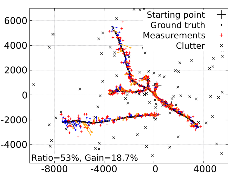
(a) PHD filter with no repulsion

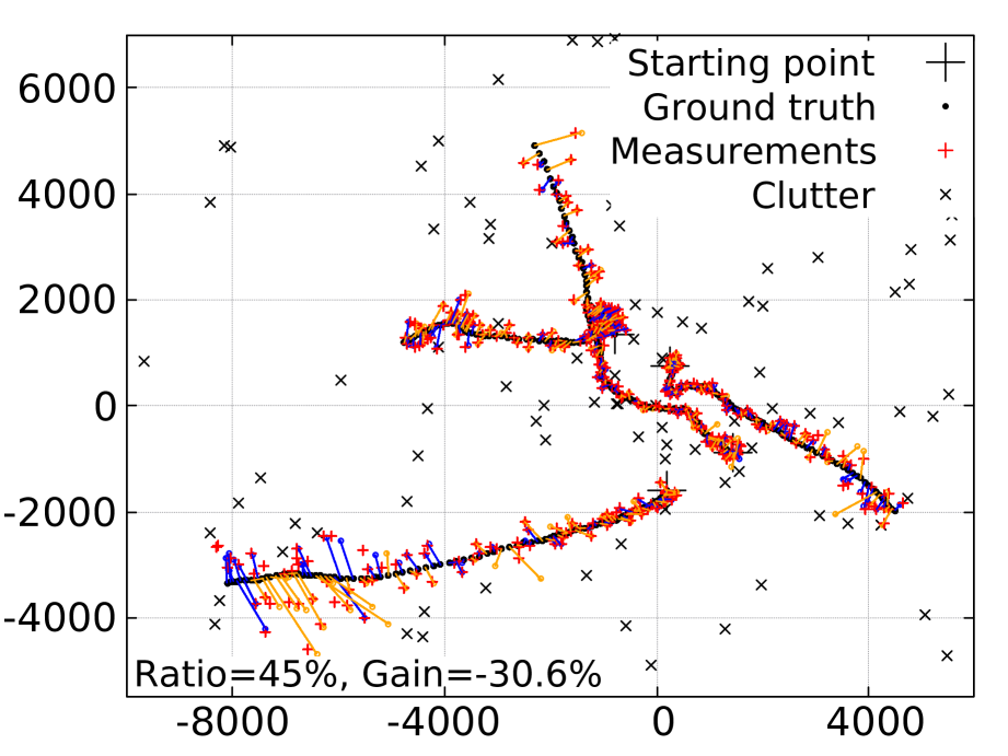
(b) PHD filter with repulsion

Figure 1: PHD filter simulations with and without repulsion

Figure 1-(1(b)) shows that when using a nonzero value for the repulsion parameter $\zeta=\zeta_{x}=\zeta_{y}$, the good estimate ratio with repulsive interaction becomes lower as compared with the non repulsive setting of Figure 1-(1(a)), with $50$ time steps. In Figure 1 the Poisson clutter rate is $l_{c}=1$, the probability of detection $p_{d}=0.9$ and the probability of survival is $p_{s}=1$, with four targets.

In Figures 2-(2(a))-(2(b)) we provide further illustrations of three-target interaction and PHD filter output of a single trial at different repulsion values $\zeta=0$ and $30$, with $15$ time steps and $p_{d}=p_{s}=1$.

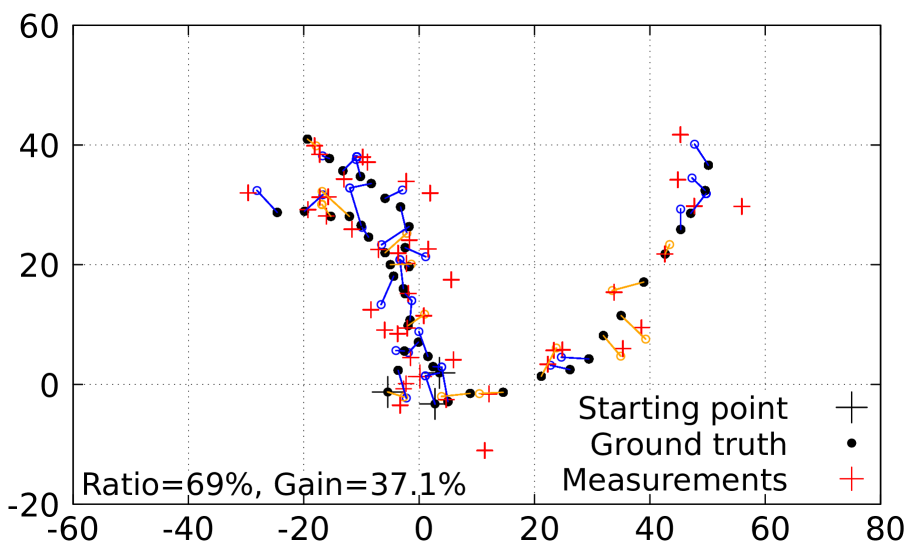
(a) PHD filter with data association for $\zeta=0$.

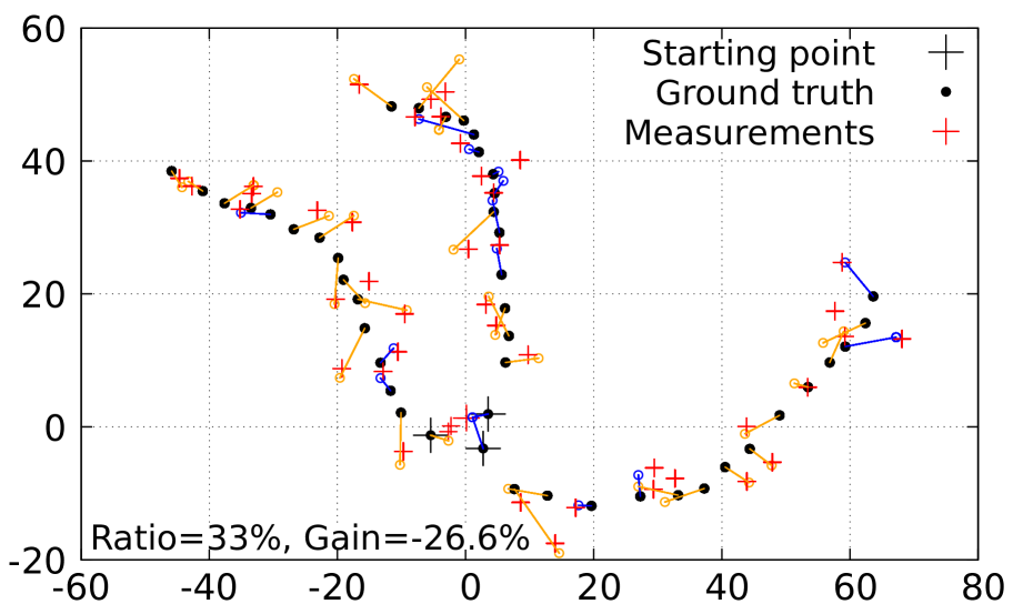
(b) PHD filter with data association for $\zeta=30$.

Figure 2: PHD filter with data association for $\zeta=0$ and $\zeta=30$.

Figure 2-(2(a)) shows the PHD filter output with $\zeta=0$, where the targets can become closer to each other without repulsion, and with positive gain. For the repulsion value $\zeta=30$ as in Figure 2-(2(b)) the repulsion effect among the three targets become much more evident, the good estimate ratio becomes lower, and the gain becomes negative.

The above results are summarized in Figure 3. Figure 3-(3(a)) presents the SMC-PHD filter first-order moment output with $200$ Monte Carlo runs and $10$ targets across $20$ time steps, with different repulsion parameter values $\zeta=0,4,8$. Figure 3-(3(b)) presents the good estimate ratio for various values of the repulsion coefficient $\zeta$, with $100$ Monte Carlo runs on three targets across $15$ time steps, with $p_{d}=1$ and no clutter.

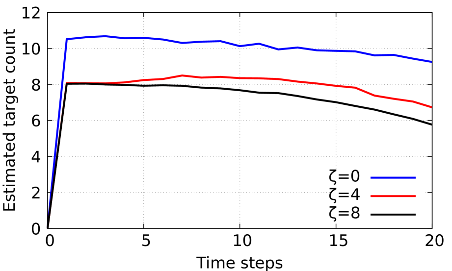
(a) First moment estimation of target count.

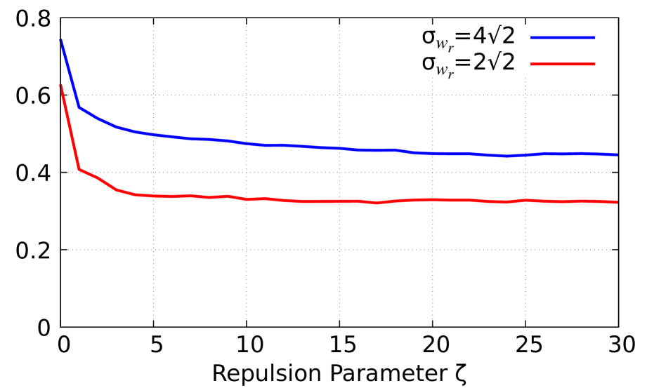
(b) Good estimate ratio with $p_{d}=1$ and no clutter.

Figure 3: Graphs of first moment target counts and good estimate ratios.

We note that the PHD filter is correctly estimating the target count when the repulsion coefficient $\zeta$ vanishes; however, the estimation falls short for nonzero values of $\zeta$, showing the performance degradation of the PPP-PHD filter in the presence of target interaction.

7 Determinantal PHD filtering algorithm

Initialization $(t=0)$

The state dynamics of the initial set of $N_{\Phi,0}$ particles is sampled according to a uniform distribution on the state space $\Lambda$. The diagonal entries of the prior discretized determinantal kernel $K_{\Phi,0}$ at time $t=0$ are initialized to $\gamma_{\Phi,0}/N_{\Phi,0}$ with $\gamma_{\Phi,0}$ a prior intensity value. The nondiagonal entries are initialized to $\alpha\gamma_{\Phi,0}/N_{\Phi,0}$ where $\alpha\geq 0$, except for those which are set to zero according to Condition (5.1) with the matrix index threshold $\eta=10\%$.

Using (4.7) we then compute the discretized Janossy kernel $J_{\Phi,0}$ which is needed for the evaluation of the posterior determinantal kernel $\tilde{K}_{\Phi|\Xi,0}$. Letting $P_{p}$ denote the number of resampled particles per target and $\gamma_{0}:=\sum_{i=1}^{N_{\Phi,0}}K_{\Phi|\Xi,0}(\mathbf{x}_{i},\mathbf{x}_{i})$, we resample $\tilde{N}_{0}:=P_{p}\times\lfloor\gamma_{0}\rfloor$ particles $\{\mathbf{x}_{i}\}_{i=1}^{\tilde{N}_{0}}$ that better describe the target locations as in Li et al. (2013) by maximizing the diagonal entries of $\tilde{K}_{\Phi|\Xi,0}$ over $\Lambda$, where $\lfloor\cdot\rfloor$ denotes the integer floor function. Those particles are then used to initialize the post-resampling determinantal kernel $K_{0}$ and to compute the post-resampling Janossy kernel $J_{0}$ in order to estimate the updated kernel $\tilde{K}_{\Phi|\Xi}$ from (5.5), (5.7) and (2). The updated kernel $\tilde{K}_{\Phi|\Xi}$ is then set as the prior kernel $K_{\Psi}$ of the next time step.

Initialization (time $t=0$)

  Set $\gamma_{\Phi,0}\in\mathbb{R}^{+}$, $P_{p}\in\mathbb{N}$, $\eta\in(0,1)$, and $\alpha\in\mathbb{R}^{+}$.

  Sample $N_{\Phi,0}$ particle state dynamics $\{\mathbf{x}_{i}\}_{i=1}^{N_{\Phi,0}}$ for initial birth process $\Phi$ uniformly distributed within state space $\Lambda$.

  Initialize the (prior) determinantal kernel $K_{\Phi,0}$.

  for $1\leq i,j\leq N_{\Phi,0}$ do

     $K_{\Phi,0}(\mathbf{x}_{i},\mathbf{x}_{i}):=$ $\gamma_{\Phi,0}/N_{\Phi,0}$

     if $i\neq j$ and $|i-j|\leq\eta P_{b}$ then

        $K_{\Phi,0}(\mathbf{x}_{i},\mathbf{x}_{j}):=$ $\alpha\gamma_{\Phi,0}/N_{\Phi,0}$

     end if

  end for

  Compute the Janossy kernel $J_{\Phi,0}:=(I-K_{\Phi,0})^{-1}K_{\Phi,0}$.

  Compute the posterior determinantal kernel $K_{\Phi|\Xi,0}$ using (5.5), (5.7) and (2).

  Perform resampling as in Li et al. (2013) to obtain the particle state dynamics $\{\mathbf{x}_{i}\}_{i=1}^{\tilde{N}_{0}}$ where $\tilde{N}_{0}:=P_{p}\times\lfloor\gamma_{0}\rfloor$ and $\gamma_{0}:=\sum_{i=1}^{N_{\Phi,0}}K_{\Phi|\Xi,0}(\mathbf{x}_{i},\mathbf{x}_{i})$.

  Initialize the post-resampling determinantal kernel $K_{0}$ as follows:

  for $1\leq i,j\leq\tilde{N}_{0}$ do

     $K_{0}(\mathbf{x}_{i},\mathbf{x}_{i}):=\gamma_{0}/\tilde{N}_{0}$

     if $i\neq j$ and $|i-j|\leq\eta P_{p}$ then

        $K_{0}(\mathbf{x}_{i},\mathbf{x}_{j}):=\alpha\gamma_{0}/\tilde{N}_{0}$

     end if

  end for

  Compute the post-resampling Janossy kernel $J_{0}=(I-K_{0})^{-1}K_{0}$.

  Compute the posterior determinantal kernel $\tilde{K}_{\Phi|\Xi,0}$ using (5.5), (5.7) and (2).

  Estimate the number of targets as $\gamma_{\Phi|\Xi,0}:=\sum_{i=1}^{\tilde{N}_{0}}\tilde{K}_{\Phi|\Xi,0}(\mathbf{x}_{i},\mathbf{x}_{i})$.

Algorithm $(t\geq 1)$

The general algorithm proceeds to compute the prediction state transition dynamics $\{\mathbf{x}_{t+1|t}^{(i)}\}_{i=1}^{\tilde{N}_{t}}$ using (6.1), followed by the computation of the prediction determinantal state transition kernel $K_{\Phi,t+1|t}$ using (5.3) and (5.4). Letting $P_{b}$ denote the number of particles per birth target and $\gamma_{\Phi,t+1}:=\sum_{i=1}^{\tilde{N}_{t}}K_{\Psi,t+1}(\mathbf{x}_{i},\mathbf{x}_{i})\nu(\{x_{i}\})$, we sample the state dynamics of $N_{\Phi,t+1}:=P_{b}\times\lfloor\gamma_{\Phi,t+1}\rfloor$ particles for the target birth process $\Phi$. The discretized prediction determinantal kernel $K_{\Phi,t+1|t}$ is then extended to incorporate the set of additional $N_{\Phi,t+1}$ particles by assigning the diagonal entries corresponding to these new particles to $\gamma_{\Phi,t+1}/N_{\Phi,t+1}$ and the nondiagonal entries to $\alpha\gamma_{\Phi,t+1}/N_{\Phi,t+1}$, and by setting all other new entries to $0$ according to Condition (5.1) with the matrix index threshold $\eta:=10\%$. Thereafter, we compute the discretized Janossy kernel $J_{\Phi,t+1|t}$ using (4.7) and then the discretized posterior determinantal kernel $K_{\Phi|\Xi,t+1}$ using (5.5), (5.7) and (2). Next, letting $\gamma_{t+1}:=\sum_{i=1}^{N_{t+1}}K_{\Phi|\Xi,t+1}(\mathbf{x}_{i},\mathbf{x}_{i})$ we resample $\tilde{N}_{t+1}:=P_{p}\times\lfloor\gamma_{t+1}\rfloor$ particles with state dynamics $\{\mathbf{x}_{i}\}_{i=1}^{\tilde{N}_{t+1}}$ as in Li et al. (2013), by maximizing the diagonal entries of $K_{\Phi|\Xi,t+1}$ over $\Lambda$. Those particles are then used to initialize the post-resampling determinantal kernel $K_{t+1}$ by setting diagonal entries to $\gamma_{t+1}/\tilde{N}_{t+1}$ and nondiagonal entries to $\alpha\gamma_{t+1}/\tilde{N}_{t+1}$, except for those which are set to zero according to Condition (5.1) with $\eta=10\%$. Finally, we recompute the post-resampling Janossy kernel $J_{t+1}$ and the posterior determinantal kernel $\tilde{K}_{\Phi|\Xi,t+1}$ using (5.5), (5.7) and (2).

DPP-PHD Filter (time $t+1\geq 1$)

  Compute the (prediction) state transition dynamics $\{\mathbf{x}_{t+1|t}^{(i)}\}_{i=1}^{\tilde{N}_{t}}$ from $\{\mathbf{x}_{t}^{(i)}\}_{i=1}^{\tilde{N}_{t}}$ based on (6.1).

  Compute the (prediction) determinantal state transition kernel $K_{\Phi,t+1|t}$ from $K_{\Psi,t+1}:=\tilde{K}_{\Phi|\Xi,t}$ using (5.3) and (5.4).

  Sample $N_{\Phi,t+1}$ new particle state dynamics for birth process $\Phi$ at time $t+1$ uniformly distributed within state space $\Lambda$ to generate $\{\mathbf{x}^{(i)}\}_{i=1}^{N_{\Phi,t+1}}$ where $N_{\Phi,t+1}:=P_{b}\times\lfloor\gamma_{\Phi,t+1}\rfloor$ and $\gamma_{\Phi,t+1}:=\sum_{i=1}^{\tilde{N}_{t}}K_{\Psi,t+1}(\mathbf{x}_{i},\mathbf{x}_{i})$.

  Extend the (prediction) determinantal kernel $K_{\Phi,t+1|t}$ to dimension $N_{t+1}:=\tilde{N}_{t}+N_{\Phi,t+1}$ with state dynamics $\{\mathbf{x}_{i}\}_{i=1}^{N_{t+1}}:=\{\mathbf{x}_{t+1|t}^{(i)}\}_{i=1}^{\tilde{N}_{t}}\cup\{\mathbf{x}^{(i)}\}_{i=1}^{N_{\Phi,t+1}}$, where the following indexes are allocated to new particles.

  for $\tilde{N}_{t}+1\leq i,j\leq N_{t+1}$ do

     $K_{\Phi,t+1|t}(\mathbf{x}_{i},\mathbf{x}_{i}):=\gamma_{\Phi,t+1}/N_{\Phi,t+1}$

     if $i\neq j$ and $|i-j|\leq\eta P_{b}$ then

        $K_{\Phi,t+1|t}(\mathbf{x}_{i},\mathbf{x}_{j}):=\alpha\gamma_{\Phi,t+1}/N_{\Phi,t+1}$

     end if

  end for

  for $1\leq i,j\leq N_{t+1}$ do

     if $i\leq\tilde{N}_{t}\And j\geq\tilde{N}_{t}+1$ then

        $K_{\Phi,t+1|t}(\mathbf{x}_{i},\mathbf{x}_{j}):=0$

        $K_{\Phi,t+1|t}(\mathbf{x}_{j},\mathbf{x}_{i}):=0$

     end if

  end for

  Compute the Janossy kernel $J_{\Phi,t+1|t}:=$ $(I-K_{\Phi,t+1|t})^{-1}{K_{\Phi,t+1|t}}$.

  Compute the posterior determinantal kernel $K_{\Phi|\Xi,t+1}$ using (5.5), (5.7) and (2).

  Perform resampling as in Li et al. (2013) to obtain the particle state dynamics $\{\mathbf{x}_{i}\}_{i=1}^{\tilde{N}_{t+1}}$ where $\tilde{N}_{t+1}:=P_{p}\times\lfloor\gamma_{t+1}\rfloor$ (capped at $1000$ particles) and $\gamma_{t+1}:=\sum_{i=1}^{N_{t+1}}K_{\Phi|\Xi,t+1}(\mathbf{x}_{i},\mathbf{x}_{i})$.

  Initialize the post-resampling determinantal kernel $K_{t+1}$ by

  for $1\leq i,j\leq\tilde{N}_{t+1}$ do

     $K_{t+1}(\mathbf{x}_{i},\mathbf{x}_{i}):=\gamma_{t+1}/\tilde{N}_{t+1}$

     if $i\neq j$ and $|i-j|\leq\eta P_{p}$ then

        $K_{t+1}(\mathbf{x}_{i},\mathbf{x}_{j}):=$ $\alpha\gamma_{t+1}/\tilde{N}_{t+1}$

     end if

  end for

  Compute the post-resampling Janossy kernel $J_{t+1}=(I-K_{t+1})^{-1}{K_{t+1}}.$

  Compute the posterior determinantal kernel $\tilde{K}_{\Phi|\Xi,t+1}$ using (5.5), (5.7) and (2).

  Estimate the number of targets as $\gamma_{\Phi|\Xi,t+1}:=$ $\sum_{i=1}^{\tilde{N}_{t+1}}\tilde{K}_{\Phi|\Xi,t+1}(\mathbf{x}_{i},\mathbf{x}_{i})$.

The complexity of this DPP-PHD filter is cubic in the number of discretization steps due to the presence of matrix inversions in the algorithm.

Numerical results

In Figure 4 we assess the spooky effect (see Fränken et al. (2009)) of our DPP-PHD filter, following the approach applied in Schlangen et al. (2018) to second-order PHD filters. Our tracking scenario consists of two disjoint square domains $A$ and $B$ of size $150$ m by $150$ m, which are located 150m diagonally apart. In each domain, $10$ targets are initialized and their state dynamics are centrally distributed at the first time step. The runtime of the experiment is set at $50$ with $100$ Monte Carlo (MC) runs, the targets survive throughout ($p_{s}=1$), and their trajectories remain within the observation domains. In Figure 4 we take the spatial standard deviations (s.d.) $\sigma_{v_{x}}=\sigma_{v_{y}}=1.0$ m/s², turn-rate noise s.d. $\sigma_{v_{\theta}}=\pi=180$ rad/s, bearing distribution s.d. $\sigma_{w_{\omega}}=\pi=180$ rad, and range distribution s.d. $\sigma_{w_{r}}=\sqrt{2}$ m.

In a similar setting to Schlangen et al. (2018), all targets in domain $B$ are compelled to be misdetected in every cycle of $10$ time steps. We use a constant probability of detection $p_{d}=0.9$ and mean clutter count at $5$ in each measurement space.

At initialization in Figure 4 we set $N_{\Phi,0}=800$, $\gamma_{\Phi,0}=2$ and $\alpha=4$. The DPP-PHD filter implementation uses $P_{p}=30$ resampled particles per target, and $P_{b}=10$ particles per birth target.

Figure 4-(4(a)) shows the estimated intensities in domains $A$ and $B$, where domain $A$ is unaffected by the rapid drop in the intensity of domain $B$. The posterior correlation estimates in Figure 4-(4(b)) are computed by rescaling the covariance expression (4.6) written as

$$c^{(2)}_{\Phi\mid\Xi=z_{1:m}}(A,B)=-\int_{A\times B}(K_{\Phi\mid\Xi=z_{1:m}}(x,y))^{2}\nu(dx)\nu(dy),$$

as in Corollary A.4, where $K_{\Phi\mid\Xi=z_{1:m}}(x,y)$ is estimated as in Proposition A.3 from (5.5) and (5.7). Figure 4-(4(b)) shows negative correlations due to the determinantal point process nature, which leads to a drop in negative correlation during the compelled misdetection at each $10$-steps cycle.

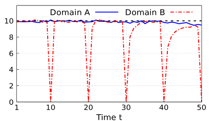
(a) Target counts estimates.

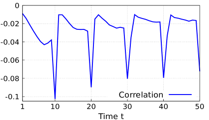
(b) Correlation estimates.

Figure 4: MC estimates with $p_{d}=0.9$ and $5$ clutter points per domain with $\alpha=4.0$.

Figure 5 presents miss-distance performance estimates for the experiment of Figure 4, using the $L^{2}$-Optimal Mass Transfer (OMAT, Hoffman and Mahler (2004)) metric, and the $L^{2}$-Optimal Subpattern Assignment (OSPA, Schumacher et al. (2008)) metric with threshould $c=100$, which solves the inconsistencies encountered with the OMAT metric and takes into account differences in cardinalities.

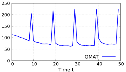
(a) OMAT distance estimates.

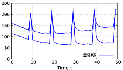
(b) OSPA distance estimates.

Figure 5: Miss-distance performance evaluation.

In Figure 6 we compare the robustness of the DPP and PPP-PHD filters when both filters are subjected to sudden death in the number of targets in a single domain of size $100$m by $100$m, beginning with $15$ targets at the first time step.

Figure 6-(6(a)) uses $300$ Monte Carlo runs, while Figure 6-(6(b)) relies on $200$ Monte Carlo runs. The runtime of each Monte Carlo run spans from time $t=0$ to time $t=15$, and the probability of survival is $p_{s}:=1$. The initial $15$ targets are maintained until time $t=9$ when $10$ random targets are forced to die and the remaining $5$ targets survive until the end of the time interval. In Figure 6 we take the spatial standard deviations (s.d.) $\sigma_{v_{x}}=\sigma_{v_{y}}=1.0$ m/s², turn-rate noise s.d. $\sigma_{v_{\theta}}=\pi=180$ rad/s, with bearing and range distribution s.d. $\sigma_{w_{\omega}}=\pi=180$ rad, $\sigma_{w_{r}}=\sqrt{2}$ m as in Figure 4, with probability of detection $p_{d}=0.95$, mean clutter count at $1$ up to time $t=9$ and then at $0.06$ afterwards for Figure 6-(6(b)), and mean clutter count at $1$ up to time $t=9$ and then at $0.3$ afterwards for Figure 6-(6(a)). At initialization in Figure 6, we set $N_{\Phi,0}=6000$ and $\gamma_{\Phi,0}=0.2$. Both our DPP and PPP-PHD filter implementations use $P_{p}=50$ resampled particles per target in Figure 6, $P_{b}=60$ particles per birth target in Figure 6-(6(b)), and $P_{b}=40$ particles per birth target in Figure 6-(6(a)).

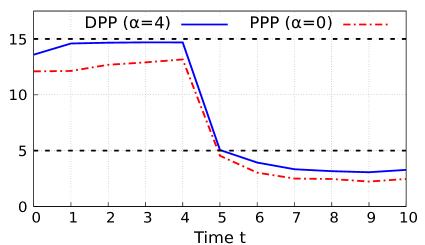
(a) Graph with $P_{p}=50$ and $P_{b}=40$.

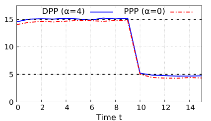
(b) Graph with $P_{p}=50$ and $P_{b}=60$.

Figure 6: Target count estimates from $15$ to $5$ targets, $p_{d}=0.9$ and $1$ to $0.3$ clutter points.

In Figure 7 we compare the robustness and performance recovery of the DPP and PPP-PHD filters when subjected to a rapid birth in the number of targets in a single domain of size $100$ m by $100$ m. The experiment starts with a single target which survives throughout the $45$ time steps, without birth of new targets from time $t=0$ to time $t=9$. At time $t=10$, $9$ new targets are born centrally distributed within the target space and survive through the remaining time steps.

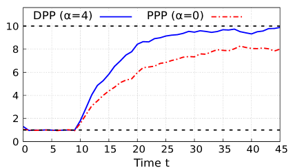
(a) Graph with $P_{p}=40$ and $P_{b}=9$.

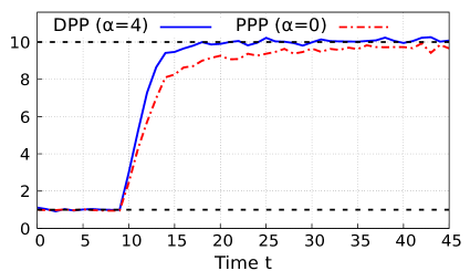
(b) Graph with $P_{p}=50$ and $P_{b}=15$.

Figure 7: Target count estimates from $0$ to $10$ targets, $p_{d}=0.9$ and $0$ to $5$ clutter points.

Each Monte Carlo run spans $45$ time steps, with $400$ and $100$ Monte Carlo runs in the experiments of Figures 7-(7(a)) and 7-(7(b)) respectively. In Figure 7 the spatial standard deviations (s.d.) $\sigma_{v_{x}}=\sigma_{v_{y}}=1.0$ m/s², turn-rate noise s.d. $\sigma_{v_{\theta}}=\pi=180$ rad/s, and bearing and range s.d. $\sigma_{w_{\omega}}=\pi=180$ rad, $\sigma_{w_{r}}=\sqrt{2}$ m are the same as in Figure 6. The model generates measurement information from each target with a constant probability of detection $p_{d}=0.90$, mean clutter count at $0$ up to time $t=9$ and then at $5$ afterwards for Figure 7-(7(a)), and mean clutter count at $0.05$ up to time $t=9$ and then at $5$ afterwards for Figure 7-(7(b)). We set $N_{\Phi,0}=300$ and $\gamma_{\Phi,0}=0.2$ at initialization in Figure 7. Both DPP and PPP-PHD filter implementations use $P_{b}=40$ and $P_{b}=50$ resampled particles per target in Figure 7-(7(a)) and Figure 7-(7(b)) respectively. For the target birth process we set $P_{b}=9$ and $P_{b}=15$ particles per birth target in Figure 7-(7(a)) and Figure 7-(7(b)) respectively.

Appendix A Appendix - Janossy density approximation

Since the corrector terms $l^{(1)}_{z_{1:m}}(x)$, $l^{(1)}_{z_{1:m}}(x;z)$, $l^{(2)}_{z_{1:m}}(x,y)$, $l^{(2)}_{z_{1:m}}(x,y;z)$, $l^{(2)}_{z_{1:m}}(x,y;z,z^{\prime})$ in (3.15), (3.19) and the kernel update formula (2) have no closed form expression in the determinantal setting, we propose to use the Janossy density approximations

$$j^{(n)}_{\Phi}(x_{1},\ldots,x_{r-1},x,x_{r+1},\ldots,x_{n})\simeq J_{\Phi}(x,x)j^{(n-1)}_{\Phi}(x_{1},\ldots,x_{r-1},x_{r+1},\ldots,x_{n})$$ (A.1)

$n\geq 1$, which corresponds to a (Poisson) first-order approximation, and

$$j^{(n)}_{\Phi}(x_{1},\ldots,x_{r-1},x,x_{r+1},\ldots,x_{p-1},y,x_{p+1},\ldots,x_{n})$$

$$\simeq (J_{\Phi}(x,x)J_{\Phi}(y,y)-(J_{\Phi}(x,y))^{2})j^{(n-2)}_{\Phi}(x_{1},\ldots,\hat{x}_{r},\ldots,\hat{x}_{p},\ldots,x_{n}),$$

$n\geq 2$, which corresponds to a second-order (determinant) approximation, obtained from (4.8) by assuming that the off-diagonal entries $J_{\Phi}(x_{i},x_{j})$, $i\not=j$, are small.

This Janossy approximation is specially relevant to $\alpha$-determinantal Ginibre point processes (GPP) which approximate a Poisson point process when $\alpha\in[-1,0)$ tends to $0$, see Shirai and Takahashi (2003).

Proposition A.1

Under (A.1) we have the first-order Poisson approximations $l^{(1)}_{z_{1:m}}(x)\simeq J_{\Phi}(x,x)$, $m\geq 0$, and

$$l^{(1)}_{z_{1:m}}(x;z)\simeq\frac{J_{\Phi}(x,x)}{l_{c}(z)+\int_{\Lambda}J_{\Phi}(u,u)\tilde{l}_{d}(z|u)\nu(du)},$$

$z\in z_{1:m}$, $x\in\Lambda$, $m\geq 1$.

Proof. By (3.16) and (A.1) we have

$$\Upsilon^{(1)}_{z_{1:m}}(x) = \displaystyle\sum_{S\subset\{1,\ldots,m\}}\sum_{p\geq|S|}\frac{q_{d}^{p-|S|}}{(p-|S|)!}\prod_{j\notin S}l_{c}(z_{j})\int_{\Lambda^{p}}j^{(p+1)}_{\Phi}(x_{1:p},x)\prod_{i\in S}\tilde{l}_{d}(z_{i}|x_{i})\nu(dx_{1:p})$$ (A.3)

$$\simeq J_{\Phi}(x,x)\sum_{p\geq 0}\displaystyle\sum_{S\subset\{1,\ldots,m\}\atop|S|\leq p}\frac{q_{d}^{p-|S|}}{(p-|S|)!}\prod_{j\notin S}l_{c}(z_{j})\int_{\Lambda^{p}}j^{(p)}_{\Phi}(x_{1:p})\prod_{i\in S}\tilde{l}_{d}(z_{i}|x_{i})\nu(dx_{1:p})$$

$$= J_{\Phi}(x,x)j^{(m)}_{\Xi}(z_{1},\ldots,z_{m}),$$

by (3.9), which yields the approximation $l^{(1)}_{z_{1:m}}(x)\simeq J_{\Phi}(x,x)$. On the other hand, for $r=1,\ldots,m$, using again (A.1) and (3.9) we have

$$j^{(m)}_{\Xi}(z_{1},\ldots,z_{m})=\displaystyle\frac{\partial_{\delta_{z_{1}}}}{\partial g}\cdots\frac{\partial_{\delta_{z_{m}}}}{\partial g}{\cal G}_{\Phi,\Xi}({\bf 1},g)_{\mid g=0}$$

$$=\displaystyle\sum_{p\geq 0}\sum_{S\subset\{1,\ldots,m\}\atop|S|\leq p}\frac{q_{d}^{p-|S|}}{(p-|S|)!}\prod_{j\notin S}l_{c}(z_{j})\int_{\Lambda^{p}}j^{(p)}_{\Phi}(y_{1:p})\prod_{i\in S}\tilde{l}_{d}(z_{i}|y_{i})\nu(dy_{1:p})$$

$$\simeq l_{c}(z_{r})\sum_{p\geq 0}\displaystyle\sum_{S\subset\{1,\ldots,m\}\setminus\{r\}\atop|S|\leq p}\frac{q_{d}^{p-|S|}}{(p-|S|)!}\prod_{j\notin S}l_{c}(z_{j})\int_{\Lambda^{p}}j^{(p)}_{\Phi}(x_{1:p})\prod_{i\in S}\tilde{l}_{d}(z_{i}|x_{i})\nu(dx_{1:p})$$

$$\quad+\int_{\Lambda}J_{\Phi}(x_{r},x_{r})\tilde{l}_{d}(z_{r}|x_{r})\nu(dx_{r})\sum_{p\geq 0}\displaystyle\sum_{S\subset\{1,\ldots,m\}\atop|S|\leq p+1,r\in S}\frac{q_{d}^{p+1-|S|}}{(p+1-|S|)!}\prod_{j\notin S}l_{c}(z_{j})\int_{\Lambda^{p}}j^{(p)}_{\Phi}(x_{1:p})\prod_{i\in S\setminus\{r\}}\tilde{l}_{d}(z_{i}|x_{i})\nu(dx_{1:p})$$

$$=l_{c}(z_{r})\sum_{p\geq 0}\displaystyle\sum_{S\subset\{1,\ldots,m\}\setminus\{r\}\atop|S|\leq p}\frac{q_{d}^{p-|S|}}{(p-|S|)!}\prod_{j\notin S}l_{c}(z_{j})\int_{\Lambda^{p}}j^{(p)}_{\Phi}(x_{1:p})\prod_{i\in S}\tilde{l}_{d}(z_{i}|x_{i})\nu(dx_{1:p})$$

$$\quad+\int_{\Lambda}J_{\Phi}(u,u)\tilde{l}_{d}(z_{r}|u)\nu(du)\sum_{p\geq 0}\displaystyle\sum_{S\subset\{1,\ldots,m\}\setminus\{r\}\atop|S|\leq p}\frac{q_{d}^{p-|S|}}{(p-|S|)!}\prod_{j\notin S}l_{c}(z_{j})\int_{\Lambda^{p}}j^{(p)}_{\Phi}(x_{1:p})\prod_{i\in S\setminus\{r\}}\tilde{l}_{d}(z_{i}|x_{i})\nu(dx_{1:p})$$

$$=\left(l_{c}(z_{r})+\int_{\Lambda}J_{\Phi}(u,u)\tilde{l}_{d}(z_{r}|u)\nu(du)\right)\sum_{p\geq 0}\displaystyle\sum_{S\subset\{1,\ldots,m\}\setminus\{r\}\atop|S|\leq p}\frac{q_{d}^{p-|S|}}{(p-|S|)!}\prod_{j\notin S}l_{c}(z_{j})\int_{\Lambda^{p}}j^{(p)}_{\Phi}(x_{1:p})\prod_{i\in S}\tilde{l}_{d}(z_{i}|x_{i})\nu(dx_{1:p})$$

$$=\left(l_{c}(z_{r})+\int_{\Lambda}J_{\Phi}(u,u)\tilde{l}_{d}(z_{r}|u)\nu(du)\right)j^{(m-1)}_{\Xi}(z_{1},\ldots,z_{r-1},z_{r+1},\ldots,z_{m}).$$ (A.4)

We conclude by taking $z_{r}=z$ and noting that by (3.15) and (A.3)-(A.4) we have

$$l^{(1)}_{z_{1:m}}(x;z)=\frac{\Upsilon^{(1)}_{z_{1:m}\!\setminus z}(x)}{j^{(m)}_{\Xi}(z_{1:m})}\simeq J_{\Phi}(x,x)\frac{j^{(m-1)}_{\Xi}(z_{1:m}\!\setminus z)}{j^{(m)}_{\Xi}(z_{1:m})}.$$

$\square$

Proposition A.2

Under (A.1)-(A) we have the second-order approximations

$$l^{(2)}_{z_{1:m}}(x,y)\simeq J_{\Phi}(x,x)J_{\Phi}(y,y)-J_{\Phi}(x,y)^{2},\quad l^{(2)}_{z_{1:m}}(x,y;z)\simeq\frac{J_{\Phi}(x,x)J_{\Phi}(y,y)-J_{\Phi}(x,y)^{2}}{l_{c}(z)+\int_{\Lambda}J_{\Phi}(u,u)\tilde{l}_{d}(z|u)\nu(du)},$$

$z\in z_{1:m}$, $x,y\in\Lambda$, $m\geq 1$, and

$$l^{(2)}_{z_{1:m}}(x,y;z,z^{\prime})\simeq\frac{J_{\Phi}(x,x)J_{\Phi}(y,y)-J_{\Phi}(x,y)^{2}}{s_{c}(z)s_{c}(z^{\prime})-\int_{\Lambda^{2}}J_{\Phi}(u,v)^{2}\tilde{l}_{d}(z|u)\tilde{l}_{d}(z^{\prime}|v)\nu(du)\nu(dv)},$$

$z,z^{\prime}\in z_{1:m}$, $z\not=z^{\prime}$, $x,y\in\Lambda$, $m\geq 2$, where

$$s_{c}(z):=l_{c}(z)+\int_{\Lambda}J_{\Phi}(v,v)\tilde{l}_{d}(z|v)\nu(dv),\qquad z\in\Lambda.$$ (A.5)

Proof. By (3.21) and (A) we have

$$\Upsilon^{(2)}_{z_{1:m}}(x,y)=\sum_{p\geq 0}\displaystyle\sum_{S\subset\{1,\ldots,m\}\atop|S|\leq p}\frac{q_{d}^{p-|S|}}{(p-|S|)!}\prod_{j\notin S}l_{c}(z_{j})\int_{\Lambda^{p}}j^{(p+2)}_{\Phi}(x_{1:p},x,y)\prod_{i\in S}\tilde{l}_{d}(z_{i}|x_{i})\nu(dx_{1:p})$$

$$=(J_{\Phi}(x,x)J_{\Phi}(y,y)-J_{\Phi}(x,y)^{2})\sum_{p\geq 0}\displaystyle\sum_{S\subset\{1,\ldots,m\}\atop|S|\leq p}\frac{q_{d}^{p-|S|}}{(p-|S|)!}\prod_{j\notin S}l_{c}(z_{j})\int_{\Lambda^{p}}j^{(p)}_{\Phi}(x_{1:p})\prod_{i\in S}\tilde{l}_{d}(z_{i}|x_{i})\nu(dx_{1:p})$$

$$=(J_{\Phi}(x,x)J_{\Phi}(y,y)-J_{\Phi}(x,y)^{2})j^{(m)}_{\Xi}(z_{1:m}),$$ (A.6)

and for $r,u=1,\ldots,m$, using (A.1)-(A) and (3.9) we find

$$j^{(m)}_{\Xi}(z_{1:m})=\displaystyle\sum_{n\geq 0}\sum_{S\subset\{1,\ldots,m\}\atop|S|\leq n}\prod_{j\notin S}l_{c}(z_{j})\frac{q_{d}^{n-|S|}}{(n-|S|)!}\int_{\Lambda^{n}}j^{(n)}_{\Phi}(y_{1:n})\prod_{i\in S}\tilde{l}_{d}(z_{i}|y_{i})\nu(dy_{1:n})$$

$$\simeq l_{c}(z_{r})l_{c}(z_{u})\sum_{p\geq 0}\displaystyle\sum_{S\subset\{1,\ldots,m\}\setminus\{r,u\}\atop|S|\leq p}\frac{q_{d}^{p-|S|}}{(p-|S|)!}\prod_{j\notin S}l_{c}(z_{j})\int_{\Lambda^{p}}j^{(p)}_{\Phi}(x_{1:p})\prod_{i\in S}\tilde{l}_{d}(z_{i}|x_{i})\nu(dx_{1:p})$$

$$\quad+l_{c}(z_{r})\int_{\Lambda}J_{\Phi}(v,v)\tilde{l}_{d}(z_{u}|v)\nu(dv)$$

$$\qquad\times\sum_{p\geq 0}\int_{\Lambda^{p}}\displaystyle\sum_{S\subset\{1,\ldots,m\}\setminus\{r\}\atop|S|\leq p+1,u\in S}\frac{q_{d}^{p+1-|S|}}{(p+1-|S|)!}j^{(p)}_{\Phi}(x_{1:p})\prod_{j\notin S}l_{c}(z_{j})\prod_{i\in S\setminus\{u\}}\tilde{l}_{d}(z_{i}|x_{i})\nu(dx_{1:p})$$

$$\quad+l_{c}(z_{u})\int_{\Lambda}J_{\Phi}(v,v)\tilde{l}_{d}(z_{r}|v)\nu(dv)$$

$$\qquad\times\sum_{p\geq 0}\int_{\Lambda^{p}}\displaystyle\sum_{S\subset\{1,\ldots,m\}\setminus\{u\}\atop|S|\leq p+1,r\in S}\frac{q_{d}^{p+1-|S|}}{(p+1-|S|)!}j^{(p)}_{\Phi}(x_{1:p})\prod_{j\notin S}l_{c}(z_{j})\prod_{i\in S\setminus\{r\}}\tilde{l}_{d}(z_{i}|x_{i})\nu(dx_{1:p})$$

$$\quad+\int_{\Lambda}(J_{\Phi}(x_{r},x_{r})J_{\Phi}(x_{u},x_{u})-J_{\Phi}(x_{r},x_{u})^{2})\tilde{l}_{d}(z_{r}|x_{r})\tilde{l}_{d}(z_{u}|x_{u})\nu(dx_{r})\nu(dx_{u})$$

$$\qquad\times\sum_{p\geq 0}\int_{\Lambda^{p}}\displaystyle\sum_{S\subset\{1,\ldots,m\}\atop|S|\leq p+2,r\in S}\frac{q_{d}^{p+2-|S|}}{(p+2-|S|)!}j^{(p)}_{\Phi}(x_{1:p})\prod_{j\notin S}l_{c}(z_{j})\prod_{i\in S\setminus\{r,u\}}\tilde{l}_{d}(z_{i}|x_{i})\nu(dx_{1:p})$$

$$=l_{c}(z_{r})l_{c}(z_{u})\sum_{p\geq 0}\int_{\Lambda^{p}}\displaystyle\sum_{S\subset\{1,\ldots,m\}\setminus\{r,u\}\atop|S|\leq p}\frac{q_{d}^{p-|S|}}{(p-|S|)!}j^{(p)}_{\Phi}(x_{1:p})\prod_{j\notin S}l_{c}(z_{j})\prod_{i\in S}\tilde{l}_{d}(z_{i}|x_{i})\nu(dx_{1:p})$$

$$\quad+l_{c}(z_{r})\int_{\Lambda}J_{\Phi}(v,v)\tilde{l}_{d}(z_{u}|v)\nu(dv)\sum_{p\geq 0}\int_{\Lambda^{p}}\displaystyle\sum_{S\subset\{1,\ldots,m\}\setminus\{r,u\}\atop|S|\leq p,u\in S}\frac{q_{d}^{p-|S|}}{(p-|S|)!}j^{(p)}_{\Phi}(x_{1:p})\prod_{j\notin S}l_{c}(z_{j})\prod_{i\in S}\tilde{l}_{d}(z_{i}|x_{i})\nu(dx_{1:p})$$

$$\quad+l_{c}(z_{u})\int_{\Lambda}J_{\Phi}(v,v)\tilde{l}_{d}(z_{r}|v)\nu(dv)\sum_{p\geq 0}\int_{\Lambda^{p}}\displaystyle\sum_{S\subset\{1,\ldots,m\}\setminus\{r,u\}\atop|S|\leq p,r\in S}\frac{q_{d}^{p-|S|}}{(p-|S|)!}j^{(p)}_{\Phi}(x_{1:p})\prod_{j\notin S}l_{c}(z_{j})\prod_{i\in S}\tilde{l}_{d}(z_{i}|x_{i})\nu(dx_{1:p})$$

$$\quad+\int_{\Lambda^{2}}(J_{\Phi}(u,u)J_{\Phi}(v,v)-J_{\Phi}(u,v)^{2})\tilde{l}_{d}(z_{r}|u)\tilde{l}_{d}(z_{u}|v)\nu(du)\nu(dv)$$

$$\qquad\times\sum_{p\geq 0}\int_{\Lambda^{p}}\sum_{S\subset\{1,\ldots,m\}\setminus\{r,u\}\atop|S|\leq p}\frac{q_{d}^{p-|S|}}{(p-|S|)!}j^{(p)}_{\Phi}(x_{1:p})\prod_{j\notin S}l_{c}(z_{j})\prod_{i\in S}\tilde{l}_{d}(z_{i}|x_{i})\nu(dx_{1:p})$$

$$=\left(l_{c}(z_{r})l_{c}(z_{u})+l_{c}(z_{r})\int_{\Lambda}J_{\Phi}(v,v)\tilde{l}_{d}(z_{u}|v)\nu(dv)+l_{c}(z_{u})\int_{\Lambda}J_{\Phi}(v,v)\tilde{l}_{d}(z_{r}|v)\nu(dv)\right.$$

$$\left.\quad+\int_{\Lambda^{2}}(J_{\Phi}(u,u)J_{\Phi}(v,v)-J_{\Phi}(u,v)^{2})\tilde{l}_{d}(z_{r}|u)\tilde{l}_{d}(z_{u}|v)\nu(du)\nu(dv)\right)$$

$$\qquad\times\sum_{p\geq 0}\int_{\Lambda^{p}}\displaystyle\sum_{S\subset\{1,\ldots,m\}\setminus\{r,u\}\atop|S|\leq p}\frac{q_{d}^{p-|S|}}{(p-|S|)!}j^{(p)}_{\Phi}(x_{1:p})\prod_{j\notin S}l_{c}(z_{j})\prod_{i\in S}\tilde{l}_{d}(z_{i}|x_{i})\nu(dx_{1:p})$$

$$=\left(l_{c}(z_{r})l_{c}(z_{u})+l_{c}(z_{r})\int_{\Lambda}J_{\Phi}(v,v)\tilde{l}_{d}(z_{u}|v)\nu(dv)\right.$$

$$\left.\quad+l_{c}(z_{u})\int_{\Lambda}J_{\Phi}(v,v)\tilde{l}_{d}(z_{r}|v)\nu(dv)+\int_{\Lambda^{2}}(J_{\Phi}(u,u)J_{\Phi}(v,v)-J_{\Phi}(u,v)^{2})\tilde{l}_{d}(z_{r}|u)\tilde{l}_{d}(z_{u}|v)\nu(du)\nu(dv)\right)$$

$$\qquad\times j^{(m-2)}_{\Xi}(z_{1},\ldots,z_{r-1},z_{r+1},\ldots,z_{u-1},z_{u+1},\ldots,z_{m})$$

$$\quad=\left(s_{c}(z_{r})s_{c}(z_{u})-\int_{\Lambda^{2}}J_{\Phi}(u,v)^{2}\tilde{l}_{d}(z_{r}|u)\tilde{l}_{d}(z_{u}|v)\nu(du)\nu(dv)\right)$$ (A.7)

$$\qquad\times j^{(m-2)}_{\Xi}(z_{1},\ldots,z_{r-1},z_{r+1},\ldots,z_{u-1},z_{u+1},\ldots,z_{m}).$$

We conclude by taking $(z_{r},z_{u})=(z,z^{\prime})$ and noting that by (3.20) and (A.6)-(A.7) we have

$$l^{(2)}_{z_{1:m}}(x,y,z,z^{\prime}) = \frac{\Upsilon^{(2)}_{z_{1:m}\!\setminus\{z,z^{\prime}\}}(x,y)}{j^{(m)}_{\Xi}(z_{1:m})}$$

$$\simeq (J_{\Phi}(x,x)J_{\Phi}(y,y)-J_{\Phi}(x,y)^{2})\frac{j^{(m-2)}_{\Xi}(z_{1:m}\!\setminus\{z,z^{\prime}\})}{j^{(m)}_{\Xi}(z_{1:m})}$$

$$\simeq \frac{(J_{\Phi}(x,x)J_{\Phi}(y,y)-J_{\Phi}(x,y)^{2})}{s_{c}(z)s_{c}(z^{\prime})-\int_{\Lambda^{2}}J_{\Phi}(u,v)^{2}\tilde{l}_{d}(z|u)\tilde{l}_{d}(z^{\prime}|v)\nu(du)\nu(dv)},$$

$z,z^{\prime}\in z_{1:m}$, $z\not=z^{\prime}$, $m\geq 2$. Similarly, by (3.19) and (A.4), (A.6) we also have

$$l^{(2)}_{z_{1:m}}(x,y;z) = \frac{\Upsilon^{(2)}_{z_{1:m}\!\setminus z}(x,y)}{j^{(m)}_{\Xi}(z_{1:m})}$$

$$\simeq (J_{\Phi}(x,x)J_{\Phi}(y,y)-J_{\Phi}(x,y)^{2})\frac{j^{(m-1)}_{\Xi}(z_{1:m}\!\setminus z)}{j^{(m)}_{\Xi}(z_{1:m})}$$

$$\simeq \frac{J_{\Phi}(x,x)J_{\Phi}(y,y)-J_{\Phi}(x,y)^{2}}{l_{c}(z)+\int_{\Lambda}J_{\Phi}(u,u)\tilde{l}_{d}(z|u)\nu(du)},\qquad z\in z_{1:m},\quad m\geq 1.$$

$\square$

As a consequence of (3.3) and Proposition A.2, the second-order conditional factorial moment density of $\Phi$ given that $\Xi=z_{1:m}=(z_{1},\ldots,z_{m})$ will be approximated as

$$\rho^{(2)}_{\Phi\mid\Xi=z_{1:m}}(x,y)\simeq q_{d}^{2}(J_{\Phi}(x,x)J_{\Phi}(y,y)-J_{\Phi}(x,y)^{2})$$

$$+q_{d}\sum_{z\in z_{1:m}}\frac{(J_{\Phi}(x,x)J_{\Phi}(y,y)-J_{\Phi}(x,y)^{2})\big{(}\tilde{l}_{d}(z|x)+\tilde{l}_{d}(z|y)\big{)}}{s_{c}(z)}$$

$$+\sum_{z,z^{\prime}\in z_{1:m}\atop z\not=z^{\prime}}\frac{(J_{\Phi}(x,x)J_{\Phi}(y,y)-J_{\Phi}(x,y)^{2})\tilde{l}_{d}(z|x)\tilde{l}_{d}(z^{\prime}|y)}{s_{c}(z)s_{c}(z^{\prime})-\int_{\Lambda^{2}}J_{\Phi}(u,v)^{2}\tilde{l}_{d}(z|u)\tilde{l}_{d}(z^{\prime}|v)\nu(du)\nu(dv)},$$

$m\geq 0$, with $\rho^{(2)}_{\Phi\mid\Xi=z_{1:m}}(x,x):=0$, $x\in\Lambda$.

Proposition A.3

The (approximate) kernel update formula is given by

$$K_{\Phi\mid\Xi=z_{1:m}}(x,y)^{2} \simeq q^{2}_{d}J_{\Phi}(x,y)^{2}+q_{d}J_{\Phi}(x,y)^{2}\sum_{z\in z_{1:m}}\frac{\big{(}\tilde{l}_{d}(z|x)+\tilde{l}_{d}(z|y)\big{)}}{s_{c}(z)}\displaystyle$$

$$\displaystyle+J_{\Phi}(x,x)J_{\Phi}(y,y)\sum_{z,z^{\prime}\in z_{1:m}}\frac{\tilde{l}_{d}(z|x)\tilde{l}_{d}(z^{\prime}|y)}{s_{c}(z)s_{c}(z^{\prime})}$$

$$+\sum_{z,z^{\prime}\in z_{1:m}\atop z\not=z^{\prime}}\frac{(J_{\Phi}(x,y)^{2}-J_{\Phi}(x,x)J_{\Phi}(y,y))\tilde{l}_{d}(z|x)\tilde{l}_{d}(z^{\prime}|y)}{s_{c}(z)s_{c}(z^{\prime})-\int_{\Lambda^{2}}J_{\Phi}(u,v)^{2}\tilde{l}_{d}(z|u)\tilde{l}_{d}(z^{\prime}|v)\nu(du)\nu(dv)},$$

$m\geq 0$, $x,y\in\Lambda$.

Proof. By (3.14) and Proposition A.1, we have the approximation

$$\mu^{(1)}_{\Phi\mid\Xi=z_{1:m}}(x) = q_{d}l^{(1)}_{z_{1:m}}(x)+\sum_{z\in z_{1:m}}\tilde{l}_{d}(x\mid z)l^{(1)}_{z_{1:m}}(x;z)$$

$$\simeq q_{d}J_{\Phi}(x,x)+\sum_{z\in z_{1:m}}\frac{J_{\Phi}(x,x)\tilde{l}_{d}(z|x)}{l_{c}(z)+\int_{\Lambda}\tilde{l}_{d}(z|u)J_{\Phi}(u,u)\nu(du)},\qquad m\geq 0,$$

hence by (A) and (A), we find

$$\rho^{(2)}_{\Phi\mid\Xi=z_{1:m}}(x,y)-\mu^{(1)}_{\Phi,\Xi=z_{1:m}}(x)\mu^{(1)}_{\Phi,\Xi=z_{1:m}}(y)$$

$$\simeq-q_{d}J_{\Phi}(x,x)J_{\Phi}(y,y)\bigg{(}q_{d}+\sum_{z\in z_{1:m}}\frac{\tilde{l}_{d}(z|x)+\tilde{l}_{d}(z|y)}{s_{c}(z)}\bigg{)}-J_{\Phi}(x,x)J_{\Phi}(y,y)\sum_{z,z^{\prime}\in z_{1:m}}\frac{\tilde{l}_{d}(z|x)\tilde{l}_{d}(z^{\prime}|y)}{s_{c}(z)s_{c}(z^{\prime})}$$

$$\quad+q_{d}^{2}(J_{\Phi}(x,x)J_{\Phi}(y,y)-J_{\Phi}(x,y)^{2})+q_{d}(J_{\Phi}(x,x)J_{\Phi}(y,y)-J_{\Phi}(x,y)^{2})\sum_{z\in z_{1:m}}\frac{\tilde{l}_{d}(z|x)+\tilde{l}_{d}(z|y)}{s_{c}(z)}$$

$$\quad+\sum_{z,z^{\prime}\in z_{1:m}\atop z\not=z^{\prime}}\frac{(J_{\Phi}(x,x)J_{\Phi}(y,y)-J_{\Phi}(x,y)^{2})\tilde{l}_{d}(z|x)\tilde{l}_{d}(z^{\prime}|y)}{s_{c}(z)s_{c}(z^{\prime})-\int_{\Lambda^{2}}J_{\Phi}(u,v)^{2}\tilde{l}_{d}(z|u)\tilde{l}_{d}(z^{\prime}|v)\nu(du)\nu(dv)}$$

$$=-q^{2}_{d}J_{\Phi}(x,y)^{2}-q_{d}J_{\Phi}(x,y)^{2}\sum_{z\in z_{1:m}}\frac{\tilde{l}_{d}(z|x)+\tilde{l}_{d}(z|y)}{s_{c}(z)}$$

$$\quad-J_{\Phi}(x,x)J_{\Phi}(y,y)\sum_{z,z^{\prime}\in z_{1:m}}\frac{\tilde{l}_{d}(z|x)\tilde{l}_{d}(z^{\prime}|y)}{s_{c}(z)s_{c}(z^{\prime})}+\sum_{z,z^{\prime}\in z_{1:m}\atop z\not=z^{\prime}}\frac{(J_{\Phi}(x,x)J_{\Phi}(y,y)-J_{\Phi}(x,y)^{2})\tilde{l}_{d}(z|x)\tilde{l}_{d}(z^{\prime}|y)}{s_{c}(z)s_{c}(z^{\prime})-\int_{\Lambda^{2}}J_{\Phi}(u,v)^{2}\tilde{l}_{d}(z|u)\tilde{l}_{d}(z^{\prime}|v)\nu(du)\nu(dv)},$$

$m\geq 0$, and we conclude by (4.4), i.e.

$$(K_{\Phi\mid\Xi=z_{1:m}}(x,y))^{2}=\mu^{(1)}_{\Phi\mid\Xi=z_{1:m}}(x)\mu^{(1)}_{\Phi\mid\Xi=z_{1:m}}(y)-\rho^{(2)}_{\Phi\mid\Xi=z_{1:m}}(x,y)$$

and (A.4). $\square$

The next result, which provides an approximation formula for the posterior covariance of Proposition 3.4, is a consequence of Proposition A.3 and (A).

Corollary A.4

Under (A.1)-(A) the posterior covariance of $\Phi$ given that $\Xi=z_{1:m}=(z_{1},\ldots,z_{m})$ is approximated as

$$c^{(2)}_{\Phi\mid\Xi=z_{1:m}}(A,B)\simeq q_{d}\int_{A\cap B}J_{\Phi}(x,x)\nu(dx)-q^{2}_{d}\int_{A\times B}J_{\Phi}(x,y)^{2}\nu(dx)\nu(dy)$$

$$-q_{d}\sum_{z\in z_{1:m}}\frac{1}{s_{c}(z)}\int_{A\times B}J_{\Phi}(x,y)^{2}\big{(}\tilde{l}_{d}(z|x)+\tilde{l}_{d}(z|y)\big{)}\nu(dx)\nu(dy)\displaystyle$$

$$\displaystyle+\sum_{z\in z_{1:m}}\frac{1}{s_{c}(z)}\bigg{(}\int_{A\cap B}\tilde{l}_{d}(z|x)J_{\Phi}(x,x)\nu(dx)-\frac{\int_{A}\tilde{l}_{d}(z|x)J_{\Phi}(x,x)\nu(dx)\int_{B}\tilde{l}_{d}(z|y)J_{\Phi}(y,y)\nu(dy)}{s_{c}(z)}\bigg{)}$$

$$\hskip-2.84544pt+\hskip-8.5359pt\sum_{z,z^{\prime}\in z_{1:m}\atop z\not=z^{\prime}}\hskip-11.38092pt\frac{\int_{\Lambda^{2}}(J_{\Phi}(x,x)J_{\Phi}(y,y)-J_{\Phi}(x,y)^{2})\tilde{l}_{d}(z|x)\tilde{l}_{d}(z^{\prime}|y)\nu(dx)\nu(dy)}{s_{c}(z)s_{c}(z^{\prime})-\int_{\Lambda^{2}}J_{\Phi}(u,v)^{2}\tilde{l}_{d}(z|u)\tilde{l}_{d}(z^{\prime}|v)\nu(du)\nu(dv)},\qquad m\geq 0.$$

Conclusion

Our observations have shown that the performance of the multi-target tracking PPP-based standard PHD filter is degraded in the presence of target interaction such as repulsion. To address this issue, we have constructed a second-order DPP-based PHD filter based on Determinantal Point Processes which are able to model repulsion between targets, and can propagate variance and covariance information in addition to first-order target count estimates. We have derived posterior moment formulas for the estimation of DPPs after thinning and superposition with a Poisson Point Process (PPP), based on suitable approximation formulas. Our numerical experiments include an assessment of the spooky effect on disjoint domains, with negative correlation estimates which are consistent with the nature of DPPs. We have also compared the robustness and performance recovery of the DPP and PPP-PHD filters when subjected to sudden changes in target numbers.

References

• Brezis (1983) Brezis, H. (1983). Analyse fonctionnelle. Collection Mathématiques Appliquées pour la Maîtrise. [Collection of Applied Mathematics for the Master’s Degree]. Masson, Paris.
• Clark and de Melo (2018) Clark, D. and de Melo, F. (2018). A linear-complexity second-order multi-object filter via factorial cumulants. In 2018 21st International Conference on Information Fusion (FUSION), pages 1250–1259.
• Clark et al. (2016) Clark, D., Delande, E., and Houssineau, J. (2016). Basic concepts for multi-object estimation. Lecture notes, Heriot-Watt University.
• Clark and Houssineau (2012) Clark, D. and Houssineau, J. (2012). Faa di Bruno’s formula for Gateaux differentials and interacting stochastic population processes. Preprint arXiv:1202.0264v4.
• Daley and Vere-Jones (2003) Daley, D. J. and Vere-Jones, D. (2003). An introduction to the theory of point processes. Vol. I. Probability and its Applications. Springer-Verlag, New York.
• de Melo and Maskell (2019) de Melo, F. and Maskell, S. (2019). A CPHD approximation based on a discrete-gamma cardinality model. IEEE Trans. Signal Processing, 67(2):336–350.
• Decreusefond et al. (2016) Decreusefond, L., Flint, I., Privault, N., and Torrisi, G. (2016). Determinantal point processes. In Peccati, G. and Reitzner, M., editors, Stochastic Analysis for Poisson Point Processes: Malliavin Calculus, Wiener-Itô Chaos Expansions and Stochastic Geometry, volume 7 of Bocconi & Springer Series, pages 311–342, Berlin. Springer.
• Delande et al. (2014) Delande, E., Üney, M., Houssineau, J., and Clark, D. (2014). Regional variance for multi-object filtering. IEEE Trans. Signal Processing, 62(13):3415–3428.
• Fränken et al. (2009) Fränken, D., Schmidt, M., and Ulmke, M. (2009). Spooky action at a distance in the cardinalized probability hypothesis density filter. IEEE Transactions on Aerospace and Electronic Systems, 45(4):1657–1664.
• Georgii and Yoo (2005) Georgii, H. and Yoo, H. (2005). Conditional intensity and Gibbsianness of determinantal point processes. J. Stat. Phys., 118(1-2):55–84.
• Hoffman and Mahler (2004) Hoffman, J. and Mahler, R. (2004). Multitarget Bayes filtering via first-order multitarget moments. IEEE Transactions on Systems, Man, and Cybernetics - Part A: Systems and Humans, 34(3):327–336.
• Hough et al. (2009) Hough, J.-B., Krishnapur, M., Peres, Y., and Virág, B. (2009). Zeros of Gaussian analytic functions and determinantal point processes, volume 51 of University Lecture Series. American Mathematical Society, Providence, RI.
• Jorquera et al. (2018) Jorquera, F., Hernández, S., and Vergara, D. (2018). Multi target tracking using determinantal point processes. In Progress in Pattern Recognition, Image Analysis, Computer Vision, and Applications, volume 10657 of Lecture Notes in Computer Science, pages 323–330. Springer.
• Jorquera et al. (2019) Jorquera, F., Hernández, S., and Vergara, D. (2019). Probability hypothesis density filter using determinantal point processes for multi object tracking. Computer Vision and Image Understanding, 183:33–41.
• Koch (2018) Koch, W. (2018). On anti-symmetry in multiple target tracking. In 2018 21st International Conference on Information Fusion (FUSION), pages 957–964.
• Li et al. (2017) Li, T., Corchado, J., Sun, S., and Fan, H. (2017). Multi-EAP: Extended EAP for multi-estimate extraction for SMC-PHD filter. Chinese Journal of Aeronautics, 30(1):368–379.
• Li et al. (2013) Li, T., Sattar, T. P., Han, Q., and Sun, S. (2013). Roughening methods to prevent sample impoverishment in the particle PHD filter. In Proceedings of the 16th International Conference on Information Fusion, pages 17–22. IEEE, Istanbul.
• Lund and Rudemo (2000) Lund, J. and Rudemo, M. (2000). Models for point processes observed with noise. Biometrika, 87(2):235–249.
• Macchi (1975) Macchi, O. (1975). The coincidence approach to stochastic point processes. Advances in Appl. Probability, 7:83–122.
• Mahler (2003) Mahler, R. (2003). Multitarget bayes filtering via first-order multitarget moments. IEEE Transactions on Aerospace and Electronic Systems, 39(4):1152–1178.
• Mahler (2007) Mahler, R. (2007). PHD filters of higher order in target number. IEEE Transactions on Aerospace and Electronic Systems, 43(4):1523–1543.
• Mahler (2015) Mahler, R. (2015). Tracking “bunching” multitarget correlations. In IEEE International Conference on Multisensor Fusion and lntegration for Intelligent Systems (MFI), pages 102–109.
• Mori (1997) Mori, S. (1997). Random sets in data fusion. Multi-object state-estimation as a foundation of data fusion theory. In Random sets (Minneapolis, MN, 1996), volume 97 of IMA Vol. Math. Appl., pages 185–207. Springer, New York.
• Moyal (1964) Moyal, J. (1964). Multiplicative population processes. J. Appl. Probability, 1:267–283.
• Moyal (1962) Moyal, J. E. (1962). The general theory of stochastic population processes. Acta Math., 108:1–31.
• Osada (2013) Osada, H. (2013). Interacting Brownian motions in infinite dimensions with logarithmic interaction potentials. Ann. Probab., 41(1):1–49.
• Portenko et al. (1997) Portenko, N., Salehi, H., and Skorokhod, A. (1997). On optimal filtering of multitarget tracking systems based on point processes observations. Random Oper. Stoch. Equ., 5(1):1–34.
• Schlangen et al. (2018) Schlangen, I., Delande, E., Houssineau, J., and Clark, D. (2018). A second-order PHD filter with mean and variance in target number. IEEE Trans. Signal Processing, 66(1):48–63.
• Schumacher et al. (2008) Schumacher, D., Vo, B.-T., and Vo, B.-N. (2008). A consistent metric for performance evaluation of multi-object filters. IEEE Trans. Signal Processing, 56(8):3447–3457.
• Shirai and Takahashi (2003) Shirai, T. and Takahashi, Y. (2003). Random point fields associated with certain Fredholm determinants. I. Fermion, Poisson and boson point processes. J. Funct. Anal., 205(2):414–463.
• Singh et al. (2009) Singh, S., Vo, B.-N., Baddeley, A., and Zuyez, S. (2009). Filters for spatial point processes. SIAM J. Control Optim., 48(4):2275–2295.
• Soshnikov (2000) Soshnikov, A. (2000). Determinantal random point fields. Uspekhi Mat. Nauk, 55(5(335)):107–160.
• van Lieshout (1995) van Lieshout, M. N. M. (1995). Stochastic geometry models in image analysis and spatial statistics, volume 108 of CWI Tract. Stichting Mathematisch Centrum, Centrum voor Wiskunde en Informatica, Amsterdam.
• Vo and Ma (2006) Vo, B.-N. and Ma, W.-K. (2006). The Gaussian mixture probability hypothesis density filter. IEEE Transactions on Aerospace and Electronic Systems, 54(11):4091–4104.
• Vo et al. (2005) Vo, B.-N., Singh, S. S., and Doucet, A. (2005). Sequential Monte Carlo methods for multitarget filtering with random finite sets. IEEE Transactions on Aerospace and Electronic Systems, 41(4):1224–1245.
• Vo et al. (2007) Vo, B.-T., Vo, B.-N., and Cantoni, A. (2007). Analytic implementations of the cardinalized probability hypothesis density filter. IEEE Trans. Signal Processing, 55(7):3553–3567.
• Vo et al. (2009) Vo, B.-T., Vo, B.-N., and Cantoni, A. (2009). The cardinality balanced multi-target multi-Bernoulli filter and its implementations. IEEE Trans. Signal Processing, 57(2):409–423.