Bayesian Network Models for Incomplete and Dynamic Data

Abstract

Bayesian networks are a versatile and powerful tool to model complex phenomena and the interplay of their components in a probabilistically principled way. Moving beyond the comparatively simple case of completely observed, static data, which has received the most attention in the literature, in this paper we will review how Bayesian networks can model dynamic data and data with incomplete observations. Such data are the norm at the forefront of research and in practical applications, and Bayesian networks are uniquely positioned to model them due to their explainability and interpretability.

Keywords — Bayesian networks, dynamic data, incomplete data, structure learning, inference

1 Introduction

Bayesian networks (BNs) are a probabilistic graphical model that is ideally suited to study complex phenomena through the interactions of their components. By representing the latter as nodes in a graph, and connecting them with arcs that encode how those components interact with each other, they provide a high-level qualitative view of the phenomenon under investigation built on strong theoretical foundations.

BNs were initially developed in the 1980s in the context of expert systems, with the seminal work summarised in Pearl [87] and Neapolitan [81]. Later monographs by Castillo et al. [16], Neapolitan [82], Cowell et al. [24], Korb and Nicholson [59] provide extensive coverage of the properties of BNs and their use; with Koller and Friedman [58] being the most complete reference book up to date. In that context, “expert systems” were conceived as the combination of a formal representation of domain-specific knowledge gathered from subject matter experts and an “inference engine” that could use that representation to answer arbitrary queries. BNs can represent complex phenomena in a modular way due the conditional independence assumptions they encode, allowing them to scale beyond trivial problems and to be used to develop efficient inference algorithms.

As noted in Cowell et al. [24], by the end of the 1990s the limitations of constructing expert systems had become more and more apparent and were pushing research towards learning the graphical structure and the parameters of BNs from data. For many phenomena that were and have since been of interest in the scientific community, expert systems are too complex for the modeller to be able to elicit the required domain knowledge from experts, even assuming expert knowledge is available in the first place (or with sufficient consensus to be trusted). However, at the same time the availability of increasingly large data sets made it more attractive to use them as an alternative source of information to construct BNs.

Given the limited computational power available at the time, this transition from expert elicitation to learning from data was made possible by making a number of simplifying assumptions on the nature of the data [52]. Two assumptions in particular have been made in the vast majority of the literature since then. Firstly, that data are complete; that is, that all variables are completely observed for all samples. And secondly, that samples are independent from each other; which specifically excludes dynamic data such as time series in which samples are associated with each other.

However, problems at the forefront of research and in practical applications have only been increasing in complexity, making these assumptions too strong in many settings. In this paper, we will review how BNs can be used to model dynamic data and data with incomplete observations, providing several examples in which they have been used successfully to develop cutting-edge applications. The comparatively simple case of complete, static data has certainly received the most attention in the literature, for historical reasons and for its probabilistic and computational simplicity; but BNs are by no means limited to modelling only such data.

The contents of this review are organised as follows. In Section 2 we introduce to BNs in a general setting, including their underlying distributional assumptions and available learning approaches. In Section 3 we discuss BNs targeted at dynamic (that is, temporal) data, starting from their definition and main properties (Section 3.1) and then showing them to be a general approach that subsumes several other models in the literature (Section 3.2). In Section 4 we discuss incomplete data and how they can be correctly used for parameter (Section 4.1) and structure learning. Finally, in Section 5 we provide an overview of available software implementations (Section 5.1) and real-world applications (Section 5.2) of the BNs we discussed.

2 Background and Notation

BNs are a class of graphical models in which the nodes of a directed acyclic graph (DAG) $\mathcal{G}$ represent a set $\mathbf{X}=\{X_{1},\ldots,X_{N}\}$ of random variables describing some quantities of interest. The arcs connecting those nodes express direct dependence relationships, with graphical separation in $\mathcal{G}$ implying conditional independence in probability. As a result, $\mathcal{G}$ induces the factorisation

$$\operatorname{P}(\mathbf{X}\operatorname{|}\mathcal{G},\Theta)=\prod_{i=1}^{N}\operatorname{P}\left(X_{i}\operatorname{|}\Pi_{X_{i}},\Theta_{X_{i}}\right),$$ (1)

in which the joint probability distribution of $\mathbf{X}$ (with parameters $\Theta$) decomposes into one local distribution for each $X_{i}$ (with parameters $\Theta_{X_{i}}$, $\bigcup_{X_{i}\in\mathbf{X}}\Theta_{X_{i}}=\Theta$) conditional on its parents $\Pi_{X_{i}}$. Assuming $\mathcal{G}$ is sparse, BNs provide a compact representation of both low- and high-dimensional probability distributions.

BNs are also very flexible in terms of distributional assumptions; but while in principle we could choose any probability distribution for $\mathbf{X}$, the literature has mostly focused on three cases for analytical and computational reasons. Discrete BNs [52] assume that both $\mathbf{X}$ and the $X_{i}$ are multinomial random variables. Local distributions take the form

$$X_{i}\operatorname{|}\Pi_{X_{i}}\sim\mathit{Mul}\left(\pi_{ik\operatorname{|}j}\right), \pi_{ik\operatorname{|}j}=\operatorname{P}\left(X_{i}=k\operatorname{|}\Pi_{X_{i}}=j\right);$$ (2)

their parameters $\pi_{ik\operatorname{|}j}$ are the conditional probabilities of $X_{i}$ given each configuration of the values of its parents, usually represented as a conditional probability table for each $X_{i}$. Gaussian BNs [GBNs; 42] model $\mathbf{X}$ with a multivariate normal random variable and assume that the $X_{i}$ are univariate normals linked by linear dependencies. The parameters of the local distributions can be equivalently written [119] as the partial correlations $\rho_{X_{i},X_{j}\operatorname{|}\Pi_{X_{i}}\setminus X_{j}}$ between $X_{i}$ and each parent $X_{j}$ given the other parents; or as the coefficients $\bm{\beta}_{X_{i}}$ of the linear regression model

$$X_{i}=\mu_{X_{i}}+\Pi_{X_{i}}\bm{\beta}_{X_{i}}+\varepsilon_{X_{i}}, \varepsilon_{X_{i}}\sim N\left(0,\sigma^{2}_{X_{i}}\right),$$ (3)

so that $X_{i}\operatorname{|}\Pi_{X_{i}}\sim N\left(\mu_{X_{i}}+\Pi_{X_{i}}\bm{\beta}_{X_{i}},\sigma^{2}_{X_{i}}\right)$. Finally, conditional linear Gaussian BNs [CLGBNs; 63] combine discrete and continuous random variables in a mixture model:

• discrete $X_{i}$ are only allowed to have discrete parents (denoted $\Delta_{X_{i}}$), and are assumed to follow a multinomial distribution as in (2);

• continuous $X_{i}$ are allowed to have both discrete and continuous parents (denoted $\Gamma_{X_{i}}$, $\Delta_{X_{i}}\cup\Gamma_{X_{i}}=\Pi_{X_{i}}$), and their local distributions are

  $$X_{i}\operatorname{|}\Pi_{X_{i}}\sim N\left(\mu_{X_{i},\delta_{X_{i}}}+\Gamma_{X_{i}}\bm{\beta}_{X_{i},\delta_{X_{i}}},\sigma^{2}_{X_{i},\delta_{X_{i}}}\right)$$

  which can be written as a mixture of linear regressions

  $$X_{i}=\mu_{X_{i},\delta_{X_{i}}}+\Gamma_{X_{i}}\bm{\beta}_{X_{i},\delta_{X_{i}}}+\varepsilon_{X_{i},\delta_{X_{i}}}, \varepsilon_{X_{i},\delta_{X_{i}}}\sim N\left(0,\sigma^{2}_{X_{i},\delta_{X_{i}}}\right)$$

  against the continuous parents with one component for each configuration $\delta_{X_{i}}$ of the discrete parents $\Delta_{X_{i}}$. If $X_{i}$ has no discrete parents, the mixture reverts to a single linear regression like that in (3).

The task of learning a BN from a data set $\mathcal{D}$ containing $n$ observations is performed in two steps:

$$\underbrace{\operatorname{P}(\mathcal{G},\Theta\operatorname{|}\mathcal{D})}_{\text{learning}}=\underbrace{\operatorname{P}(\mathcal{G}\operatorname{|}\mathcal{D})}_{\text{structure learning}}\cdot\underbrace{\operatorname{P}(\Theta\operatorname{|}\mathcal{G},\mathcal{D})}_{\text{parameter learning}}.$$

Structure learning consists in finding the DAG $\mathcal{G}$ that encodes the dependence structure of the data, thus maximising $\operatorname{P}(\mathcal{G}\operatorname{|}\mathcal{D})$ or some alternative goodness-of-fit measure; parameter learning consists in estimating the parameters $\Theta$ given the $\mathcal{G}$ obtained from structure learning. Both steps can integrate data with expert knowledge through the use of suitable prior distributions on $\mathcal{G}$ and $\Theta$ [see for example 15, 77, 30]. If we assume that parameters in different local distributions are independent and that the data contain no missing values [52], we can perform parameter learning independently for each $X_{i}$ because following (1)

$$\operatorname{P}(\Theta\operatorname{|}\mathcal{G},\mathcal{D})=\prod_{i=1}^{N}\operatorname{P}\left(\Theta_{X_{i}}\operatorname{|}\Pi_{X_{i}},\mathcal{D}\right).$$

Furthermore, assuming $\mathcal{G}$ is sparse, each local distribution $X_{i}\operatorname{|}\Pi_{X_{i}}$ will involve only a few variables and thus will have a low-dimensional parameter space, making parameter learning computationally efficient.

On the other hand, structure learning is well known to be both NP-hard [19] and NP-complete [17], even under unrealistically favourable conditions such as the availability of an independence and inference oracle [21]. This is despite the fact that if we take

$$\operatorname{P}(\mathcal{G}\operatorname{|}\mathcal{D})\propto\operatorname{P}(\mathcal{G})\operatorname{P}(\mathcal{D}\operatorname{|}\mathcal{G}),$$ (4)

following (1) we can decompose the marginal likelihood $\operatorname{P}(\mathcal{D}\operatorname{|}\mathcal{G})$ into one component for each local distribution

$$\operatorname{P}(\mathcal{D}\operatorname{|}\mathcal{G})=\int\operatorname{P}(\mathcal{D}\operatorname{|}\mathcal{G},\Theta)\operatorname{P}(\Theta\operatorname{|}\mathcal{G})\,d\Theta=\prod_{i=1}^{N}\int\operatorname{P}\left(X_{i}\operatorname{|}\Pi_{X_{i}},\Theta_{X_{i}}\right)\operatorname{P}\left(\Theta_{X_{i}}\operatorname{|}\Pi_{X_{i}}\right)\,d\Theta_{X_{i}};$$ (5)

and despite the fact that each component can be written in closed form for discrete BNs [52], GBNs [42] and CLGBNs [11]. The same is true if we replace $\operatorname{P}(\mathcal{D}\operatorname{|}\mathcal{G})$ with frequentist goodness-of-fit scores such as BIC [105], which is commonly used in structure learning because of its simple expression:

$$\mathrm{BIC}(\mathcal{G},\Theta\operatorname{|}\mathcal{D})=\sum_{i=1}^{N}\log\operatorname{P}\left(X_{i}\operatorname{|}\Pi_{X_{i}},\Theta_{X_{i}}\right)-\frac{\log(n)}{2}\left|\Theta_{X_{i}}\right|.$$

Compared to marginal likelihoods, BIC also has the advantage that it does not depend on any hyperparameter, while converging to $\log\operatorname{P}(\mathcal{D}\operatorname{|}\mathcal{G})$ as $n\to\infty$. These score functions have two important properties:

• they allow local computations because, following (1), they decompose into one component for each local distribution;

• they take the same value for all the DAGs that encode the same probability distribution (score equivalence), which can then be grouped in equivalence classes [20].

Structure learning via score maximisation is usually based on general-purpose heuristic optimisation algorithms, adapted to take advantage of these two properties to increase the speed of structure learning [109]. The most common are greedy search strategies such as hill-climbing and tabu search [99] that employ local moves designed to affect only one or two local distributions in each iteration; other options explored in the literature include genetic algorithms [61] and ant colony optimisation [27]. Learning equivalence classes directly (as opposed to DAGs) can be done along the same lines with the Greedy Equivalence Search [GES; 18] algorithm. Exact maximisation of $\operatorname{P}(\mathcal{D}\operatorname{|}\mathcal{G})$ and BIC has also become feasible in recent years thanks to increasingly efficient pruning of the space of DAGs and tight bounds on the scores [25, 114, 102].

Another option for structure learning is using conditional independence tests to learn conditional independence constraints from $\mathcal{D}$, and thus to identify which arcs should be included in $\mathcal{G}$. The resulting algorithms are called constraint-based algorithms, as opposed to the score-based algorithms we introduced in the previous paragraph; for an overview and a comparison of these two approaches see Scutari et al. [108]. Chickering et al. [21] proved that constraint-based algorithms are also NP-hard for unrestricted DAGs; and they are in fact equivalent to score-based algorithms given a fixed topological ordering of the nodes in $\mathcal{G}$ when independence constraints are assessed with statistical tests related to cross-entropy [23].

Finally, once both $\mathcal{G}$ and $\Theta$ have been learned, we can answer queries about our quantities of interest using the resulting BN as our model of the world. Common types are conditional probability queries, in which we compute the posterior probability of some variables given evidence on others; and most probable explanation queries, in which we identify the configuration of values of some variables that has the highest posterior probability given the values of some other variables. The latter is especially suited to implement both prediction and imputation of missing data. These queries can be automated, for any given BN, using either exact or approximate inference algorithms that work directly on the BN without the need for any manual calculation; for an overview of such algorithms see Scutari and Denis [107].

Given their ability to concisely but meaningfully represent the world, to automatically answer arbitrary queries, and to combine data and expert knowledge in the learning process, BNs can model a wide variety of phenomena effectively. However, their applicability is not always apparent to practitioners in other fields due to the strong focus of the literature on the simple scenario in which data are static (as opposed to dynamic, that is, with a time dimension) and complete (as in, completely observed). Dynamic data are central to a number of cutting-edge applications and research in fields as different as genetics and robotics; and incomplete data are a fact of life in almost any real-world data analysis. BNs can handle both in a rigorous way, as we will see in the following.

3 Dynamic Bayesian Networks

Dynamic BNs (DBNs) combine classic (static) BNs and Markov processes to model dynamic data in which each individual is measured repeatedly over time, such as longitudinal or panel data. An approachable introduction is provided for instance in Murphy [78]. They have major applications in engineering [86, 39], medicine [118], genetics and systems biology [89]. The term “dynamic” in this context implies we are modelling a dynamic system, not necessarily that the network changes over time.

3.1 Definitions and Properties

For simplicity, let’s assume at first that we are operating in discrete time: our system consists of one set $\mathbf{X}^{(t)}$ of random variables for each of $t=1,\ldots,T$ time points. We can model it as a DBN with a Markov process of the form

$$\operatorname{P}\left(\mathbf{X}^{(0)},\ldots,\mathbf{X}^{(T)}\right)=\operatorname{P}\left(\mathbf{X}^{(0)}\right)\prod_{t=1}^{T}\operatorname{P}\left(\mathbf{X}^{(t)}\operatorname{|}\mathbf{X}^{(t-1)}\right).$$ (6)

where $\operatorname{P}(\mathbf{X}^{(0)})$ gives the initial state of the process and $\operatorname{P}(\mathbf{X}^{(t)}\operatorname{|}\mathbf{X}^{(t-1)})$ defines the transition between times $t-1$ and $t$. We can model this transition with a 2-time BN (2TBN) defined over $(\mathbf{X}^{(t-1)},\mathbf{X}^{(t)})$, in which we naturally assume that any arc between a node in $t-1$ and a node in $t$ must necessarily be directed towards the latter following the arrow of time. When modelling $\mathbf{X}^{(t)}$, the nodes in $\mathbf{X}^{(t-1)}$ only appear in the conditioning; we take them to be essentially fixed and to have no free parameters, so we leave them as root nodes. After all, $\mathbf{X}^{(t-1)}$ will be stochastic in $\operatorname{P}(\mathbf{X}^{(t-1)}\operatorname{|}\mathbf{X}^{(t-2)})$ and it would not be consistent with (6) to treat $\mathbf{X}^{(t-1)}$ as a stochastic quantity twice! Then, following (1) we can write

$$\operatorname{P}\left(\mathbf{X}^{(t)}\operatorname{|}\mathbf{X}^{(t-1)}\right)=\prod_{i=1}^{N}\operatorname{P}\left(X_{i}^{(t)}\operatorname{|}\Pi_{X_{i}^{(t)}}\right),$$ (7)

and we usually assume that the parameters associated with the local distributions do not change over time to make the process time-homogeneous.

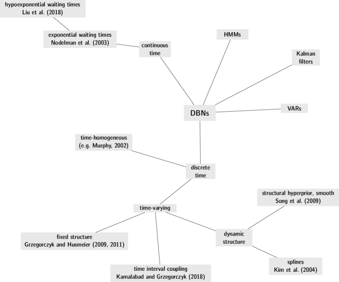
Figure 1: Diagram illustrating the relationships between the papers and the approaches covered in Section 3.

These choices are motivated by computational and statistical simplicity: there is no intrinsic limitation in the construction of DBNs that prevents them from modelling dependencies that stretch further back in time or, for that matter, trends or seasonality. (See Figure 1 for an overview of the models we will discuss in detail below.) Grzegorczyk and Husmeier [47, 48], for instance, constructed non-stationary, non-homogeneous DBNs for modelling continuous data using change-points to capture different regimes in different time intervals; they balanced this increased flexibility by requiring $\mathcal{G}$ to be the same for all regimes, allowing only the parameters of the local distributions to change. This restriction was later relaxed in Kamalabad and Grzegorczyk [56] by allowing both $\mathcal{G}$ and the parameters to vary but coupling them between adjacent time intervals. The hyperparameters controlling the coupling were allowed to vary between segments, following an inverse Gamma hyperprior. Robinson and Hartemink [95] also defined a non-stationary DBN with change-points and associated arc changesets, with truncated geometric priors on the size of the changesets, number of and interval between change-points; and Song et al. [112] constructed DBNs that vary smoothly (not piecewise) over time in both structure and parameters. Kim et al. [57] introduced an even more flexible model that used spline regression with B-splines to identify $\Pi_{X_{i}^{(t)}}$. Augmenting temporal (panel) data with non-temporal (cross-sectional) data for learning DBNs has been explored as well by Lähdesmäki and Shmulevich [60] using an score that approximates the resulting intractable likelihood.

Modelling DBNs as discrete time processes is likewise a choice motivated by mathematical simplicity. Nodelman et al. [83] originally proposed a class of continuous-time DBNs (CTBNs) with independent exponential waiting times and discrete nodes; they are uniquely identifiable since all arcs are non-instantaneous, and they have a closed-form marginal likelihood as well. More recently, this work has been expanded in Liu et al. [68] by replacing exponential waiting times with hypoexponentials to better reflect the behaviour of data in several domains. Discrete-time DBNs are certainly simpler than any of these CTBNs, but that mathematical simplicity comes with important practical consequences. Firstly, in order to work in discrete time we must choose a uniform time step (the length of time between $t-1$ and $t$) for the whole DBN; but in many real-world phenomena different variables can have very different time granularities, and those time granularities may vary as well in the course of data collection, making any single choice for the time step inappropriate. Secondly, the choice of the time step may obscure the dynamics of the phenomenon. The implication of using discrete time is that we aggregate all the state changes in the DBN over the entire course of each time step. On the one hand, if variables evolve at slower pace than the time step we are forced to model the DBN as a higher-order Markov process, resulting in a much more complex model. On the other hand, if variables evolve at a faster pace than time step, this averaging will effectively hide state changes and their interplay into a single summary statistic; hence the DBN will provide a very poor approximation of the underlying phenomenon. Furthermore, if we are unable to correctly identify the $\Pi_{X_{i}^{(t)}}$, $X_{i}^{(t)}$ may end up being recursively linked to the parents of the $\Pi_{X_{i}^{(t)}}$, resulting into dense DBNs that are much more complex than the real underlying phenomenon and that are difficult to learn from limited data.

A partial solution to the latter problem is to allow the parents $\Pi_{X_{i}^{(t)}}$ to be either in the same time or in the previous time point, modelling the DBN as a first-order Markov process. When observations represent average or aggregate measurements over a period of time (say, the $t$th time point corresponds to the $t$th week’s worth of data), it makes sense to allow instantaneous dependencies between variables in the same time point, since the instantaneousness of the dependence is just a fiction arising from our model definition. On the other hand, when observations actually correspond to instantaneous measurements (such as from synchronised sensors) only non-instantaneous dependencies are usually allowed in the model, on the grounds that conditioning event ($\Pi_{X_{i}^{(t)}}=\pi_{X_{i}^{(t)}}$) should precede in time the conditioned event ($X_{i}^{(t)}=x_{i}^{(t)}$). From a causal perspective, we can similarly argue that each of the $\Pi_{X_{i}^{(t)}}$ can only cause $X_{i}^{(t)}$ if it precedes $X_{i}^{(t)}$ in time; if that $\Pi_{X_{i}^{(t)}}$ is in the same time point as $X_{i}^{(t)}$ then what we are modelling is co-occurrence and not causation. This the core idea of Granger causality [46], which states that one time series (such as the $\Pi_{X_{i}^{(t)}}$) can be said to have a causal influence on a second time series (such as the $X_{i}^{(t)}$) if and only if incorporating past knowledge about the former improves predictive accuracy for the latter. Therefore, allowing instantaneous dependencies makes causal reasoning on the DBN markedly more difficult. The same is true for learning the structure of the DBN in the first place: learning a general BN is NP-hard [19, 21], while learning a DBN containing only non-instantaneous dependencies is not [29]. Intuitively, the space of the possible DBNs is much smaller if we do not allow instantaneous dependencies because there are fewer candidate arcs that we can include, and because their directions are fixed to follow the arrow of time and Granger causality.

3.2 Models That Can Be Expressed as DBNs

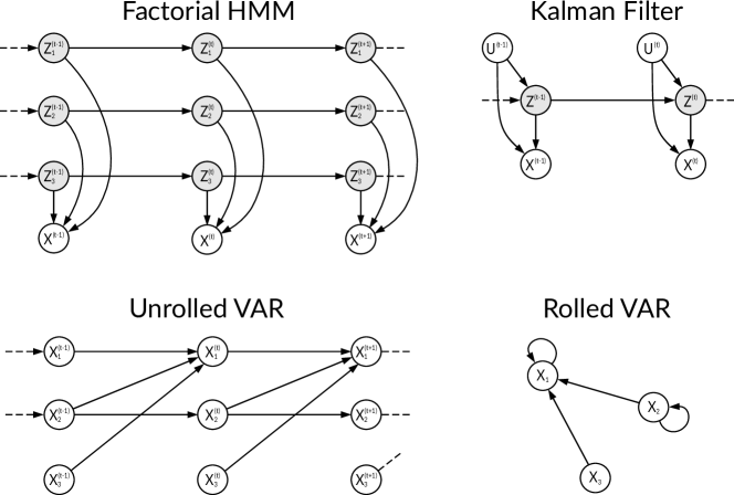
Figure 2: Dynamic models represented as BNs: the factorial HMM from Ghahramani and Jordan [45, top left], a simple Kalman filter model from Murphy [78, top right], and a VAR model of order 1 in both unrolled (bottom left) and rolled forms (bottom right). Shaded nodes correspond to latent variables.

DBNs have a strong expressive power, and they subsume and generalise a variety of classic models that have been studied individually in the literature. Here we will discuss three such models: hidden Markov models, vector auto-regressive models and Kalman filters. Hidden Markov models and Kalman filters can be seen as particular instances of state-space models, and their DBN representations make clear the relationship between these two classes of models. Representing these models as DBNs has advantages beyond making their comparison more convenient; it makes it possible to use the probabilistic machinery we covered in Sections 2 and 3.1 when more convenient or computationally efficient than the alternatives [as in the case of inference in hidden Markov models; 78]. Some examples are shown in Figure 2, and will be illustrated below.

Hidden Markov models [HMMs; 124] are one of the most widespread approaches to model phenomena with hidden state, that is, in which the behaviour of the observed variables $\mathbf{X}$ depends on that of one or more discrete latent variables $\mathbf{Z}$ as well as on other variables in $\mathbf{X}$. This scenario commonly arises when technical, economic or ethical considerations make it unfeasible to completely observe the underlying state of the phenomenon of interest. Notable examples are imputation [73] and phasing [28] in genome-wide association studies, due to limitations in the technology to probe and tag DNA; tracking animals in ecology [85], where we can observe their movements using radio beacons but not their behaviour; and confirming mass migrations through history by combining archaeological artefacts and ancient DNA samples [104]. Until the advent of deep neural networks, HMMs were also the choice model for speech [40] and handwriting recognition [90].

In DBN terms, a typical HMM model with $M$ latent variables can be written as

$$\operatorname{P}\left(\mathbf{X}^{(t)}\operatorname{|}\mathbf{X}^{(t-1)},\mathbf{Z}^{(t)}\right)=\prod_{i=1}^{N}\operatorname{P}\left(X_{i}^{(t)}\operatorname{|}\Pi_{X_{i}^{(t)}},\mathbf{Z}^{(t)}\right) \operatorname{P}\left(\mathbf{Z}^{(t)}\right)=\prod_{j=1}^{M}\operatorname{P}\left(Z_{j}^{(t)}\operatorname{|}\Pi_{Z_{j}^{(t)}}\right),$$ and (8)

with the restriction that the parents of $Z_{j}^{(t)}$ can only be other latent variables. Latent variables are assumed to be discrete; and in the vast majority of the literature observed variables are assumed to be discrete as well. Depending on the choice of $\Pi_{Z_{j}^{(t)}}$, we can obtain various HMM variants such as hierarchical HMMs [34], in which each $Z_{j}^{(t)}$ is defined as an HMM itself to produce a multi-level stochastic model; and factorial HMMs [45], in which the $\mathbf{X}^{(t)}$ are driven by the configuration of a set of mutually independent $Z_{j}^{(t)}$ (shown in Figure 2, top-left panel).

Vector auto-regressive models [VARs; 12] are a straightforward multivariate extension of univariate auto-regressive time series for continuous variables. As such, their major applications are forecasting in finance [7] and more recently in the analysis of fMRI data [41]. They are defined as

$$\mathbf{X}^{(t)}=A_{1}\mathbf{X}^{(t-1)}+\ldots+A_{L}\mathbf{X}^{(t-L)}+\varepsilon_{t}, \varepsilon_{t}\sim N(0,\Sigma),A_{1},\ldots A_{L}\in\mathbb{R}^{N\times N},$$ (9)

for some fixed Markov order $L$. We can rewrite (9) as

$$\mathbf{X}^{(t)}\operatorname{|}\mathbf{X}^{(t-1)},\ldots,\mathbf{X}^{(t-L)}\sim N\left(A_{1}\mathbf{X}^{(t-1)}+\ldots+A_{L}\mathbf{X}^{(t-L)},\varepsilon_{t}\right)$$

and then restrict the parents of each $X_{i}^{(t)}$ to those for which the corresponding regression coefficients in $A_{1},\ldots,A_{L}$ are different from zero using the one-to-one correspondence between regression coefficients and partial correlations [119]. Formally, $X_{j}^{(t-l)}\in\Pi_{X_{i}^{(t)}}$ if and only if $A_{l}[i,j]\neq 0$, which makes it possible to write (9) in a similar form to (6) and obtain a Gaussian DBN. The same construction is used by Song et al. [112] for their non-homogeneous DBN models, which are parameterised as VAR processed and estimated using $L_{1}$-penalised regressions. In the special case in which $L=1$, VARs can be graphically represented in two equivalent ways shown in the bottom panels of Figure 2: an “unrolled” DBN in which each node corresponds to a single $X_{i}^{(t)}$; and a more compact “rolled-up” DBN in which each node corresponds to a variable $X_{i}$, an arc from $X_{i}$ to $X_{j}$ implies $X_{i}^{(t-1)}\to X_{j}^{(t)}$. An arc from $X_{i}$ to itself implies $X_{i}^{(t-1)}\to X_{i}^{(t)}$ as a special case for $i=j$.

Kalman filters [KFs; 50] combine traits of both HMMs and VARs, as discussed in depth in Roweis and Ghahramani [97] and Ghahramani [44]: like VARs, they are linear Gaussian DBNs; but they also have latent variables like HMMs. They are widely used for filtering (that is, denoising) and prediction in GPS positioning systems [120]; atmospheric modelling and weather prediction [14]; and seismology [101]. In their simplest form (see Figure 2, top-right panel), KFs include a layer of one or more latent variables that model the unobservable part of the phenomenon,

$$\mathbf{Z}^{(t)}=A\mathbf{Z}^{(t-1)}+B\mathbf{U}^{(t)}+\zeta_{t}, \zeta_{t}\sim N(0,\Psi),A\in\mathbb{R}^{M\times M},B\in\mathbb{R}^{M\times P}$$

feeding into one or more observed variables

$$\mathbf{X}^{(t)}=C\mathbf{Z}^{(t)}+D\mathbf{U}^{(t)}+\varepsilon_{t}, \varepsilon_{t}\sim N(0,\Sigma),C\in\mathbb{R}^{N\times M},D\in\mathbb{R}^{N\times P}$$

with independent Gaussian noise added in both layers. Both layers often include additional (continuous) explanatory variables $\mathbf{U}$ and can also be augmented with (discrete) switching variables to allow for different regimes as in Grzegorczyk and Husmeier [47, 48]. If we exclude the latter, the assumption is that the system is jointly Gaussian: that makes it possible to frame KFs as a DBN in the same way we did for VARs.

4 Bayesian Networks from Incomplete Data

The vast majority of the literature on learning BNs rests on the assumption that $\mathcal{D}$ is complete, that is, a data set in which every variable has an observed value for each sample. However, in real-world applications we frequently have to deal with incomplete data; some samples will be completely observed while others will contain missing values for some of the variables. While it is tempting to simply impute the missing values as a preprocessing step, it has long been known that even fairly sophisticated techniques like hot-deck imputation are problematic in a multivariate setting [55]. Just deleting incomplete samples can also bias learning, depending on how missing data are missing.

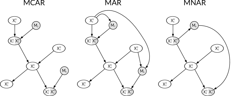
Figure 3: BN representations of the MCAR (left), MAR (centre) and MNAR (right) patterns of missingness from Rubin [98] and Little and Rubin [67]. Shaded nodes and portion of nodes correspond to variables that are not observed in the data.

Rubin [98] and Little and Rubin [67] formalised three possible patterns (or mechanisms) of missingness (illustrated in Figure 3):

• Missing completely at random (MCAR): when complete samples are indistinguishable from incomplete ones. In other words, the probability that a value will be missing is independent from both observed and missing values. For instance, in the left panel of Figure 3 both $X_{2}$ and $X_{6}$ are only partially observed; hence $X_{2}=(X_{2}^{O},X_{2}^{M})$ and $X_{6}=(X_{6}^{O},X_{6}^{M})$ where $X_{2}^{0}$ and $X_{6}^{O}$ are observed and $X_{2}^{M}$ and $X_{6}^{M}$ are missing. The patterns of missingness are controlled by $M_{2}$ (for $X_{2}$) and $M_{6}$ (for $X_{6}$) and are completely random; say, $M_{2}$ and $M_{6}$ are binary variables that encode the probability of two instruments (independently) breaking down and thus failing to measure $X_{2}$ and $X_{6}$ for some individuals.

• Missing at random (MAR): cases with incomplete data differ from cases with complete data, but the pattern of missingness is predictable from other observed variables. In other words, the probability that a value will be missing is a function of the observed values. An example is the central panel of Figure 3: compared to the left panel, we now know that the two instruments are likely to fail when (say) high values of $X_{1}$ (and $X_{3}$, in the case of $X_{6}$) are observed.

• Missing not at random (MNAR): the pattern of missingness is not random or it is not predictable from other observed variables; the probability that an entry will be missing depends on both observed and missing values. Common examples are variables that are missing systematically or for which the patterns of missingness depends on the missing values themselves. In the right panel of Figure 3, say that $X_{2}$ is censored (that is, it is never observed if its value is higher than a fixed threshold); but when $X_{2}$ is missing the probability that $X_{6}$ is missing (encoded by $M_{6}$) is also extremely high. Since we never observe $X_{2}$ when $X_{6}$ is missing, we are unable to correctly model this relationship; as far as we know both $X_{2}$ and $X_{6}$ may be missing due to some common external factor, since they appear to be missing together in the data.

MCAR and MAR are ignorable patterns of missingness; the probability that some value is missing may depend on observed values but not on missing values, and thus can be properly modelled. If we denote with $\mathcal{D}^{O}$ and $\mathcal{D}^{M}$ the observed and unobserved portions of $\mathcal{D}$, and we group all the binary missingness indicators $M_{i}$ in $\mathbf{M}$ with parameters $\Xi$, then we can write

$$\operatorname{P}\left(\mathcal{D},\mathbf{M}\operatorname{|}\mathcal{G},\Theta,\Xi\right)=\operatorname{P}\left(\mathcal{D}^{O},\mathcal{D}^{M},\mathbf{M}\operatorname{|}\mathcal{G},\Theta,\Xi\right)=\int\operatorname{P}(\mathcal{D}^{O},\mathcal{D}^{M}\operatorname{|}\mathcal{G},\Theta)\operatorname{P}\left(\mathbf{M}\operatorname{|}\mathcal{D}^{O},\mathcal{D}^{M},\mathcal{G},\Xi\right)\,d\mathcal{D}^{M};$$ (10)

if the missing data are MAR then $\mathbf{M}$ only depends on $\mathcal{D}^{O}$,

$$\operatorname{P}\left(\mathbf{M}\operatorname{|}\mathcal{D}^{O},\mathcal{D}^{M},\mathcal{G},\Xi\right)=\operatorname{P}\left(\mathbf{M}\operatorname{|}\mathcal{D}^{O},\mathcal{G},\Xi\right);$$

and if the missing data MCAR then $\mathbf{M}$ does not depend on either $\mathcal{D}^{O}$ or $\mathcal{D}^{M}$,

$$\operatorname{P}\left(\mathbf{M}\operatorname{|}\mathcal{D}^{O},\mathcal{D}^{M},\mathcal{G},\Xi\right)=\operatorname{P}\left(\mathbf{M}\operatorname{|}\mathcal{G},\Xi\right).$$

In both cases it is possible to model $\mathbf{M}$ from the available data. However, this is not the case for MNAR since $\mathbf{M}$ depends on the unobserved $\mathcal{D}^{M}$.

Modelling incomplete data is analytically intractable and computationally prohibitive compared to the complete data scenario: an exact analysis requires the computation of the joint posterior distribution of $\Theta$ considering all possible completions of $\mathcal{D}$. However, completing $\mathcal{D}$ has a computational complexity that grows exponentially with the number of missing entries, since it involves finding the set of missing data completions with the highest joint probability given the observed data. Considering just the most probable completion can also induce over-confidence in the results of the analysis, since completed observations will have lower variability by construction; but full Bayesian inference averaging over all possible $\Theta$ and completed $\mathcal{D}$ is so computationally challenging as to be unfeasible even in simple settings. Furthermore, this joint maximisation breaks the parameter independence assumption and makes it impossible to define decomposable scores for structure learning without resorting to some approximation.

4.1 Parameter Learning

Figure 4: Diagram illustrating the relationships between the papers and the approaches covered in Section 4.

Many approaches have been developed for parameter learning from incomplete data given a fixed, known structure, ranging from iterative methods like Data Augmentation [DA; 115] and the Expectation-Maximisation algorithm [EM; 62], to methods based on probability intervals such as Bound and Collapse [BC; 91] and uncertain probabilities [26]. (See Figure 4 for an overview of those we will discuss in detail below.) These methods usually assume missing data are MCAR or MAR to work on $\operatorname{P}(\Theta,\mathcal{D}^{M}\operatorname{|}\mathcal{G},\mathcal{D}^{O})$, and their accuracy decreases dramatically if that is not the case [113]; however, BC has been found to be robust also for MNAR data. Oniśko et al. [84] also noted that simple imputation approaches can perform well in learning the parameters of a BN given a fixed, sparse network structure, which further expands available options.

In the context of parameter learning, the EM algorithm retains its classic structure:

• the expectation (E) step consists in computing the expected values of the sufficient statistics (such as the counts $n_{ijk}$ in discrete BNs, partial correlations in GBNs), using exact inference along the lines described above to make use of incomplete as well as complete samples;

• the maximisation (M) step takes the sufficient statistics from the E-step and estimates the parameters of the BN, either using maximum likelihood or Bayesian posterior estimators.

The parameter estimates are then used in the next E-step to update the expected values of the sufficient statistics; repeated iterations of these two steps will in the limit return the maximum likelihood or maximum a posteriori estimates for the parameters. Using the notation of (10), the E-step is equivalent to computing $\operatorname{E}(\mathcal{D}^{M},\mathcal{D}^{O}\operatorname{|}\mathcal{G},\Theta)$ and the M-step to maximising $\operatorname{P}(\Theta\operatorname{|}\mathcal{G},\mathcal{D}^{O},\mathcal{D}^{M})$.

DA is quite similar, but instead of converging iteratively to a single set of parameter estimates it uses Gibbs Sampling [43] to generate values from the posterior distributions of both $\mathcal{D}^{M}$ and $\Theta$. The two steps are as follows:

• in the imputation (I) step the data are completed with values drawn from the predictive distributions of the missing values;

• in the parameter (P) estimation step a parameter value is drawn from the posterior distribution of $\Theta$ conditional on the completed data from the I-step.

More formally, we define the augmented parameter vector $\{\mathcal{D}^{M},\Theta\}$ containing both the missing values and the parameters of the BN. Given an initial set of values, it updates each element of $\{\mathcal{D}^{M},\Theta\}$ by sampling a new value for each missing value from $\operatorname{P}(\mathcal{D}^{M}_{i}\operatorname{|}\mathcal{D}^{M}_{-i},\Theta)$, and by sampling a new value for each parameter from $\operatorname{P}(\Theta_{i}\operatorname{|}\Theta_{-i},\mathcal{D}^{M})$, each in turn. After an initial burn-in phase, this process will converge to its stationary distribution and return parameter realisations from the posterior distribution of $\Theta$ conditional on the observed data. A similar Gibbs sampling approach has been proposed more recently by Riggelsen [94]: it samples from a simpler, approximate predictive distribution and makes use of weights to implement an efficient importance sampling scheme. In addition, the weights make it possible to use samples generated in the burn-in phase as well as those from the stationary distribution of the Gibbs samples because they weight samples according to their estimated predictive accuracy.

Finally, BC and its successor the Robust Bayesian Estimator [RBE; 92] exploit the discrete nature of categorical variables to produce rough interval estimates of the conditional probabilities learned from incomplete variables, which are then reduced to point estimates either via a convex combination of the intervals’ bounds, expert knowledge or both. The first (bound) step, uses the fact that each $\pi_{ik\operatorname{|}j}$ can be bounded below by assuming that none of the missing values for $X_{i}$ are completed with their $k$th value when the $j$th parent configuration is observed; and that $\pi_{ik\operatorname{|}j}$ can be bounded above by assuming that all missing values are completed with their $k$th value. This approach has the merit of not making any assumptions on the distribution of missing data. Furthermore, the width of each interval provides an explicit representation of the reliability of the estimates, which can be taken into account in inference and prediction. The second (collapse) step assumes missing data are MAR or MCAR to be able to compute the expected completions for incomplete samples, which are then used to compute the mean and variance of the $\pi_{ik\operatorname{|}j}$. Interestingly, the intervals from the bound step can be used to augment both EM and Gibbs sampling and obtain more precise inferences, but the predictive accuracy of RBE was shown to be superior to both in Ramoni and Sebastiani [92]. A similar investigation in the context of BN classifiers can be found in Peña et al. [88]. A conceptually similar approach was also proposed by Liao and Ji [65], which first used qualitative expert knowledge on the parameter values to bound them, and then estimated their values using convex optimisation embedded in the EM algorithm.

Note that we can work on latent variables using similar approaches as long as $\mathcal{G}$ is fixed and we just need to learn $\Theta$. A recent example is given in Yamazaki and Motomura [121], who show it is possible to learn the domain of a latent discrete variable as well as the associated parameters as long as it has observed parents and children. Several other examples are discussed in the context of DBNs in Murphy [78].

4.2 Structure Learning

Learning the structure of a BN from incomplete data is, in many respects, an extension of the techniques covered in Section 4.1. (See Figure 4 for an overview of the approaches we will discuss in detail below as well as those for parameter learning.) In its general form it is computationally unfeasible because we need to perform a joint optimisation over the missing values and the parameters to score each candidate network. Starting from (4), we can make this apparent by rewriting $\operatorname{P}(\mathcal{D}\operatorname{|}\mathcal{G})$ as a function of $\mathcal{D}^{O},\mathcal{D}^{M}$:

$$\operatorname{P}\left(\mathcal{D}\operatorname{|}\mathcal{G}\right)=\operatorname{P}\left(\mathcal{D}^{O},\mathcal{D}^{M}\operatorname{|}\mathcal{G}\right)=\int\operatorname{P}\left(\mathcal{D}^{O},\mathcal{D}^{M}\operatorname{|}\mathcal{G},\Theta\right)\operatorname{P}\left(\Theta\operatorname{|}\mathcal{G}\right)\,d\Theta=\\ =\int\underbrace{\operatorname{P}\left(\mathcal{D}^{M}\operatorname{|}\mathcal{D}^{O},\mathcal{G},\Theta\right)}_{\text{missing data}}\underbrace{\operatorname{P}\left(\mathcal{D}^{O}\operatorname{|}\mathcal{G},\Theta\right)}_{\text{observed data}}\underbrace{\operatorname{P}\left(\Theta\operatorname{|}\mathcal{G}\right)\,d\Theta}_{\text{averaging over parameters}}.$$ (11)

From this expression we can see that in order to maximise $\operatorname{P}(\mathcal{D}\operatorname{|}\mathcal{G})$ we should jointly maximise the probability of the observed data $\mathcal{D}^{O}$ and the probability of the missing data $\mathcal{D}^{M}$ given the observed data, for each candidate $G$ and averaging over all possible $\Theta$. This gives us the maximum a posteriori solution to structure learning; a full Bayesian approach would require averaging over all the possible configurations of the missing data as well, leading to

$$\operatorname{P}\left(\mathcal{D}\operatorname{|}\mathcal{G}\right)=\iint\operatorname{P}\left(\mathcal{D}^{M}\operatorname{|}\mathcal{D}^{O},\mathcal{G},\Theta\right)\operatorname{P}\left(\mathcal{D}^{O}\operatorname{|}\mathcal{G},\Theta\right)\operatorname{P}\left(\Theta\operatorname{|}\mathcal{G}\right)\,d\Theta\,d\mathcal{D}^{M}.$$ (12)

Compared to (11), (12) contains one extra dimension for each missing value (in addition to one dimension for each parameter in $\Theta$) and thus it is too high-dimensional to compute in practical applications. An additional problem is that, while $\operatorname{P}(\mathcal{D}^{O}\operatorname{|}\mathcal{G},\Theta)$ decomposes as in (5), $\operatorname{P}(\mathcal{D}^{M}\operatorname{|}\mathcal{D}^{O},\mathcal{G},\Theta)$ does not in the general case.

In order to sidestep these computational issues, the literature has pursued two possible approaches: iteratively completing and refining the data, an using standard algorithms and scores for complete data; or using scoring functions that approximate BIC and $\operatorname{P}(\mathcal{D}\operatorname{|}\mathcal{G})$ but that are decomposable and can be computed efficiently even on incomplete data.

The Structural EM algorithm [SEM; 36] is the most famous implementation of the first approach; it has important applications in phylogenetics [38], clinical record [118] and clinical trial analysis [66]. SEM makes structure learning computationally feasible by searching for the best structure inside of EM, instead of embedding EM inside a structure learning algorithm. It consists of two steps like the classic EM:

• in the E-step, we complete the data by computing the expected sufficient statistics using the current network structure;

• in the M-step, we find the structure that maximises the expected score function for the completed data.

Since the scoring in the M-step uses the completed data , structure learning can be implemented efficiently using standard algorithms. The original proposal by Friedman [36] used BIC and greedy search; Friedman [37] later extended SEM to a fully Bayesian approach based posterior scores, and proved the convergence of the resulting algorithm.

In fact, any combination of structure learning algorithm and score can be used in the M-step; most recently Scanagatta et al. [103] proposed learning BNs with a bounded-treewidth structure using their k-MAX algorithm and a variant of BIC. (This has the two-fold advantage of speeding up the M-step and of yielding BNs for which completing data in the E-step is relatively fast.) Singh [111] proposed a similar approach based on DA, generating sets of completed data sets and averaging the resulting learned networks in each iteration. Myers et al. [80] also chose to iteratively learn both the network structures and the missing data at the same time, but did so using evolutionary algorithms and encoding both as “genes”. Hence, the individuals in the population being evolved comprise both a completed data set and the associated BN. This was combined with Metropolis-Hastings to speed up learning as discussed in Myers et al. [79].

More recently, Adeel and de Campos [1] proposed an exact learning algorithm that explicitly models the patterns of missingness with auxiliary variables, which are included as separate nodes in the BN rather than just being computational devices. Additionally, they showed that its computational complexity is the same as that of other exact learning algorithms for complete data; and they adapted the proposed algorithm into a (faster) heuristic that is then proven to be consistent.

The second group of approaches includes the variational-Bayesian EM from Beal and Ghahramani [10] that maximises a variational approximation of $\operatorname{P}(\mathcal{D}\operatorname{|}\mathcal{G})$, which in turn is a lower bound to the true marginal likelihood. Balov [5] proved that structure learning with BIC is not consistent even under MCAR, and suggested replacing it with node-average penalised log-likelihoods computed from locally complete observations. An alternative consists in using approximations based on mixtures of truncated exponentials, as was showcased in Fernández et al. [33]: they combined EM and DA to fit regression-like BNs with structures that resemble naive Bayes and tree-augmented naive Bayes classifiers, and approximating explanatory variables. Approachable introductions to this area of research are provided in Chickering and Heckerman [20] and Heckerman [51], which describe the relationship between $\operatorname{P}(\mathcal{D}\operatorname{|}\mathcal{G})$, its Laplace approximation and BIC in mathematical detail.

5 Software and Applications

To conclude this review, we consider the practicalities of using the BN models discussed above to investigate real-world problems: the availability of software implementations and notable examples of applications in various fields.

5.1 Available Software

Among the DBN papers we covered, only Grzegorczyk and Husmeier [47, 48] and [60] provide implementations of the methods they propose as Matlab scripts available upon request from the authors. Additionally, Liu et al. [68] provides links to the custom software they use in the paper. Hugin [4] implements discrete-time, homogeneous DBNs as defined in (6), as does GeNIe [9].

Software implementations for handling incomplete are more readily available, even though typically not from the papers that propose the methods. Both Hugin and GeNIe implement EM for parameter learning, but not Structural EM for parameter learning. The R packages bnlearn [106] and bnstruct [35] implement the structural EM algorithm; another implementation in Matlab is made available as part of the supplementary material of [93]. Adeel and de Campos [1] have later used it to implement their exact learning algorithm along with Gobnilp [8]; and [94] uses a custom C++ implementation of his Gibbs sampling approach. The approaches proposed by Balov [5] are implemented in the catnet R package [6], and those proposed by Fernández et al. [33] are included in Elvira [31].

5.2 Notable Applications

Dynamic and incomplete data are common in many application fields in which BNs are used; the need to work with such data is the main motivation for developing the approaches we covered in Sections 3 and 4. Therefore, many of them have been used in advanced applications especially in the clinical and life sciences.

This is especially true for DBNs: since they subsume a number of statistical models that are themselves very popular (see Section 3.2), it would be fair to say that they are used in most branches of science under different guises. However, their main application fields in the literature remain genetics and systems biology, and in particular the modelling of cell signalling pathways in the form of networks as they evolve over time. This involves probing the state of multiple proteins or other omics simultaneously through time, and studying their interactions and how they evolve in response to external stimuli. In vitro experiments, in which cell lines are probed in a controlled environment, have been modelled as homogeneous DBNs [see, for instance, 53, 89]. On the other hand, more complex and in vivo experiments often involve molecular systems that are not in a steady-state regime and thus require non-homogeneous DBNs. Some examples based on the models presented in Grzegorczyk and Husmeier [47, 48], Kamalabad and Grzegorczyk [56] and other papers from the same authors study embryonic stem cells [74]; sepsis as a cause of acute lung injury [32]; blunt trauma and traumatic spinal cord injury association with inflammation [122] and hypotension [3]. Other omics data including transcriptomics [69] and microbiome data [75, 70] have been studied using DBNs as well.

DBNs have also seen application in ecology, specifically in studying species dynamics. Like the human body, an ecosystem acts as a complex system where species interact with each other (for example, through predation or competition) and with the environment they live in. The resulting dynamics have been modelled in Aderhold et al. [2] with the non-homogeneous DBN from Grzegorczyk and Husmeier [48]. A DBN that corrects for spatial correlation as well through the use of latent variables have been developed in Trifonova et al. [117] to study fish species dynamics in 7 geographically and temporally varied areas within the North Sea. Furthermore, ecosystems have been studied using DBNs from the point of view of environmental sciences as well, considering for example the impact of climate change on groundwater [76] and how to best manage water reservoirs under infrequent rainfalls [96].

Finally, a third class of applications of DBNs is modelling mechanical systems in engineering, reliability and quality control studies. For instance, studying the deterioration of steel structures subject to fatigue [71] including warships [64]; implementing real-time reliability monitoring of subsea pipes [13] and CNC industrial systems [116]; fault detection, identification and recovery in autonomous spacecrafts [22]; and predicting traffic dynamics using probes in San Francisco [54] In each of these applications, DBNs capture the interactions of the components of the mechanical systems they are modelling while at the same time incorporating the effects of the surrounding environment, thus allowing the operators (or the systems itself) to adjust its mode of operation or to stop it completely before causing any damage or safety issue. Software systems have been similarly modelled, for example to study the relationship between security vulnerabilities and attack vectors in network security [39].

As for incomplete data, they are such a widespread issue in science and engineering that it is difficult to identify any particular field in which they are prevalent; hence the BN learning approaches in Section 4 have found very different applications in the literature. We note, however, that the analysis of clinical data has historically been one of the key applications that has driven methodological developments in this area. We mentioned earlier the study of clinical records of patients chronic obstructive pulmonary disease [118] and the recovery process of patients with whiplash-associated disorders [66]; two other examples are the diagnosis of brain diseases such as dementia and Alzheimer [110] and of sleep apnea [100]. Completely different applications have also been explored: one example is the classification of radar images [72].

6 Summary

In this paper we have reviewed the fundamental definitions and properties of BNs, and how BNs can be stretched to encode more complex probabilistic models than what might be apparent from reference material and most of the literature. Both have an overwhelming focus on the straightforward case in which the data being modelled are both static (that is, with no time dimension) and complete (that is, with no missing values). However, dynamic and incomplete data are central to many cutting-edge applications in research fields ranging from genetics to robotics; BNs can play an important role in many of these settings, as has been evidenced by the examples referenced in Sections 3 and 4. Given their expressive power, BNs also subsume several classic probabilistic models and can augment them with automatic reasoning capabilities through various kinds of queries that can be performed algorithmically. Much research has been and is being developed to adapt BNs to these applications and make them a competitive choice for modelling complex data.

References

- Adeel and de Campos [2017] T. Adeel and C. P. de Campos. Learning Bayesian Networks with Incomplete Data by Augmentation. In Proceedings of the 31st AAAI Conference on Artificial Intelligence, pages 1684–1690, 2017.
- Aderhold et al. [2012] A. Aderhold, D. Husmeier, J. J. Lennon, C. M. Beale, and V. A. Smith. Hierarchical Bayesian Models in Ecology: Reconstructing Species Interaction Networks from Non-Homogeneous Species Abundance Data. Ecological Informatics, 11:55–64, 2012.
- Almahmoud et al. [2015] K. Almahmoud, R. A. Namas, A. M. Zaaqoq, O. Abdul-Malak, R. Namas, R. Zamora, J. Sperry, T. R. Billiar, and Y. Vodovotz. Prehospital Hypotension Is Associated With Altered Inflammation Dynamics and Worse Outcomes Following Blunt Trauma in Humans. Critical Care Medicine, 43(7):1395–1404, 2015.
- Andersen et al. [1989] S. K. Andersen, K. G. Olesen, F. V. Jensen, and F. Jensen. Hugin – A Shell for Building Bayesian Belief Universes for Expert Systems. In Proceedings of the 11th International Joint Conference on Artificial Intelligence, pages 1080–1085, 1989.
- Balov [2013] N. Balov. Consistent Model Selection of Discrete Bayesian Networks from Incomplete Data. Electronic Journal of Statistics, 7(1):1047–1077, 2013.
- Balov and Salzman [2019] N. Balov and P. Salzman. catnet: Categorical Bayesian Network Inference, 2019. URL https://cran.r-project.org/web/packages/catnet.
- Bańbura et al. [2010] M. Bańbura, D. Giannone, and L. Reichlin. Large Bayesian Vector Auto Regressions. Journal of Applied Economics, 25(1):71–92, 2010.
- Bartlett and Cussens [2013] M. Bartlett and J. Cussens. Advances in Bayesian Network Learning Using Integer Programming. In Proceedings of the 29th Conference on Uncertainty in Artificial Intelligence, pages 182–191, 2013.
- BayesFusion [2019] BayesFusion. GeNie Modeler. 2019. URL https://www.bayesfusion.com/genie.
- Beal and Ghahramani [2003] M. J. Beal and Z. Ghahramani. The Variational Bayesian EM Algorithm for Incomplete Data: with Application to Scoring Graphical Model Structures. In Proceedings of the 7th Valencia International Meeting, pages 453–464, 2003.
- Bøttcher [2001] S. G. Bøttcher. Learning Bayesian Networks with Mixed Variables. In Proceedings of the 8th International Workshop in Artificial Intelligence and Statistics, 2001.
- Box et al. [2016] G. E. P. Box, G. M. Jenkins, G. C. Reinsel, and G. M. Ljung. Time Series Analysis: Forecasting and Control. Wiley, 5th edition, 2016.
- Cai et al. [2015] B. Cai, Y. Liu, Y. Ma, Z. Liu, Y. Zhou, and J. Sun. Real-Time Reliability Evaluation Methodology Based on Dynamic Bayesian Networks: A Case study of a Subsea Pipe Ram BOP system. ISA Transactions, 58:595–604, 2015.
- Cassola and Burlando [2012] F. Cassola and M. Burlando. Wind Speed and Wind Energy Forecast Through Kalman Filtering of Numerical Weather Prediction Model Output. Applied Energy, 99:154–166, 2012.
- Castelo and Siebes [2000] R. Castelo and A. Siebes. Priors on Network Structures. Biasing the Search for Bayesian Networks. International Journal of Approximate Reasoning, 24(1):39–57, 2000.
- Castillo et al. [1997] E. Castillo, J. M. Gutiérrez, and A. S. Hadi. Expert Systems and Probabilistic Network Models. Springer, 1997.
- Chickering [1996] D. M. Chickering. Learning Bayesian Networks is NP-Complete. In D. Fisher and H. Lenz, editors, Learning from Data: Artificial Intelligence and Statistics V, pages 121–130. Springer-Verlag, 1996.
- Chickering [2002] D. M. Chickering. Optimal Structure Identification With Greedy Search. Journal of Machine Learning Research, 3:507–554, 2002.
- Chickering and Heckerman [1994] D. M. Chickering and D. Heckerman. Learning Bayesian Networks is NP-hard. Technical Report MSR-TR-94-17, Microsoft Corporation, 1994.
- Chickering and Heckerman [1997] D. M. Chickering and D. Heckerman. Efficient Approximations for the Marginal Likelihood of Bayesian Networks with Hidden Variables. Machine Learning, 29(2/3):181–212, 1997.
- Chickering et al. [2004] D. M. Chickering, D. Heckerman, and C. Meek. Large-sample Learning of Bayesian Networks is NP-hard. Journal of Machine Learning Research, 5:1287–1330, 2004.
- Codetta-Raiteri and Portinale [2014] D. Codetta-Raiteri and L. Portinale. Dynamic Bayesian Networks for Fault Detection, Identification, and Recovery in Autonomous Spacecraft. IEEE Transactions on Systems, Man, and Cybernetics: Systems, 45(1):13–24, 2014.
- Cowell [2001] R. G. Cowell. Conditions Under Which Conditional Independence and Scoring Methods Lead to Identical Selection of Bayesian Network Models. In Proceedings of the 17th Conference on Uncertainty in Artificial Intelligence, pages 91–97, 2001.
- Cowell et al. [2007] R. G. Cowell, A. P. Dawid, S. L. Lauritzen, and D. J. Spiegelhalter. Probabilistic Networks and Expert Systems. Springer-Verlag, 2007.
- Cussens [2012] J. Cussens. Bayesian Network Learning with Cutting Planes. In Proceedings of the 27th Conference on Uncertainty in Artificial Intelligence, pages 153–160, 2012.
- de Campos et al. [1994] L. M. de Campos, J. F. Huete, and S. Moral. Probability Intervals: A Tool for Uncertain Reasoning. International Journal Uncertainty, Fuzziness and Knowledge-Based Systems, 2:167–196, 1994.
- de Campos et al. [2002] L. M. de Campos, J. M. Fernández-Luna, J. A. Gámez, and J. M. Puerta. Ant Colony Optimization for Learning Bayesian Networks. International Journal of Approximate Reasoning, 31(3):291–311, 2002.
- Delaneau et al. [2012] O. Delaneau, J. Marchini, and J.-F. Zagury. A Linear Complexity Phasing Method for Thousands of Genomes. Nature Methods, 9(2):179–181, 2012.
- Dojer [2006] N. Dojer. Learning Bayesian Networks Does Not Have to Be NP-Hard. In Mathematical Foundations of Computer Science, volume 4162 of Lecture Notes in Computer Science, pages 305–314. Springer, 2006.
- Druzdzel and van der Gaag [1995] M. J. Druzdzel and L. C. van der Gaag. Elicitation of Probabilities for Belief Networks: Combining Qualitative and Quantitative Information. In Proceedings of the 11th Conference on Uncertainty in Artificial Intelligence, pages 141–148, 1995.
- Elvira Consortium [2002] Elvira Consortium. An Environment for Creating and Using Probabilistic Graphical Models. In Proceedings of the 1st European Workshop on Probabilistic Graphical Models, pages 222–230. 2002.
- Emr et al. [2014] B. Emr, D. Sadowsky, N. Azhar, L. A. Gatto, G. An, G. Nieman, and Y. Vodovotz. Removal of Inflammatory Ascites is Associated with Dynamic Modification of Local and Systemic Inflammation along with Prevention of Acute Lung Injury: In Vivo and In Silico Studies. Shock, 41(4):317–323, 2014.
- Fernández et al. [2010] A. Fernández, J. D. Nielsen, and A. Salmerón. Learning Bayesian Networks for Regression from Incomplete Databases. International Journal of Uncertainty, Fuzziness and Knowledge-Based Systems, 18(01):69–86, 2010.
- Fine et al. [1998] S. Fine, Y. Singer, and N. Tibshy. The Hierarchical Hidden Markov Model: Analysis and Applications. Machine Laarning, 32(1):41–62, 1998.
- Franzin et al. [2017] A. Franzin, F. Sambo, and B. di Camillo. bnstruct: an R package for Bayesian Network Structure Learning in the Presence of Missing Data. Bioinformatics, 33(8):1250–1252, 2017.
- Friedman [1997] N. Friedman. Learning Belief Networks in the Presence of Missing Values and Hidden Variables. In Proceedings of the 14th International Conference on Machine Learning, pages 125–133, 1997.
- Friedman [1998] N. Friedman. The Bayesian Structural EM Algorithm. In Proceedings of the Fourteenth Conference on Uncertainty in Artificial Intelligence, pages 129–138, 1998.
- Friedman et al. [2002] N. Friedman, M. Ninio, I. Pe’er, and T. Pupko. A structural em algorithm for phylogenetic inference. Journal of Computational Biology, 9(2):331–353, 2002.
- Frigault et al. [2008] M. Frigault, L. Wang, A. Singhal, and S. Jajodia. Measuring Network Security Using Dynamic Bayesian Network. In Proceedings of the 14th ACM Workshop on Quality of Protection, pages 23–29, 2008.
- Gales and Young [2008] M. Gales and S. Young. The Application of Hidden Markov Models in Speech Recognition. Foundations and Trends in Signal Processing, 1(3):195–304, 2008.
- Gates et al. [2009] K. M. Gates, P. C. M. Molenaar, F. G. Hillary, N. Ram, and M. J. Rovine. Automatic Search for fMRI Connectivity Mapping: An Alternative to Granger Causality Testing Using Formal Equivalences Among SEM Path Modeling, VAR, and Unified SEM. NeuroImage, 50:1118–1125, 2009.
- Geiger and Heckerman [1994] D. Geiger and D. Heckerman. Learning Gaussian Networks. In Proceedings of the 10th Conference on Uncertainty in Artificial Intelligence, pages 235–243, 1994.
- Geman and Geman [1984] S. Geman and D. Geman. Stochastic Relaxation, Gibbs Distributions and the Bayesian Restoration of Images. IEEE Transactions on Pattern Analysis and Machine Intelligence, 6:721–741, 1984.
- Ghahramani [2001] Z. Ghahramani. An Introduction to Hidden Markov Models and Bayesian Networks. International Journal of Pattern Recognition and Artificial Intelligence, 15(1):9–42, 2001.
- Ghahramani and Jordan [1996] Z. Ghahramani and M. Jordan. Factorial Hidden Markov Models. In Advances in Neural Information Processing Systems, pages 472–278, 1996.
- Granger [1968] C. W. J. Granger. Investigating Causal Relations by Econometric Models and Cross-Spectral Methods. Econometrica, 37:424–438, 1968.
- Grzegorczyk and Husmeier [2009] M. Grzegorczyk and D. Husmeier. Non-Stationary Continuous Dynamic Bayesian Networks. In Advances in Neural Information Processing Systems, pages 682–690, 2009.
- Grzegorczyk and Husmeier [2011] M. Grzegorczyk and D. Husmeier. Non-homogeneous Dynamic Bayesian Networks for Continuous Data. Machine Learning, 83(3):355–419, 2011.
- Gupta and Kim [2008] S. Gupta and H. W. Kim. Linking Structural Equation Modeling to Bayesian Networks: Decision Support for Customer Retention in Virtual Communities. European Journal of Operational Research, 190(3):818–833, 2008.
- Hamilton [1994] J. D. Hamilton. Time Series Analysis. Princeton University Press, 1994.
- Heckerman [1997] D. Heckerman. Bayesian Networks for Data Mining. Data Mining and Knowledge Discovery, 1(1):79–119, 1997.
- Heckerman et al. [1995] D. Heckerman, D. Geiger, and D. M. Chickering. Learning Bayesian Networks: The Combination of Knowledge and Statistical Data. Machine Learning, 20(3):197–243, 1995. Available as Technical Report MSR-TR-94-09.
- Hill et al. [2012] S. M. Hill, Y. Lu, J. Molina, L. M. Heiser, P. T. Spellman, T. P. Speed, J. W. Gray, and G. B. Mills S. Mukherjee. Bayesian Inference of Signaling Network Topology in a Cancer Cell Line. Bioinformatics, 28(21):2804–2810, 2012.
- Hofleitner et al. [2012] A. Hofleitner, R. Herring, P. Abbeel, and A. Bayen. Learning the Dynamics of Arterial Traffic from Probe Data Using a Dynamic Bayesian Network. IEEE Transactions on Intelligent Transportation Systems, 13(4):1679–93, 2012.
- Kalton and Kasprzyk [1986] G. Kalton and D. Kasprzyk. The Treatment of Missing Survey Data. Surv. Methodol, 12:1–16, 1986.
- Kamalabad and Grzegorczyk [2018] M. S. Kamalabad and M. Grzegorczyk. Improving Nonhomogeneous Dynamic Bayesian Networks with Sequentially Coupled Parameters. Statistica Neerlandica, 72(3):281–305, 2018.
- Kim et al. [2004] S. Kim, S. Imoto, and S. Miyano. Dynamic Bayesian Network and Nonparametric Regression for Nonlinear Modeling of Gene Networks from Time Series Gene Expression Data. BioSystems, 75:57–65, 2004.
- Koller and Friedman [2009] D. Koller and N. Friedman. Probabilistic Graphical Models: Principles and Techniques. MIT Press, 2009.
- Korb and Nicholson [2010] K. Korb and A. Nicholson. Bayesian Artificial Intelligence. Chapman & Hall, 2nd edition, 2010.
- Lähdesmäki and Shmulevich [2008] H. Lähdesmäki and I. Shmulevich. Learning the Structure of Dynamic Bayesian Networks from Time Series and Steady State Measurements. Machine Learning, 71(2–3):185–217, 2008.
- Larrañaga et al. [1996] P. Larrañaga, M. Poza, Y. Yurramendi, R. H. Murga, and C. M. H. Kuijpers. Structure Learning of Bayesian Networks by Genetic Algorithms: a Performance Analysis of Control Parameters. IEEE Transactions on Pattern Analysis and Machine Intelligence, 18(9):912–926, 1996.
- Lauritzen [1995] S. L. Lauritzen. The EM Algorithm for Graphical Association Models with Missing Data. Computational Statistics and Data Analysis, 19(2):191–201, 1995.
- Lauritzen and Wermuth [1989] S. L. Lauritzen and N. Wermuth. Graphical Models for Associations Between Variables, Some of which are Qualitative and Some Quantitative. The Annals of Statistics, 17(1):31–57, 1989.
- Liang et al. [2017] X. F. Liang, H. D. Wang, H. Yi, and D. Li. Warship Reliability Evaluation Based on Dynamic Bayesian Networks and Numerical Simulation. Ocean Engineering, 136:129–140, 2017.
- Liao and Ji [2009] W. Liao and Q. Ji. Learning Bayesian Network Parameters under Incomplete Data with Domain Knowledge. Pattern Recognition, 42(11):3046–3056, 2009.
- Liew et al. [2019] B. X. W. Liew, M. Scutari, A. Peolsson, G. Peterson, M. L. Ludvigsson, and D. Falla. Investigating the Causal Mechanisms of Symptom Recovery in Chronic Whiplash Associated Disorders using Bayesian Networks. The Clinical Journal of Pain, 2019. In print.
- Little and Rubin [1987] R. J. A. Little and D. B. Rubin. Statistical Analysis with Missing Data. Wiley, 1987.
- Liu et al. [2018] M. Liu, F. Stella, A. Hommersom, and P. J. F. Lucas. Making Continuous Time Bayesian Networks More Flexible. Proceedings of Machine Learning Research (PGM 2018), 72:237–248, 2018.
- López-Kleine et al. [2013] L. López-Kleine, L. Leal, and C. López. Biostatistical Approaches for the Reconstruction of Gene Co-Expression Networks Based on Transcriptomic Data. Briefings in Functional Genomics, 12(5):457–467, 2013.
- Lugo-Martinez et al. [2019] J. Lugo-Martinez, D. Ruiz-Perez, G. Narasimhan, and Z. Bar-Joseph. Dynamic Interaction Network Inference from Longitudinal Microbiome Data. Microbiome, 7:54, 2019.
- Luque and Straub [2016] J. Luque and D. Straub. Reliability Analysis and Updating of Deteriorating Systems with Dynamic Bayesian Networks. Structural Safety, 62:34–46, 2016.
- Ma et al. [2016] F. Ma, Y.-W. Chen, X.-P. Yan, X.-M. Chu, and J. Wang. A Novel Marine Radar Targets Extraction Approach Based on Sequential Images and Bayesian Network. Ocean Engineering, 120:64–77, 2016.
- Marchini and Howie [2010] J. Marchini and B. Howie. Genotype Imputation for Genome-Wide Association Studies. Nature Reviews Genetics, 11(7):499–511, 2010.
- Mathew et al. [2015] S. Mathew, S. Sundararaj, and I. Banerjee. Network Analysis Identifies Crosstalk Interactions Governing TGF- Signaling Dynamics during Endoderm Differentiation of Human Embryonic Stem Cells. Processes, 3(2):286–308, 2015.
- McGeachie et al. [2016] M. J. McGeachie, J. E. Sordillo, T. Gibson, G. M. Weinstock, Y.-Y. Liu, D. R. Gold, S. T. Weiss, and A. Litonjua. Longitudinal Prediction of the Infant Gut Microbiome with Dynamic Bayesian Networks. Scientific Reports, 6:20359, 2016.
- Molina et al. [2013] J.-L. Molina, D. Pulido-Velázquez, J. L. García-Aróstegui, and M. Pulido-Velázquez. Dynamic Bayesian Networks as a Decision Support Tool for Assessing Climate Change Impacts on Highly Stressed Groundwater Systems. Journal of Hydrology, 479:113–129, 2013.
- Mukherjee and Speed [2008] S. Mukherjee and T. P. Speed. Network Inference Using Informative Priors. Proceedings of the National Academy of Sciences, 105(38):14313–14318, 2008.
- Murphy [2002] K. Murphy. Dynamic Bayesian Networks: Representation, Inference and Learning. PhD thesis, UC Berkeley, Computer Science Division, 2002.
- Myers et al. [1999a] J. W. Myers, K. B. Laskey, and K. A. DeJong. Learning Bayesian Networks from Incomplete Data Using Evolutionary Algorithms. In Proceedings of the 1st Annual Conference on Genetic and Evolutionary Computation, pages 458–465, 1999a.
- Myers et al. [1999b] J. W. Myers, K. B. Laskey, and T. S. Levitt. Learning Bayesian Networks from Incomplete Data with Stochastic Search Algorithms. In Proceedings of the 15th Conference on Uncertainty in Artificial Intelligence, pages 467–485, 1999b.
- Neapolitan [1989] R. E. Neapolitan. Probabilistic Reasoning in Expert Systems: Theory and Algorithms. 1989.
- Neapolitan [2003] R. E. Neapolitan. Learning Bayesian Networks. Prentice Hall, 2003.
- Nodelman et al. [2003] U. Nodelman, C. R. Shelton, and D. Koller. Learning Continuous Time Bayesian Networks. In Proceedings of the 19th Conference on Uncertainty in Artificial Intelligence, pages 451–458, 2003.
- Oniśko et al. [2002] A. Oniśko, M. J. Druzdzel, and H. Wasyluk. An Experimental Comparison of Methods for Handling Incomplete Data in Learning Parameters of Bayesian Networks. In Proceedings of the Intelligent Information Systems 2002 Symposium, pages 351–360, 2002.
- Patterson et al. [2008] T. Patterson, L. Thomas, C. Wilcox, O. Ovaskainen, and J. Matthiopoulos. State–space Models of Individual Animal Movement. Trends in Ecology & Evolution, 23(2):97–94, 2008.
- Pavlovic et al. [1999] V. Pavlovic, B. J. Frey, and T. S. Huang. Time-Series Classification Using Mixed-State Dynamic Bayesian Networks. In Proceedings of the 1999 IEEE Computer Society Conference on Computer Vision and Pattern Recognition, pages 609–615, 1999.
- Pearl [1988] J. Pearl. Probabilistic Reasoning in Intelligent Systems: Networks of Plausible Inference. Morgan Kaufmann Publishers Inc., 1988.
- Peña et al. [2000] J. M. Peña, J. A. Lozano, and P. Larrañaga. An Improved Bayesian Structural EM Algorithm for Learning Bayesian Networks for Clustering. Pattern Recognition Letters, 21(8):779–786, 2000.
- Perrin et al. [2003] B. E. Perrin, L. Ralaivola, A. Mazurie, S. Bottani, J. Mallet, and F. D’Alché-Buc. Gene Networks Inference using Dynamic Bayesian Networks. Bioinformatics, 19(suppl. 2):ii 138–ii 148, 2003.
- Plötz and Fink [2009] T. Plötz and G. A. Fink. Markov Models for Offline Handwriting Recognition: a Survey. International Journal on Document Analysis and Recognition, 12(4):269–298, 2009.
- Ramoni and Sebastiani [1997] M. Ramoni and P. Sebastiani. The Use of Exogenous Knowledge to Learn Bayesian Networks from Incomplete Databases. In Proceedings of the 2nd International Symposium on Advances in Intelligent Data Analysis, Reasoning about Data, pages 537–548, 1997.
- Ramoni and Sebastiani [2001] M. Ramoni and P. Sebastiani. Robust Learning with Missing Data. Machine Learning, 45(2):147–170, 2001.
- Rancoita et al. [2014] P. M. V. Rancoita, M. Zaffalon, E. Zucca, F.Bertoni, and C. P. de Campos. Bayesian Network Data Imputation with Application to Survival Tree Analysis. Computational Statistics & Data Analysis, 93:373–387, 2014. Supplementaty material at https://github.com/cassiopc/csda-dataimputation.
- Riggelsen [2006] C. Riggelsen. Learning Parameters of Bayesian Networks from Incomplete Data via Importance Sampling. International Journal of Approximate Reasoning, 42(1–2):69–83, 2006.
- Robinson and Hartemink [2010] J. W. Robinson and A. J. Hartemink. Learning Non-Stationary Dynamic Bayesian Networks. Journal of Machine Learning Research, 11:3647–3680, 2010.
- Ropero et al. [2017] R. F. Ropero, M. J. Flores, R. Rumí, and P. A. Aguilera. Applications of Hybrid Dynamic Bayesian Networks to Water Reservoir Management. Environmetrics, 28:e2432, 2017.
- Roweis and Ghahramani [1999] S. Roweis and Z. Ghahramani. A Unifying Review of Linear Gaussian Models. Neural Computation, 11(2):305–345, 1999.
- Rubin [1976] D. B. Rubin. Inference and Missing Data. Biometrika, 63:581–592, 1976.
- Russell and Norvig [2009] S. J. Russell and P. Norvig. Artificial Intelligence: A Modern Approach. Prentice Hall, 3rd edition, 2009.
- Ryynänen et al. [2018] O. P. Ryynänen, T. Leppänen, P. Kekolahti, E. Mervaala, and J. Töyräs. Bayesian Network Model to Evaluate the Effectiveness of Continuous Positive Airway Pressure Treatment of Sleep Apnea. Healthcar Informatics Research, 24(4):246–358, 2018.
- Sakaki et al. [2010] T. Sakaki, M. Okazaki, , and Y. Matsuo. Earthquake Shakes Twitter Users: Real-Time Event Detection by Social Sensors. In Proceedings of the 19th International Conference on the World Wide Web, pages 851–860, 2010.
- Scanagatta et al. [2015] M. Scanagatta, C. P. de Campos, G. Corani, and M. Zaffalon. Learning Bayesian Networks with Thousands of Variables. In Advances in Neural Information Processing Systems 28, pages 1864–1872, 2015.
- Scanagatta et al. [2018] M. Scanagatta, G. Corani, M. Zaffalon, J. Yoo, and U. Kang. Efficient Learning of Bounded-Treewidth Bayesian Networks from Complete and Incomplete Data Sets. International Journal of Approximate Reasoning, 95:152–166, 2018.
- Schiffels and Durbin [2014] S. Schiffels and R. Durbin. Inferring Human Population size and Separation History from Multiple Genome Sequences. Nature Genetics, 46(8):919–925, 2014.
- Schwarz [1978] G. Schwarz. Estimating the Dimension of a Model. The Annals of Statistics, 6(2):461–464, 1978.
- Scutari [2010] M. Scutari. Learning Bayesian Networks with the bnlearn R Package. Journal of Statistical Software, 35(3):1–22, 2010.
- Scutari and Denis [2014] M. Scutari and J.-B. Denis. Bayesian Networks with Examples in R. Chapman & Hall, 2014.
- Scutari et al. [2018] M. Scutari, C. E. Graafland, and J. M. Gutierrez. Who Learns Better Bayesian Network Structures: Constraint-Based, Score-Based or Hybrid Algorithms? Proceedings of Machine Learning Research (PGM 2018), 72:416–427, 2018.
- Scutari et al. [2019] M. Scutari, C. Vitolo, and A. Tucker. Learning Bayesian Networks from Big Data with Greedy Search: Computational Complexity and Efficient Implementation. Statistics and Computing, online first, 2019.
- Seixas et al. [2014] F. L. Seixas, B. Zadrozny, J.Laks, A.Conci, and D. C. Muchaluat Saade. A Bayesian Network Decision Model for Supporting the Diagnosis of Dementia, Alzheimer’s Disease and Mild Cognitive Impairment. Computers in Biology and Medicine, 51:140–158, 2014.
- Singh [1997] M. Singh. Learning Bayesian Networks from Incomplete Data. In Proceedings of the National Conference on Artificial Intelligence, page 27–31, 1997.
- Song et al. [2009] L. Song, M. Kolar, and E. P. Xing. Time-Varying Dynamic Bayesian Networks. In Advances in Neural Information Processing Systems, pages 1732–1740, 2009.
- Spiegelhalter and Cowell [1992] D. J. Spiegelhalter and R. G. Cowell. Learning in Probabilistic Expert Systems. In Proceedings of the 4th Valencia Meeting, pages 447–466, 1992.
- Suzuki [2017] J. Suzuki. An Efficient Bayesian Network Structure Learning Strategy. New Generation Computing, 35(1):105–124, 2017.
- Tanner and Wong [1987] M. Tanner and W. Wong. The Calculation of Posterior Distributions by Data Augmentation. Journal of the American Statistical Association, 82(398):528–540, 1987.
- Tobon-Mejia et al. [2012] D. A. Tobon-Mejia, K. Medjaher, and N.Zerhouni. CNC Machine Tool’s Wear Diagnostic and Prognostic by Using Dynamic Bayesian Networks. Mechanical Systems and Signal Processing, 28:167–182, 2012.
- Trifonova et al. [2015] N. Trifonova, A. Kenny, D. Maxwell, D. Duplisea, J. Fernandes, and A. Tucker. Spatio-Temporal Bayesian Network Models with Latent Variables for Revealing Trophic Dynamics and Functional Networks in Fisheries Ecology. Ecological Informatics, 30:142–158, 2015.
- van der Heijden et al. [2014] M. van der Heijden, M. Velikova, and P. J. F. Lucas. Learning Bayesian Networks for Clinical Time Series Analysis. Journal of Biomedical Informatics, 48:94–105, 2014.
- Weatherburn [1961] C. E. Weatherburn. A First Course in Mathematical Statistics. Cambridge University Press, 1961.
- Work et al. [2008] D. B. Work, O.-P. Tossavainen, S. Blandin, A. M. Bayen, T. Iwuchukwu, and K. Tracton. An Ensemble Kalman Filtering Approach to Highway Traffic Estimation using GPS Enabled Mobile Devices. In Proceedings of the 47th IEEE Conference on Decision and Control, pages 2141–7, 2008.
- Yamazaki and Motomura [2019] K. Yamazaki and Y. Motomura. Hidden Node Detection between Observable Nodes Based on Bayesian Clustering. Entropy, 21(1):32, 2019.
- Zaaqoq et al. [2014] A. M. Zaaqoq, R. Namas, K. Almahmoud, N. Azhar, Q. Mi, R. Zamora, D. M. Brienza, T. R. Billiar, , and Y. Vodovotz. IP-10, a Potential Driver of Neurally-Controlled IL-10 and Morbidity in Human Blunt Trauma. Critical Care Medicine, 42(6):1487–1497, 2014.
- Zou and Feng [2009] C. Zou and J. Feng. Granger Causality vs. Dynamic Bayesian Network Inference: a Comparative Study. BMC Bioinformatics, 10(122):1–17, 2009.
- Zucchini and MacDonald [2009] W. Zucchini and I. L. MacDonald. Hidden Markov Models for Time Series: An Introduction Using R. Chapman & Hall, 2009.