Accelerating Concurrent Heap on GPUs

Abstract.

Priority queue, often implemented as a heap, is an abstract data type that has been used in many well-known applications like Dijkstra’s shortest path algorithm, Prim’s minimum spanning tree, Huffman encoding,and the branch-and-bound algorithm. However, it is challenging to exploit the parallelism of the heap on GPUs since the control divergence and memory irregularity must be taken into account. In this paper, we present a parallel generalized heap model that works effectively on GPUs. We also prove the linearizability of our generalized heap model which enables us to reason about the expected results. We evaluate our concurrent heap thoroughly and show a maximum 19.49X speedup compared to the sequential CPU implementation and 2.11X speedup compared with the existing GPU implementation (He et al., 2012). We also apply our heap to single source shortest path with up to 1.23X speedup and 0/1 knapsack problem with up to 12.19X speedup.

1. Introduction

A priority queue is an abstract data type which assigns each data element a priority and an element of high priority is always served before an element of low priority. A priority queue is dynamically maintained, allowing a mix of insertion and deletion updates. Well-known applications of priority queue include Dijkstra’s shortest path algorithm, Prim’s minimum spanning tree, Huffman encoding, and the branch-and-bound algorithm that solves many combinatorial optimization problems.

Understanding how to accelerate priority queue on many-core architecture has profound impacts. A comprehensive study will not only shed light on the performance benefits/limitation of running the priority queue itself on accelerator architecture but also pave the road for future work that parallelizes a large class of applications which build on priority queues.

Priority queue is often implemented as heap. In this paper, we focus on heap. Heap is a fundamental abstract data type, but has not been extensively studied for its acceleration on GPUs. A heap is a tree data structure. Using min-heap as an example, every node in the binary tree has a key that is smaller than or equal to that of its parent. There are two basic operations for heap – insertion updates and deletion updates. The deletion update always returns the minimal key. The insertion update inserts a key to the right location in the tree. Both operations allow logarithmic complexity and leave the binary tree in a balanced state. An example of min-heap is shown in Fig. 1.

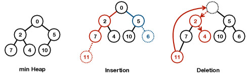
Figure 1. An example of min-heap and irregularity in the heap operations

However, it is non-trivial to exploit parallelism of the binary heap, and reason about the correctness given a parallel implementation. There are two key challenges that prevent us from fully taking advantage of the massive parallelism in many-core processors. Each update operation of the binary heap involves a tree walk. Different tree walks exhibit different control flow paths and the memory locality might be low. The control divergence and memory irregularity are two main performance hazards for GPU computing (Zhang et al., 2011). The two performance hazards need to be tackled before we can efficiently accelerate binary heap on GPUs. Moreover, as the parallel design gets complicated, it is not easy to reason about the correctness properties of the concrete implementation.

Existing work for parallelizing heap neither provide correctness guarantee nor take the GPU performance hazards into consideration. Among the research for parallelizing heap on CPUs, the work by Rao and Kumar (Nageshwara and Kumar, 1988) avoids locking the heap in its entirety, associates each node with a lock, and makes insertion updates top-down, such that the locking order of nodes prevents deadlock. Hunt et al. (Hunt et al., 1996) adopts the same fine grained locking mechanism, but makes insertion updates bottom up while maintaining a top-down lock order. The implementation by Hunt et al. alleviates the contention at the root node. However, neither of them formally reasons about the correctness of their implementation. Neither tackles the control divergence problem caused by random tree walks as it was not a problem for CPUs at the time when both works were published.

The closest related work to ours is by He and others (He et al., 2012) which is a GPU implementation of the binary heap. It is based on the idea presented by Deo and Prasad (Deo and Prasad, 1992) in 1992, which exploits the parallelism by increasing the node capacity in the heap. One node may contain $k$ keys ($k\geq$ 1). However, while it exploits intra-node parallelism, inter-node parallelism is not well exploited. It divides the heap into even and odd levels and uses barrier synchronization to make sure operations on two types of levels are never processed at the same time. It assumes all insertion/deletion updates progress at the same rate. Moreover, between every two consecutive barrier synchronization points, only one insertion or deletion request can be accepted, which severely limits the efficiency of its implementation on GPUs. Our implementation is shown to be much faster than the work by He et al.(He et al., 2012) (in Section 5).

In this work, we present a design of concurrent heap that is well-suited for many-core accelerators. Although our idea is implemented and evaluated on GPUs, it applies to other general purpose accelerator architecture with vector processing units. Further, we not only show that our design outperforms sequential CPU implementation and existing GPU implementation, but also prove that our concurrent heap is linearizable. Specifically, our contribution is summarized as follows:

1. We develop a generalized heap model. In our model, each node of the heap may contain multiple keys. This similar to the work by Deo and Prasad (Deo and Prasad, 1992). However, there are two key differences. First, assuming $k$ is the node capacity, Deo and Prasad (Deo and Prasad, 1992) only allow inserting/deleting exactly $k$ keys, while it is not uncommon that an application inserts/deletes less than or more than $k$ keys. We added support for partial insertion and deletion in our generalized model. Second, we exploit both intra-node parallelism and inter-node parallelism, the latter of which is not fully explored by Deo and Prasad (Deo and Prasad, 1992) or He et al. (He et al., 2012). Note that the benefit of having multiple keys in one node is multi-fold. It allows for intra-node parallelism, memory parallelism, local caching, and can alleviate control divergence since in a tree walk $k$ keys in the same node move along the same path.

2. We prove the linearizability of our implementation. We propose two types of heap implementations and prove both are linearizable. Linearizability is a strong correctness condition. A history of concurrent invocation and response events is linearizable if and only if some (valid) reordering of events yield a legal sequential history. We provide a model for describing the concurrent and sequential histories and for inserting linearization points. As far as we know, existing heap implementations on CPU (Hunt et al., 1996; Nageshwara and Kumar, 1988; Deo and Prasad, 1992) or GPU (He et al., 2012) do not have a formal reasoning about their correctness or linearizability condition.

3. We perform a comprehensive evaluation of the concurrent heap. We thoroughly evaluate our heap implementation and provide an enhanced understanding of the interplay between heap parameters and execution efficiency. We perform sensitivity analysis for heap node capacity, partial operation percentage, concurrent thread number, and initial heap utilization. We explore the difference between insertion and deletion performance. We also evaluate our implementation on real workloads, while most previous work use synthetic traces (Hunt et al., 1996; Nageshwara and Kumar, 1988; Deo and Prasad, 1992; He et al., 2012), as far as we know. We show that performance improvement could be up to 19.49 times compared with sequential CPU implementation, 2.11 times compared with the existing GPU implementation. We improve the single source shortest path algorithm by up to 123% and improve the performance of 0/1 knapsack by up to 1219%, which demonstrates the great potential of applying priority queue on GPU accelerators.

2. Background

2.1. Heap Data Structure

A heap data structure can be viewed as a binary tree and each node of the binary tree stores a key. Without loss of generation, we use the min-heap to describe our idea throughout the paper. The minimal key is stored at the root node. A node’s key is smaller than or equal to parent’s key. A heap is maintained using two basic operations: insert and delete-min.

During the insertion process, a key is inserted to an appropriate location such that the heap property is maintained. In a bottom-up insertion process, it places the key in the first empty leaf node, then repeats the following steps: compare a node’s key with its parent node’s key, if smaller, then swap itself with the parent node, otherwise, terminate. The bottom-up insertion algorithm is shown in Fig. 2 (a).

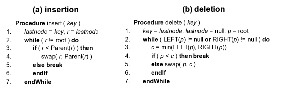
Figure 2. Insert and Delete in a sequential Heap

A delete-min procedure returns the minimal key in the heap. It removes the key at the root node and starts a “heapify” process to restore the min-heap property. To heapify, it moves the last leaf node to the root, and repeat the following steps: (1) compare the node p’s left child and right child (if there is any), (2) return the smaller of the two as $c$, and (3) if p’s key is larger than c’s key, swap the node c with the node p, otherwise, terminate. The algorithm is shown in Fig. 2 (b).

2.2. GPU Architecture

GPU is a type of many-core accelerator. It employs the single instruction multiple thread (SIMT) execution model. In order to take advantage of GPU, two fundamental factors need to be taken into consideration (Kumar et al., 2008; Moscovici et al., 2017): control divergence and memory locality.

In SIMT model, threads are organized into groups, each of which executes in lock-step manner. Each group is called a warp. The threads in the same warp can only be issued one instruction at one time. If threads in the same warp need to execute different instructions, the execution will be serialized. This is called control divergence.

During execution, the data must be fetched for all threads at each instruction. The warp cannot execute until the data operands of all its threads are ready. Memory parallelism needs to be exploited since data in physical memory is organized into large contiguous blocks. Data is fetched in the unit of memory blocks. If one memory references involves non-contiguous data access in multiple blocks, the warp needs to fetch multiple blocks. If one memory reference involves contiguous data access in memory, it will reduce the number of memory blocks that need to be fetched.

The SIMT model provides a limited set of synchronization primitives. Barrier synchronization is allowed for threads within CTA. A GPU kernel does not complete until all its threads have completed, which can be used as an implicit barrier among all threads. Although there is no provided lock intrinsics on GPUs, the atomic compare and swap (CAS) function is provided ,and can be used to implement synchronization primitives.

2.3. Linearizability

In concurrent programming, linearizability (Herlihy and Wing, 1990) is a strong condition which constrains the possible output of a set of interleaved operations. It is also a safety property that enables us to reason about the expected results from a concurrent system (Shavit and Taubenfeld, 2016). The execution of these operations results in a history, an ordered sequence of invocation and response events. The invocation refers to the event when an operation starts. The response refers to the event when operation completes.

A sequential history is the one that an invocation is always followed by a matching response, and a response event followed by another invocation. Alternatively, since in a sequential history operations do not overlap, we can consider as if an invocation and its matching response happen at the same time, and an operation takes immediate effect. There is no real concurrency in a sequential history. However, a sequential history is easy to reason about.

We say that the history $H$ as an ordered list of invocation and response events { ${e_{1},e_{2},...,e_{k}}$} is linearizable if there exists a re-ordering of the events such that (1) a correct sequential history can be generated, and (2) if the response of an operation $e_{i}$ precedes the invocation of another operation $e_{j}$, $res(e_{i})$ $<$ $inv(e_{j})$, then the operation $e_{i}$ precedes the operation $e_{j}$ in the reordered events. Typically linearization point is used to denote the time when an operation takes immediate effect between the invocation and response of one operation. Finding the right linearization points to construct a correct sequential history naturally meets the condition of (2).

3. Concurrent Heap Design

We exploit the parallelism of heap operations by allowing concurrent insert operations, INS, and delete operations, DEL, on different tree nodes. In the meantime, each node in the binary tree is extended to contain a batch of keys instead of only one. We refer to this proposed heap as the generalized heap throughout this paper. Our heap is well-suited for acceleration on GPUs. Parallelism exists within a batch of keys and the control divergence is reduce because all keys in the same batch move along the same path in the tree during tree traversals.

3.1. Generalized Heap

Each node in the generalized heap contains $k$ keys. Since the number of keys in the heap is not always a multiple of $k$ and an insertion or deletion may not be exactly $k$ keys, we use a partial buffer implementation. The partial buffer contains no more than $k-1$ keys . All the keys in the partial buffer should be larger than or equal to the keys in the root node so as to make sure the smallest $k$ keys are in the root node. We denote the $k$ keys in one heap node as a batch.

Like conventional heap, after each INS and DEL update on the generalized heap, the heap property needs to be preserved. Here, we formally define the generalized heap property:

1. Given any node $c$ in the generalized heap and its parent node $p$, the smallest key in $c$ is always larger than or equal to the largest key in $p$:

   $$\min\limits_{i=1..k}{node[c][i]}\geq\max\limits_{j=1..k}{node[p][j]}$$

2. Given any node $c$ in the generalized heap, the keys in $c$ are sorted in ascending order:

   $$\forall i\in[1,k):node[c][i]\leq node[c][i+1]$$

3. Given the partial buffer $b$ with size $s$, all the keys are sorted in ascending order and are larger than or equal to those in the root node $r$:

   $$\forall i\in[1,s):node[b][i]\leq node[b][i+1]$$

   $${node[b][1]}\geq{node[r][k-1]}$$

Note that the heap property for the conventional heap is a special case of the generalized heap property with $k$ = 1. When the batch of each node contains only one key, the generalized heap property 1 and 2 are still satisfied. The generalized heap property 3 does not apply since the partial buffer contains at most $k-1$ keys so there is no partial buffer in the conventional heap.

The most space efficient way to represent a generalized heap is using the array. Each entry of the array represents a single key and consecutive $k$ entries represent a node. Thus, the generalized heap can be represented as a linear array while the first $k$ entries are from the root node and the next $k$ entries are from the second node and so on. Therefore, array entries in the range of $[i*k,(i+1)*k-1]$ are from the $i$-th node in the generalized heap. An array representation allows an implicit binary tree representation of the generalized heap. Fig. 3 shows an example of the generalized heap in both array representation and binary tree representation. The partial buffer is stored separately.

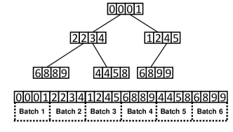
Figure 3. An example of the generalized heap

3.2. INS and DEL operations on the Generalized Heap

There are two basic operations for heap: DEL operation deletes the root node which contains the smallest $k$ keys from the heap and INS operation inserts new keys into the heap. We describe these two basic operations on the generalized heap.

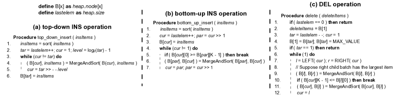
Figure 4. Pseudo Codes for INS and DEL operations on Generalized Heap

3.2.1. DEL Operation

The DEL operation on the generalized heap retrieves the $k$ keys from the root node. Since the root node is left empty, the generalized heap needs to be heapified to satisfy the generalized heap property. The pseudo code is shown in Fig. 4(c).

The DEL operation refills the root node with the keys from the last leaf node of the heap (line 1 - 5). Note that we will fill the last node with a MAX value to make sure the old keys in that node are covered. Then, we propagate the new values in root node down. During the propagation, DEL operation will perform the MergeAndSort operation on two child nodes $l$ and $r$ (line 9). Here we formally define the MergeAndSort operation between two batch of keys $a$ and $b$:

$$(batch[hi][1:k],batch[lo][1:k])=\textbf{MergeAndSort}(batch[a][1:k],batch[b][1:k])\textbf{ such that}$$

$$\forall i\in[1,k):batch[hi][i]\leq batch[hi][i+1]$$

$$\forall i\in[1,k):batch[lo][i]\leq batch[lo][i+1]$$

$$\max\limits_{i=1..k}{batch[hi][i]}\leq\min\limits_{j=1..k}{batch[lo][j]}$$

MergeAndSort operation returns two batches $hi$ and $lo$ with size $k$. $hi$ stores the $k$ smallest keys and $lo$ stores the $k$ largest keys.

The DEL operation places the $lo$ part back to the child node whose maximum key was larger (compared with the other child) before (line 9). In this example, let’s suppose it is the child node $r$. It can be proved that with such a placement policy, the generalized heap property on the sub-heap of $r$ will be maintained. The $hi$ part is placed into the child node $l$. Then, another MergeAndSort operation is applied to the current node and the child $l$ (line 11). The $k$ smallest of the merged result will stay in the current node, and the $k$ largest will propagate through sub-heap of $l$. The propagation ends until the generalized heap property is satisfied (line 10). An example of the DEL operation is shown in Fig. 5.

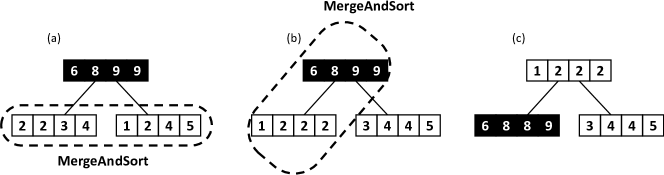
Figure 5. Example: Deletion for the generalized heap

3.2.2. INS Operation

The INS operation inserts new keys into the generalized heap. It grows the heap by adding a new node to the first empty node in the heap, we call this location the target node. Given the target node, a path from the root node to the target node can be found and we call it the insert path.

There are two possible directions for the propagation of the INS operation, which leads to two different types of INS operation: ① top-down INS, which starts from the root node and propagates down until it reaches the target node; ② bottom-up INS, which starts at the target node and propagates up until it reaches the root node or when the generalized heap property is satisfied in the middle of the heap.

Top-down INS operation

The top-down INS operation starts at the root node and propagates down to the bottom level of the heap. The propagation of the top-down INS operation follows the insert path, the MergeAndSort operation is performed between the new insert items and each node on the insert path until it reaches the target node. An example of the top-down INS operation is shown in Fig. 6 and the pseudo code is provided in Fig. 4(a).

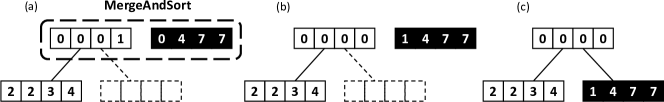
Figure 6. Example: Top-Down Insertion

Bottom-up INS operation

The bottom-up INS operation inserts new keys from the bottom of the heap to the root batch of the heap and still follows the corresponding insert path. The pseudo code is shown in Fig. 4(b). We first move the to-insert new keys to the target node (line 3). Since the generalized heap property may be violated, the MergeAndSort operation is performed between the nodes on the insert path and their parent nodes. The propagation keeps going along the insert path until it reaches the root batch or the generalized heap property is satisfied in the middle (line 5). An example of bottom-up INS is provided in Fig. 7.

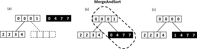
Figure 7. Example: Bottom-Up Insertion

Discussion

Compared to top-down INS operation, bottom-up INS operation may not need to traverse all the nodes on the insert path since the generalized heap property may be satisfied in the middle. Moreover, when concurrent INS and DEL operations are performed on the generalized heap, bottom-up INS operation can reduce the contention on the top levels of the heap. However, the bottom-up INS operation needs to pay attention to the potential deadlock problem caused by the opposite propagation directions of INS and DEL operations. We will discuss more about these concurrent INS and DEL operations in the following sections.

3.3. Concurrent Heap

In this section, we describe how DEL and INS operations can be performed concurrently on our parallel generalized heap. Our algorithms are inspired by the methods discussed in (Nageshwara and Kumar, 1988) and (Hunt et al., 1996) which introduced concurrent INS and DEL operations on a heap with $k=1$, with top-down INS and bottom-up INS operations respectively. In this paper, we call the concurrent heap with Top-Down INS operation the TD-INS/TD-DEL Heap and the one with Bottom-Up INS as BU-INS/TD-DEL Heap.

3.3.1. Lock Order for INS and DEL operations

In (Nageshwara and Kumar, 1988) and (Hunt et al., 1996), to support concurrent INS and DEL operations while ensuring correctness and avoiding deadlocks, a simple lock strategy is applied. Instead of locking the whole heap, each node of the heap is assigned a lock and only a small portion of the nodes are locked at one time. Our first implementation adopts this method. In Fig. 8, we show how we handle the locking order for both INS and DEL operations. The partial buffer is handled when the root node is locked, so that both the root node and the partial buffer is protected by the same lock. For all other nodes, each node has only one lock.

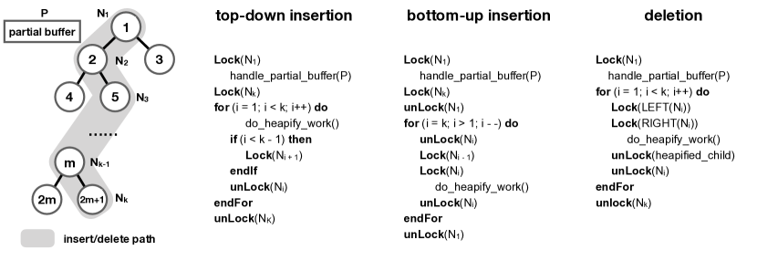
Figure 8. Lock Order for top-down INS, bottom-up INS and DEL operations

The top-down INS operation starts at the root node $N_{1}$ and propagates along the insert path $N_{1},N_{2},...,N_{k}$. It will do the heapify work of $N_{i}$ when it has locked $N_{i}$. After it finishes its work, it will lock $N_{i+1}$ before it unlocks $N_{i}$ which follows a parent-child locking order. Similarly, the bottom-up INS operation also follows the parent-child locking order. When the bottom-up INS is at $N_{i}$, it will release the lock on $N_{i}$ first, locks $N_{i-1}$ next and then locks $N_{i}$. Note that, in this case, the bottom-up INS operation does not lock any node after it releases $N_{i}$. The DEL operation needs to lock more nodes during its propagation. When it is at $N_{i}$ and $N_{i}$ is locked, it then locks its two child nodes and do the heapify work. After the work is done, it unlocks the child node that is already heapified and then $N_{i}$. In this way, both INS and DEL operations follow the parent-child order so that no deadlock could happen.

Each node of the heap is associated with a multi-state lock. This multi-state lock has multiple states which can indicate the status of each node. The multi-state lock for top-down INS and bottom-up INS operations have different states. We describe the difference in the following sections.

We implement the multi-state lock using atomicCAS. Atomic operations are well optimized on GPUs (Corporation, 2010) which makes it a straightforward choice to implement the multi-state lock.

3.3.2. TD-INS/TD-DEL Heap

Our TD-INS/TD-DEL heap implements top-down insertions and top-down deletions, using the locking order as described in Fig. 8. We let the multi-state lock have four different states: AVAIL indicates that the node is available; INUSE means that the node is acquired by another operation; To lock a node, the state of that node changes from AVAIL to INUSE. A node with state TARGET represents that the node is the target node of a insert operation; The state of a node is changed to MAKRED only when the target node is needed by a delete operation for insertion and deletion cooperation. Finite State Automata is shown in Fig. 9.

The INS and DEL operations can cooperate to speedup the propagation(Nageshwara and Kumar, 1988). When the DEL operation needs to fill the root node, if there is an INS operation that is being in progress. The DEL operation does not need to wait until the last leaf node to be ready (if it is not ready and if it is the target node of an in-progress insertion), it can fill the root node with the keys from the INS operation.

The DEL operation changes the state of the last node from TARGET to MARKED. to let the INS operation know that a DEL operation is asking for the insert keys. When the INS operation finds that the state of the target node is MAKRED, it moves the insert keys to the root node and terminate. The DEL operation can then continue and use those keys in the root node for propagation.

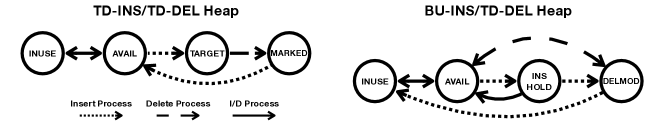
Figure 9. FSA of TD-INS/TD-DEL Heap and BU-INS/TD-DEL Heap

To handle partial batch insertion, we acquire the partial buffer at the time when we hold the root node. Since only one operation can work on the same node, this can make sure that no two operations can work on the partial buffer at the same time. Then we apply the MergeAndSort operation between the insert keys and the partial buffer. We check if the partial buffer have enough space to contain those new keys. If so, we perform another MergeAndSort operation between the partial buffer and the root node to satisfy the generalized heap property 3. If not, we obtain the k smallest keys from the MergeAndSort result as a full batch and propagate it down through the root node, while leaving the rest keys in the partial buffer.

For DEL operation, we only consider deleting the items from the partial buffer when the total number of keys is less than a full batch, in another word, all heap nodes are empty. This is because based on the generalized heap property 3, the root node always have the smallest keys in the heap. Although allowing partial batch insertion will cause extra overhead, however, the inserted keys in the partial buffer do not need to propagate into the heap immediately until the partial buffer is overflown. In this way, we still gain the benefit of memory locality and the intra-node parallelism.

We show the pseudo code of INS and DEL operations on the TD-INS/TD-DEL Heap in Fig. 10.

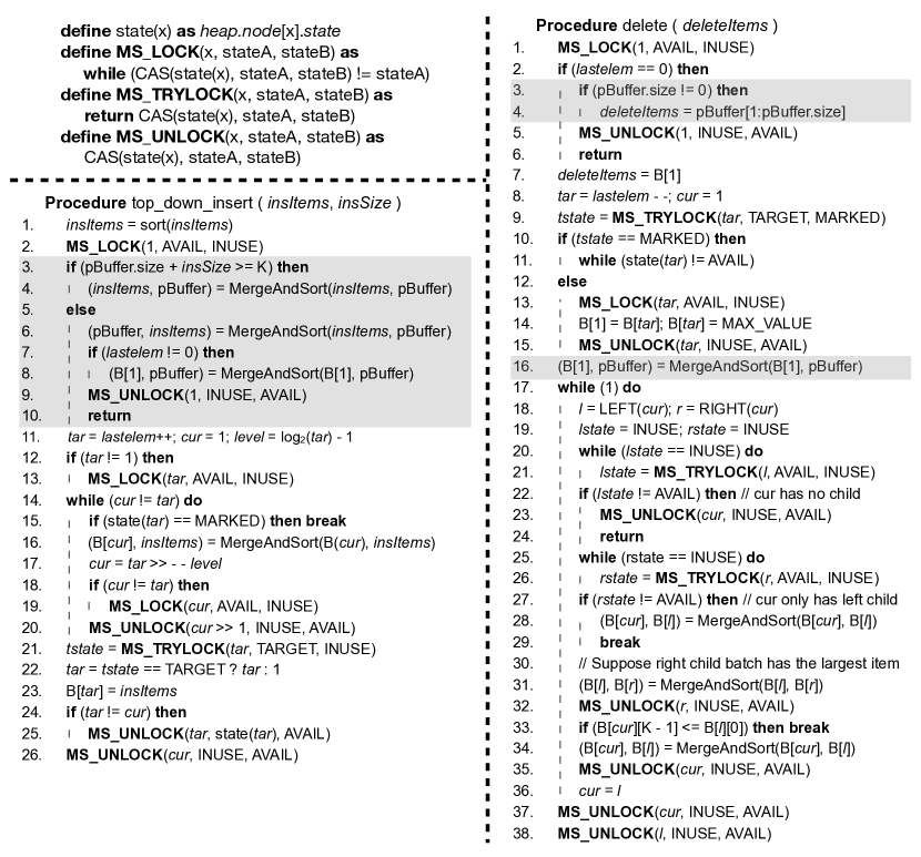
Figure 10. Pseudo Codes for TD-INS/TD-DEL Heap Operations

3.3.3. Linearizability of TD-ins/TD-del Heap

We show that the heap with top-down insertion and top-down deletion (TD-Ins/TD-Del) is linearizable.

In order to reason about the linearizability, we need to define our notations. An ins or del operation takes a certain amount of time to complete. We denote the time an operation is invoked as the invocation time, the time when an operation is completed as the response time. A history includes an ordered list of invocation and response events (ordered with respect to time).

Our TD-Ins/TD-Del implementation uses fine-grained locks that each node is associated with a lock. We denote the time a thread acquires the lock of a node as acquire time and the time a thread release the lock of a node as release time.

We denote an operation with a 4-tuple followed by two parameters $op[s,ac,re,t](x)T$. The symbol $op$ is the type of the operation, ins or del; $s$ is the invocation time, $t$ is the response time; $ac$ refers to acquire time of a node of interest; $re$ refers to release of the same node; $x$ is the parameter of the operation, if the operation is insertion, it means insert $x$ into the heap, if the operation is deletion, it means $x$ is returned; $T$ refers to the thread id. Note that both $ac$ and $re$ are within the time interval $s$ and $t$, and that $ac<re$.

To prove linearizability, we need to show that for any given history H, we can find a correct sequential history S based on a valid reordering of invocation and response events in H. Here the term “valid reordering” refers to the case when there are two operations $e_{0}$ and $e_{1}$ in H, if the response time of $e_{0}$ is before the invocation time of $e_{1}$, $e_{0}$ will proceed $e_{1}$ in the sequential history.

To prove such a sequential history exist, we prove the following lemma first.

Lemma 3.1.

No two threads can work on the same heap node simultaneously.

Proof.

According to our implementation, if a thread T has acquired the node $B$ which means the T has changed $B$’s state to INUSE, then no other thread can acquire $B$ until T releases it. ∎

We denote a history H with n operations as $H$ = { $op^{H}_{i}$($s_{i}$, $acR_{i}$, $reR_{i}$, $t_{i}$) $x^{H}_{i}$ $T^{H}_{i}$ — $1\leq i\leq n$ } . Here $acR$ and $reR$ respectively refer to the acquire and release of the lock for the root node in the heap. In our notation, the history $H$ is an ordered list such that its operations are ordered with respect to the time the root node is released. Since each operation in TD-INS/TD-DEL heap needs to acquire the root at its first step in fig. 10, and based on Lemma 3.1, only one thread can successfully acquire root node at one time. Thus for two operations $op^{H}_{u}$($s_{u}$, $acR_{u}$, $reR_{u}$, $t_{u}$ ) $x^{H}_{u}$ $T^{H}_{u}$, and $op^{H}_{v}$($s_{v}$, $acR_{v}$, $reR_{v}$, $t_{v}$) $x^{H}_{v}$ $T^{H}_{v}$, we have $u<v$ if and only $reR_{u}<acR_{v}$.

Theorem 3.2.

The TD-INS/TD-DEL heap is linearizable.

Proof.

We show that we can construct a sequential history S given any H. To construct the sequential history, we first construct a list of linearization points { $N_{i}$ — i = 1 to n } such that $acR_{i}$ $<$ $N_{i}$ $<$ $reR_{i}$. Simply put, $N_{i}$ is an arbitrary time point between every pair of events that acquire and release the root node. An example of setting linearization point is shown in Fig. 11.

An operation appear to occur instantaneously at its linearization point. A linearization point has to be between the invocation time and response time for an operation, since acquiring and releasing root is a step within every update in TD-Ins/TD-Del heap, the $N_{i}$ time points we set here is naturally between invocation and response time.

Next we construct a sequential history as

$S$ = { $op^{S}_{i}$($N_{i}$) $x^{S}_{i}$ $T^{S}_{i}$ — $1\leq i\leq n$ }

We set a one-to-one correspondence between the i-th operation $op^{H}_{i}$($s_{i}$, $acR_{i}$, $reR_{i}$, $t_{i}$) $x^{H}_{i}$ $T^{H}_{i}$ in H and the i-th operation $op^{S}_{i}$($N_{i}$) $x^{S}_{i}$ $T^{S}_{i}$ in S. We set $T^{S}_{i}=T^{H}_{i}$ and $op^{S}_{i}=op^{H}_{i}$. For all insert operations, we set $x^{S}_{i}=x^{H}_{i}$, which means we insert the same key items for the corresponding operation in S. Next we prove that $x^{S}_{i}=x^{H}_{i}$ for every delete update, which means every delete operation in S returns the same value as its corresponding delete operation in H.

Assume that when the m-th operation in H releases root node at time $reR_{m}$, the heap value is $Heap^{H}_{m}$, its set of keys are denoted as $set(Heap^{H}_{m})$, and its root node is denoted as $root(Heap^{H}_{m})$. Similarly, at the time $N_{m}$ of the m-th operation in S, assume the heap value is $Heap^{S}_{m}$, its set of keys are denoted as $set(Heap^{S}_{m})$, and its root node is denoted as $root(Heap^{S}_{m})$. We prove two properties:

1. $set(Heap^{H}_{i})=set(Heap^{S}_{i})$, $1\leq i\leq m$

2. $root(Heap^{H}_{i})=min(set(Heap^{H}_{i}))$ and $root(Heap^{S}_{i})=min(set(Heap^{S}_{i}))$, $1\leq i\leq m$

We prove properties L1 and L2 by induction. Initially we have $H_{0}$ which is an empty history, and a heap value $Heap^{H}_{0}$. We set $S_{0}$ empty and set $Heap^{S}_{0}$ to be the same as $Heap^{H}_{0}$. Properties L1 and L2 are satisfied for the initial heap.

Assume at the time point $reR_{k}$ in H and at the time point $N_{k}$ in S, properties L1 and L2 hold. We just need to prove for the time point $reR_{k+1}$ in H and the time point $N_{k+1}$ in S, properties L1 and L2 hold as well. There are two cases.

Case I – the (k+1)-th operation in H is an insertion: $ins^{H}_{k+1}(s_{k+1},acR_{k+1},reR_{k+1},t_{k+1})x^{H}_{k+1}T^{H}_{k+1}$. At the time $reR_{k+1}$, since when a thread releases a root node in our implementation, the new item $x^{H}_{k+1}$ is already merged with the original root and the smaller item of the merged result is kept in root while the larger item may or may not propagate down the heap. Therefore the root node should contain the smallest item after taking the new item $x^{H}_{k+1}$ into consideration. Formally, $set(Heap^{H}_{k+1})=set(Heap^{H}_{k+1})\bigcup x^{H}_{k+1}$ and $root(Heap^{H}_{k+1})=min(set(Heap^{H}_{k+1}))$.

In the sequential history, since we also set (k+1)-th operation as insert update at time $N_{k+1}$, the operation is $ins^{S}_{k+1}(N_{k+1})x^{S}_{k+1}T^{H}_{k+1}$, where $x^{S}_{k+1}=x^{H}_{k+1}$. In sequential history, the insertion incurs as if instantaneously, thus $set(Heap^{S}_{k+1})=set(Heap^{S}_{k})\bigcup x^{H}_{k+1}$ and $root(Heap^{S}_{k+1})=min(set(Heap^{S}_{k+1}))$. Thus $set(Heap^{H}_{k+1})=set(Heap^{S}_{k+1})$, $root(Heap^{H}_{k+1})=min(set(Heap^{H}_{k+1}))$ and $root(Heap^{S}_{k+1})=min(set(Heap^{S}_{k+1}))$. Properties L1 and L2 hold.

Case II – If the (k+1)-th operation in H is a deletion, $del^{H}_{k+1}(s_{k+1},acR_{k+1},reR_{k+1},t_{k+1})x^{H}_{k+1}T^{H}_{k+1}$. In our implementation, the deletion removes the root which is $min(set(Heap^{H}_{k}))$ and re-heapifies the heap. It does not release root until root node is updated to the smallest of the remaining items, thus at the time point $reR_{k+1}$, $root(Heap^{H}_{k+1})=$ $min(set(Heap^{H}_{k})-min(set(Heap^{H}_{k})))$.

In the sequential history, we set a delete operation at the time point $N_{k+1}$, as if the delete update happens instantaneously. Then the delete update returns $min(set(Heap^{S}_{k}))$ which is the same as $min(set(Heap^{H}_{k})))$, and in the meantime, root node will be updated to $min(set(Heap^{S}_{k})-min(set(Heap^{S}_{k})))$ which is also the same as the root of $Heap^{H}_{k+1}$ as described above. Thus properties L1 and L2 still hold.

Thus we have successfully constructd a sequential history S from any given history H. Therefore, the TD-INS/TD-DEL heap is linearizable.

∎

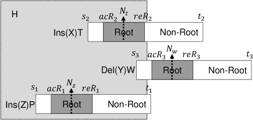
Figure 11. Example: set up of linearization points for TD-INS/TD-DEL heap operation history

3.3.4. BU-INS/TD-DEL Heap

To reduce the contention on the root node of top-down INS operations, Hunts et.al (Hunt et al., 1996) proposed a mechanism that does bottom-up INS operations while solving the potential deadlocks from opposite propagation direction. It allows the insert thread temporarily releases the control of the insert items and a tag is used to store the $pid$ of the thread that modifies the insert items. Here we use a similar method but does not need to store the $pid$.

The multi-state lock used in BU-INS/TD-DEL Heap have four different states. INUSE and AVAIL are the same as the ones used in TD-INS/TD-DEL Heap. Since the insert operation may temporarily release the control of its node, so it uses the state to tell whether the node has been modified by the time it releases the node. It changes the state of the node from INUSE to INSHOLD when it releases the node. When the insert operation acquire the node again, if it finds that the state is no longer INSHOLD, this means one or more delete operations have modified this batch and the insert operation can skip this batch since the delete operation makes sure the sub-heap has satisfied the generalized heap property. On the contrary, the delete operation which acquires the node from INSHOLD to INUSE will change the state to DELMOD when releasing the node.

We show the FSA of the BU-INS/TD-DEL Heap in Fig. 9. The pseudo codes of the concurrent insert and delete operations in bottom-up manner are shown in Fig. 12.

When an insert operation acquires the temporarily released node, there are three possible cases for the new state with that node:

1. INSHOLD: the insert operation holds the batch successfully and the MergeAndSort operation can be performed with the parent batch.

2. DELMOD: the batch has been modified by one or more delete operations, the insert operation can move to the parent batch.

3. INUSE: some other operations are using this batch

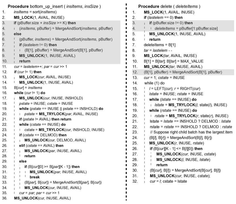
Figure 12. Concurrent Insertion and Deletion with partial batch in Bottom-Up Mode

The state of the parent node may also be changed. If the state is not AVAIL or INUSE, this means a delete operation has already deleted the parent node and the insert operation can terminate.

Partial buffer is handled at the beginning of each operation when it locks the root node. For both INS and DEL operations, the part for handling the partial buffer is exactly the same as the one we showed in Section 3.3.2 so as to make sure generalized heap property 3 is satisfied.

3.3.5. Linearizability of BU-ins/TD-del Heap

Now we show that the BU-INS/TD-DEL Heap is linearizable. Note that we will use the same notations that we have defined previously in Section 3.3.3. We use the notation $ins_{i}^{H}(s_{i},acL_{i},reL_{i},t_{i})x_{i}^{H}T_{i}^{H}$ for INS operation $i$ and $del_{j}^{H}(s_{j},acR_{j},reR_{j},t_{j})x_{j}^{H}T_{j}^{H}$ for DEL operation $j$. Here $acL$ and $reL$ respectively refer to the acquire and release for the last locked node in a bottom-up INS operation. This last locked node may or may not be the root node, since the generalized heap property may be satisfied in the middle of a bottom-up $INS$ update.

We denote a history H with n operations as $H=\{op_{i}^{H}(s_{i},ac_{i},re_{i},t_{i})x_{i}^{H}T_{i}^{H}|1\leq i\leq n\}$ while $ac_{i}$ and $re_{i}$ can be either $acL_{i}$ and $reL_{i}$ for INS, or $acR_{i}$ and $reR_{i}$ (R is for root ) for DEL. The operations in H are ordered with respect to the time $re_{i}$ ( either when INS release the last locked node or when DEL release the root node ). It is possible that the time $re_{u}$ and $re_{v}$ are the same for two operations $op_{u}$ and $op_{v}$. In this case, an arbitrary order can be chosen. Thus for two operations $op^{H}_{u}$($s_{u}$, $ac_{u}$, $re_{u}$, $t_{u}$ ) $x^{H}_{u}$ $T^{H}_{u}$, and $op^{H}_{v}$($s_{v}$, $ac_{v}$, $re_{v}$, $t_{v}$) $x^{H}_{v}$ $T^{H}_{v}$, we have ${u}<{v}$ when $re_{u}<re_{v}$ or $re_{u}==re_{v}$.

Lemma 3.3.

Given a delete operation $del_{i}^{H}(s_{i},acR_{i},reR_{i},t_{i})x_{i}^{H}T_{i}^{H}$ and an insert operation $ins_{j}^{H}$($s_{j}$, $acL_{j}$, $reL_{j}$, $t_{j}$)$x_{j}^{H}T_{j}^{H}$ that $[acL_{j},reL_{j}]\cap[acR_{i},reR_{i}]$ $\neq\emptyset$, then $x_{i}^{H}\leq x_{j}^{H}$

Proof.

Based on Lemma 3.1 and the condition $[acL_{j},reL_{j}]\cap[acR_{i},reR_{i}]$ $\neq\emptyset$, we know that the last locked node of the insert operation is not the root node. Thus we can derive that $min(x_{j}^{H})\geq max(x_{i}^{H})$ which indicates that $x_{i}^{H}\leq x_{j}^{H}$. ∎

Theorem 3.4.

The BU-INS/TD-DEL heap is linearizable.

Proof.

We show that we can construct a sequential history S given any H. We construct a list of linearization points { $N_{i}$ — i = 1 to n } such that $acR_{i}$ $<$ $N_{i}$ $<$ $reR_{i}$ if the i-th operation is DEL, or $acL_{i}$ $<$ $N_{i}$ $<$ $reL_{i}$ if the i-th operation is INS. We pick $N_{i}$ as an arbitrary time point between the provided time range. We construct the sequential history $S$ = { $op^{S}_{i}$($N_{i}$) $x^{S}_{i}$ $T^{S}_{i}$ — $1\leq i\leq n$ } based on the linearization points. Each operation $op^{H}_{i}$ in S corresponds to an operation $op^{S}_{i}$ in H.

Like what we did in Section 3.3.3, we set $x^{S}_{i}=x^{H}_{i}$ if the i-th operation is INS. We will prove that $x^{S}_{j}=x^{H}_{j}$ if the j-th operation is DEL. We prove by induction. Initially we have an empty history $H_{0}$ and the heap value $Heap^{H}_{0}$. We set $S_{0}$ empty and set $Heap^{S}_{0}$ to be the same as $Heap^{H}_{0}$. At the beginning, we perform a (dummy) deletion in H and also a (dummy) deletion in S, both DEL return the same result. The dummy deletion in H completes before any real operation starts. The heap value for S and for H after the dummy deletion will be be the same.

Assume that $x^{S}_{k}=x^{H}_{k}$ at the time $re_{k}$ in H and at $N_{k}$ in S while the k-th operation in H is a delete operation $del^{H}_{k}$ and the k-th operation in S is also a delete operation $del^{S}_{k}$. Additionally, $set(Heap^{S}_{k})=set(Heap^{H}_{k})$, where $Heap^{S}_{k}$ is the heap value at the time $N_{k}$ in S, $Heap^{H}_{k}$ is not necessarily the heap value at the time $reR_{k}$ in H, rather, it is the set of keys that are contributed by all preceding insertion/deletion in H’s ordered list (note that the operations in H are already ordered, see the beginning of Section 3.3.5). Let the next delete update in H be the (k+m)-th operation $op^{H}_{k+m}$. If we prove that at the time point $re_{k+m}$ in H and $N_{k+m}$ in S with $m\geq 1$, both delete operations return the same value, that is $x^{S}_{k+m}=x^{H}_{k+m}$, and $set(Heap^{S}_{k+m})=set(Heap^{H}_{k+m})$, then we prove that all matching delete operations in S and H return the same value by induction.

In the concurrent history $H$, between time point $reR_{k}$ and $reR_{k+m}$, there are $m-1$ concurrent operations and these operations are all insert operations. Among all these m - 1 insert operations, we let $I^{H}$ be a set of insert operations such that

$I^{H}$ = {$ins_{i}^{H}(s_{i},acL_{i},reL_{i},t_{i})x_{i}^{H}T_{i}^{H}$ — $k<i<k+m$, $(acL_{i},reL_{i})$ $\cap(acR_{k+m},reR_{k+m})$ $\neq\emptyset$}

We let the set $I^{\prime}$ be the insert operations from these $m-1$ operations but not in $I$. The difference between $I$ and $I^{\prime}$ is that all $I^{\prime}$ operations complete before $op^{H}_{k+m}$, while $I$ operations might overlap with $op^{H}_{k+m}$. If we consider the inserted keys contributed by I’ as $X^{I^{\prime}}=\bigcup_{i\in I^{\prime}}x^{H}_{i}$. The set of keys in the heap would be $X^{I^{\prime}}\cup Heap^{H}_{k}$ if none of the operations in I has taken effect, the minimum would be $min(X^{I^{\prime}}\cup Heap^{H}_{k})$.

Let $X^{I}=\bigcup_{j\in I}x^{H}_{j}$, it is not difficult to show that $min(X^{I^{\prime}}\cup Heap^{H}_{k})=min(X^{I^{\prime}}\cup X^{I}\cup Heap^{H}_{k})$. According to Lemma 3.3, for any insertion $i$ in $I$, since its (acL, reL) interval overlaps with the root acquiring and releasing interval for $del^{H}_{k+m}$, we know that the last node locked by operation i cannot be the root, and thus the inserted value $x^{S}_{i},i\in I$ cannot be smaller than the root node. That is $x^{S}_{i}\geq min(X^{I^{\prime}}\cup Heap^{H}_{k})$ for any $i\in I$. Therefore, $min(X^{I^{\prime}}\cup Heap^{H}_{k})=min(X^{I^{\prime}}\cup X^{I}\cup Heap^{H}_{k})$ is proved. The implication is that regardless if any operation or all operations in the set I complete, $op^{H}_{k+m}$ will always return $min(X^{I^{\prime}}\cup X^{I}\cup Heap^{H}_{k})$ which is $min(\bigcup_{k<i<k+m}x^{H}_{i}\cup Heap^{H}_{k})$.

In the sequential history $S$, there are $m-1$ insert operations between time point $N_{k}$ and $N_{k+m}$. The heap should include the set of keys that are in $Heap^{S}_{k}$ and also $x^{S}_{i}$ ($k<i<k+m$). Thus $op^{H}_{k+m}$ returns $min(\bigcup_{k<i<k+m}x^{S}_{i}\cup Heap^{S}_{k})$.

Since $set(Heap^{S}_{k})=set(Heap^{H}_{k})$ and all matching insertion operations use the same parameter value for H and S, both $op^{H}_{k+m}$ and $op^{S}_{k+m}$ return the same value. Note that it is trivial to prove that $set(Heap^{H}_{k+m})=set(Heap^{S}_{k+m})$

Thus we have successfully constructed a sequential history S from any given history H. Therefore, the BU-INS/TD-DEL heap is linearizable

∎

4. Implementation

The building blocks of the generalized heap include the sorting operation, the MergeAndSort operation, and the multi-state lock that we introduced in Section 3.3.1. We use parallel bitonic sorting algorithm for local sorting operation within a thread block and merge-path(Green et al., 2012) algorithm for the MergeAndSort operation. We introduce optimization to eliminate redundant MergeAndSort operations and enable an early stop mechanism to reduce the total computation load and alleviate the contention on the locks.

In our implementation, threads in one thread block work together for one INS and DEL operation. We choose thread-block-level operation since barrier synchronization is provided within a thread block while no built-in inter-CTA synchronization is provided and the overhead for synchronization between all thread blocks is high.

Besides, threads within the same thread block have access to the same shared memory space, which can increase data reuse during propagation. We load frequently used items into the shared memory. Using thread-block-level INS and DEL operations can also benefit from memory coalescing. The items in the same node are placed continuously in the memory so that threads within the warp can achieve maximum memory coalescing. Also, the multi-state lock is a thread-block-level lock which is safer than a thread-level lock since a thread-level lock may cause deadlock due to desynchronization within a warp (Wong et al., 2010).

4.1. Sorting Operation

The INS operations sorts the to-insert items before the propagation starts. To perform sorting, these to-insert items are loaded to the shared memory for efficient data access and movement. In our generalized heap implementation, the number of to-insert items for one insert operation is limited by the size of the shared memory per thread block (no more than 1K pairs in our case). We choose parallel bitonic sorting algorithm as it can be adopted for our thread-block-level operations well.

Bitonic sorting is a comparison-based sorting algorithm. Other efficient non-comparison based GPU sorting algorithms (e.g. parallel radix sort) require types to have the same lexicographical order as integers. This not only limits the practical use of the sorting algorithms to only numeric types like $int$ or $float$ but also the sorting complexity of which is based on the size of the key (length of the data). As we mentioned before, in our parallel generalized heap, the number of the to-insert items is usually small, which means the size of the key can dominant the sorting efficiency. Parallel bitonic sorting algorithm’s complexity depends on the number of input elements which makes it more suitable for our case.

4.2. MergeAndSort Operation

In both INS and DEL operations, we perform the MergeAndSort operations frequently during the heapify process. This can be optimized thanks to the generalized heap property 2 that the keys in a node are already sorted. Instead of directly sorting the keys that need to be merged, performing a MergeAndSort operation on those sorted nodes will be more time efficient.

In our parallel generalized heap implementation, the number of items in a node is small and we also load the data into the shared memory. Here we use the GPU merge-path algorithm (Green et al., 2012), which merges two already sorted sequences. The main advantage of the merge-path method is that it can assign workload evenly to threads. It has low-latency communication and high-bandwidth shared memory usage which our implementation can benefit from a lot. Detailed description and complexity analysis of the GPU merge-path algorithm can be found in (Green et al., 2012).

4.3. Optimizations

To improve the performance of concurrent INS and DEL operations, we apply the following optimizations.

Remove Redundant MergeAndSort Operations

MergeAndSort operation is the major overhead of heap operations. It is used frequently to make sure that the generalized heap satisfies generalized heap property. In our implementation, we compare the keys in the nodes and then decide if a MergeAndSort operation is necessary. When the largest keys in a node is smaller than the smallest key in the other, instead of performing the MergeAndSort operation, we simply swap the two nodes which is much more efficient. This optimization reduces the number of MergeAndSort operations within every insert and delete operation.

Early Stop

This optimization is similar to what we do in a conventional heap. The INS and DEL operations will terminate once the generalized heap property is satisfied. For our generalized heap, Early Stop can happen for all operations except for top-down INS which has to bring the to-insert items to the target node that locates at the bottom of the heap. Thus it has to traverse all levels of the generalized heap.

Bit-Reversal Permutation

The INS operation needs to decide the target node and two consecutive INS operations may select the two target nodes with the same parent. In this case, the insert path from the root node to the target nodes are highly overlapped which can increase the contention between the two INS operations. We apply the bit-reversal permutation(Hunt et al., 1996) that makes sure for any two consecutive INS operations, the two insert paths have no common nodes except the root node. Consecutive DEL operation also select the last batch in the heap following the bit-reversal permutation like INS operation, but in the reversed order.

5. Evaluation

5.1. Experiment Setup

We perform our experiments on an NVIDIA TITAN X GPU with an Intel Xeon E5-2620 CPU with 2.1GHz working frequency. The TITAN X GPU has 28 streaming multi-processors (SMs) with 128 cores, for a total of 3584 cores. Every thread block has 48 KB of shared memory and 64K available registers. The maximal number of active threads is 1K per thread block and 2K per SM.

We evaluate our parallel heap from six different perspectives:

• We compare our concurrent heap implementation with a sequential CPU heap and a previous GPU Heap (He et al., 2012). We use input workloads with different heap access patterns.

• We vary the number of the number of thread blocks to evaluate the impact of contention levels and the scalabiltiy. The number of threads affects the number of active ins or del operations.

• We perform sensitivity analysis with respect to heap node capacity K, the type of operation ins or del, and thread block size.

• We evaluate how inserting partial batches would influence the heap performance by varying the percentage of partial batch operations.

• We test the concurrent ins and del performance under different heap utilization which means the heap is initialized with different number of pre-inserted keys.

• We apply our parallel heap to two real world applications which are single source shortest path (sssp) and 0/1 knapsack problem.

5.2. Concurrent Heap v.s. Sequential Heap

We use the GPU parallel heap implementation by He, Deo, and Prasad (He et al., 2012) as our GPU baseline. We refer to this implementation as parallel synchronous heap or in short, P-Sync Heap. We use the C++ STL priority queue library as the sequential CPU heap which we refer to as the STL Heap. Note that INS operation of the P-Sync Heap is top-down, while it is bottom-up for STL Heap.

We evaluate the performance of inserting 512M keys into an empty heap and then deleting all these 512M keys from the heap. We use different types of input keys which are ① randomized 32-bit int keys ② 32-bit int keys sorted in ascending order ③ 32-bit int keys sorted in descending order. The results are shown in Table 1.

Our concurrent heap has an average 16.59X speedup compared to the STL Heap and 2.03X speedup compared to P-Sync Heap. We observe the best performance when the input keys are sorted in ascending order in all cases. For STL Heap and BU-INS/TD-DEL Heap, it is because the INS operations only need to place the insert keys at the target node without traversing the entire heap. For P-Sync Heap and TD-INS/TD-DEL Heap, although INS operations start from the root node, we still gain the benefit of the keys sorted in ascending order as it avoids the overhead of unnecessary merging operations along the insert path.

Both TD-INS/TD-DEL Heap and BU-INS/TD-DEL Heap are faster than P-Sync Heap. This is because we can support concurrent INS or DEL at the same level of the heap while for P-Sync Heap, only one INS or DEL can work on the same level which exhibits with a lower inter-node parallelism. In later experiments, we will use randomized 32-bit keys for all INS and DEL operations performance evaluation except for the real world applications.

Table 1. Heap performance on CPU v.s. GPU

Method	random	descend	ascend
STL Heap	1,959,550	1,898,015	1,214,906
P-sync Heap	209,648	205,761	201,66
TD-INS/TD-DEL Heap	112,090	100,163	99,082
BU-INS/TD-DEL Heap	104,417	97,593	96,247

*Thread block number: 128, thread block size: 512,
K: 1024, time unit: milli-second (ms), keys: 512M

Figure 13. Heap performance w.r.t thread block numbers

5.3. Impact of Thread Number

We evaluate the performance of top-down insertion update, bottom-up insertion update, and deletion update respectively by varying the number of thread blocks. The more thread blocks, the more concurrency we can gain, and also the more contention on the heap. We fix all other parameters, with thread block size = 512 and batch size = 1024. We test the performance of inserting 512M random 32-bit keys into an empty heap for insertion-only experiments, and deleting 512M keys from a full heap for deletion-only experiemnt. We show the results in Fig. 13.

The performance of both ins and del operations become better when the number of thread blocks is increased since more concurrency can be obtained. However, the benefit from concurrency is restricted when the thread block number keeps increasing since more thread blocks also means more contention on the heap nodes.

The del operation always needs much more time than the ins operations especially when the thread block number is large which with an average 2.6X slow down. This is because del operation needs to hold both parent node and its two child nodes and performing at most two MergeAndSort operations when updating keys on each level of the heap while ins operation needs only one.

When comparing top-down ins with bottom-up ins operations. We see that bottom-up ins always has a better performance since it causes less contention on the root node of the heap and it may not need to traverse all the nodes on the insert path (the heap property may be satisfied in the middle).

5.4. Impact of Heap Node Capacity

Fig. 17 shows how ins and del performance is influenced by heap node capacity. Due to the limits in shared memory size per thread block, the maximum batch size we used is 1K. Also, the maximum number of thread block size depends on the batch size, since it does not make sense to have more than one thread handling one key in MergeAndSort operations. We test the performance by inserting 512M keys to an empty heap and deleting 512M keys from a full heap.

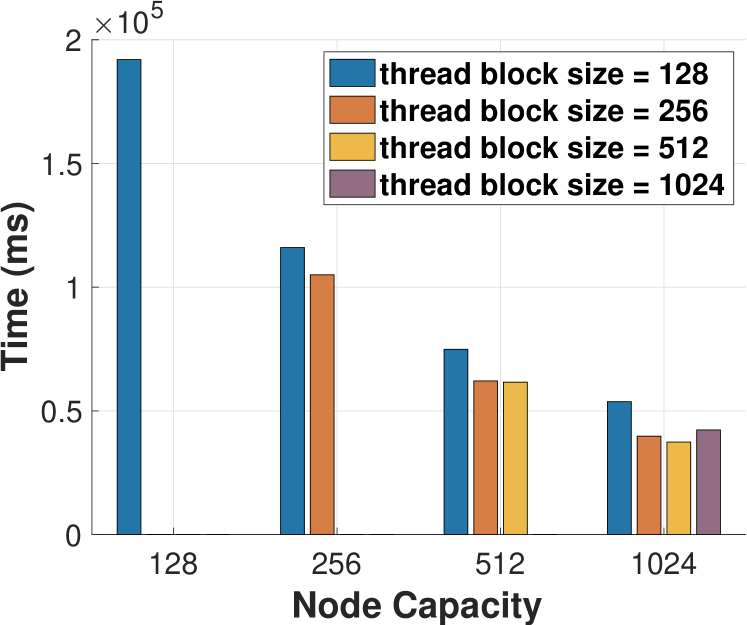
Figure 14. top-down ins operations

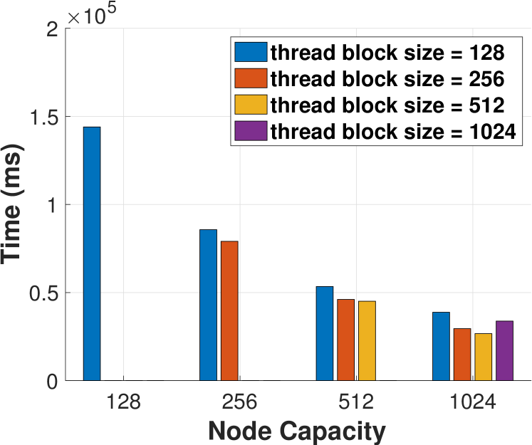
Figure 15. bottom-up ins operations

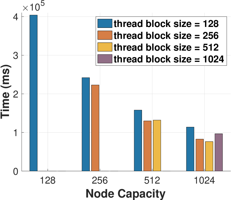
Figure 16. del operations

Figure 17. Performance of Inserting and Deleting 512M Keys w.r.t Node Capacity and Thread Block Size

When thread block size is the same, for both ins and del, we can observe that the performance becomes better when we use a larger node capacity. Using a larger node capacity means that with the same number of keys, the depth of the heap is reduced. If the node capacity is doubled then the level of the heap is reduced by one which leads to fewer MergeAndSort operations and tree walks. Also a larger node capacity can provide more intra-node parallelism.

In Fig. 17, it also shows that it is not always good to increase the thread block size because large thread block size can increase the overhead of synchronization within a thread block. Among all these configurations, we choose one with thread block size 512 and batch size 1024 for later experiments since it has the best performance for both ins and del operations.

5.5. Impact of Initial Heap Utilization

We control the initial heap size by pre-inserting a certain number of keys, for instance, to achieve a initial 10-level heap, we need to insert $batchSize*2^{10}$ keys. In this experiment, every thread performs one ins and one del, which we call an ins-del pair. Since the number of thread blocks is fixed and at most such number of ins could happens at the same time, so the heap level is also fixed only if the initial heap level is higher than a certain number. In our experiment, we use 128 thread blocks and each thread block will perform 2K ins-del pairs with a total 256K pairs.

In Fig. 19, we show the heap performance with respect to different initial heap size from a 6-level heap with 64K items to a 18-level heap with 256M items. We can observe that when the initial heap utilization is increased, these ins-del pairs need more time to finish. Both ins and del may traverse more levels of the heap and perform more MergeAndSort operations. Operations on BU-Heap have a better performance since bottom-up ins still has the benefit of stopping tree traversals earlier.

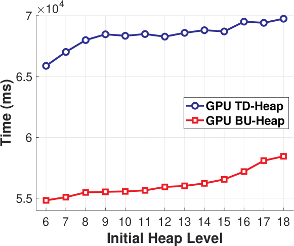
Figure 18. Performance w.r.t Initial Heap Size

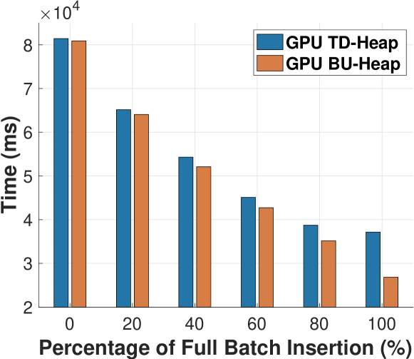
Figure 19. Performance w.r.t Partial Buffer

5.6. Impact of Partial Buffer and Partial Batch Insertion

We evaluate how partial batch updates influence the heap performance. We test the performance by inserting 512M items into an empty heap. We control the percentage of full batch insertions and let rest insertions be randomly generated partial batches. The results are shown in Fig. 19. As we can see, with the increase in the percentage of full batch insertions, the performance of becomes better. This is potentially because more threads are needed to insert the same number of keys, and it also cause more contention on the lock that protects the root node since inserting a partial batch will always require to lock the root node in both BU-INS/TD-DEL heap and TD-INS/TD-DEL heap. The implication is that, although partial batch is supported in the heap implementation, it would be good to avoid using partial batch insertions in real workloads if the total number of inserted keys is the same, since the overall performance difference could be up to 4X.

5.7. Concurrent Heap with Real World Applications

We apply our concurrent generalized heap to two real world applications: the single source shortest path (SSSP) algorithm and the 0/1 knapsack problem. Both applications can take the advantage of our concurrent heap by processing items with higher priority first. The purpose of this section is to shed light on the potential of incorporating our concurrent heap with many-core accelerators to solve real world applications. Further optimization to our concurrent heap with application-based asynchronous updates for insertion and deletion is possible, but we will leave it as our future work.

5.7.1. SSSP with Concurrent Heap

Gunrock(Wang et al., 2016) is a well known parallel iterative graph processing library on the GPU. It applies a compute-advance model to solve for applications like the SSSP such that at each iteration, nodes are classified as active nodes and inactive nodes by checking if their new distance bring an update to existing distance, after which only active nodes would be explored in the next iteration since inactive nodes will not bring updates to the final result.

Our implementation of the parallel SSSP algorithm is similar to Gunrock’s. At each iteration, we use our heap to store those active nodes with their current distance as the key. In this way, those nodes with the shortest distance would be explored first in the next iteration. As a result, our implementation tends to reduce the overhead of unnecessary updates and the number of active nodes being explored.

We use gunrock(Wang et al., 2016) as the baseline for comparison and we set a threshold $N$ such that only when the number of active nodes is larger than $N$, will we incorporate the algorithm with our concurrent heap. We use N=10K in our experiments. We choose 14 different real world graphs and describe the properties of these graphs in Table 2.

Table 2. Graph Information

Graph Name	# Nodes	# Edges	Type of Graph
AS365	3,799,275	22,736,152	2D FE triangular meshes
bundle_adj	513,351	20,721,402	Bundle adjustment problem
coPapersDBLP	540,486	30,491,458	DIMACS10 set
delaunay_n22	4,194,304	25,165,738	DIMACS10 set
hollywood-2009	1,139,905	115,031,232	Graph of movie actors
Hook_1498	1,498,023	62,415,468	3D mechanical problem
kron_g500_logn20	1,048,576	89,240,544	DIMACS10 set
Stanford_Berkeley	685,230	7,600,595	Berkeley-Stanford web graph
Long_Coup_dt0	1,470,152	88,559,144	Coupled consolidation problem
M6	3,501,776	21,003,872	2D FE triangular meshes
NLR	4,163,763	24,975,952	2D FE triangular meshes
rgg_n_2_20_s0	1,048,576	13,783,240	Undirected Random Graph
Serena	1,391,349	65,923,050	Structural Problem

Table 3. Parallel Single Source Shortest Path Performance

	Baseline		Heap Based SSSP w/ N=10K
Graphs	Computate	# Nodes	Heap	Compute	Total	# Nodes	Speedup
	Time(ms)	Visited	Time(ms)	Time(ms)	Time(ms)	Visited
AS365	654.44	19,664,769	193.43	422.12	615.55	11,843,368	1.06
bundle_adj	144.54	903,097	11	126.48	137.48	877,675	1.05
coPapersDBLP	46.13	981,876	12.52	25.46	37.98	710,794	1.21
delaunay_n22	1125.93	29,832,633	283.04	647.61	930.65	18,607,590	1.21
hollywood-2009	100.17	2,007,447	14.22	74.35	88.58	1,370,459	1.13
Hook_1498	233.76	2,786,271	31.39	182.52	213.91	1,756,776	1.09
kron_g500_logn20	117.79	2,590,570	28.72	73.1	101.82	860,552	1.16
Long_Coup_dt0	190.06	2,699,927	43.46	116.77	160.23	1,571,565	1.19
Stanford_Berkeley	55.3	530,294	5.17	52.54	57.71	462,860	0.96
M6	677.95	20,972,903	161.88	472.67	634.56	16,126,697	1.07
NLR	894.71	29,583,224	318.35	439.61	757.96	16,123,803	1.18
rgg_n_2_20_s0	920.27	7,112,685	46.44	701.78	748.22	5,871,411	1.23
Serena	124.16	2,594,858	27.98	84.94	112.93	1,498,836	1.1

We show the result of parallel SSSP in Table 3. For all the graphs we tested, we have an average of 1.13X overall speedup with the threshold $N$ = 10K compared to the baseline. The heap based sssp does not perform well on graph Stanford_Berkeley since it is a small graph, which means that the number of active nodes at each level is not large enough for the improvement brought by the heap to cover the overhead of it’s own operations.

In Table 3, we also list the time in milliseconds for sssp computation and heap operations separately. The computation time is the SSSP computation time, which includes processing times for node expanding, edge filtering and distance updating. The heap time is the time spent on the heap operations. The number of nodes visited represents the total number of times that nodes being explored during SSSP computation. With incorporation of our heap, the number of node visits is reduced remarkably compared to the baseline, which directly leads to the reduced sssp computation time.

5.7.2. 0/1 Knapsack with Concurrent Heap

The knapsack problem appears in real-world decision-making processes in a wide variety of fields. It defines as follows: given weights and benefits for some items and a knapsack with a limited capacity W, determine the maximum total benefit can be obtained in the knapsack. The 0/1 knapsack problem is a branch of the knapsack problem where one must either put the complete item in the knapsack or don’t pick it at all.

Branch and bound is an algorithm design paradigm, which is usually used for solving combinatorial optimization problems such as the 0/1 knapsack problem. The solution to the 0/1 knapsack problem can be expressed as a path in a binary decision tree where each level in the tree represents we either pick or do not pick an item. Thus, with n items, there are $2^{n}$ possible solutions. Instead of blindly checking for every possible solution for the maximum benefit under certain capacity, we can prune the search space by comparing the bound (the best possible benefit we could gain if we choose this node) of a node with the current maximum benefit to see if it is worth continue exploring.

A simple sequential implementation of such algorithm is to enqueue to-explore nodes into a priority queue with their current benefits as the key values and always choose to explore nodes with largest benefit first. On one hand, it is a greedy approach that would give optimal solution despite that it might encounter several local optimal before get to the global optima. On the other hand, if nodes with larger benefit are explored first, we can skip exploring certain nodes with a bound that is smaller than the max current benefit. We implement a parallel GPU knapsack algorithm based on the sequential version with our concurrent heap to show that the incorporation of our concurrent heap accelerates knapsack computation.

Since parallelizing node exploration might result in unnecessary growth in heap size, we also apply a technique which filters invalid nodes when heap size is larger than a certain threshold before the algorithm continues to explore more nodes. We name this version as knapsack with garbage collection (GC).

Table 4. Datasets for 0/1 Knapsack Problem

Dataset	Type	Size	Range
ks_sc_700_18k	Strongly Correlated	700	18000
ks_sc_800_18k	Strongly Correlated	800	18000
ks_sc_200_7k	Strongly Correlated	200	7000
ks_asc_750_16k	Almost Strongly Correlated	750	16000
ks_asc_1300_6k	Almost Strongly Correlated	1300	6000
ks_asc_500_7k	Almost Strongly Correlated	500	7000
ks_esc_900_18k	Even-odd Strongly Correlated	900	18000
ks_esc_1200_13k	Even-odd Strongly Correlated	1200	13000
ks_esc_400_8k	Even-odd Strongly Correlated	400	8000
ks_ss_100_18k	Subset Sum	100	18000
ks_ss_1250_12k	Subset Sum	1250	12000
ks_ss_1300_14k	Subset Sum	1300	14000

Table 5. 0/1 Knapsack Problem with heap

	CPU w/		GPU w/ concurrent			GPU w/ concurrent
	Priority Queue		heap			heap and GC.
Dataset	Time	# Nodes	Time	# Nodes	SpeedUp	Time	# Nodes	SpeedUp
	(ms)	Explored	(ms)	Explored		(ms)	Explored
ks_sc_700_18k	825.70	782802	670.57	813089	1.23	595.58	810717	1.39
ks_sc_800_18k	977.49	923255	757.06	955374	1.29	708.02	956514	1.38
ks_sc_200_7k	202.40	243106	199.76	249373	1.01	205.27	249935	0.99
ks_asc_750_16k	757.17	709267	722.90	389249	1.05	566.17	445231	1.34
ks_asc_1300_6k	5239.97	4934552	5118.03	2832737	1.02	4115.55	2404241	1.27
ks_asc_500_7k	502.37	475402	549.10	296824	0.91	499.03	295951	1.01
ks_esc_900_18k	1128.4	1080182	848.65	1123920	1.33	796.58	1124880	1.42
ks_esc_1200_13k	2013.06	1950260	2066.64	2002002	0.97	1357.75	1770747	1.48
ks_esc_400_8k	355.25	399185	346.53	418925	1.03	348.52	421504	1.02
ks_ss_100_18k	42.38	54278	3.55	55	3.48	11.92	55	12.19
ks_ss_1250_12k	20.27	23886	4.30	94	4.12	4.72	94	4.92
ks_ss_1300_14k	25.02	25305	19.64	9452	1.27	18.01	8528	1.39

In (Martello et al., 1999), S. Martello et al. defined and tested with several types of instances of knapsack problems. Using the same data generation tool, we generated 12 knapsack datasets to demonstrate the potential of our concurrent heap. We describe the properties of these datasets in Table 4.

We compared the running time in milliseconds and the number of explored nodes between sequential and GPU knapsack in Table 5. For all the datasets we tested we obtain an average overall speedup of 2.31X for GPU knapsack and 2.48X for GPU knapsack with garbage collection.

We find that our GPU knapsack algorithms with concurrent heap performs particularly well with Subset-sum(ss) instances, with a maximum speedup up to 12.19X compared to sequential version. Also, the number of nodes explored for GPU knapsack is significantly smaller than that of sequential knapsack. Because of the greedy property of the branch and bound algorithm, it does not guarantee the path its exploring will lead to a global optimal solution, it is possible, especially with the Subset-sum instances where the benefit of an item is equal to the weight of it. On the other hand, parallelizing the branch and bound algorithm with our concurrent heap allows it to solve for a large amount of potential solutions that are prioritized by their current benefit simultaneously, which can lead to a faster convergence of the global optimal solution.

Theoretically, parallelizing node exploration in branch and bound knapsack problem may cause an exponential growth in the queue size since it performs parallel explorations for nodes in a binary decision tree. However, according to our experiments, we find that the GPU knapsack sometimes results in less node exploration because while nodes with higher benefit are explored earlier than other nodes, there are chances where the current max benefit converges fast enough so that the nodes with lower priority quickly become invalid for exploration since it’s bound become smaller than the max benefit, which leads to a reduction in exploring time and correspondingly an increase of overall performance.

6. Related Work

CPU Parallel Heap Algorithms The most popular CPU approach (Nageshwara and Kumar, 1988; Ayani, 1990; Hunt et al., 1996; Shavit and Zemach, 1999; Prasad and Sawant, 1995) to gain parallelism for parallel heap is by supporting concurrent insert or/and delete operations. Rao and Kumar(Nageshwara and Kumar, 1988) proposed a scheme that used multiple mutual exclusion locks to protect each node in the heap. They also proceeded insertions in the top-down manner to avoid deadlock while insertions for the conventional heap follow a bottom-up manner. Rassul(Ayani, 1990) proposed LR-algorithm which was an extension to Rao and Kumar’s method that scatter the accesses of different operations to reduce the contention. Hunt and others(Hunt et al., 1996) present a lock-based heap algorithm that supports insertion and deletion in an opposite directions. Deo and Prasad(Deo and Prasad, 1992) increased the node capacity. However, their algorithm does not support concurrent insertions/deletions.

All these parallel heap algorithms on CPUs cannot be applied to GPUs directly because of the unique SIMT execution model employed by moder GPUs. For parallel algorithms on GPUs, the optimization for thread divergence, memory coalescing and synchronization need to be taken into account.

GPU Parallel Heap Algorithms Parallel Heap algorithms are less studied on GPUs. He (He et al., 2012) introduced a parallel heap algorithms for many-fore architectures like GPUs. Their algorithm exploited the parallelism of the parallel heap by increasing the node capacity, like the idea in (Deo and Prasad, 1992), and pipelining the insert and delete operations. However, their approach did not exploit the parallelism for concurrent operations at the same level of the heap. Also they need a global barrier to synchronize all threads after the insert or delete updates at every levels which brought extra heavy overhead.

7. Conclusion

This work proposes a concurrent heap implementation that is friendly to many-core accelerators. We develop a generalized heap and support both intra-node and inter-node parallelism. We also prove that our two heap implementations are linearizable. We evaluate our concurrent heap thoroughly and show a maximum 19.49X speedup compared to the sequential CPU implementation and 2.11X speedup compared with the existing GPU implementation (He et al., 2012).

- (1)
- Ayani (1990) R. Ayani. 1990. LR-algorithm: concurrent operations on priority queues. In Proceedings of the Second IEEE Symposium on Parallel and Distributed Processing 1990. IEEE, Piscataway, NJ, USA, 22–25. https://doi.org/10.1109/SPDP.1990.143500
- Corporation (2010) NVIDIA Corporation. 2010. NVIDIA’s Next Generation CUDA Compute Architecture: Kepler GK110: The Fastest, Most Efficient HPC Architecture Ever Built. https://www.nvidia.com/content/PDF/kepler/NVIDIA-Kepler-GK110-Architecture-Whitepaper.pdf
- Deo and Prasad (1992) Narsingh Deo and Sushil Prasad. 1992. Parallel heap: An optimal parallel priority queue. The Journal of Supercomputing 6, 1 (1992), 87–98.
- Green et al. (2012) Oded Green, Robert McColl, and David A Bader. 2012. GPU merge path: a GPU merging algorithm. In Proceedings of the 26th ACM international conference on Supercomputing. ACM, ACM, New York, NY, USA, 331–340.
- He et al. (2012) X. He, D. Agarwal, and S. K. Prasad. 2012. Design and implementation of a parallel priority queue on many-core architectures. In 2012 19th International Conference on High Performance Computing. IEEE, Piscataway, NJ, USA, 1–10. https://doi.org/10.1109/HiPC.2012.6507490
- Herlihy and Wing (1990) Maurice P Herlihy and Jeannette M Wing. 1990. Linearizability: A correctness condition for concurrent objects. ACM Transactions on Programming Languages and Systems (TOPLAS) 12, 3 (1990), 463–492.
- Hunt et al. (1996) Galen C Hunt, Maged M Michael, Srinivasan Parthasarathy, and Michael L Scott. 1996. An efficient algorithm for concurrent priority queue heaps. Inform. Process. Lett. 60, 3 (1996), 151–157.
- Kumar et al. (2008) S. Kumar, D. Kim, M. Smelyanskiy, Y. Chen, J. Chhugani, C. J. Hughes, C. Kim, V. W. Lee, and A. D. Nguyen. 2008. Atomic Vector Operations on Chip Multiprocessors. In 2008 International Symposium on Computer Architecture. IEEE, Piscataway, NJ, USA, 441–452. https://doi.org/10.1109/ISCA.2008.38
- Martello et al. (1999) Silvano Martello, David Pisinger, and Paolo Toth. 1999. Dynamic programming and strong bounds for the 0-1 knapsack problem. Management Science 45, 3 (1999), 414–424.
- Moscovici et al. (2017) N. Moscovici, N. Cohen, and E. Petrank. 2017. A GPU-Friendly Skiplist Algorithm. In 2017 26th International Conference on Parallel Architectures and Compilation Techniques (PACT). IEEE, Piscataway, NJ, USA, 246–259. https://doi.org/10.1109/PACT.2017.13
- Nageshwara and Kumar (1988) RV Nageshwara and Vipin Kumar. 1988. Concurrent access of priority queues. IEEE Trans. Comput. 37, 12 (1988), 1657–1665.
- Prasad and Sawant (1995) Sushil K Prasad and Sagar I Sawant. 1995. Parallel heap: A practical priority queue for fine-to-medium-grained applications on small multiprocessors. In Parallel and Distributed Processing, 1995. Proceedings. Seventh IEEE Symposium on. IEEE, IEEE, Piscataway, NJ, USA, 328–335.
- Shavit and Taubenfeld (2016) Nir Shavit and Gadi Taubenfeld. 2016. The computability of relaxed data structures: queues and stacks as examples. Distributed Computing 29, 5 (2016), 395–407.
- Shavit and Zemach (1999) Nir Shavit and Asaph Zemach. 1999. Scalable concurrent priority queue algorithms. In Proceedings of the eighteenth annual ACM symposium on Principles of distributed computing. ACM, ACM, New York, NY, USA, 113–122.
- Wang et al. (2016) Yangzihao Wang, Andrew Davidson, Yuechao Pan, Yuduo Wu, Andy Riffel, and John D. Owens. 2016. Gunrock: A High-performance Graph Processing Library on the GPU, In PPOPP. SIGPLAN Not. 51, 8, Article 11, 12 pages. https://doi.org/10.1145/3016078.2851145
- Wong et al. (2010) Henry Wong, Misel-Myrto Papadopoulou, Maryam Sadooghi-Alvandi, and Andreas Moshovos. 2010. Demystifying GPU microarchitecture through microbenchmarking. In 2010 IEEE International Symposium on Performance Analysis of Systems & Software (ISPASS). IEEE, Piscataway, NJ, USA, 235–246.
- Zhang et al. (2011) Eddy Z. Zhang, Yunlian Jiang, Ziyu Guo, Kai Tian, and Xipeng Shen. 2011. On-the-fly Elimination of Dynamic Irregularities for GPU Computing. SIGPLAN Not. 46, 3 (March 2011), 369–380. https://doi.org/10.1145/1961296.1950408