Global optimization via inverse distance weighting
and radial basis functions

Abstract

Global optimization problems whose objective function is expensive to evaluate can be solved effectively by recursively fitting a surrogate function to function samples and minimizing an acquisition function to generate new samples. The acquisition step trades off between seeking for a new optimization vector where the surrogate is minimum (exploitation of the surrogate) and looking for regions of the feasible space that have not yet been visited and that may potentially contain better values of the objective function (exploration of the feasible space). This paper proposes a new global optimization algorithm that uses a combination of inverse distance weighting (IDW) and radial basis functions (RBF) to construct the acquisition function. Rather arbitrary constraints that are simple to evaluate can be easily taken into account. Compared to Bayesian optimization, the proposed algorithm, that we call GLIS (GLobal minimum using Inverse distance weighting and Surrogate radial basis functions), is competitive and computationally lighter, as we show in a set of benchmark global optimization and hyperparameter tuning problems. MATLAB and Python implementations of GLIS are available at http://cse.lab.imtlucca.it/~bemporad/glis.

Keywords: Global optimization, inverse distance weighting, Bayesian optimization, radial basis functions, surrogate models, derivative-free algorithms, black-box optimization.

1 Introduction

Many problems in machine learning and statistics, engineering design, physics, medicine, management science, and in many other fields, require finding a global minimum of a function without derivative information; see, e.g., the excellent survey on derivative-free optimization [32]. Some of the most successful approaches for derivative-free global optimization include deterministic methods based on recursively splitting the feasible space in rectangles, such as the DIRECT (DIvide a hyper-RECTangle) [22] and Multilevel Coordinate Search (MCS) [18] algorithms, and stochastic methods such as Particle Swarm Optimization (PSO) [12], genetic algorithms [43], and evolutionary algorithms [16].

The aforementioned methods can be very successful in reaching a global minimum without any assumption on convexity and smoothness of the function, but may result in evaluating the function a large number of times during the execution of the algorithm. In many problems, however, the objective function is a black box that can be very time-consuming to evaluate. For example, in hyperparameter tuning of machine learning algorithms, one needs to run a large set of training tests per hyperparameter choice; in structural engineering design, testing the resulting mechanical property corresponding to a given choice of parameters may involve several hours for computing solutions to partial differential equations; in control systems design, testing a combination of controller parameters involves running a real closed-loop experiment, which is time consuming and costly. For this reason, many researchers have been studying algorithms for black-box global optimization that aim at minimizing the number of function evaluations by replacing the function to minimize with a surrogate function [21]. The latter is obtained by sampling the objective function and interpolating the samples with a map that, compared to the original function, is very cheap to evaluate. The surrogate is then used to solve a (much cheaper) global optimization problem that decides the new point the original function must be evaluated. A better-quality surrogate is then created by also exploiting the new sample and the procedure is iterated. For example, quadratic surrogate functions are used in the well known global optimization method NEWUOA [30].

As underlined by several authors (see, e.g., [21]), purely minimizing the surrogate function may lead to converge to a point that is not the global minimum of the black-box function. To take into account the fact that the surrogate and the true objective function differ from each other in an unknown way, the surrogate is typically augmented by an extra term that takes into account such an uncertainty. The resulting acquisition function is therefore minimized instead for generating a new sample of the optimization vector, trading off between seeking for a new vector where the surrogate is small and looking for regions of the feasible space that have not yet been visited.

Bayesian Optimization (BO) is a popular class of global optimization methods based on surrogates that, by modeling the black box function as a Gaussian process, enables one to quantify in statistical terms the discrepancy between the two functions, an information that is taken into account to drive the search. BO has been studied since the sixties in global optimization [25] and in geostatistics [26] under the name of Kriging methods; it become popular to solve problems of Design and Analysis of Computer Experiments (DACE) [34], see for instance the popular Efficient Global Optimization (EGO) algorithm [23]. It is nowadays very popular in machine learning for tuning hyperparameters of different algorithms [9, 37, 35, 13].

Motivated by learning control systems from data [29] and self-calibration of optimal control parameters [14], in this paper we propose an alternative approach to solve global optimization problems in which the objective function is expensive to evaluate that is based on Inverse Distance Weighting (IDW) interpolation [36, 24] and Radial Basis Functions (RBFs) [17, 27]. The use of RBFs for solving global optimization problems was already adopted in [15, 11], in which the acquisition function is constructed by introducing a “measure of bumpiness”. The author of [15] shows that such a measure has a relation with the probability of hitting a lower value than a given threshold of the underlying function, as used in Bayesian optimization. RBFs were also adopted in [31], with additional constraints imposed to make sure that the feasible set is adequately explored. In this paper we use a different acquisition function based on two components: an estimate of the confidence interval associated with RBF interpolation as suggested in [24], and a new measure based on inverse distance weighting that is totally independent of the underlying black-box function and its surrogate. Both terms aim at exploring the domain of the optimization vector. Moreover, arbitrary constraints that are simple to evaluate are also taken into account, as they can be easily imposed during the minimization of the acquisition function.

Compared to Bayesian optimization, our non-probabilistic approach to global optimization is very competitive, as we show in a set of benchmark global optimization problems and on hyperparameter selection problems, and also computationally lighter than off-the-shelf implementations of BO.

A preliminary version of this manuscript was made available in [4] and later extended in [5] to solve preference-based optimization problems. MATLAB and a Python implementations of the proposed approach and of the one of [5] are available for download at http://cse.lab.imtlucca.it/~bemporad/glis. For an application of the GLIS algorithm proposed in this paper to learning optimal calibration parameters in embedded model predictive control applications the reader is referred to [14].

The paper is organized as follows. After stating the global optimization problem we want to solve in Section 2, Sections 3 and 4 deal with the construction of the surrogate and acquisition functions, respectively. The proposed global optimization algorithm is detailed in Section 5 and several results are reported in Section 6. Finally, some conclusions are drawn in Section 7.

2 Problem formulation

Consider the following constrained global optimization problem

$$\begin{array}[]{rl}\min_{x}&f(x)\\ \mathop{\rm s.t.}\nolimits&\ell\leq x\leq u\\ &x\in\mathcal{X}\end{array}$$ (1)

where $f:{\mathbb{R}}^{n}\to{\mathbb{R}}$ is an arbitrary function of the optimization vector $x\in{\mathbb{R}}^{n}$, $\ell,u\in{\mathbb{R}}^{n}$ are vectors of lower and upper bounds, and $\mathcal{X}\subseteq{\mathbb{R}}^{n}$ imposes further arbitrary constraints on $x$. Typically $\mathcal{X}=\{x\in{\mathbb{R}}^{n}:\ g(x)\leq 0\}$, where the vector function $g:{\mathbb{R}}^{n}\to{\mathbb{R}}^{q}$ defines inequality constraints, with $q=0$ meaning that no inequality constraint is enforced; for example, linear inequality constraints are defined by setting $g(x)=Ax-b$, with $A\in{\mathbb{R}}^{q\times n}$, $b\in{\mathbb{R}}^{q}$, $q\geq 0$. We are particularly interested in problems as in (1) such that $f(x)$ is expensive to evaluate and its gradient is not available, while the condition $x\in\mathcal{X}$ is easy to evaluate. Although not comprehensively addressed in this paper, we will show that our approach also tolerates noisy evaluations of $f$, that is if we measure $y=f(x)+\varepsilon$ instead of $f(x)$, where $\varepsilon$ is an unknown quantity. We will not make any assumption on $f$, $g$, and $\varepsilon$. In (1) we do not include possible linear equality constraints $A_{e}x=b_{e}$, as they can be first eliminated by reducing the number of optimization variables.

3 Surrogate function

Assume that we have collected a vector $F=[f_{1}\ \ldots\ f_{N}]^{\prime}$ of $N$ samples $f_{i}=f(x_{i})$ of $f$, $F\in{\mathbb{R}}^{N}$ at corresponding points $X=[x_{1}\ \ldots\ x_{N}]^{\prime}$, $X\in{\mathbb{R}}^{N\times n}$, with $x_{i}\neq x_{j}$, $\forall i\neq j$, $i,j=1,\ldots,N$. We consider next two types of surrogate functions, namely Inverse Distance Weighting (IDW) functions [36, 24] and Radial Basis Functions (RBFs) [15, 27].

3.1 Inverse distance weighting functions

Given a generic new point $x\in{\mathbb{R}}^{n}$ consider the vector function of squared Euclidean distances $d^{2}:{\mathbb{R}}^{n\times n}\to{\mathbb{R}}^{N}$

$$d^{2}(x,x_{i})=(x_{i}-x)^{\prime}(x_{i}-x),\ i=1,\ldots,N$$ (2)

In standard IDW functions [36] the weight functions $w_{i}:{\mathbb{R}}^{n}\setminus\{x_{i}\}\to{\mathbb{R}}$ are defined by the inverse squared distances

$$w_{i}(x)=\frac{1}{d^{2}(x,x_{i})}$$ (3a)

The alternative weighting function

$$w_{i}(x)=\frac{e^{-d^{2}(x,x_{i})}}{d^{2}(x,x_{i})}$$ (3b)

suggested in [24] has the advantage of being similar to the inverse squared distance in (3a) for small values of $d^{2}$, but makes the effect of points $x_{i}$ located far from $x$ fade out quickly due to the exponential term.

By defining for $i=1,\ldots,N$ the following functions $v_{i}:{\mathbb{R}}^{n}\to{\mathbb{R}}$ as

$$v_{i}(x)=\left\{\begin{array}[]{ll}1&\mbox{if}\ x=x_{i}\\ 0&\mbox{if}\ x=x_{j},\ j\neq i\\ \displaystyle{\frac{w_{i}(x)}{\sum_{j=1}^{N}w_{j}(x)}}&\mbox{otherwise}\end{array}\right.$$ (4)

the surrogate function $\hat{f}:{\mathbb{R}}^{n}\to{\mathbb{R}}$

$$\hat{f}(x)=\sum_{i=1}^{N}v_{i}(x)f_{i}$$ (5)

is an IDW interpolation of $(X,F)$.

Lemma 1

The IDW interpolation function $\hat{f}$ defined in (5) enjoys the following properties:

1. $\hat{f}(x_{j})=f_{j}$, $\forall j=1,\ldots,N$;

2. $\min_{j}\{f_{j}\}\leq\hat{f}(x)\leq\max_{j}\{f_{j}\}$, $\forall x\in{\mathbb{R}}^{n}$;

3. $\hat{f}$ is differentiable everywhere on ${\mathbb{R}}^{n}$ and in particular $\nabla f(x_{j})=0$ for all $j=1,\ldots,N$.

The proof of Lemma 1 is very simple and is reported in Appendix A.

Note that in [24] the authors suggest to improve the surrogate function by adding a regression model in (5) to take global trends into account. In our numerical experiments we found, however, that adding such a term does not lead to significant improvements of the proposed global optimization algorithm.

A one-dimensional example of the IDW surrogate $\hat{f}$ sampled at five different points of the scalar function

$$f(x)=\left(1+\frac{x\sin(2x)\cos(3x)}{1+x^{2}}\right)^{2}+\frac{x^{2}}{12}+\frac{x}{10}$$ (6)

is depicted in Figure 1. The global optimizer is $x^{*}\approx-0.9599$ corresponding to the global minimum $f(x^{*})\approx 0.2795$.

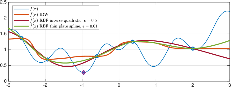
Figure 1: A scalar example of $f(x)$ as in (6) (blue) sampled at $N=5$ points (blue circles), IDW surrogate $\hat{f}(x)$ (orange) with $w_{i}(x)$ as in (3b), RBF inverse quadratic with $\epsilon=0.5$ (red), RBF thin plate spline surrogate with $\epsilon=0.01$ (green), global minimum (purple diamond)

3.2 Radial basis functions

A possible drawback of the IDW function $\hat{f}$ defined in (5) is due to property P3: As the number $N$ of samples increases, the surrogate function tends to ripple, having its derivative to always assume zero value at samples. An alternative is to use a radial basis function (RBF) [15, 27] as a surrogate function. These are defined by setting

$$\hat{f}(x)=\sum_{i=1}^{N}\beta_{i}\phi(\epsilon d(x,x_{i}))$$ (7)

where $d:{\mathbb{R}}^{n\times n}\to{\mathbb{R}}$ is the function defining the Euclidean distance as in (2), $d(x,x_{i})=\|x-x_{i}\|_{2}$, $\epsilon>0$ is a scalar parameter, $\beta_{i}$ are coefficients to be determined as explained below, and $\phi:{\mathbb{R}}\to{\mathbb{R}}$ is a RBF. Popular examples of RBFs are

$$\begin{array}[]{llll}\phi(\epsilon d)=\frac{1}{1+(\epsilon d)^{2}}&\mbox{\small(inverse quadratic)}&\phi(\epsilon d)=e^{-(\epsilon d)^{2}}&\mbox{\small(Gaussian)}\\[10.00002pt] \phi(\epsilon d)=\sqrt{1+(\epsilon d)^{2}}&\mbox{\small(multiquadric)}&\phi(\epsilon d)=(\epsilon d)^{2}\log(\epsilon d)&\mbox{\small(thin plate spline)}\\[10.00002pt] \phi(\epsilon d)=\epsilon d&\mbox{\small(linear)}&\phi(\epsilon d)=\frac{1}{\sqrt{1+(\epsilon d)^{2}}}&\mbox{\small(inverse multiquadric)}\end{array}$$ (8)

The coefficient vector $\beta=[\beta_{1}\ \ldots\ \beta_{N}]^{\prime}$ is obtained by imposing the interpolation condition

$$\hat{f}(x_{i})=f_{i},\ i=1,\ldots,N$$ (9)

Condition (9) leads to solving the linear system

$$M\beta=F$$ (10a)

where $$M N\times N (i,j)$$ is the symmetric matrix whose -entry is

$$M_{ij}=\phi(\epsilon d(x_{i},x_{j}))$$ (10b)

with $$M_{ii}=1 M_{ii}=\lim_{d\rightarrow 0}\phi(\epsilon d)=0 f x_{N+1} M \phi(\epsilon d(x_{N+1},x_{j})) j=1,\ldots,N+1$$ for all the RBF type listed in (8) but the linear and thin plate spline, for which . Note that if function is evaluated at a new sample , matrix only requires adding the last row/column obtained by computing for all .

As highlighted in [15, 21], matrix $M$ might be singular, even if $x_{i}\neq x_{j}$ for all $i\neq j$. To prevent issues due to a singular $M$, [15, 21] suggest using a surrogate function given by the sum of a RBF and a polynomial function of a certain degree. To also take into account unavoidable numerical issues when distances between sampled points get close to zero, which will easily happen as new samples are added towards finding a global minimum, in this paper we suggest instead to use a singular value decomposition (SVD) $M=U\Sigma V^{\prime}$ of $M$ . By neglecting singular values below a certain positive threshold $\epsilon_{\rm SVD}$, we can approximate $\Sigma=\left[\begin{smallmatrix}\Sigma_{1}&0\\ 0&0\end{smallmatrix}\right]$, where $\Sigma_{1}$ collects all singular values $\sigma_{i}\geq\epsilon_{\rm SVD}$, and accordingly split $V=[V_{1}\ V_{2}]$, $U=[U_{1}\ U_{2}]$ so that

$$\beta=V_{1}\Sigma_{1}^{-1}U_{1}^{\prime}F$$ (10c)

The threshold $\epsilon_{\rm SVD}$ turns out to be useful when dealing with noisy measurements $y=f(x)+\varepsilon$ of $f$. Figure 2 shows the approximation $\hat{f}$ obtained from 50 samples with $\varepsilon$ normally distributed around zero with standard deviation $0.1$, when $\epsilon_{\rm SVD}=10^{-2}$.

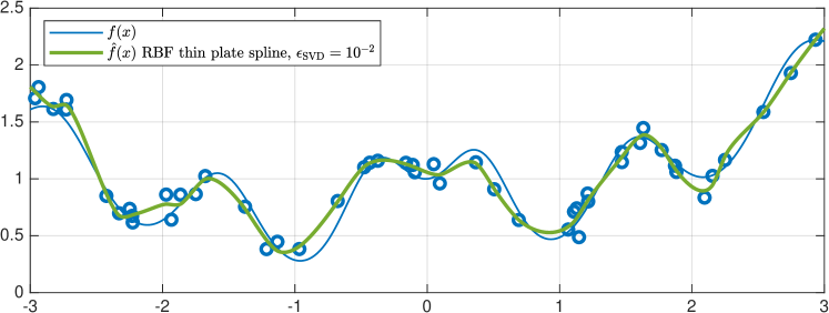
Figure 2: Function $f(x)$ as in (6) is sampled 50 times, with each sample corrupted by noise $\varepsilon\sim{\mathcal{N}}(0,10^{-2})$ (blue). The RBF thin plate spline surrogate with $\epsilon=0.01$ (green) is obtained by setting $\epsilon_{\rm SVD}=10^{-2}$

A drawback of RBFs, compared to IDW functions, is that property P2 is no longer satisfied, with the consequence that the surrogate may extrapolate large values $\hat{f}(x)$ where $f(x)$ is actually small, and vice versa. See the examples plotted in Figure 1. On the other hand, while differentiable everywhere, RBFs do not necessarily have zero gradients at sample points as in P3, which is favorable to better approximate the underlying function with limited samples. For the above reasons, we will mostly focus on RBF surrogates in our numerical experiments.

3.3 Scaling

To take into account that different components $x^{j}$ of $x$ may have different ranges $u^{j}-\ell^{j}$, we simply rescale the variables in optimization problem (1) so that they all range in $[-1,1]$. To this end, we first possibly tighten the given box constraints $B_{\ell,u}=\{x\in{\mathbb{R}}^{n}:\ell\leq x\leq u\}$ by computing the bounding box $B_{\ell_{s},u_{s}}$ of the set $\{x\in{\mathbb{R}}^{n}:\ x\in\mathcal{X}\}$ and replacing $B_{\ell,u}\leftarrow B_{\ell,u}\cap B_{\ell_{s},u_{s}}$. The bounding box $B_{\ell_{s},u_{g}}$ is obtained by solving the following $2n$ optimization problems

$$\begin{array}[]{rcl}\ell_{g}^{i}&=&\min_{x\in\mathcal{X}}e_{i}^{\prime}x\\ u_{g}^{i}&=&\max_{x\in\mathcal{X}}e_{i}^{\prime}x\end{array}$$ (11a)

where $$e_{i} i i=1,\ldots,n \mathcal{X}=\{x\in{\mathbb{R}}^{n}\ Ax\leq b\} \ell,u$$ is the th column of the identity matrix, . In case of linear inequality constraints , the problems in (11a) can be solved by linear programming (LP), see (17) below. Since now on, we assume that are replaced by

$$\begin{array}[]{rcl}\ell&\leftarrow&\max\{\ell,\ell_{g}\}\\ u&\leftarrow&\min\{u,u_{g}\}\end{array}$$ (11b)

where “$\min$ ”and “$\max$” in (11b) operate component-wise. Next, we introduce scaled variables $\bar{x}\in{\mathbb{R}}^{n}$ whose relation with $x$ is

$$x^{j}(\bar{x})=\bar{x}^{j}(u^{j}-\ell^{j})+\frac{u^{j}+\ell^{j}}{2}$$ (12a)

for all $$j=1,\ldots,n$$ and finally formulate the following scaled global optimization problem

$$\begin{array}[]{rl}\min&f_{s}(\bar{x})\\ \mathop{\rm s.t.}\nolimits&-1\leq\bar{x}^{j}\leq 1,\ j=1,\ldots,n\\ &x\in\mathcal{X}_{s}\end{array}$$ (12b)

where $$f_{s}:{\mathbb{R}}^{n}\to{\mathbb{R}} \mathcal{X}_{s}$$, are defined as

$$\begin{array}[]{rcl}f_{s}(\bar{x})&=&f(x(\bar{x}))\\ \mathcal{X}_{s}&=&\{\bar{x}\in{\mathbb{R}}^{n}:\ x(\bar{x})\in\mathcal{X}\}\end{array}$$

In case $$\mathcal{X}$$ is a polyhedron we have

$$\mathcal{X}_{s}=\{\bar{x}:\ \bar{A}\bar{x}\leq\bar{b}\}$$ (12c)

where $$\bar{A} \bar{b} A,b$$, are a rescaled version of defined as

$$\begin{array}[]{rcl}\bar{A}&=&A\mathop{\rm diag}\nolimits(u-\ell)\\ \bar{b}&=&b-A(\frac{u+\ell}{2})\end{array}$$ (12d)

and $\mathop{\rm diag}\nolimits(u-\ell)$ is the diagonal matrix whose diagonal elements are the components of $u-\ell$.

Note that, when approximating $f_{s}$ with $\hat{f}_{s}$, we use the squared Euclidean distances

$$d^{2}(\bar{x},\bar{x}_{i})=\sum_{h=1}^{n}(\bar{x}-\bar{x}_{i})^{2}=\sum_{h=1}^{n}\left(\theta_{h}(x^{h}-x^{h}_{i})\right)^{p_{h}}$$

where the scaling factors $\theta^{h}=u^{h}-\ell^{h}$ and $p_{h}\equiv 2$ are constant. Therefore, finding a surrogate $\hat{f}_{s}$ of $f_{s}$ in $[-1,1]$ is equivalent to finding a surrogate $\hat{f}$ of $f$ under scaled distances. This is a much simpler scaling approach than computing the scaling factors $\theta^{h}$ and power $p$ as it is common in stochastic process model approaches such as Kriging methods [34, 23]. As highlighted in [21], Kriging methods use radial basis functions $\phi(x_{i},x_{j})=e^{-\sum_{h=1}^{n}\theta_{h}|x_{i}^{h}-x_{j}^{h}|^{p_{h}}}$, a generalization of Gaussian RBF functions in which the scaling factors and powers that are recomputed as the data set $X$ changes.

Note also that the approach adopted in [5] for scaling automatically the surrogate function via cross-validation could be also used here, as well as other approaches specific for RBFs such as Rippa’s method [33]. In our numerical experiments we have found that adjusting the RBF parameter $\epsilon$ via cross-validation, while increasing the computational effort, does not provide significant benefit. What is in fact most critical is the tradeoff between exploitation of the surrogate and exploration of the feasible set, that we discuss in the next section.

4 Acquisition function

As mentioned earlier, minimizing the surrogate function to get a new sample $x_{N+1}$ $=$ $\arg\min\hat{f}(x)$ subject to $\ell\leq x\leq u$ and $x\in\mathcal{X}$, evaluating $f(x_{N+1})$, and iterating over $N$ may easily miss the global minimum of $f$. This is particularly evident when $\hat{f}$ is the IDW surrogate (5), that by Property P2 of Lemma 1 has a global minimum at one of the existing samples $x_{i}$. Besides exploiting the surrogate function $\hat{f}$, when looking for a new candidate optimizer $x_{N+1}$ it is therefore necessary to add to $\hat{f}$ a term for exploring areas of the feasible space that have not yet been probed.

In Bayesian optimization, such an exploration term is provided by the covariance associated with the Gaussian process. A function measuring “bumpiness” of a surrogate RBF function was used in [15]. Here instead we propose two functions that provide exploration capabilities, that can be used in alternative to each other or in a combined way. First, as suggested in [24] for IDW functions, we consider the confidence interval function $s:{\mathbb{R}}^{n}\to{\mathbb{R}}$ for $\hat{f}$ defined by

$$s(x)=\sqrt{\sum_{i=1}^{N}v_{i}(x)(f_{i}-\hat{f}(x))^{2}}$$ (13)

We will refer to function $s$ as the IDW variance function associated with $(X,F)$. Clearly, when $\hat{f}(x_{i})=f(x_{i})$ then $s(x_{i})=0$ for all $i=1,\ldots,N$ (no uncertainty at points $x_{i}$ where $f$ is evaluated exactly). See Figure 3 for a noise-free example and Figure 4 for the case of noisy measurements of $f$.

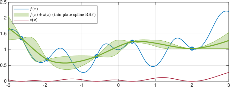
Figure 3: Plot of $\hat{f}(x)\pm s(x)$ and $z(x)$ for the scalar example as in Figure 1, with $w_{i}(x)$ as in (3a) and $f$ as in (6)

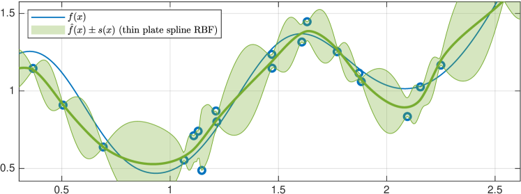
Figure 4: Zoomed plot of $\hat{f}(x)\pm s(x)$ for the scalar example as in Figure 3 when 50 samples of $f(x)$ are measured with noise $\varepsilon\sim{\mathcal{N}}(0,10^{-2})$ and $\epsilon_{\rm SVD}=10^{-2}$

Second, we introduce the new IDW distance function $z:{\mathbb{R}}^{n}\to{\mathbb{R}}$ defined by

$$z(x)=\left\{\begin{array}[]{ll}0&\mbox{if}\ x\in\{x_{1},\ldots,x_{N}\}\\ \frac{2}{\pi}\tan^{-1}\left(\frac{1}{\sum_{i=1}^{N}w_{i}(x)}\right)&\mbox{otherwise}\end{array}\right.$$ (14)

where $w_{i}(x)$ is given by either (3a) or (3b). The rationale behind (14) is that $z(x)$ is zero at sampled points and grows in between. The arc tangent function in (14) avoids that $z(x)$ grows excessively when $x$ is located far away from all sampled points. Figure 5 shows a scalar example of function $v_{1}$ and $z$.

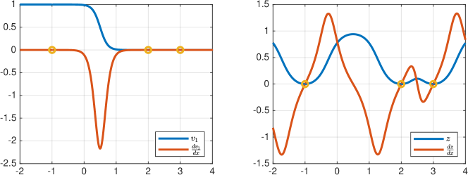
Figure 5: A scalar example of function $v_{1}(x)$ and $z(x)$ for $x_{j}=j$, $j=1,2,3$

Given parameters $\alpha,\delta\geq 0$ and $N$ samples $(X,F)$, we define the following acquisition function $a:{\mathbb{R}}^{n}\to{\mathbb{R}}$

$$a(x)=\hat{f}(x)-\alpha s(x)-\delta\Delta Fz(x)$$ (15)

where $\Delta F=\max\{\max_{i}\{f_{i}\}-\min_{i}\{f_{i}\},\epsilon_{\rm\Delta F}\}$ is the range of the observed samples $F$ and the threshold $\epsilon_{\rm\Delta F}>0$ is introduced to prevent the case in which $f$ is not a constant function but, by chance, all sampled values $f_{i}$ are equal. Scaling $z$ by $\Delta F$ ease the selection of the hyperparameter $\delta$, as the amplitude of $\Delta Fz$ is comparable to that of $\hat{f}$.

As we will detail next, given $N$ samples $(X,F)$ a global minimum of the acquisition function (15) is used to define the $(N+1)$-th sample $x_{N+1}$ by solving the global optimization problem

$$x_{N+1}=\arg\min_{\ell\leq x\leq u,\ x\in\mathcal{X}}a(x)$$ (16)

The rationale behind choosing (15) for acquisition is the following. The term $\hat{f}$ directs the search towards a new sample $x_{N+1}$ where the objective function $f$ is expected to be optimal, assuming that $f$ and its surrogate $\hat{f}$ have a similar shape, and therefore allows a direct exploitation of the samples $F$ already collected. The other two terms account instead for the exploration of the feasible set with the hope of finding better values of $f$, with $s$ promoting areas in which $\hat{f}$ is more uncertain and $z$ areas that have not been explored yet. Both $s$ and $z$ provide exploration capabilities, but with an important difference: function $z$ is totally independent on the samples $F$ already collected and promotes a more uniform exploration, $s$ instead depends on $F$ and the surrogate $\hat{f}$. The coefficients $\alpha$, $\delta$ determine the exploitation/exploration tradeoff one desires to adopt.

For the example of scalar function $f$ in (6) sampled at five random points, the acquisition function $a$ obtained by setting $\alpha=1$, $\delta=\frac{1}{2}$, using a thin plate spline RBF with $\epsilon_{\rm SVD}=10^{-6}$, and $w_{i}(x)$ as in (3a), and the corresponding minimum are depicted in Figure 6.

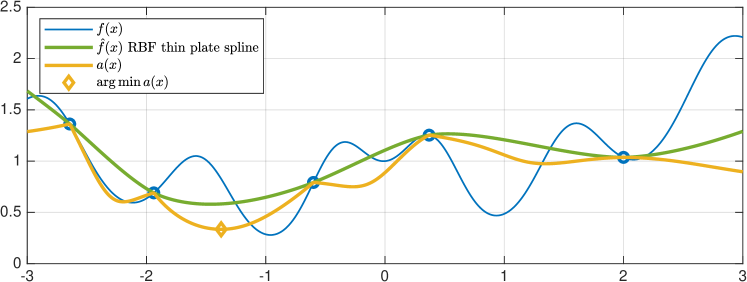
Figure 6: Plot of $\hat{f}(x)$ and acquisition function $a(x)$ with $\alpha=1$, $\delta=\frac{1}{2}$, thin plate spline RBF with $\epsilon_{\rm SVD}=10^{-6}$, for the scalar example as in Figure 1, with $w_{i}(x)$ as in (3a) and $f$ as in (6)

The following result, whose easy proof is reported in Appendix A, highlights a nice property of the acquisition function $a$:

Lemma 2

Function $a$ is differentiable everywhere on ${\mathbb{R}}^{n}$.

Problem (16) is a global optimization problem whose objective function and constraints are very easy to evaluate. It can be solved very efficiently using various global optimization techniques, either derivative-free [32] or, if $\mathcal{X}=\{x:g(x)\leq 0\}$ and $g$ is also differentiable, derivative-based. In case some components of vector $x$ are restricted to be integer, (16) can be solved by mixed-integer programming.

5 Global optimization algorithm

Algorithm 1, that we will refer to as GLIS (GLobal minimum using Inverse distance weighting and Surrogate radial basis functions), summarizes the proposed approach to solve the global optimization problem (1) using surrogate functions (either IDW or RBF) and the IDW acquisition function (15).

Algorithm 1 GLIS – Global optimization algorithm based on IDW-RBF surrogates

Input: Upper and lower bounds $(\ell,u)$, constraint set $\mathcal{X}$; number $N_{\rm init}$ of initial samples, number $N_{\rm max}\geq N_{\rm init}$ of maximum number of function evaluations; $\alpha,\delta\geq 0$, $\epsilon_{\rm SVD}>0$, $\epsilon_{\rm\Delta F}>0$.  

1. Tighten $(\ell,u)$ as in (11b);

2. Scale problem as in (12d);

3. Set $N\leftarrow N_{\rm init}$;

4. Generate $N$ random initial samples $X=[x_{1}\ \ldots\ x_{N}]^{\prime}$ using Latin hypercube sampling [28];

5. Compute $\hat{f}$ as in (7), (10c) (RBF function) or as in (5) (IDW function);

6. While $N<N_{\rm max}$ do

   1. Compute acquisition function $a$ as in (15);

   2. Solve global optimization problem (16) and get $x_{N+1}$;

   3. $N\leftarrow N+1$;

7. End.

    Output: Global optimizer $x^{*}=x_{N_{\rm max}}$.

As common in global optimization based on surrogate functions, in Step 0. Latin Hypercube Sampling (LHS) [28] is used to generate the initial set $X$ of samples in the given range $\ell,u$. Note that the generated initial points may not satisfy the inequality constraints $x\in\mathcal{X}$. We distinguish between two cases:

1. the objective function $f$ can be evaluated outside the feasible set $\mathcal{F}$;

2. $f$ cannot be evaluated outside $\mathcal{F}$.

In the first case, initial samples of $f$ falling outside $\mathcal{F}$ are still useful to define the surrogate function and can be therefore kept. In the second case, since $f$ cannot be evaluated at initial samples outside $\mathcal{F}$, a possible approach is to generate more than $N_{\rm init}$ samples and discard the infeasible ones before evaluating $f$. For example, the author of [6] suggests the simple method reported in Algorithm 2. This requires the feasible set $\mathcal{F}$ to be full-dimensional. In case of linear inequality constraints $\mathcal{X}=\{x:\ Ax\leq b\}$, full-dimensionality of the feasible set $\mathcal{F}$ can be easily checked by computing the Chebychev radius $r_{\mathcal{F}}$ of $\mathcal{F}$ via the LP [8]

$$\begin{array}[]{rl}r_{\mathcal{F}}=\max_{r,x}&r\\ \mathop{\rm s.t.}\nolimits&A_{i}x\leq b_{i}-\|A_{i}\|_{2}r,\ i=1,\ldots,q\\ &\ell_{i}+r\leq x_{i}\leq u_{i}-r,\ i=1,\ldots,n\end{array}$$ (17)

where in (17) the subscript $i$ denotes the $i$th row (component) of a matrix (vector). The polyhedron $\mathcal{F}$ is full dimensional if and only if $r_{\mathcal{F}}>0$. Clearly, the smaller the ratio between the volume of $\mathcal{F}$ and the volume of the bounding box $B_{\ell_{g},u_{g}}$, the larger on average will be the number of samples generated by Algorithm 2.

Note that, in alternative to LHS, the IDW function (14) could be also used to generate $N_{\rm init}$ feasible points by solving

$$x_{N+1}=\max_{x\in\mathcal{F}}z(x)$$

for $N=1,\ldots,N_{\rm init}-1$, for any $x_{1}\in\mathcal{F}$.

Algorithm 2 Latin hypercube sampling with constraints

Input: Upper and lower bounds $(\ell,u)$ for $x$ and inequality constraint function $g:{\mathbb{R}}^{n}\to{\mathbb{R}}^{q}$, defining a full dimensional set $\mathcal{F}=\{x\in{\mathbb{R}}^{n}:\ \ell\leq x\leq u,g(x)\leq 0\}$; number $N_{\rm init}$ of initial samples.  

1. $N\leftarrow N_{\rm init}$; $N_{k}\leftarrow 0$;

2. While $N_{k}<N_{\rm init}$ do

   1. Generate $N$ samples using Latin hypercube sampling;

   2. $N_{k}\leftarrow$ number of samples satisfying $x\in\mathcal{X}$;

   3. If $N_{k}<N_{\rm init}$ then increase $N$ by setting

      $$N\leftarrow\left\{\begin{array}[]{ll}\lceil\min\{20,1.1\frac{N_{\rm init}}{N_{k}}\}N\rceil&\mbox{if}\ N_{k}>0\\ 20N&\mbox{otherwise}\end{array}\right.$$

3. End.

    Output: $N_{\rm init}$ initial samples $X=[x_{1}\ \ldots\ x_{N_{\rm init}}]^{\prime}$ satisfying $\ell\leq x_{i}\leq u$, $x\in\mathcal{X}$.

The examples reported in this paper use the Particle Swarm Optimization (PSO) algorithm [41] to solve problem (16) at Step 0.0..2, although several other global optimization methods such as DIRECT [22] or others [18, 32] could be used in alternative. Inequality constraints $\mathcal{X}=\{x:\ g(x)\leq 0\}$ can be handled as penalty functions, for example by replacing (16) with

$$x_{N+1}=\arg\min_{\ell\leq x\leq u}a(x)+\rho\Delta F\sum_{i=1}^{q}\max\{g_{i}(x),0\}^{2}$$ (18)

where in (18) $\rho\gg 1$. Note that due to the heuristic involved in constructing function $a$, it is not crucial to find global solutions of very high accuracy when solving problem (16).

The exploration parameter $\alpha$ promotes visiting points in $[\ell,u]$ where the function surrogate has largest variance, $\delta$ promotes instead pure exploration independently on the surrogate function approximation, as it is only based on the sampled points $x_{1},\ldots,x_{N}$ and their mutual distance. For example, if $\alpha=0$ and $\delta\gg 1$ Algorithm 1 will try to explore the entire feasible region, with consequent slower detection of points $x$ with low cost $f(x)$. On the other hand, setting $\delta=0$ will make GLIS proceed only based on the function surrogate and its variance, that may lead to miss regions in $[\ell,u]$ where a global optimizer is located. For $\alpha=\delta=0$, GLIS will proceed based on pure minimization of $\hat{f}$ that, as observed earlier, can easily lead to converge away from a global optimizer.

Figure 7 shows the first six iterations of the GLIS algorithm when applied to minimize the function $f$ given in (6) in $[-3,3]$ with $\alpha=1$, $\delta=0.5$.

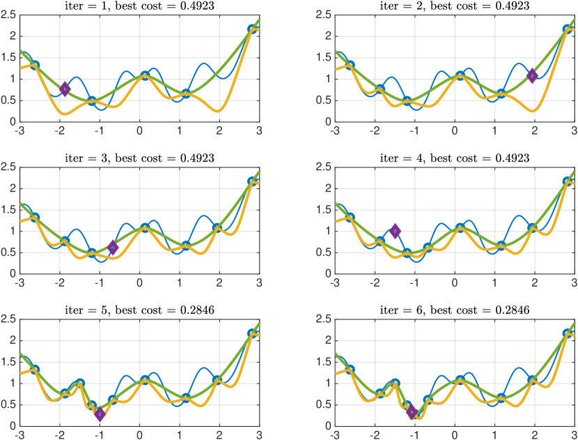
Figure 7: GLIS steps when applied to minimize the function $f$ given in (6) using the same settings as in Figure 6 and $\epsilon_{\rm SVD}=10^{-6}$. The plots show function $f$ (blue), its samples $f_{i}$ (blue circles), the thin plate spline interpolation $\hat{f}$ with $\epsilon=0.01$ (green), the acquisition function $a$ (yellow), and the minimum of the acquisition function reached at $x_{N+1}$ (purple diamond)

5.1 Computational complexity

The complexity of Algorithm 1, as a function of the number $N_{\rm max}$ of iterations and dimension $n$ of the optimization space and not counting the complexity of evaluating $f$, depends on Steps 0.0..1 and 0.0..2. The latter depends on the global optimizer used to solve Problem (16), which typically depends heavily on $n$. Step 0.0..1 involves computing $N_{\rm max}(N_{\rm max}-1)$ RBF values $\phi(\epsilon d(x_{i},x_{j}))$, $i,j=1,\ldots,N_{\rm max}$, $j\neq i$, compute the SVD decomposition of the $N\times N$ symmetric matrix $M$ in (10a), whose complexity is $O(N^{3})$, and solve the linear system in (10a) ($O(N^{2})$) at each step $N=N_{\rm init},\ldots,N_{\rm max}$.

6 Numerical tests

In this section we report different numerical tests performed to assess the performance of the proposed algorithm (GLIS) and how it compares to Bayesian optimization (BO). For the latter, we have used the off-the-shelf algorithm bayesopt implemented in the Statistics and Machine Learning Toolbox for MATLAB [39], based on the lower confidence bound as acquisition function. All tests were run on an Intel i7-8550 CPU @1.8GHz machine. Algorithm 1 was run in MATLAB R2019b in interpreted code. The PSO solver [42] was used to solve problem (18).

6.1 GLIS optimizing its own parameters

We first use GLIS to optimize its own hyperparameters $\alpha$, $\delta$, $\epsilon$ when solving the minimization problem with $f(x)$ as in (6) and $x\in[-3,3]$. In what follows, we use the subscript $()_{H}$ to denote the parameters/function used in the execution of the outer instance of Algorithm 1 that is optimizing $\alpha$, $\delta$, $\epsilon$. To this end, we solve the global optimization problem (1) with $x=[\alpha\ \delta\ \epsilon]^{\prime}$, $\ell_{H}=[0\ 0\ 0.1]^{\prime}$, $u_{H}=[3\ 3\ 3]^{\prime}$, and

$$f_{H}(x)=\sum_{i=1}^{N_{t}}\sum_{h=0}^{N_{\rm max}/2}(h+1)\min\{f(x_{i,1}),\ldots,f(x_{i,N_{\rm max}/2+h})\}$$ (19)

where $f$ is the scalar function in (6) that we want to minimize in $[-3,3]$, the $\min$ in (19) provides the best objective value found up to iteration $N_{\rm max}/2+h$, the term $(h+1)$ aims at penalizing high values of the best objective the more the later they occur during the iterations, $N_{t}=20$ is the number of times Algorithm 1 is executed to minimize $f_{H}$ for the same triplet $(\alpha,\delta,\epsilon)$, $N_{\rm max}=20$ is the number of times $f$ is evaluated per execution, $x_{i,N}$ is the sample generated by Algorithm 1 during the $i$th run at step $N$, $i=1,\ldots,N_{t}$, $N=1,\ldots,N_{\rm max}$. Clearly (19) penalizes failure to convergence close to the global optimum $f^{*}$ in $N_{\rm max}$ iterations without caring of how the algorithm performs during the first $N_{\rm max}/2-1$ iterations.

In optimizing (19), the outer instance of Algorithm 1 is run with $\alpha_{H}=1$, $\delta_{H}=0.5$, $\epsilon_{H}=0.5$, $N_{\rm init,H}=8$, $N_{\rm max,H}=100$, and PSO as the global optimizer of the acquisition function. The RBF inverse quadratic function is used in both the inner and outer instances of Algorithm 1. The resulting optimal selection is

$$\alpha=0.8215,\ \delta=2.6788,\ \epsilon=1.3296$$ (20)

Figure 8 compares the behavior of GLIS (Algorithm 1) when minimizing $f(x)$ as in (6) in $[-3,3]$ with tentative parameters $\alpha=1$, $\delta=1$, $\epsilon=0.5$ and with the optimal values in (20).

Clearly the results of the hyper-optimization depend on the function $f$ which is minimized in the inner loop. For a more comprehensive and general optimization of GLIS hyperparameters, one could alternatively consider in $f_{H}$ the average performance with respect to a collection of problems instead of just one problem.

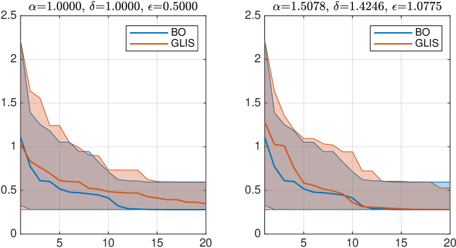
Figure 8: Minimization of $f(x)$ as in (6) in $[-3,3]$: tentative hyperparameters (left) and optimal hyperparameters (right)

6.2 Benchmark global optimization problems

We test the proposed global optimization algorithm on standard benchmark problems, summarized in Table 1. For each function the table shows the corresponding number of variables, upper and lower bounds, and the name of the example in [19] reporting the definition of the function. For lack of space, we will only consider the GLIS algorithm implemented using inverse quadratic RBFs for the surrogate, leaving IDW only for exploration.

As a reference target for assessing the quality of the optimization results, for each benchmark problem the optimization algorithm DIRECT [22] was used to compute the global optimum of the function through the NLopt interface [20], except for the ackley and stepfunction2 benchmarks in which PSO is used instead due to the slow convergence of DIRECT on those problems.

Algorithm 1 is run by using the RBF inverse quadratic function with hyperparameters obtained by dividing the values in (20) by the number $n$ of variables, with the rationale that exploration is more difficult in higher dimensions and it is therefore better to rely more on the surrogate function during acquisition. The threshold $\epsilon_{\rm SVD}=10^{-6}$ is adopted to compute the RBF coefficients in (10c). The number of initial samples is $N_{\rm init}=2n$.

For each benchmark, the problem is solved $N_{\rm test}=100$ times to collect statistically significant enough results. The last two columns of Table 1 report the average CPU time spent for solving the $N_{\rm test}=100$ instances of each benchmark using BO and GLIS. As the benchmark functions are very easy to compute, the CPU time spending on evaluating the $N_{\rm max}$ function values $F$ is negligible, so the time values reported in the Table are practically those due to the execution of the algorithms. Algorithm 1 (GLIS) is between 4.6 and 9.4 times faster than Bayesian optimization (about 7 times faster on average). The execution time of GLIS in Python 3.7 on the same machine, using the PSO package pyswarm (https://pythonhosted.org/pyswarm) to optimize the acquisition function, is similar to that of the BO package GPyOpt [38].

benchmark				function name
problem	$n$	$\ell$	$u$	[19]	BO[s]	GLIS [s]
ackley	2	$\left[\begin{smallmatrix}-5\\ -5\end{smallmatrix}\right]$	$\left[\begin{smallmatrix}5\\ 5\end{smallmatrix}\right]$	Ackley 1, $D=2$	29.39	3.13
adjiman	2	$\left[\begin{smallmatrix}-1\\ -1\end{smallmatrix}\right]$	$\left[\begin{smallmatrix}2\\ 1\end{smallmatrix}\right]$	Adjiman	3.29	0.68
branin	2	$\left[\begin{smallmatrix}-5\\ 0\end{smallmatrix}\right]$	$\left[\begin{smallmatrix}10\\ 15\end{smallmatrix}\right]$	Branin RCOS	9.66	1.17
camelsixhumps	2	$\left[\begin{smallmatrix}-5\\ -5\end{smallmatrix}\right]$	$\left[\begin{smallmatrix}5\\ 5\end{smallmatrix}\right]$	Camel - Six Humps	4.82	0.62
hartman3	3	$[0\ 0\ 0]^{\prime}$	$[1\ 1\ 1]^{\prime}$	Hartman 3	26.27	3.35
hartman6	6	$x_{i}\geq 0$	$x_{i}\leq 1$	Hartman 6	54.37	8.80
himmelblau	2	$\left[\begin{smallmatrix}-6\\ -6\end{smallmatrix}\right]$	$\left[\begin{smallmatrix}6\\ 6\end{smallmatrix}\right]$	Himmelblau	7.40	0.90
rosenbrock8	8	$\left[\begin{smallmatrix}-30\\ -30\end{smallmatrix}\right]$	$\left[\begin{smallmatrix}30\\ 30\end{smallmatrix}\right]$	Rosenbrock 1, $D=8$	63.09	13.73
stepfunction2	4	$x_{i}\geq-100$	$x_{i}\leq 100$	Step 2, $D=5$	11.72	1.81
styblinski-tang5	5	$x_{i}\geq-5$	$x_{i}\leq 5$	Styblinski-Tang, $n=5$	37.02	6.10

Table 1: Benchmark problems considered in the comparison. Last two columns: average CPU time spent on each benchmark for solving the $N_{\rm test}=100$ instances analyzed in Figure 9 by Bayesian optimization (BO) and GLIS (Algorithm 1)

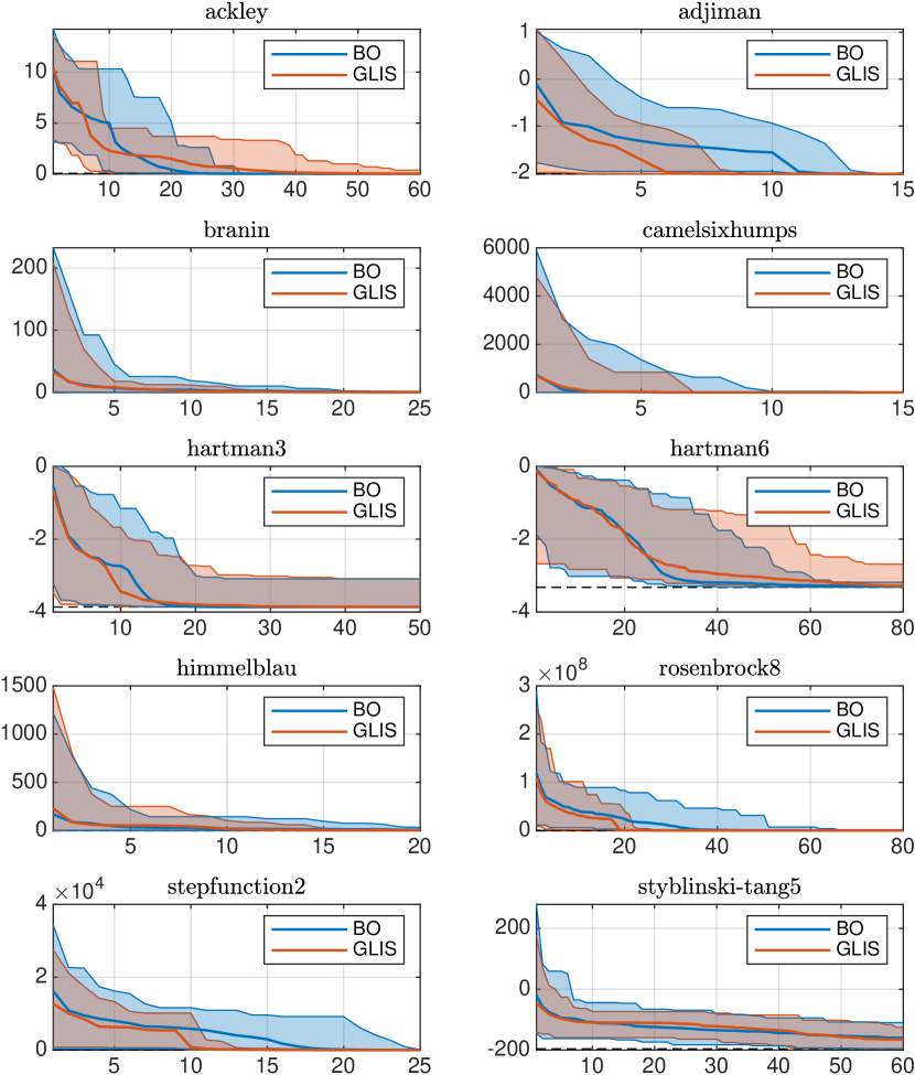
Figure 9: Comparison between Algorithm 1 (GLIS) and Bayesian optimization (BO) on benchmark problems. Each plot reports the average performance obtained over $N_{\rm test}=100$ runs as a function of the number of function evaluations, along with the band defined by the best- and worst-case instances

In order to test the algorithm in the presence of constraints, we consider the camelsixhumps problem and solve it under the following constraints

$$\begin{array}[]{ll}-2\leq x_{1}\leq 2,\quad-1\leq x_{2}\leq 1\\[10.00002pt] \left[\begin{smallmatrix}1.6295&1\\ -1&4.4553\\ -4.3023&-1\\ -5.6905&-12.1374\\ 17.6198&1\end{smallmatrix}\right]x\leq\left[\begin{smallmatrix}3.0786\\ 2.7417\\ -1.4909\\ 1\\ 32.5198\end{smallmatrix}\right],&x_{1}^{2}+(x_{2}+0.1)^{2}\leq 0.5\end{array}$$

Algorithm 1 is run with hyperparameters set by dividing by $n=2$ the values obtained in (20) and with $\epsilon_{\rm SVD}=10^{-6}$, $N_{\rm init}=2n$ for $N_{\rm max}=20$ iterations, with penalty $\rho=1000$ in (18). The results are plotted in Figure 10. The unconstrained two global minima of the function are located at $\left[\begin{smallmatrix}-0.0898\\ 0.7126\end{smallmatrix}\right]$, $\left[\begin{smallmatrix}0.0898\\ -0.7126\end{smallmatrix}\right]$.

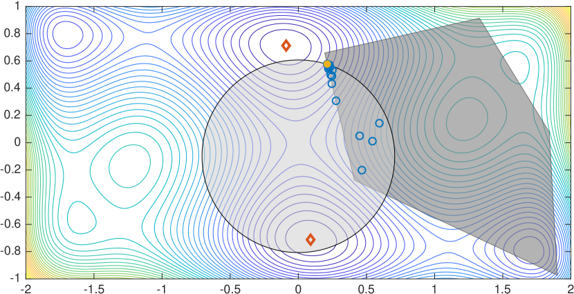
Figure 10: Constrained camelsixhumps problem: constrained minimum (yellow dot) and unconstrained global minima (red diamonds)

6.3 ADMM hyperparameter tuning for QP

The Alternating Direction Method of Multipliers (ADMM) [7] is a popular method for solving optimization problems such as the following convex Quadratic Program (QP)

$$\begin{array}[]{rl}\phi(\theta)=\min_{z}&\frac{1}{2}z^{\prime}Qz+(c+F\theta)^{\prime}z\\ \mathop{\rm s.t.}\nolimits&Az\leq b+S\theta\end{array}$$ (21)

where $z\in{\mathbb{R}}^{n}$ is the optimization vector, $\theta\in{\mathbb{R}}^{p}$ is a vector of parameters affecting the problem, and $A\in{\mathbb{R}}^{q\times n}$, $b\in{\mathbb{R}}^{q}$, $S\in{\mathbb{R}}^{q\times p}$, and we assume $Q=Q^{\prime}\succ 0$. Problems of the form (21) arise for example in model predictive control applications [2, 3], where $z$ represents a sequence of future control inputs to optimize and $\theta$ collects signals that change continuously at runtime depending on measurements and set-point values. ADMM can be used effectively to solve QP problems (21), see for example the solver described in [1]. A very simple ADMM formulation for QP is summarized in Algorithm 3.

Algorithm 3 ADMM for QP

Input: Matrices $Q,c,F,A,b,S$, parameter $\theta$, ADMM hyperparameters $\bar{\rho},\bar{\alpha}$, number $N$ of ADMM iterations.  

1. $M_{A}\leftarrow(\frac{1}{\bar{\rho}}Q+A^{\prime}A)^{-1}A^{\prime}$; $m_{\theta}\leftarrow(\frac{1}{\bar{\rho}}Q+A^{\prime}A)^{-1}(c+F\theta)$; $b_{\theta}\leftarrow b+S\theta$;

2. $s\leftarrow 0$, $u\leftarrow 0$;

3. for $i=1,\ldots,N$ do:

   1. $z\leftarrow M_{A}(s-u)-m_{\theta}$;

   2. $w\leftarrow\bar{\alpha}Az+(1-\bar{\alpha})s$;

   3. $s\leftarrow\min(w+u,b_{\theta})$;

   4. $u\leftarrow u+w-s$;

4. End.

    Output: Optimal solution $z^{*}=z$.

We consider a randomly generated QP test problem with $n=5$, $q=10$, $p=3$ that is feasible for all $\theta\in[-1,1]^{3}$, whose matrices are reported in Appendix B for reference. We set $N=100$ in Algorithm 3, and generate $M=2000$ samples $\theta_{i}$ uniformly distributed in $[-1,1]^{3}$. The aim is to find the hyperparameters $x=[\bar{\rho}\ \bar{\alpha}]^{\prime}$ that provide the best QP solution quality. This is expressed by the following objective function

$$f(x) = \log\left(\frac{1}{M}\sum_{j=1}^{M}\max\left\{\frac{\phi^{*}_{j}(x)-\phi^{*}(x)}{1+|\phi^{*}(x)|},0\right\}\right.$$ (22)

$$\left.+\bar{\beta}\max\left\{\max_{i}\left\{\frac{A_{i}z_{j}^{*}(x)-b_{i}-S_{i}x}{1+|b_{i}+S_{i}x|}\right\},0\right\}\right)$$

where $\phi^{*}_{j}(x)$, $z^{*}_{j}(x)$ are the optimal value and optimizer found at run $\#j$, respectively, $\phi^{*}(x)$ is the solution of the QP problem obtained by running the very fast and accurate ODYS QP solver [10]. The first term in (22) measures relative optimality, the second term relative violation of the constraints, and we set $\bar{\beta}=1$. Function $f$ in (22) is minimized for $\ell=\left[\begin{smallmatrix}0.01\\ 0.01\end{smallmatrix}\right]$ and $u=\left[\begin{smallmatrix}3\\ 3\end{smallmatrix}\right]$ using GLIS with the same parameters used in Section 6.2 and, for comparison, by Bayesian optimization. The test is repeated $N_{\rm test}=100$ times and the results are depicted in Figure 11. The resulting hyperparameter tuning that minimized the selected ADMM performance index (22) is $\bar{\rho}=0.1566$, $\bar{\alpha}=1.9498$.

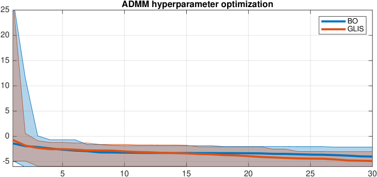
Figure 11: Hyperparameter optimization for ADMM

7 Conclusions

This paper has proposed an approach based on surrogate functions to address global optimization problems whose objective function is expensive to evaluate, possibly under constraints that are inexpensive to evaluate. Contrarily to Bayesian optimization methods, the approach is driven by deterministic arguments based on radial basis functions to create the surrogate, and on inverse distance weighting to characterize the uncertainty between the surrogate and the black-box function to optimize, as well as to promote the exploration of the feasible space. The computational burden associated with the algorithm is lighter then the one of Bayesian optimization while performance is comparable.

Current research is devoted to extend the approach to include constraints that are also expensive to evaluate, and to explore if performance can be improved by adapting the parameters $\alpha$ and $\delta$ during the search. Future research should address theoretical issues of convergence of the approach, by investigating assumptions on the black-box function $f$ and on the parameters $\alpha,\delta,\epsilon_{\rm SVD},\epsilon_{\rm\Delta F}$ of the algorithm, so to allow guaranteeing convergence, for example using the arguments in [15] based on the results in [40].

Appendix A Proofs

Proof of Lemma 1. Property P1 easily follows from (4). Property P2 also easily follows from the fact that for all $x\in{\mathbb{R}}^{n}$ the values $v_{j}(x)\in[0,1]$, $\forall j=1,\ldots,$ and $\sum_{j=1}v_{j}(x)=1$, so that

$$\min_{j}\{f_{j}\}=\sum_{j=1}^{N}v_{j}(x)\min_{j}\{f_{j}\}\leq\hat{f}(x)\leq\sum_{j=1}^{N}v_{j}(x)\max_{j}\{f_{j}\}=\max_{j}\{f_{j}\}$$

Regarding differentiability, we first prove that for all $i=1,\ldots,N$, functions $v_{i}$ are differentiable everywhere on ${\mathbb{R}}^{n}$, and that in particular $\nabla v_{i}(x_{j})=0$ for all $j=1,\ldots,N$. Clearly, functions $v_{i}$ are differentiable for all $x\not\in\{x_{1},\ldots,x_{N}\}$, $\forall i=1,\ldots,N$. Let $e_{h}$ be the $h$th column of the identity matrix of order $n$. Consider first the case in which $w_{i}(x)$ are given by (3b). The partial derivatives of $v_{i}$ at $x_{i}$ are

$$\frac{\partial v_{i}(x_{i})}{\partial x_{h}} = \lim_{t\rightarrow 0}\frac{1}{t}\left(\frac{w_{i}(x_{i}+te_{h})}{\sum_{j=1}^{N}w_{j}(x_{i}+te_{h})}-1\right)=\lim_{t\rightarrow 0}-\frac{\sum_{j\neq i}w_{j}(x_{i}+te_{h})}{t\sum_{j=1}^{N}w_{j}(x+te_{h})}$$

$$= \lim_{t\rightarrow 0}-\frac{\sum_{j\neq i}w_{j}(x_{i})}{t\frac{e^{-\|x_{i}+te_{h}-x_{i}\|^{2}}}{\|x_{i}+te_{h}-x_{i}\|^{2}}}=\lim_{t\rightarrow 0}-t\frac{\sum_{j\neq i}w_{j}(x_{i})}{e^{-t^{2}}}=0$$

and similarly at $x_{j}$, $j\neq i$ are

$$\frac{\partial v_{i}(x_{j})}{\partial x_{h}} = \lim_{t\rightarrow 0}\frac{1}{t}\left(\frac{w_{i}(x_{j}+te_{h})}{\sum_{j=1}^{N}w_{j}(x_{j}+te_{h})}-0\right)=\lim_{t\rightarrow 0}\frac{1}{t}\frac{w_{i}(x_{j})}{\frac{e^{-t^{2}}}{t^{2}}+\sum_{k\neq j}w_{k}(x_{j})}=0$$

In case $w_{i}(x)$ are given by (3a) differentiability follows similarly, with $e^{-t^{2}}$ replaced by 1. Therefore $\hat{f}$ is differentiable and

$$\nabla\hat{f}(x_{j})=\sum_{i=1}^{N}f_{i}\nabla v_{i}(x_{j})=0$$

 

Proof of Lemma 2. As by Lemma 1 functions $\hat{f}$ and $v_{i}$ are differentiable, $\forall i=1,\ldots,N$, it follows immediately that $s(x)$ is differentiable. Regarding differentiability of $z$, clearly it is differentiable for all $x\not\in\{x_{1},\ldots,x_{N}\}$, $\forall i=1,\ldots,N$. Let $e_{h}$ be the $h$th column of the identity matrix of order $n$. Consider first the case in which $w_{i}(x)$ are given by (3b). The partial derivatives of $z$ at $x_{i}$ are

$$\frac{\partial z(x_{i})}{\partial x_{h}} = \lim_{t\rightarrow 0}\frac{1}{t}\left(\frac{2}{\pi}\tan^{-1}\left(\frac{1}{\sum_{j=1}^{N}w_{j}(x_{i}+te_{h})}\right)-0\right)$$

$$= \lim_{t\rightarrow 0}\frac{2}{\pi t}\tan^{-1}\left(\frac{1}{\frac{e^{-t^{2}}}{t^{2}}+\sum_{j\neq i}w_{j}(x_{i})}\right)=\lim_{t\rightarrow 0}\frac{2}{\pi t}\tan^{-1}\left(\frac{t^{2}}{1+\sum_{j\neq i}w_{j}(x_{i})}\right)=0$$

In case $w_{i}(x)$ are given by (3a) differentiability follows similarly, with $e^{-t^{2}}$ replaced by 1. Therefore the acquisition function $a$ is differentiable for all $\alpha,\delta\geq 0$.  

Appendix B Matrices of parametric QP considered in Section 6.3

$$\begin{array}[]{l}Q=\footnotesize{\left[\begin{array}[]{rrrrrrr}&6.6067&-1.6361&2.8198&0.3776&3.1448\\ &-1.6361&0.9943&-0.9998&-0.4786&-0.5198\\ &2.8198&-0.9998&4.0749&0.2183&0.2714\\ &0.3776&-0.4786&0.2183&0.7310&0.1689\\ &3.1448&-0.5198&0.2714&0.1689&2.1716&\end{array}\right]}\quad c=\footnotesize{\left[\begin{array}[]{rrr}&-11.4795\\ &1.0487\\ &7.2225\\ &25.8549\\ &-6.6689&\end{array}\right]}\\ {}\\ A=\footnotesize{\left[\begin{array}[]{rrrrrrr}&-0.8637&-1.0891&-0.6156&1.4193&-1.0000\\ &0.0774&0.0326&0.7481&0.2916&-1.0000\\ &-1.2141&0.5525&-0.1924&0.1978&-1.0000\\ &-1.1135&1.1006&0.8886&1.5877&-1.0000\\ &-0.0068&1.5442&-0.7648&-0.8045&-1.0000\\ &1.5326&0.0859&-1.4023&0.6966&-1.0000\\ &-0.7697&-1.4916&-1.4224&0.8351&-1.0000\\ &0.3714&-0.7423&0.4882&-0.2437&-1.0000\\ &-0.2256&-1.0616&-0.1774&0.2157&-1.0000\\ &1.1174&2.3505&-0.1961&-1.1658&-1.0000&\end{array}\right]}\quad b=\footnotesize{\left[\begin{array}[]{rrr}&0.0838\\ &0.2290\\ &0.9133\\ &0.1524\\ &0.8258\\ &0.5383\\ &0.9961\\ &0.0782\\ &0.4427\\ &0.1067&\end{array}\right]}\\ {}\\ F=\footnotesize{\left[\begin{array}[]{rrrrr}&1.8733&8.4038&-6.0033\\ &-0.8249&-8.8803&4.8997\\ &-19.3302&1.0009&7.3936\\ &-4.3897&-5.4453&17.1189\\ &-17.9468&3.0352&-1.9412&\end{array}\right]}\quad S=\footnotesize{\left[\begin{array}[]{rrrrr}&2.9080&-0.3538&0.0229\\ &0.8252&-0.8236&-0.2620\\ &1.3790&-1.5771&-1.7502\\ &-1.0582&0.5080&-0.2857\\ &-0.4686&0.2820&-0.8314\\ &-0.2725&0.0335&-0.9792\\ &1.0984&-1.3337&-1.1564\\ &-0.2779&1.1275&-0.5336\\ &0.7015&0.3502&-2.0026\\ &-2.0518&-0.2991&0.9642&\end{array}\right]}\end{array}$$

References

- [1] G. Banjac, B. Stellato, N. Moehle, P. Goulart, A. Bemporad, and S. Boyd. Embedded code generation using the OSQP solver. In Proc. 56th IEEE Conf. on Decision and Control, pages 1906–1911, Melbourne, Australia, 2017. https://github.com/oxfordcontrol/osqp.
- [2] A. Bemporad. Model-based predictive control design: New trends and tools. In Proc. 45th IEEE Conf. on Decision and Control, pages 6678–6683, San Diego, CA, 2006.
- [3] A. Bemporad. A multiparametric quadratic programming algorithm with polyhedral computations based on nonnegative least squares. IEEE Trans. Automatic Control, 60(11):2892–2903, 2015.
- [4] A. Bemporad. Global optimization via inverse distance weighting. 2019. Available on arXiv at https://arxiv.org/pdf/1906.06498.pdf. Code available at http://cse.lab.imtlucca.it/~bemporad/idwgopt.
- [5] A. Bemporad and D. Piga. Active preference learning based on radial basis functions. 2019. Available on arXiv at http://arxiv.org/abs/1909.13049. Code available at http://cse.lab.imtlucca.it/~bemporad/idwgopt.
- [6] H.J. Blok. The lhsdesigncon MATLAB function, 2014. https://github.com/rikblok/matlab-lhsdesigncon.
- [7] S. Boyd, N. Parikh, E. Chu, B. Peleato, and J. Eckstein. Distributed optimization and statistical learning via the alternating direction method of multipliers. Foundations and Trends in Machine Learning, 3(1):1–122, 2011.
- [8] S. Boyd and L. Vandenberghe. Convex Optimization. Cambridge University Press, New York, NY, USA, 2004. http://www.stanford.edu/~boyd/cvxbook.html.
- [9] E. Brochu, V.M. Cora, and N. De Freitas. A tutorial on Bayesian optimization of expensive cost functions, with application to active user modeling and hierarchical reinforcement learning. arXiv preprint arXiv:1012.2599, 2010.
- [10] G. Cimini, A. Bemporad, and D. Bernardini. ODYS QP Solver. ODYS S.r.l. (https://odys.it/qp), September 2017.
- [11] A. Costa and G. Nannicini. Rbfopt: an open-source library for black-box optimization with costly function evaluations. Mathematical Programming Computation, 10(4):597–629, 2018.
- [12] R. Eberhart and J. Kennedy. A new optimizer using particle swarm theory. In Proceedings of the Sixth International Symposium on Micro Machine and Human Science, pages 39–43, Nagoya, 1995.
- [13] M. Feurer, A. Klein, K. Eggensperger, J.T. Springenberg, M. Blum, and F. Hutter. Auto-sklearn: Efficient and robust automated machine learning. In F. Hutter, L. Kotthoff, and J. Vanschoren, editors, Automated Machine Learning: Methods, Systems, Challenges, pages 113–134. Springer International Publishing, 2019.
- [14] M. Forgione, D. Piga, and A. Bemporad. Efficient calibration of embedded MPC. 2019. Submitted. Available at https://arxiv.org/abs/1911.13021.
- [15] H.-M. Gutmann. A radial basis function method for global optimization. Journal of Global Optimization, 19:201–2227, 2001.
- [16] N. Hansen and A. Ostermeier. Completely derandomized self-adaptation in evolution strategies. Evolutionary Computation, 9(2):159–195, 2001.
- [17] R.L. Hardy. Multiquadric equations of topography and other irregular surfaces. Journal of geophysical research, 76(8):1905–1915, 1971.
- [18] W. Huyer and A. Neumaier. Global optimization by multilevel coordinate search. Journal of Global Optimization, 14(4):331–355, 1999.
- [19] M. Jamil and X.-S. Yang. A literature survey of benchmark functions for global optimisation problems. Int. J. Mathematical Modelling and Numerical Optimisation, 4(2):150–194, 2013. https://arxiv.org/pdf/1308.4008.pdf.
- [20] S.G. Johnson. The NLopt nonlinear-optimization package. http://github.com/stevengj/nlopt.
- [21] D.R. Jones. A taxonomy of global optimization methods based on response surfaces. Journal of Global Optimization, 21(4):345–383, 2001.
- [22] D.R. Jones. DIRECT global optimization algorithm. Encyclopedia of Optimization, pages 725–735, 2009.
- [23] D.R. Jones, M. Schonlau, and W.J. Matthias. Efficient global optimization of expensive black-box functions. Journal of Global Optimization, 13(4):455–492, 1998.
- [24] V.R. Joseph and L. Kang. Regression-based inverse distance weighting with applications to computer experiments. Technometrics, 53(3):255–265, 2011.
- [25] H.J. Kushner. A new method of locating the maximum point of an arbitrary multipeak curve in the presence of noise. Journal of Basic Engineering, 86(1):97–106, 1964.
- [26] G. Matheron. Principles of geostatistics. Economic geology, 58(8):1246–1266, 1963.
- [27] D.B. McDonald, W.J. Grantham, W.L. Tabor, and M.J. Murphy. Global and local optimization using radial basis function response surface models. Applied Mathematical Modelling, 31(10):2095–2110, 2007.
- [28] M.D. McKay, R.J. Beckman, and W.J. Conover. Comparison of three methods for selecting values of input variables in the analysis of output from a computer code. Technometrics, 21(2):239–245, 1979.
- [29] D. Piga, M. Forgione, S. Formentin, and A. Bemporad. Performance-oriented model learning for data-driven MPC design. IEEE Control Systems Letters, 2019. Also in Proc. 58th IEEE Conf. Decision and Control, Nice (France), 2019. https://arxiv.org/abs/1904.10839.
- [30] M.J.D. Powell. The NEWUOA software for unconstrained optimization without derivatives. In Large-scale nonlinear optimization, pages 255–297. Springer, 2006.
- [31] R.G. Regis and C.A. Shoemaker. Constrained global optimization of expensive black box functions using radial basis functions. Journal of Global optimization, 31(1):153–171, 2005.
- [32] L.M. Rios and N.V. Sahinidis. Derivative-free optimization: a review of algorithms and comparison of software implementations. Journal of Global Optimization, 56(3):1247–1293, 2013.
- [33] S. Rippa. An algorithm for selecting a good value for the parameter c in radial basis function interpolation. Advances in Computational Mathematics, 11(2-3):193–210, 1999.
- [34] J. Sacks, W.J. Welch, T.J. Mitchell, and H.P. Wynn. Design and analysis of computer experiments. Statistical Science, pages 409–423, 1989.
- [35] B. Shahriari, K. Swersky, Z. Wang, R.P. Adams, and N. De Freitas. Taking the human out of the loop: A review of Bayesian optimization. Proceedings of the IEEE, 104(1):148–175, 2015.
- [36] D. Shepard. A two-dimensional interpolation function for irregularly-spaced data. In Proc. ACM National Conference, pages 517–524. New York, 1968.
- [37] J. Snoek, H. Jasper, and R.P. Adams. Practical Bayesian optimization of machine learning algorithms. In Advances in neural information processing systems, pages 2951–2959, 2012.
- [38] The GPyOpt authors. GPyOpt: A Bayesian optimization framework in Python. http://github.com/SheffieldML/GPyOpt, 2016.
- [39] The Mathworks, Inc. Statistics and Machine Learning Toolbox User’s Guide, 2019. https://www.mathworks.com/help/releases/R2019a/pdf_doc/stats/stats.pdf.
- [40] A. Törn and A. Žilinskas. Global Optimization, volume 350. Springer, 1989.
- [41] A.I.F. Vaz and L.N. Vicente. A particle swarm pattern search method for bound constrained global optimization. Journal of Global Optimization, 39(2):197–219, 2007.
- [42] A.I.F. Vaz and L.N. Vicente. PSwarm: A hybrid solver for linearly constrained global derivative-free optimization. Optimization Methods and Software, 24:669–685, 2009. http://www.norg.uminho.pt/aivaz/pswarm/.
- [43] D. Whitley. A genetic algorithm tutorial. Statistics and computing, 4(2):65–85, 1994.