RECAL: Reuse of Established CNN classifer Apropos unsupervised Learning paradigm

Abstract

Recently, clustering with deep network framework has attracted attention of several researchers in the computer vision community. Deep framework gains extensive attention due to its efficiency and scalability towards large-scale and high-dimensional data. In this paper, we transform supervised CNN classifier architecture into an unsupervised clustering model, called RECAL, which jointly learns discriminative embedding subspace and cluster labels. RECAL is made up of feature extraction layers which are convolutional, followed by unsupervised classifier layers which is fully connected. A multinomial logistic regression function (softmax) stacked on top of classifier layers. We train this network using stochastic gradient descent (SGD) optimizer. However, the successful implementation of our model is revolved around the design of loss function. Our loss function uses the heuristics that true partitioning entails lower entropy given that the class distribution is not heavily skewed. This is a trade-off between the situations of “skewed distribution” and “low-entropy”. To handle this, we have proposed classification entropy and class entropy which are the two components of our loss function. In this approach, size of the mini-batch should be kept high. Experimental results indicate the consistent and competitive behavior of our model for clustering well-known digit, multi-viewed object and face datasets. Morever, we use this model to generate unsupervised patch segmentation for multi-spectral LISS-IV images. We observe that it is able to distinguish built-up area, wet land, vegetation and water-body from the underlying scene.

1 Introduction

Clustering of large scale data is an active area of research in deep learning and big-data domain. It has gained significant attention as labeling data is costly and anomalous in real-world data. For example, getting ground truths for satellite imagery is difficult. A few disaster management applications suffer from that. Nevertheless, clustering algorithms have been studied widely. But, its performance drops drastically when it encounters high dimensional data. Also, their time-complexity increases dramatically. To handle curse of dimensionality, original data space is projected into low dimensional manifold and clustering is applied using them with standard algorithms on that new manifold. However, this approach fails when number of samples reaches to millions or billions. To cope up with the situation, several deep architecture based clustering approaches have been proposed in recent years. Most of them are CNN or feed-forward based auto encoder architecture [22, 3, 23, 1], embedded with simple, k-means like, clustering algorithm. These models have the tendency of learning features of the dataset and their corresponding cluster labels jointly. They employ a heuristic for clustering and use it along with the reconstruction loss function for training the model. Therefore, the bottleneck is to get initial clusters to accommodate clustering objective function in the loss function. The intuitive choice for the above problem is to train well-known auto-encoder model with reconstruction loss to generate new embedding subspace. Then, best known clustering algorithm is employed on that subspace to generate clusters [3]. Thereafter, new model is ready to train using two components of the loss function. However, another choice is to employ k-means like algorithm to get initial cluster labels. Other than auto-encoders, there are stacked convolutional layer based deep architecture exist [8]. However, they pre-trained their model with large-scale ImageNet dataset in order to use clustering objective function. It is to be noted that if the model architecture is similar to well-known classifiers architecture like AlexNet [10], VGG [16], ResNet [6], DenseNet [9] then learned parameters on those layers are eventually transferred. However, pre-training is only an approach of initializing the model parameters as this can not fit the data distribution of the dataset under consideration. Also, it is speeding up the convergence of iterations for real time training. To put it in a nutshell, the existing unsupervised deep approaches have following pitfalls: 1) training the network from scratch, and 2) obtaining initial cluster labels. To address the above mentioned pitfalls, we propose a deep clustering algorithm which does not require any initial cluster labels. In this paper, we consider the following two issues:

1. Can we utilize features generated from well-known pre-trained deep networks to develop clustering algorithm such that computational cost and memory requirement be reduced?

2. Can we perform clustering of these feature vectors under the same deep learning framework in absence of any information on labeling of these data?

In recent years, AlexNet [10], VGG [16], ResNet [6], DenseNet [9] receive high popularity in ImageNet challenge. Thus, it motivates us to choose one of the networks which have the capability of extracting good feature representatives. However, these networks are supervised. Hence, they can not be used in the scenario where no label is present. In this paper, we propose a loss function which enable the unsupervised labeling of data using these networks. For the purpose of illustration, we have chosen typically VGG-16 with batch normalization in our experiments. Also, we replace all fully connected and following layers by a single fully connected layer followed by batch normalization and ReLU layers. Our loss function is formulated using following entropy based clustering heuristics:

1. For a true partitioning, low entropy is desirable. This demands highly skewed probability distribution for a sample to be assigned to a cluster.

2. Any random partitioning than the actual one should lead to higher entropy, given the class distribution is not heavily skewed. For example, when all the feature vectors form trivially a single cluster, the distribution becomes highly skewed. In this case, though the entropy is zero, it does not reflect any meaningful information regarding partitioning.

There is a trade-off between these two factors. We propose a loss function for the network which takes into account these two factors for a given number of clusters. To summarize, the major contributions of our work are:

1. We propose a simple but effective approach to reuse well-known supervised deep architectures in an unsupervised learning paradigm.

2. We formulate an entropy based loss function to guide clustering and deep representation learning in a single framework that can be transferred to other tasks and datasets.

3. Our experimental results show that the proposed framework is consistent and competitive irrespective of different datasets.

4. Finally, we use this network in remote sensing domain to provide segmentation for multi-spectral images.

2 Approach

2.1 Notation

We represent an image set with $n$ images by $X=\{x_{1},\cdots,x_{n}\}$ where each sample $x_{i}$ represents an image of resolution $n_{1}\times n_{2}$. The clustering task is to group image set $X$ into $K$ clusters $Y=\{y_{1},\cdots y_{K}\}$. Using embedding function $f_{\theta}\mathrel{\mathop{\mathchar 58\relax}}X\rightarrow Z$, we transform raw image samples $X$ into its embedding subspace $Z=\{z_{1},\cdots,z_{n}\}$ where $z_{i}\in\mathbb{R}^{d}$. We estimate posterior probability $\mathbb{P}(Y|Z)$ and use Eq. 1 to assign each of the samples to one of $K$ cluster labels.

$$\hat{k}_{x_{i}}=\underset{k}{\operatorname*{arg\,max}}~{}\mathbb{P}(y_{k}|z)$$ (1)

However, we reuse well-known CNN network architecture to transform raw images into its embedded subspace. It is well-known that transfer learning expedites the process of learning new distribution. Hence, we may transfer learned weights of those networks in the beginning. Additionally, softmax function is used to learn $\mathbb{P}(Y|Z)$. Section 3.4 describes detailed architecture of our model.

2.2 Unsupervised Training Criterion

Motivation: Designing a loss function for unsupervised classification is highly influenced by the concept of “structuredness” and “diversity” of the dataset. Data can be well predicted if it belongs to a uniform distribution. In information theory, this “structuredness” is quantified by low entropy. On the other hand, multi class environment is characterized by “diversity” in data, which increases entropy of the dataset. A clustering algorithm becomes vulnerable when it produces highly skewed partition. Thereby, it witnesses low entropy. Therefore, it is desirable that an algorithm should report low entropy for a partition only when it is non-skewed.
Deep Network Scenario: We discuss this issue in the context of deep architecture. In general, deep networks are trained by the dataset which is divided into mini-batches. They accumulate losses incurred by each mini-batch and update the parameters of the network by incorporating the gradient of the loss function. We consider that a data is well classified by the network when the probability that it corresponds to a particular class out of $K$ classes, is near about 1. Therefore, it estimates low entropy. To accomplish it, classification entropy ($H_{\Phi}$) is designed. However, skewed partitioning is reduced by enforcing “diversity” in the mini-batch. The underlying intuition is that more the number of distinct representatives the architecture experiences in a mini-batch, better it learns the grouping. To accomplish it, class entropy ($H_{\Psi}$) is designed. Therefore, the aim is to maximize the class entropy while minimizing classification entropy.
Mathematical Formulation: In our model, we have feature extraction layers and classification layers. Feature extraction layers provide the mapping from input image space to feature embedded space $f_{\theta_{1}}\mathrel{\mathop{\mathchar 58\relax}}X\rightarrow Z$. However Classification layers provide the mapping of feature embedded space to cluster labels space, i.e.$f_{\theta_{2}}\mathrel{\mathop{\mathchar 58\relax}}Z\rightarrow R$. We are interested in knowing the probability that the $m^{th}$ sample belongs to $l^{th}$ class, which is denoted as $p_{ml}$. i.e.

$$p_{ml}=P(y_{m}=l|R)=\frac{exp({r_{ml}})}{\sum_{j=1}^{K}exp({r_{mj}})}$$ (2)

We design our loss function ($L$) for unsupervised classification with aforesaid motivation as follows :

$$\begin{array}[]{lll}L&=&\lambda H_{\Phi}-H_{\Psi}\\ \\ H_{\Phi}&=&-\frac{1}{M}\sum_{m=1}^{M}\sum_{l=1}^{K}p_{ml}\log(p_{ml})\\ \\ H_{\Psi}&=&-\sum_{l=1}^{K}p_{l}\log(p_{l})\\ \\ p_{l}&=&\frac{\sum_{m=1}^{M}(p_{ml})}{\sum_{l=1}^{K}\sum_{m=1}^{M}(p_{ml})}\\ \\ \end{array}$$ (3)

where $\lambda$ weighs loss function $L$.

2.3 Implementation Bottleneck

In our work, mini-batch size is a prime factor for successful implementation of our proposition. It is important that network should see all possible cluster representatives in one go. To maintain this criterion, mini batch size should be sufficiently large. However, with the constrained size of GPU, it could be hard to train network with a large batch-size. Therefore, Algorithm 1 may not be reliable for assigning efficient cluster labels to the input samples. To deal with such bottleneck, we employ a strategy to increase the mini-batch size. We can store losses, incurred by $t-1$ mini-batches using only $K+1$ variable. Therefore, $t^{th}$ mini-batch will accumulate previous semi processed losses and generate loss for all the samples that network visits till now. Then, it back propagates the accumulated loss in the network. With this strategy, it is possible to execute our algorithm even in the GPU with constrained memory. Algorithm 2 depicts the strategy.

1

Input : 

X=Collection of Image Data

K=Target number of cluster

B= Batch Size

Output : 

$Y^{*}$ : image labels

$\theta^{*}$ : CNN parameters

2

3Initialize $\theta$, optimizer=(SGD, lr=0.0001)

4 repeat

5       foreach minibatch do

6             Compute $\mathbb{P}(Y|Z)$ by forward propagation using $\theta$.

7             compute Loss= $\lambda H_{\Phi}-H_{\Psi}$ using Eq.3.

8             Update $\theta$ by back propagation.

9       end foreach

10      

11until converged;

Algorithm 1 Joint optimization on $y$ and $\theta$

1

Input : 

X=Collection of Image Data

K=target number of cluster

M= Number of samples in each mini-batch

t=number of mini-batches in one pass

Output : 

$Y^{*}$ : image labels

$\theta^{*}$ : CNN parameters

2

3Initialize $\theta$, SGD=(lr,momentum),mini-batch-size=0

4 repeat

5       foreach minibatch ($B$) do

6            

7            mini-batch-size+=size of $B$.

8             Compute $\mathbb{P}(Y|Z)$ by forward propagation using $\theta$.

9             if t mini-batches visited then

10                  

11                  $h_{\phi}=h_{\phi}+\sum_{m=1}^{M}\sum_{l=1}^{K}p_{ml}\log(p_{ml})$

12                   $H_{\Phi}=h_{\phi}/$mini-batch-size

13                   $h_{\psi}=h_{\psi}+\sum_{m=1}^{M}(p_{ml})$

14                   $p_{l}=\frac{(h_{\psi}))}{\sum_{k=1}^{K}(h_{\psi})}$

15                   $H_{\Psi}=-\sum_{l=1}^{K}p_{l}\log(p_{l})$

16                   Loss= $\lambda H_{\Phi}-H_{\Psi}$

17                   Update $\theta$ by back propagation.

18                   mini-batch-size=0

19            else

20                   $h_{\phi}=h_{\phi}+\sum_{m=1}^{M}\sum_{l=1}^{K}p_{ml}\log(p_{ml})$

21                   $h_{\psi}=h_{\psi}+\sum_{m=1}^{M}(p_{ml})$

22                   store $h_{\phi}$, $h_{\psi}.$

23             end if

24            

25       end foreach

26      

27until converged;

Algorithm 2 Joint optimization on $y$ and $\theta$ for large size of minibatch beyond the available GPU capacity

3 Experiments

In this section, we first compare RECAL with state-of-the-art clustering methods on several bench-mark image datasets. Then, we run k-means clustering algorithm on our learned deep representations. Finally, we analyze the performance of RECAL model on unsupervised segmentation task on multi-spectral LISS-IV images.

3.1 Alternative Clustering Models

We compare our model with several baseline and deep models, including k-means, normalized cuts (NCuts) [14], self-tuning spectral clustering (SC-ST) [25], large-scale spectral clustering (SC-LS) [2],  graph degree linkage-based agglomerative clustering (AC-GDL) [26], agglomerative clustering via path integral (AC-PIC) [27], local discriminant models and global integration (LDMGI) [24], NMF with deep model (NMF-D) [19], task-specific clustering with deep model (TSC-D) [20], deep embedded clustering (DEC)[22], joint unsupervised learning (JULE) [23] and deep embedded regularized clustering (DEPICT) [3] for unsupervised clustering.

Table 1: Description of Datasets

Dataset	MNIST-full	USPS	COIL-20	COIL-100	U-Mist	CMU-PIE	YTF
#Samples	70000	9298	1440	7200	575	2856	10000
#Categories	10	10	20	100	20	68	41
Image Size	28$\times$ 28	16 $\times$ 16	128 $\times$ 128	128 $\times$ 128	112 $\times$ 92	32 $\times$ 32	55 $\times$ 55

3.2 Dataset

We have chosen different types of datasets to show consistent behavior of our model towards accomplishing clustering. As, we are examining unsupervised models, we concatenate training and test datasets whenever applicable. MNIST-full [11]: It contains monochrome images of handwritten digits. USPS: It is a handwritten digits dataset from the US postal services. COIL-20 and COIL-100 [12]: They are databases of multi-view objects. UMist [5]: It includes face images of 20 people. CMU-PIE [15]: It includes face images of 4 different facial expressions. Youtube-Face (YTF) [21]: We follow an experimental set up for this dataset as in  [23, 3]. We select the first 41 subjects of YTF dataset. Faces inside images are first cropped and then resized to 55 by 55 sizes. A brief description of these datasets is provided in Table 1.

3.3 Evaluation Metric

We follow current literature which uses normalized mutual information (NMI) [7] as evaluation criteria for clustering algorithms. NMI evaluates the similarity between two labels of same dataset in normalized form (0,1). However, $0$ implies no correlation and 1 shows perfect correlation between two labels. We use predicted labels (by the model) and the ground truth labels to estimate NMI.

3.4 Implementation Details

We adopt feature extraction layers of VGG16 [16] with batch normalization and use the weights of the original network trained with ImageNet as a starting point. However, we consider a fully connected layer followed by a batch normalization and a ReLU layer for unsupervised labeling (equivalent classification layers). We stacked classification layers on top of feature extraction layers of VGG16. For USPS dataset, we decapitate feature layers of VGG16 to get an output of size $1\times 1$, otherwise, we use all feature layers of VGG16. Consequently, we normalize the image intensities using Eq. 4 where ($\mu$) and ($\sigma$) are mean and standard deviation of the given dataset, respectively. Moreover, we use stochastic gradient discent (SGD) as our optimization method with the learning rate=0.0001 and momentum=0.9. The weights of fully connected layer is initialized by Xavier approach [4]. Pre-trained models may not generate useful features to obtain a good clustering for the target dataset. Hence, fine-tuning is required. Pre-trained models not only expedite the process of convergence in fine-tuning but, it helps to provide a global solution instead of a local one.

$$\hat{x}=\frac{x-\mu}{\sigma}$$ (4)

3.5 Quantitative Comparison

We show NMI for every method on various datasets. Experimental results are averaged over 3 runs. We borrowed best results from either original paper or [23] if reported on a given dataset. Otherwise, we put dash marks (-) without reporting any result. We report our results in two parts: 1) the clustering labels predicted by our network after training it for several epochs; 2) the clustering results obtained by running k-means clustering algorithm on learned representation by our network. Table 6 reports the clustering metric, normalized mutual information (NMI), of the comparative algorithms along with RECAL on the aforementioned datasets. We have transferred weights of feature layers of VGG-16 (trained with ImageNet) to the feature layers of RECAL and classification layers are initialized with Xavier’s approach. As shown, RECAL perform competitively and consistently. It should be noted that hyper parameter tuning using labeled samples is not feasible always in real world clustering task. DEPICT has already shown an approach of not using supervised signals. However, their approach is dependent on other clustering algorithm. Hence, our algorithm is an independent and significantly better clustering approach for handling real world large scale dataset. Interestingly, clustering results on learned representatives produce better outcome as shown in Table 7. It indicates that our method can learn more discriminative feature representatives compared to image intensity. Notably, our learned representation is much better than JULE [23] for multi-viewed objects and digit dataset where their clustering result by their model, produce perfect NMI on COIL-20. However, our method performs poorly on face datasets. Also, Table 6 suggests that learned features are much distinctive compared to the features obtained by VGG-16 model trained with ImageNet.We have executed our code on a machine with GeForce GTX 1080 Ti GPU.

4 Multi-spectral image segmentation

For illustrating usefulness of this approach, we consider application of this method for unsupervised labeling of pixels in an image. We experiment with satellite multi-spectral images. We have observed that very tiny patches may be a representative of a pure class. With this assumption, we split the pre-processed satellite image into small patches (e.g, $32\times 32$ or $16\times 16$ or $8\times 8$) with strides of $k$ (e.g, $16$ or $8$) pixels. However, we decapitate the feature layers of VGG-16 from its tail such that size of the feature (not output of whole model) for an input patch of $8\times 8$ is $1\times 1$. Otherwise, there is no change in the network architecture. We do our experiments with other large size patches on this decapitated version of the network.

4.1 Description of Dataset

For our experiments, we have used images captured by Linear Imaging Self Scanner LISS-IV sensor of RESOURCESAT-2. Table 2 illustrates the specifications of LISS-IV sensor and scene details. It includes sensors, acquisition dates and other specification of the Indian Remote Sensing Resourcesat-2 mission. We have taken two scenes for our experiment. Scene information is shown in Table 3. Both scenes are captured by the same LISS-IV sensor on different dates. As field investigation is a crucial task and requires expertise, we have used Microsoft® BingTM maps for validation of our experiment.

Table 2: Specification of LISS-IV sensor and scene information

Description of Parameter	Details
Agency	NRSC
Satellite	Resourcesat 2
Sensor	LISS-IV
Swath (km)	70
Resolution (m)	5.8
Repetivity (days)	5
Qunatisation	10-bit
No of Bands	3
Spectral Bands ($\mu$)	Band 2 (0.52 - 0.59 ) Band 3 (0.62 - 0.68 ) Band 4 (0.77 - 0.86 )

Table 3: Description of the study area

Scene	Parameters	Details
Scene-1	Acquisition Date	25-NOV-2011
	Scene Center Lattitude	22.426371 N
	Scene Center Longitude	88.169285 E
Scene-2	Acquisition Date	10-APR-2017
	Scene Center Lattitude	23.615814 N
	Scene Center Longitude	87.400460 E

4.2 Description of Scene

Scene-1 covers an approximately 21 km $\times$ 23 km rectangle region located surrounding the city of Kolkata in West Bengal, India. This region mainly contains built-up areas, bare lands, vegetation (man made gardens, play grounds, small agricultural land etc), and water body. We have cropped small regions from the original data. On the other hand, Scene-2 is the whole dataset. It covers nearly 71 km $\times$ 86 km rectangle region located surrounding the place of Ranugunj, Durgapur, Panagarh, Dubrajpur etc. in West Bengal, India. However, this scene contains large hierarchy of classes. It contains built-up area, bare lands, vegetation (forest area, agricultural land, man made gardens etc.), water-body, coal mining area, etc. Moreover, built-up area covers a large area in Scene-1, whereas vegetation region predominates in Scene-2.

4.3 Pre-processing of dataset

In general, a sensor captures Earth’s surface radiance and this response is quantized into $n$-bit values. It is commonly called Digital Number (DN). However, to convert calibrated (DNs) to at-sensor radiance, two meta-parameters are used: known dynamic-range limits of the instrument and their corresponding pre-defined spectral radiance values. Meta files are provided by the satellite data provider. This radiance is then converted to top-of-atmosphere (ToA) reflectance by normalizing for solar elevation and solar spectral irradiance.

4.4 Results

In this experiment, we separately trained the model with the patches from Scene-1 and Scene-2 for $K=10$. Lets call it model-1 and model-2 respectively. We observe each segmented output from model-1 and model-2 separately. However, we check cross-dataset segmentation output which measures the robustness of the network. i.e, We use model-1 to generate the segmentation for scene-2 and vice versa. Notably, number of patches from Scene-1 and Scene-2 are approx. 0.2 million and 2.2 million respectively. Models took nearly 1-1.5 days for training. For Scene-1, our model has detected built-up area, vegetation and water-body distinctively among 10 classes. However, model-2 identifies vegetation, water body and wetland area. This is to be noted that model-2 predicts vegetation into three distinct classes. This result might be indicator of three types of vegetation in that location. We have shown models’ predictions and Microsoft® BingTM maps of the scenes in Fig 3, 4 and Fig 1, 2, respectively. Notably, Fig 3(a) and Fig 3(g) show different types of region for a particular class in two scenes: built-up area in Scene-1 and wetland in Scene-2. Many of previous researches [13, 17, 18] have reported similar characteristics of built-up area with wetland, farmland, etc. Similar false alarms persist in our experiment too. We use same color symbol for showing same cluster number in both scene-1 and scene-2 for the same model in Fig 3, 4.

4.4.1 Analysis

Experimental results reflect the generalization of model-1 and model-2 in various classes in Fig 3, 4. For example, Fig 3(a), 4(f) provide visually similar structure for water-body. We prepare a validation set using Microsoft® BingTM maps of that region. It shows 97% accuracy in identifying water-body in validation set. Taking visual consensus of two models, we are able to identify a few such structures for vegetation and wet land. For Scene-2 following pair of figures describe visually similar structure: (Fig 3(h), Fig 4(c)), (Fig 3(i), Fig 4(b)) and (Fig 3(g), Fig 4(e)). Similarly, (Fig 3(d), Fig 4(g)) and (Fig 3(e), Fig 4(h)) reveal similar visual structure in Scene-1. We measure consensus of two models using Jaccard similarity score as shown in Eq 5.

$$\text{\emph{ Jaccard similarity}}=\frac{\mathinner{\!\left\lvert M1\cap M2\right\rvert}}{\mathinner{\!\left\lvert M1\cup M2\right\rvert}}$$ (5)

where $M1$ and $M2$ represent pixels predicted by model-1 and model-2, respectively. Table-4 and Table-5 show the Jaccard similarity score for various identified classes in scene-1 and scene-2, respectively. We have shown upper triangular matrix in Table 4, 5 due to the symmetric nature of this score. We follow similar naming convention for denoting a particular class for a specific scene as shown in Fig 3, 4. However, further study is required for validating different classes with ground truth data, such as vegetation, wet land, built up areas, etc.

Table 4: Jaccard similarity score for different classes (as shown in Fig 3, 4) for scene-1

		Model-2
		cV1S1	cV2S1	cB2S1	cB1S1	cWBS1
Model-1	V1S1	0.545	0.004	0.004	0.002	0.004
	V2S1		0.299	0.015	0.014	0.001
	B1S1			0.243	0.105	0.007
	B2S1				0.211	0.004
	WBS1					0.721

Table 5: Jaccard similarity score for different classes (as shown in Fig 3, 4) for scene-2

		Model-1
		cV2S2	cV1S2	cV3S2	cWBS2	cWLS2
Model-2	V1S2	0.624	0.004	0.000	0.008	0.000
	V2S2		0.186	0.001	0.059	0.000
	V3S2			0.315	0.002	0.031
	WBS2				0.556	0.011
	WLS2					0.570

Table 6: Clustering performance of different algorithms on image datasets based on normalized mutual information (NMI).

Dataset	MNIST-full	USPS	COIL-20	COIL-100	U-Mist	CMU-PIE	YTF
k-means	0.500	0.447	0.775	0.822	0.609	0.549	0.761
N-cuts	0.411	0.675	0.884	0.861	0.782	0.411	0.742
SC-ST	0.416	0.726	0.895	0.858	0.611	0.581	0.620
SC_LS	0.706	0.681	0.877	0.833	0.810	0.788	0.759
AC-GDL	0.844	0.824	0.937	0.933	0.755	0.934	0.622
AC-PIC	0.940	0.825	0.950	0.964	0.750	0.902	0.697
LDMGI	0.802	0.563	-	-	-	-	-
NMF-D	0.152	0.287	0.648	0.748	0.467	0.920	0.562
TSC-D	0.651	-	-	-	-	-	-
DEC	0.816	0.586	-	-	-	0.924	0.446
JULE-SF	0.906	0.858	1.000	0.978	0.880	0.984	0.848
JULE-RC	0.913	0.913	1.000	0.985	0.877	1.000	0.848
DEPICT	0.917	0.927	-	-	-	0.974	0.802
RECAL	0.852	0.913	0.880	0.831	0.694	0.627	0.779

Table 7: Clustering performance (NMI) for k-means algorithms using learned representations by different models as inputs

Method	Model	MNIST-full	USPS	COIL-20	COIL-100	UMist	CMU_PIE	YTF
k-means	RECAL	0.885	0.913	0.948	0.919	0.675	0.715	0.809
	JULE	0.927	0.758	0.926	0.919	0.871	0.956	0.835
	VGG-16	0.182	0.014	0.769	0.792	0.576	0.302	0.167

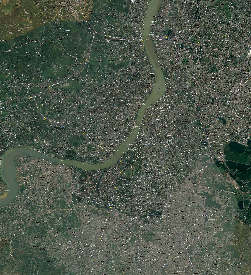
Figure 1: Scene-1, Bing Hybrid Map

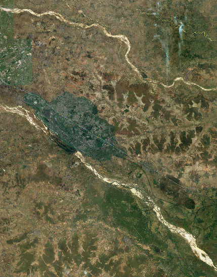
Figure 2: Scene-2, Bing Hybrid Map

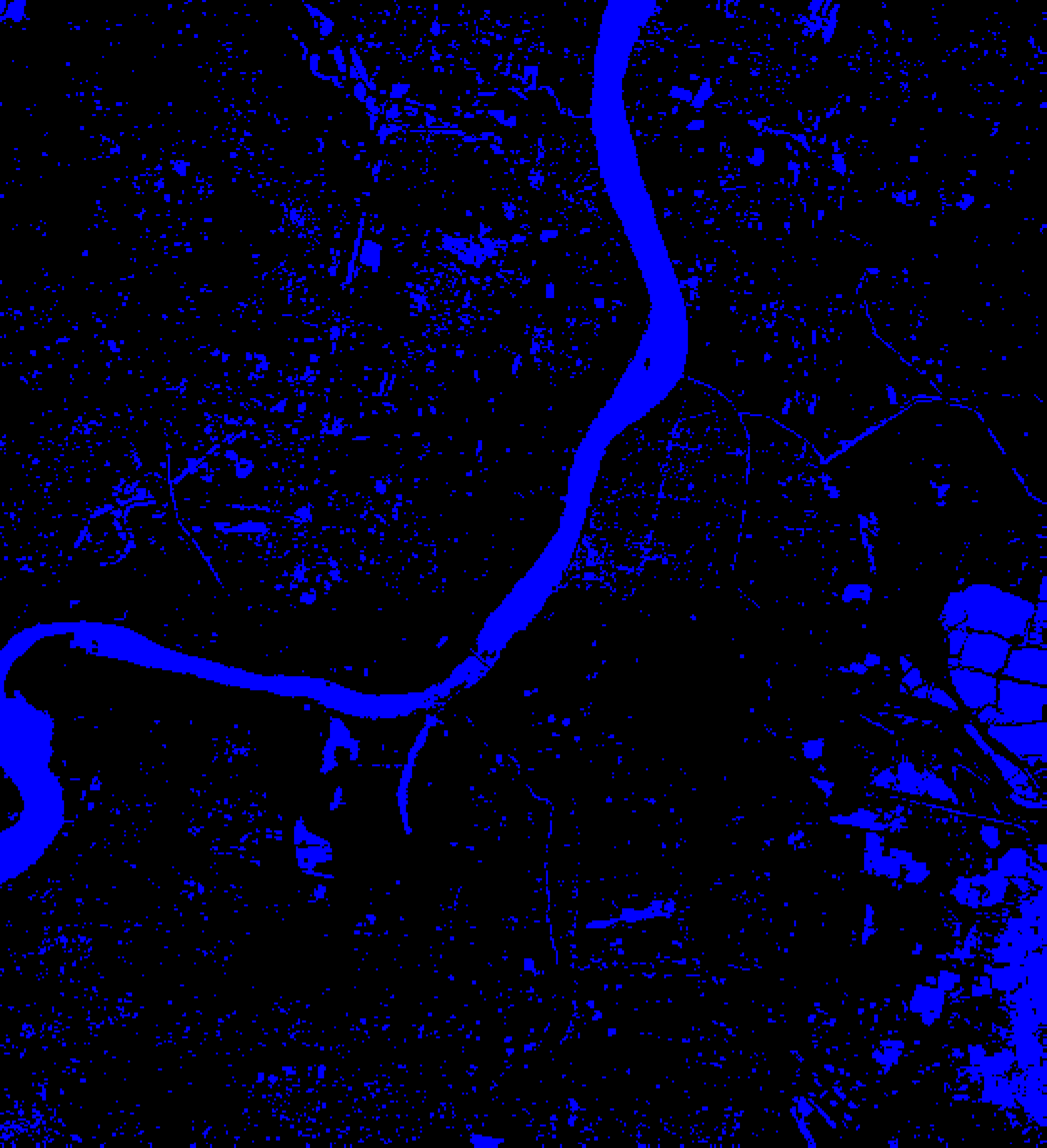
(a) water body, Scene-1 (WBS1)

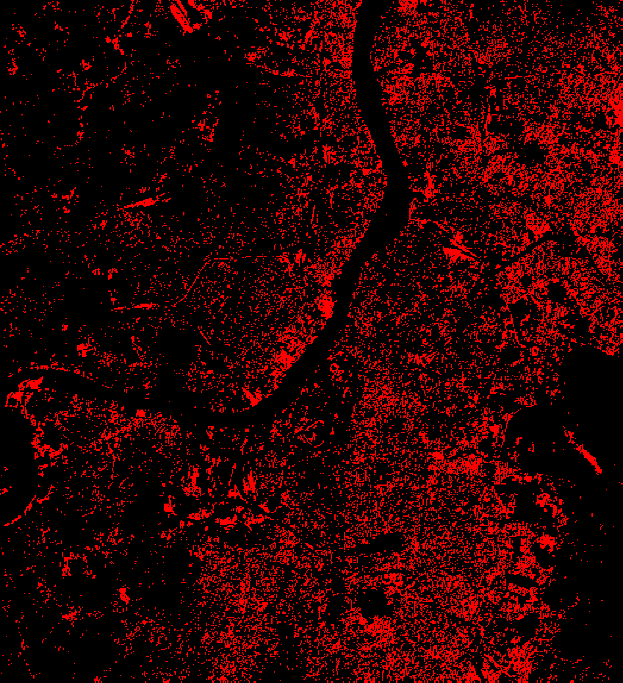
(b) built-up1, Scene-1 (B1S1)

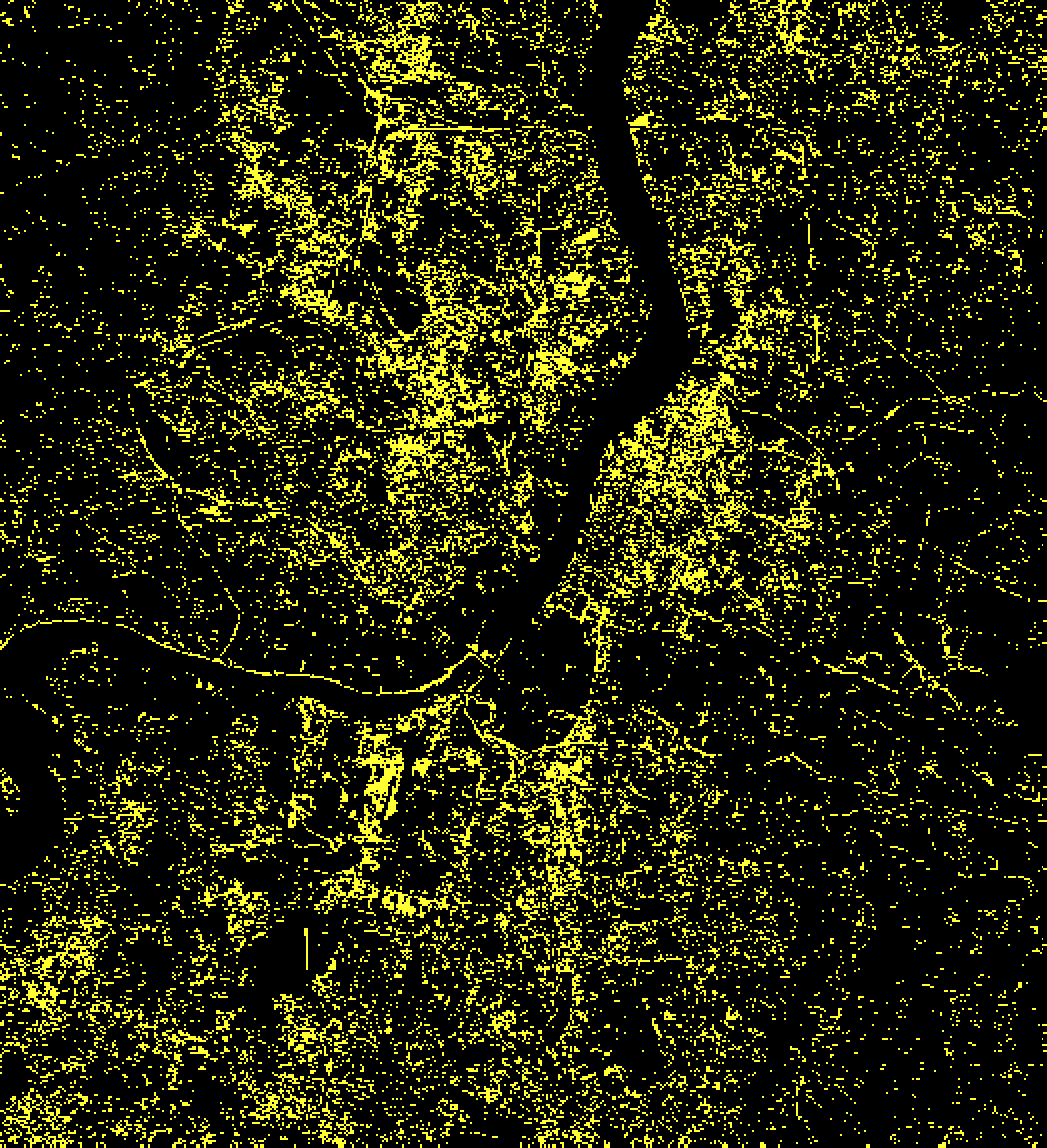
(c) built-up2, Scene-1 (B2S1)

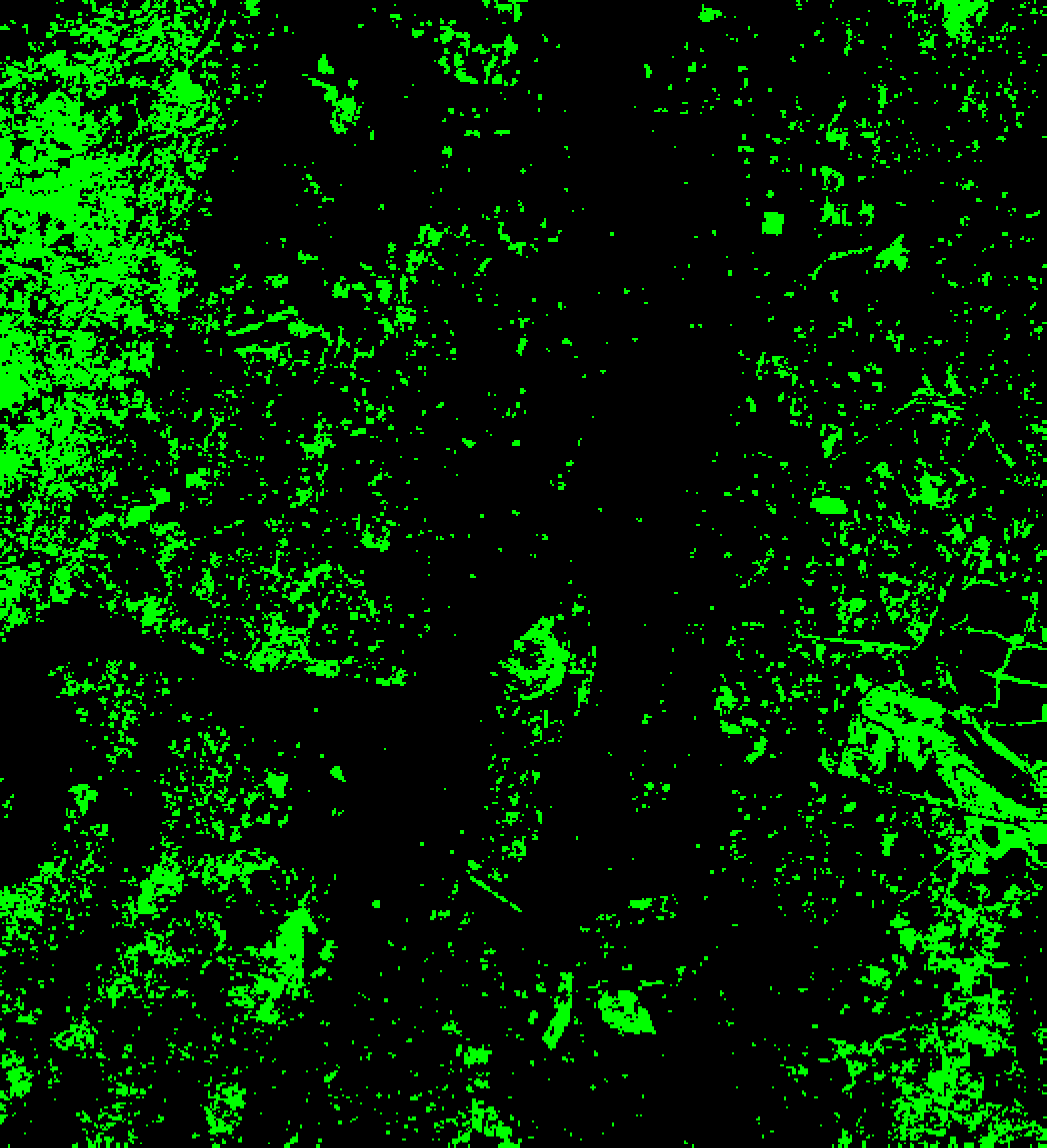
(d) vegetation, Scene-1 (V1S1)

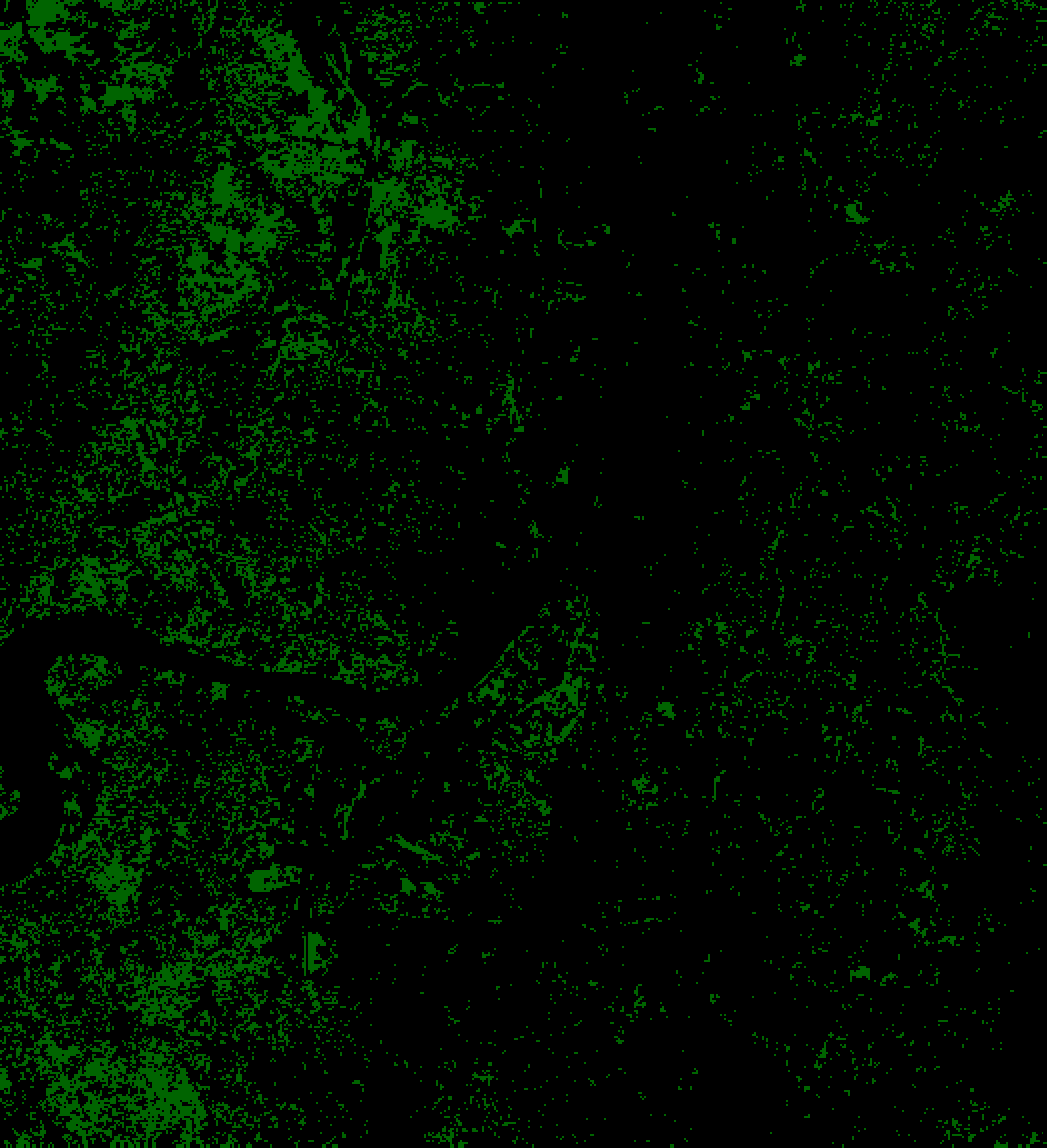
(e) vegetation, Scene-1 (V2S1)

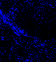
(f) waterbody, Scene-2 (cWBS2)

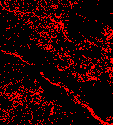
(g) wet-land, Scene-2 (cWLS2)

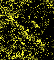
(h) vegetation, Scene-2 (cV1S2)

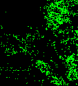
(i) vegetation, Scene-2 (cV2S2)

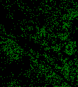
(j) vegetation, Scene-2 (cV3S2)

Figure 3: First and second rows show segmentation results of scene-1 and scene-2 respectively. The result set is generated using model-1.

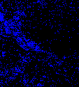
(a) water body, Scene-2 (WBS2)

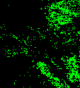
(b) vegetation, Scene-2 (V1S2)

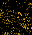
(c) Vegetation, Scene-2 (V2S2)

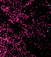
(d) Vegetation, Scene-2 (V3S2)

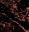
(e) Wetland, Scene-2 (WLS2)

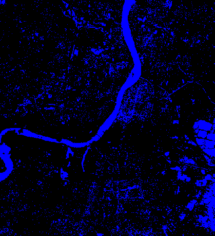
(f) water-body, Scene-1 (cWBS1)

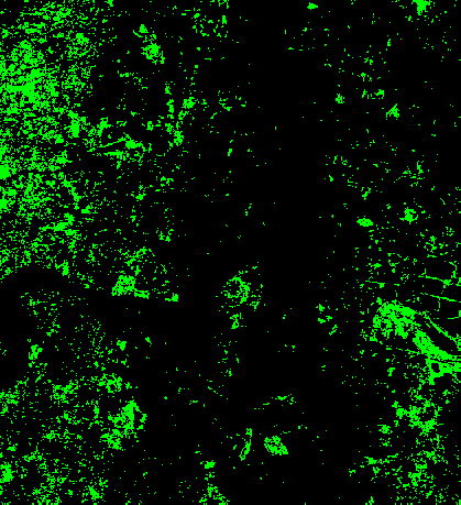
(g) Vegetation, Scene-1 (cV1S1)

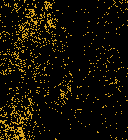
(h) vegetation, Scene-1 (cV2S1)

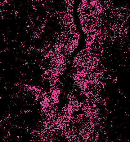
(i) built-up, Scene-1 (cB1S1)

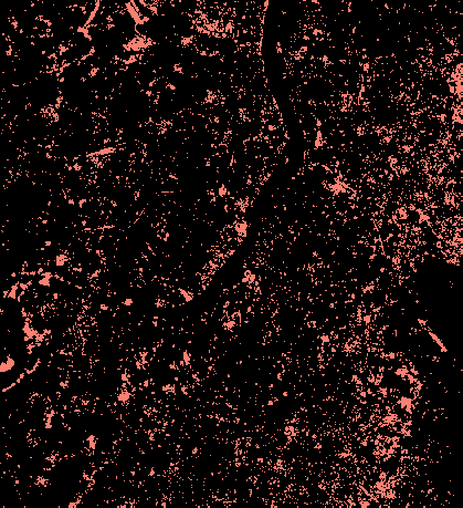
(j) built-up, Scene-1 (cB2S1)

Figure 4: First and second rows show segmentation results of scene-2 and scene-1 respectively. The result set is generated using model-2.

5 Conclusion

In this paper, we have proposed an approach to transform supervised CNN classifier architecture into an unsupervised clustering model. We address “structuredness” and “diversity” of the dataset to migrate from supervised to unsupervised paradigm. Our model jointly learns discriminative embedding subspace and cluster labels. The major strength of this approach is : scalability and re-usability. Experimental results show that RECAL performs competitively for real-world clustering task. However, it learns representation better compared to the existing approaches for non-face image datasets. We have shown segmentation as one of the application by our proposed method in remote sensing domain. To achieve this, we split the original image into small patches and get label for each of them. Then, they are combined to get the segmentation of the whole image. We qualitatively observe that this model is able to detect vegetation, water-body, wet-land, built-up area separately. We also provide the power of transferring learned representation across separate scenes in this work. However, built-up area has confusion with wetland and vegetation in cross-dataset segmentation task. It is probably due to the similar characteristics among these classes which is an innate problem in the underlying dataset. We also observe that training of the proposed network is fast. It took about roughly 30 hours to process more than 2 million patches in our experiments in GeForce GTX 1080 Ti GPU. This strongly indicates the property of scalability for our model.

References

- [1] A. Alqahtani, X. Xie, J. Deng, and M. W. Jones. A deep convolutional auto-encoder with embedded clustering. In 2018 25th IEEE International Conference on Image Processing (ICIP), pages 4058–4062, 2018.
- [2] D. Cai and X. Chen. Large scale spectral clustering via landmark-based sparse representation. IEEE Transactions on Cybernetics, 45:1669–1680, 2015.
- [3] K. G. Dizaji, A. Herandi, and H. Huang. Deep clustering via joint convolutional autoencoder embedding and relative entropy minimization. 2017 IEEE International Conference on Computer Vision (ICCV), pages 5747–5756, 2017.
- [4] X. Glorot and Y. Bengio. Understanding the difficulty of training deep feedforward neural networks. In Proceedings of the Thirteenth International Conference on Artificial Intelligence and Statistics, volume 9 of Proceedings of Machine Learning Research, pages 249–256, 2010.
- [5] D. B. Graham and N. M. Allinson. Characterising Virtual Eigensignatures for General Purpose Face Recognition, pages 446–456. 1998.
- [6] K. He, X. Zhang, S. Ren, and J. Sun. Deep residual learning for image recognition. CoRR, abs/1512.03385, 2015.
- [7] Y. Horibe. Entropy and correlation. IEEE Transactions on Systems, Man, and Cybernetics, SMC-15(5):641–642, 1985.
- [8] C. Hsu and C. Lin. Cnn-based joint clustering and representation learning with feature drift compensation for large-scale image data. IEEE Transactions on Multimedia, 20(2):421–429, 2018.
- [9] G. Huang, Z. Liu, and K. Q. Weinberger. Densely connected convolutional networks. CoRR, abs/1608.06993, 2016.
- [10] A. Krizhevsky, I. Sutskever, and G. E. Hinton. Imagenet classification with deep convolutional neural networks. In Proceedings of the 25th International Conference on Neural Information Processing Systems - Volume 1, NIPS’12, pages 1097–1105, 2012.
- [11] Y. Lecun, L. Bottou, Y. Bengio, and P. Haffner. Gradient-based learning applied to document recognition. Proceedings of the IEEE, 86(11):2278–2324, 1998.
- [12] S. A. Nene, S. K. Nayar, and H. Murase. Columbia object image library (coil-20. Technical report, 1996.
- [13] Y. Qin, X. Xiao, J. Dong, B. Chen, F. Liu, G. Zhang, Y. Zhang, J. Wang, and X. Wu. Quantifying annual changes in built-up area in complex urban-rural landscapes from analyses of palsar and landsat images. ISPRS Journal of Photogrammetry and Remote Sensing, 124:89 – 105, 2017.
- [14] J. Shi and J. Malik. Normalized cuts and image segmentation. IEEE Transactions on Pattern Analysis and Machine Intelligence, 22(8):888–905, 2000.
- [15] T. Sim, S. Baker, and M. Bsat. The cmu pose, illumination, and expression (pie) database. In Proceedings of the Fifth IEEE International Conference on Automatic Face and Gesture Recognition, FGR ’02, pages 53–, 2002.
- [16] K. Simonyan and A. Zisserman. Very deep convolutional networks for large-scale image recognition. CoRR, abs/1409.1556, 2014.
- [17] Y. Tan, F. Ren, and S. Xiong. Automatic extraction of built-up area based on deep convolution neural network. In 2017 IEEE International Geoscience and Remote Sensing Symposium (IGARSS), pages 3333–3336, 2017.
- [18] Y. Tan, S. Xiong, and Y. Li. Automatic extraction of built-up areas from panchromatic and multispectral remote sensing images using double-stream deep convolutional neural networks. IEEE Journal of Selected Topics in Applied Earth Observations and Remote Sensing, 11(11):3988–4004, 2018.
- [19] G. Trigeorgis, K. Bousmalis, S. Zafeiriou, and B. W. Schuller. A deep semi-nmf model for learning hidden representations. In Proceedings of the 31st International Conference on International Conference on Machine Learning - Volume 32, ICML’14, pages II–1692–II–1700. JMLR.org, 2014.
- [20] Z. Wang, S. Chang, J. Zhou, and T. S. Huang. Learning A task-specific deep architecture for clustering. CoRR, abs/1509.00151, 2015.
- [21] L. Wolf, T. Hassner, and I. Maoz. Face recognition in unconstrained videos with matched background similarity. In Proceedings of the 2011 IEEE Conference on Computer Vision and Pattern Recognition, CVPR ’11, pages 529–534, 2011.
- [22] J. Xie, R. B. Girshick, and A. Farhadi. Unsupervised deep embedding for clustering analysis. CoRR, abs/1511.06335, 2015.
- [23] J. Yang, D. Parikh, and D. Batra. Joint unsupervised learning of deep representations and image clusters. In 2016 IEEE Conference on Computer Vision and Pattern Recognition (CVPR), pages 5147–5156, 2016.
- [24] Y. Yang, D. Xu, F. Nie, S. Yan, and Y. Zhuang. Image clustering using local discriminant models and global integration. IEEE Transactions on Image Processing, 19(10):2761–2773, 2010.
- [25] L. Zelnik-Manor and P. Perona. Self-tuning spectral clustering. In Proceedings of the 17th International Conference on Neural Information Processing Systems, NIPS’04, pages 1601–1608, 2004.
- [26] W. Zhang, X. Wang, D. Zhao, and X. Tang. Graph degree linkage: Agglomerative clustering on a directed graph. CoRR, abs/1208.5092, 2012.
- [27] W. Zhang, D. Zhao, and X. Wang. Agglomerative clustering via maximum incremental path integral. Pattern Recognition, 46(11):3056 – 3065, 2013.