An all order exact result for the anomalous dimension of the scalar primary in Chern Simons Vector Models

Abstract

We present a conjecture for the leading $1/N$ anomalous dimension of the scalar primary operator in $U(N)_{k}$ Chern-Simons theories coupled to a single fundamental field, to all orders in the t’Hooft coupling $\lambda=\frac{N}{k}$. Following this we compute the anomalous dimension of the scalar in a Regular Bosonic theory perturbatively at two-loop order and demonstrate that matches exactly with the result predicted by our conjecture. We also show that our proposed expression for the anomalous dimension is consistent with all other existing two-loop perturbative results, which constrain its form at both weak and strong coupling thanks to the bosonization duality. Furthermore, our conjecture passes a novel non-trivial all loop test which provides a strong evidence for its consistency.

I Introduction

$U(N)_{k}$ Chern-Simons theories coupled to a single fundamental field are an important class of conformal field theories that are solvable in the large $N$ limit Giombi:2011kc ; Aharony:2011jz . As emphasized in MZ ; Aharony:2012nh ; Skvortsov:2018uru four such theories exist depending on the choice of fundamental matter, which can be divided into two classes: quasi-fermionic and quasi-bosonic. The quasi-fermionic class includes the theory with one species of fundamental fermions as matter and the theory with critical (Wilson-Fisher) bosons as matter. Both these theories are believed to be related by a strong-weak coupling duality MZ ; Aharony:2012nh ; Skvortsov:2018uru ; GurAri:2012is ; Aharony:2012ns ; Gur-Ari:2015pca ; Bedhotiya:2015uga ; Minwalla:2015sca ; Aharony:2015mjs . The quasi-bosonic class includes the theory with matter as (non-critical) bosons and the theory with critical (Gross-Neveu) fermions as matter. Again, both these theories are related by strong-weak duality, discussed extensively in Aharony:2018pjn . See also, e.g., Yokoyama:2016sbx ; Seiberg:2016gmd ; Murugan:2016zal ; Kachru:2016rui ; Radicevic:2016wqn ; Hsin:2016blu ; Jain:2013py ; Jain:2013gza ; Jain:2014nza for additional tests and discussion of the bosonization duality.

An important feature of these theories is that they contain a very sparse spectrum of single-trace primary operators. There is exactly one single-trace primary operator for each spin $s$, which we denote as $j_{s}$. When ’t Hooft coupling $\lambda=0$, these currents are exactly conserved, and therefore have scaling dimensions given by the unitarity bound $\Delta_{s}=s+1$ for nonzero $s$. As argued in Giombi:2011kc ; Aharony:2011jz , a simple argument based on conformal representation theory implies that the scaling dimensions of these currents are protected in the large $N$ limit, even when $\lambda\neq 0$. The leading corrections to the scaling dimensions are proportional to $1/N$: $\Delta_{s}=(s+1)+\gamma_{s}(\lambda)+O(\frac{1}{N^{2}})$ where $\gamma_{s}(\lambda)$ corresponds to the anomalous dimension of spins-$s$ primary operator at order $1/N$. For operators with spin $s\neq 0$, the scaling dimensions can be determined from planar three-point functions using the slightly broken higher-spin symmetry MZ of the theory Giombi:2016zwa .

The results and methods of Giombi:2016zwa rely on slightly-broken higher-spin symmetry Giombi:2016hkj ; Nii:2016lpa ; Skvortsov:2015pea , and are valid only for $s\neq 0$. Although it is possible to analytically continue the formulas derived in Giombi:2016zwa , this gives us a result that is inconsistent with perturbative computations (which are possible at both weak and strong coupling thanks to the bosonization duality). Hence the leading $1/N$ correction to the anomalous dimension of the scalar primary $j_{0}$ remains unknown at present. This quantity is interesting for a variety of reasons. As argued in Aharony:2018pjn , it plays an important role in determining the fixed point for the $\phi^{6}$ coupling in the quasi-bosonic family of theories at $1/N$.

Quite interestingly, in condensed matter physics, the scaling dimension of $j_{0}$ is extremely significant as it determines an experimentally-measurable critical exponent for certain quantum Hall phase transitions WenWu ; Mott ; Hui:2017pwe ; Hui:2017cyz . However, for comparison with experiments one would require finite and small $N$. In this context, the anomalous dimension of the scalar primary is one of the simplest physical observables for our theory, and it is rather striking that it remains unknown.

In principle, an exact Feynman diagram calculation could be performed to calculate the anomalous dimension of $j_{0}$ to all orders in $\lambda$ using the light-cone gauge, (as discussed in Gurucharan:2014cva ) but this is not a possibility at present for what appear to be insurmountable technical reasons. In particular, one of the crucial ingredients, the exact ladder diagram Aharony:2012nh ; Bedhotiya:2015uga , is not known off-shell.

Here, motivated by the results Giombi:2016zwa for $\gamma_{s}$, and perturbative calculations, including a new a calculation of the two-loop anomalous dimension of the scalar primary in the theory coupled to fundamental bosons, we conjecture a simple all-orders expression for the anomalous dimension $s=0$. We will show that this conjecture passes several non-trivial consistency checks.

The article is organized as follows. In section II we briefly discuss the parameters in the quasi-bosonic and quasi fermionic theory and setup our notations for those parameters. In section III we perform a perturbative computation of the anomalous dimension for the scalar in the regular bosonic theory and also describe the result for the critical fermionic theory in the literature. Following this, in section IV we describe the results for the anomalous dimension in quasi-fermionic theories. Following this, in section V we briefly review a result obtained in Aharony:2018pjn which serves as an all loop test for our proposal. In section VI we demonstrate that the naive analytic continuation of the spins-$s$ operator to $s=0$ fails to reproduced the correct anomalous dimension for all the theories. Subsequently in section VII we propose our conjecture for the anomalous dimension of the scalar operators in both quasi-fermionic and quasi-bosonic and demonstrate that our conjecture reproduces all known perturbative results and also passes a non-trivial all loop test. In Appendix we will argue that our conjecture can also be thought of as a two-sided Padé approximation, which makes use of perturbative data at both weak and strong coupling, in the spirit of S-dualty improved perturbation theory Sen:2013oza . Of course, this is only possible because of the bosonization duality.

II Parameters and Theories

Let us carefully review the theories under study and their relations via RG flow and bosonization duality.

The quasi-bosonic family of theories flows to the quasi-fermionic family of theories under RG flow. In MZ , the quasi-bosonic family is described by three parameters $\tilde{\lambda}_{QB}$, $\tilde{N}_{QB}$ and $\tilde{\lambda}_{6,QB}$; and the quasi-fermionic family is described by two parameters $\tilde{\lambda}_{QF}$ and $\tilde{N}_{QF}$. The parameter $\tilde{N}$ is defined via the two-point function of the stress-energy tensor, and is a measure of the number of degrees of freedom of each theory – we will only be interested in the large $\tilde{N}$ limit and the first non-trivial $1/\tilde{N}$ corrections. In this limit, the spectrum is independent of the parameter $\tilde{\lambda}_{6,QB}$ so we will ignore it in the discussion that follows.

The celebrated bosonization duality states that each family of theories has two very-different-looking descriptions. The quasi-bosonic family can be described as a theory of $N_{b}$ complex bosons transforming in the fundamental representation of $U(N_{b})$, coupled to a level-$\kappa_{b}$ Chern-Simons gauge field. It can also be described as a theory of $N_{f}$ Dirac “critical” fermions, in the fundamental representation of $U(N_{f})$ coupled to a level $\kappa_{f}$ Chern-Simons gauge field. The quasi-fermionic family can be described as a theory of $N_{b}$ critical complex bosons transforming in the fundamental representation of $U(N_{b})$, coupled to a level-$\kappa_{b}$ Chern-Simons gauge field. It can also be described as a theory of $N_{f}$ Dirac fermions, in the fundamental representation of $U(N_{f})$ coupled to a level $\kappa_{f}$ Chern-Simons gauge field.

This duality is well-tested in the large $N_{b/f}$ limit, with $\lambda_{b/f}\equiv\frac{N_{b/f}}{k_{b/f}}$ held fixed. In this limit we have the following relation between the parameters:

$$\tilde{N}_{QB} = 2N_{b}\frac{\sin(\pi\lambda_{b})}{\pi\lambda_{b}}=2N_{f}\frac{\sin(\pi\lambda_{f})}{\pi\lambda_{f}}$$

$$\tilde{N}_{QF} = 2N_{b}\frac{\sin(\pi\lambda_{b})}{\pi\lambda_{b}}=2N_{f}\frac{\sin(\pi\lambda_{f})}{\pi\lambda_{f}}$$ (1)

$$\tilde{\lambda}_{QB} = \tan\left(\frac{\pi\lambda_{b}}{2}\right)=\cot\left(\frac{\pi\lambda_{f}}{2}\right)$$

$$\tilde{\lambda}_{QF} = \cot\left(\frac{\pi\lambda_{b}}{2}\right)=\tan\left(\frac{\pi\lambda_{f}}{2}\right)$$

Because $N_{b/f}$ and $\kappa_{b/f}$ are integers (or half-integers), the parameters $\lambda_{b/f}$ and $N_{b/f}$ do not run under RG flow from quasi-bosonic theory to quasi-fermionic theory. Under RG flow, the quasi-bosonic theory defined by $\tilde{\lambda}_{QB}$ and $\tilde{N}_{QB}$ flows to the quasi-fermionic theory described by:

$$\tilde{\lambda}_{QF} = \frac{1}{\tilde{\lambda}_{QB}}$$ (2)

$$\tilde{N}_{QF} = \tilde{N}_{QB}.$$ (3)

We henceforth use $\tilde{N}$ without any subscript.

Let us denote the scaling dimension of the scalar primary $j_{0}$ in the quasi-bosonic theory as $\Delta_{0}$, and the scaling dimension of $\tilde{j}_{0}$ in the QF theory as $\tilde{\Delta}_{0}$. We define the anomalous dimension as:

$$\Delta_{0}=1+\gamma_{0},~{}~{}~{}\tilde{\Delta}_{0}=2+\tilde{\gamma}_{0}$$ (4)

III Quasi-Bosonic Theories

III.1 Perturbative Computations in the Regular Bosonic Theory

In this section, we begin by computing the anomalous dimension of $j_{0}=\bar{\phi}\phi$ in the regular bosonic theory, i.e., $SU(N)_{k}$ Chern Simons theory coupled to a single complex scalar field, to two loops. (The leading $1/N$ correction to the anomalous dimension is the same whether one considers the $U(N)$ or $SU(N)$ theories, although subleading corrections may differ.) This will serve as a non-trivial check for our conjecture. Our computation closely follows the calculation of the anomalous dimension of $j_{0}$ in the $O(N)$ theory carried out in Aharony:2011jz . All our calculations in this appendix are in the bosonic theory, so we drop the subscript $b$ in what follows.

We also refer to related perturbative computations in Chern-Simons theory which appear in Avdeev:1991za ; Ivanov:1991fn ; Chen:1992ee ; Banerjee:2013nca . To this end, we calculate the anomalous dimension of the operator $j_{0}$ at two loops. The diagrams which we need to evaluate are given in figure 1,2,3. Our conventions, Feynman rules and gauge choices are provided in the appendix Acknowledgements

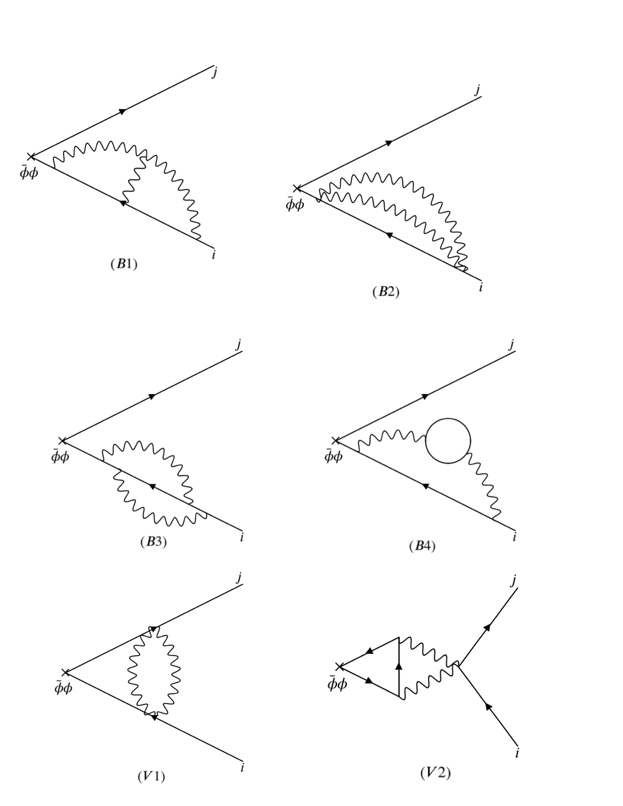
Figure 1: Diagrams ($B1$)-($B4$) depict loop corrections to the propagator. Diagrams (V1) and (V2) are loop corrections to the vertex.

The logarithmic divergences arising due to the loop correction of the propagators depicted in the diagrams ($B1$)-($B4$) of the figure 1 are given by

$$(B1) = \frac{2}{3k^{2}}C_{2}C_{3}~{}\log[\Lambda]=\frac{1-N^{2}}{3k^{2}}~{}\log[\Lambda]$$ (5)

$$(B2) = \frac{2}{3k^{2}}(C_{3}^{2}+\frac{C_{2}C_{3}}{4})~{}\log[\Lambda]=\frac{N^{4}-3N^{2}+2}{12k^{2}N^{2}}\log[\Lambda]$$

$$(B3) = \frac{8}{3k^{2}}(C_{3}^{2}+\frac{C_{2}C_{3}}{2})\log[\Lambda]=\frac{2}{3k^{2}}(\frac{1}{N^{2}}-1)\log[\Lambda]$$

$$(B4) = \frac{4}{3k^{2}}C_{1}C_{3}\log[\Lambda]=\frac{1}{3k^{2}}\left(N-\frac{1}{N}\right)\log[\Lambda]$$

The logarithmic divergences arising from the corrections to the vertex depicted in figure 1 are given by

$$(V1) = \frac{4}{k^{2}}(C_{3}^{2}+\frac{C_{2}C_{3}}{4})~{}\log[\Lambda]=\frac{N^{4}-3N^{2}+2}{2~{}k^{2}N^{2}}\log[\Lambda]$$

$$(V2) = \frac{8}{k^{2}}C_{1}C_{3}~{}\log[\Lambda]=\frac{2}{k^{2}}\left(N-\frac{1}{N}\right)\log[\Lambda].$$ (6)

Following Gurucharan:2014cva , we use these results, to compute the $\mathcal{O}(\frac{1}{N})$ logarithmic divergence of the two-point function $\langle j_{0}j_{0}\rangle$ to be:

$$2(B1+B2+B3+B4)+V1+V2=\frac{8}{3}\frac{\lambda^{2}}{N}\log[\Lambda]+O(\frac{1}{N^{2}}),$$ (7)

where we have used re-expressed the result in terms of $\lambda\equiv\frac{N}{k}$. Note that the $U(N)$ result is just the large-$N$ limit of the $SU(N)$ result.

Note that the loop corrections to the propagator should be taken on each of the two legs of the vertex diagrams ($B1$)-($B4$) depicted in figure 1 and hence they contribute twice to the two-point function.

Now we briefly describe how to obtain the anomalous dimension of operator $j_{0}$ from two point function of the same operator.The two-point correlation function of the scalars in a $d$-dimensional CFT in momentum space is given by

$$\langle j_{0}(p)j_{0}(0)\rangle=\frac{c_{1}}{p^{2\Delta-d}}.$$ (8)

The scaling dimension $\Delta$ can be expressed in $\frac{1}{N}$ expansion as

$$\Delta=\Delta_{0}+\gamma_{0}+O(\frac{1}{N^{2}})$$ (9)

where $\Delta_{0}$ is classical scaling dimension, $\gamma_{0}$ is anomalous dimension to order $\frac{1}{N}$. Plugging (9) in (8) and expanding to leading order around $\gamma_{0}=0$, we obtain

$$\langle j_{0}(p)j_{0}(0)\rangle = \frac{1}{p^{2\Delta_{0}-d}}(1-2\gamma_{0}\log{p})]$$ (10)

Hence the anomalous dimension is given by $-1/2$ times the logarithmic divergence we obtained earlier. Keeping corrections in the anomalous dimension upto $\mathcal{O}[\frac{1}{N}]$, this leads us to the following expression for the anomalous dimension at $\mathcal{O}[\lambda_{b}^{2}]$

$$\gamma_{0}=\frac{1}{N_{b}}\left(-\frac{4}{3}\lambda_{b}^{2}+O(\lambda_{b}^{4})\right).$$ (11)

In a subsequent section, we will demonstrate that the anomalous dimension in Eq.(11) matches exactly with the perturbative expansion of our conjectured expression in (52).

III.2 UV Finite diagrams

Apart from the diagrams depicted in fig.1 there are other two-loop diagrams which do not contribute to the anomalous dimension at order $1/N$. They are depicted in Figure 2.

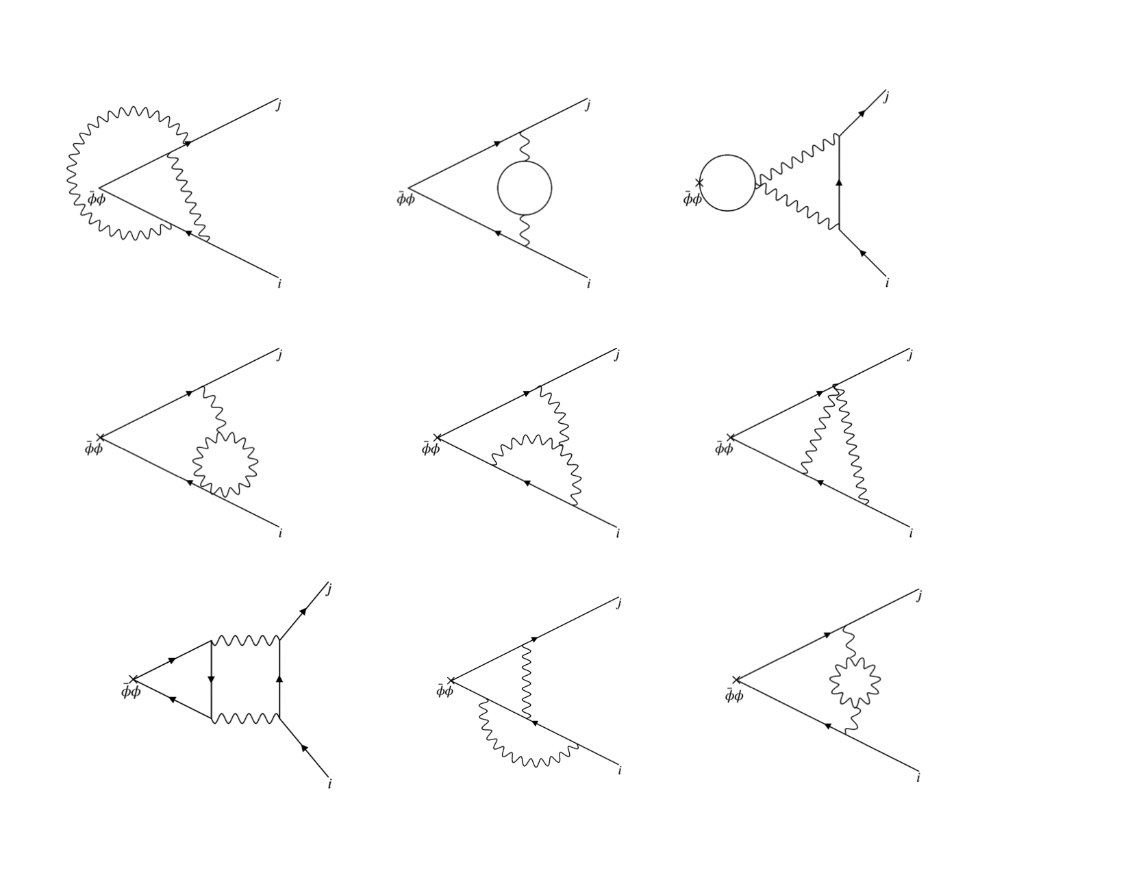
Figure 2: All the diagrams appearing in this figure do not contribute to the anomalous dimension at $1/N$.

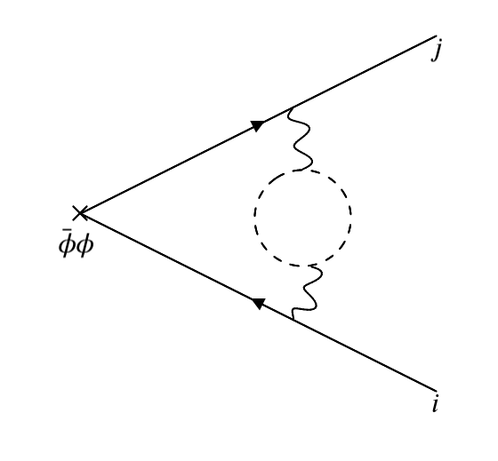
Figure 3: Diagram with a ghost loop which cancels the last diagram in Fig.2.

III.3 Critical Fermionic Theory

Figure 4: The feynman diagrams that contribute in the critical fermionic theory Giombi:2016zwa .

The order $\lambda_{f}^{2}$ correction anomalous dimension in the critical fermionic theory was determined through a direct Feynman diagram computation in Muta:1976js ; Giombi:2016zwa to be

$$\gamma_{0}=\frac{1}{N_{f}}\left(-\frac{16}{3\pi^{2}}+\frac{4}{9}\lambda_{f}^{2}+O(\lambda_{f}^{4})\right).$$ (12)

The diagrams that contribute to the anomalous dimension at order $\lambda_{f}^{2}$ in the critical fermionic theory are depicted in Fig. 4.

IV Quasi-Fermionic Theory

The leading order $1/N$ anomalous dimension for the critical bosonic theory appears in Lang:1992zw (see also Skvortsov:2015pea ; Giombi:2016hkj ). We carried out a calculation of the order-$\lambda_{b}^{2}$ correction to this quantity to obtain:

$$\tilde{\gamma}_{0}=\frac{1}{N_{b}}\left(-\frac{16}{3\pi^{2}}+\frac{4}{9}\lambda_{b}^{2}+O(\lambda_{b}^{4})\right).$$ (13)

To order $\lambda_{f}^{2}$, the anomalous dimension of $\tilde{j}_{0}$ in the regular fermionic theory was computed through a direct Feynman diagram technique in Gurucharan:2014cva ; Giombi:2016zwa

$$\tilde{\gamma}_{0}=\frac{1}{N_{f}}\left(-\frac{4}{3}\lambda_{f}^{2}+O(\lambda_{f}^{4})\right).$$ (14)

Figure 5: The feynman diagrams that contribute in the Regular fermionic theory Giombi:2016zwa .

The diagrams that contribute to the anomalous dimension at order $\lambda_{f}^{2}$ in the regular fermionic theory are depicted in Fig. 5.

V All loop test

Here we briefly review the computation in Aharony:2018pjn where the authors determine the $1/N$ correction to the sum of the anomalous dimension in the quasi-bosonic and the quasi-fermionic theories which will later serve as a highly non-trivial all loop consistency check for our conjecture.

To this end, the authors begin by the action of critical boson $(S_{CB}(\phi,\sigma))$ and the regular fermionic theories are given by

$$S_{CB}\left(\phi,\sigma_{B}\right) =\int d^{3}x[i\varepsilon^{\mu\nu\rho}\frac{\kappa_{B}}{4\pi}\operatorname{Tr}\left(A_{\mu}\partial_{\nu}A_{\rho}-\frac{2i}{3}A_{\mu}A_{\nu}A_{\rho}\right)+i\varepsilon^{\mu\nu\rho}\frac{N_{B}\kappa_{B}^{\prime}}{4\pi}B_{\mu}\partial_{\nu}B_{\rho}$$

$$~{}~{}~{}~{}~{}~{}~{}~{}~{}~{}~{}~{}~{}~{}~{}\left.+D_{\mu}\bar{\phi}D^{\mu}\phi+\sigma_{B}\bar{\phi}\phi\right]$$ (15)

$$S_{RF}(\psi) =\int d^{3}x\left[i\varepsilon^{\mu\nu\rho}\frac{\kappa_{F}}{4\pi}\operatorname{Tr}\left(A_{\mu}\partial_{\nu}A_{\rho}-\frac{2i}{3}A_{\mu}A_{\nu}A_{\rho}\right)+\bar{\psi}\gamma_{\mu}D^{\mu}\psi\right]$$ (16)

where $k_{B}$ corresponds to the level of $SU(N_{B})$ gauge field denoted above as $A_{\mu}$ and $k^{\prime}_{B}$ corresponds to the level of a $U(N_{B})$ gauge field $B_{\mu}$. These two combine to form $U\left(N_{B}\right)=\left(SU\left(N_{B}\right)\times U(1)\right)/Z_{N_{B}}$.

The action for the regular bosonic and critical fermionic theories may be obtained as a relevant deformation of the critical bosonic and regular fermionic theories as follows

$$S_{RB}(\phi,\sigma,\zeta) =S_{CB}(\phi,\sigma)-\int\tilde{J}_{0}(x)\zeta(x)$$

$$~{}~{}~{}~{}+\frac{(2\pi)^{2}}{\kappa_{B}^{2}}\left(x_{6}^{B}+1\right)\int\zeta^{3}(x)$$ (17)

$$S_{CF}(\psi,\zeta) =S_{RF}(\psi)-\int J_{0}^{F}(x)\zeta(x)r$$ (18)

$$~{}~{}~{}~{}+\frac{(2\pi)^{2}}{\tilde{\kappa}_{F}^{2}}x_{6}^{F}\int\zeta^{3}(x)$$ (19)

where the subscripts $RB,CB,RF$ and $CF$ denote the regular bosonic theory, critical bosonic theory, regular fermionic theory and critical fermionic theory respectively. Note that $\tilde{J_{0}}$ and $J_{0}^{F}$ are operators of scaling dimension $2$ which act as sources for new dynamical field $\zeta$. $x_{6}^{B}$ and $x_{6}^{F}$ are parameters.

The effective action for the critical fermionic and the regular bosonic theories is obtained by integrating out the appropriate fields as

$$\int D\phi D\sigma e^{-S_{RB}(\phi,\sigma,\zeta)} =e^{-S_{RB}^{eff}(\zeta)}$$ (20)

$$\int D\psi e^{-S_{CF}(\psi,\zeta)} =e^{-S_{CF}^{\epsilon ff}(\zeta)}$$ (21)

The authors observe that for $x_{6}^{B}=x_{6}^{F}$ the theories in eq.(17) and eq.(19) are identical and the conjectured duality leads to

$$S_{RB}^{eff}\left(\zeta;\kappa_{B},\lambda_{B}\right)=S_{CF}^{eff}\left(\zeta;-\kappa_{B},\lambda_{B}-\operatorname{sgn}\left(\lambda_{B}\right)\right)$$ (22)

This in turn implies that 1PI quantum effective action for both the theories are also identical as they are computed through the path integral of the above effective actions

$$S_{RB}^{1PI}(\zeta)=S_{CF}^{1PI}(\zeta)$$ (23)

In order to extract the difference between the anomalous dimensions of the two theories, the authors first evaluate the UV cut-off ($\Lambda$) dependent quintic and quartic terms in effective action $S_{RB}^{eff}(\zeta)$ at leading order in $1/N$ to be

$$S_{RB}^{eff} =\frac{g_{2}}{2\kappa_{B}}\int\frac{d^{3}q}{(2\pi)^{3}}|q|\left(\frac{|q|}{\Lambda}\right)^{\frac{2\delta_{B}\left(\lambda_{B}\right)}{\kappa_{B}}}\zeta(q)\zeta(-q)$$

$$+\frac{g_{3}}{6\kappa_{B}^{2}}\int\frac{d^{3}q_{1}}{(2\pi)^{3}}\frac{d^{3}q_{2}}{(2\pi)^{3}}\frac{d^{3}q_{3}}{(2\pi)^{3}}(2\pi)^{3}\delta\left(q_{1}+q_{3}\right)\zeta\left(q_{1}\right)\zeta\left(q_{2}\right)\zeta\left(q_{3}\right)$$

$$+\frac{\tilde{g}_{3}}{6\kappa_{B}^{2}}\int\frac{d^{3}q_{1}}{(2\pi)^{3}}\frac{d^{3}q_{2}}{(2\pi)^{3}}\frac{d^{3}q_{3}}{(2\pi)^{3}}(2\pi)^{3}\frac{\delta_{B}}{\kappa_{B}}\ln\left(\frac{\Lambda}{\left|q_{1}\right|+\left|q_{2}\right|+\left|q_{3}\right|}\right)\delta\left(q_{1}+q_{2}+q_{3}\right)\zeta\left(q_{1}\right)\zeta\left(q_{2}\right)\zeta\left(q_{3}\right)$$

$$-\frac{1}{24\kappa_{B}^{3}}\int\prod_{i=1}^{4}\frac{d^{3}q_{i}}{(2\pi)^{3}}(2\pi)^{3}\delta\left(q_{1}+q_{2}+q_{4}+q_{4}\right)\kappa_{B}^{3}\tilde{G}_{4}^{0}\left(q_{1},q_{2},q_{3},q_{4}\right)\zeta\left(q_{1}\right)\zeta\left(q_{2}\right)\zeta\left(q_{3}\right)\zeta\left(q_{4}\right)$$

$$-\frac{1}{5!\kappa_{B}^{4}}\int\prod_{i=1}^{5}\frac{d^{3}q_{i}}{(2\pi)^{3}}(2\pi)^{3}\delta\left(q_{1}+q_{2}+q_{3}+q_{4}+q_{5}\right)\kappa_{B}^{4}\tilde{G}_{5}^{0}\left(q_{1},q_{2},q_{3},q_{4},q_{5}\right)\zeta\left(q_{1}\right)\zeta\left(q_{2}\right)\zeta\left(q_{3}\right)\zeta\left(q_{4}\right)\zeta\left(q_{5}\right)$$ (24)

where $g_{2},g_{3}$ and $\tilde{g_{3}}$ are functions of $\lambda_{B}$ and $x_{6}^{B}$ (See Aharony:2018pjn for details). Following this the authors then compute the one loop correction to the above

$$S_{RB}^{1PI}(\zeta)-S_{RB}^{eff}(\zeta)=\frac{1}{2\kappa_{D}^{2}}\int\frac{d^{3}q}{(2\pi)^{3}}\delta\Gamma_{2}(q)\zeta(q)\zeta(-q)$$ (25)

where

$$\delta\Gamma_{2}(q)=-\frac{32}{3\pi\sin\pi\lambda_{B}}|q|\ln\left(\frac{\Lambda}{|q|}\right)$$ (26)

Hence the 1PI quantum effective action for the regular bosonic theory in the above equation is of the form

$$S_{RB}^{1PI}=\frac{g_{2}}{2\kappa_{B}}\int\frac{d^{3}q}{(2\pi)^{3}}|q|\left(\frac{|q|}{\Lambda}\right)^{\frac{2\delta^{\prime}_{\beta}\left(\lambda_{B}\right)}{\kappa_{B}}}\zeta(q)\zeta(-q)$$ (27)

Comparing eq.(24) and eq.(27) we obtain the difference between the anomalous dimension of the two theories to be

$$\delta_{B}^{\prime}-\delta_{B}=\frac{16}{3\pi\sin\pi\lambda_{B}}$$ (28)

These are related to the scaling dimension of the $\zeta$ and $\sigma$ operators $\Delta_{\zeta}=\Delta_{j_{0}}$ and $\Delta_{\sigma}=\Delta_{\tilde{j}_{0}}$ as

$$\Delta_{\zeta}=1-\frac{\delta_{B}^{\prime}}{\kappa_{B}}~{}~{}~{}~{}~{}~{}\Delta_{\sigma}=2+\frac{\delta_{B}}{\kappa_{B}}$$ (29)

Comparing the above equation and eq.(28) we obtain

$$\delta_{B}^{\prime}=-\gamma_{0}$$

$$\delta_{B}=\tilde{\gamma}_{0}.$$ (30)

Hence, eq.(28) and eq.(30) lead to the following relation between the anomalous dimension of the quasi-bosonic and quasi-fermionic theories

$$\tilde{\gamma}_{0}+\gamma_{0} =-\frac{16\lambda_{b}}{3\pi\sin\pi\lambda_{b}}\frac{1}{N_{b}}=-\frac{16\lambda_{f}}{3\pi\sin\pi\lambda_{f}}\frac{1}{N_{f}}$$

$$=-\frac{32}{3\pi^{2}}\frac{1}{\tilde{N}},$$ (31)

Note the above relation at order $\lambda^{2}$ becomes

$$\tilde{\gamma}_{0}+\gamma_{0}=-\frac{16}{3\pi^{2}}-\frac{8\lambda_{b}^{2}}{9}+O[\lambda_{b}^{4}]$$ (32)

Note that the above result is exaclty satisfied by the two loop perturbative expressions for the anomalous dimension of the regular and critical bosonic theories given by eq.(11) and eq.(13). Similarly its easy to check the above equation is satified by the result for the regular and critical fermionic theories in eq.(14) and eq.(12). In the subsequent sections we will demonstrate that our conjectured expression for the anomalous dimension satisfies (31) to all orders in $\lambda$. This will provide strong evidence for the consistency of our conjecture.

VI Towards an all loop result

The authors in Giombi:2016zwa utilized the non-conservation of the higher spin currents to demonstrate that $1/N$ higher-spin spectrum for the quasi-fermionic theory,to all orders in $\tilde{\lambda}_{QF}$ for the spinning operator $J_{s}$, is given by

$$\gamma^{QF}_{s}=\frac{1}{\tilde{N}}\left(a_{s}^{QF}\frac{\tilde{\lambda}_{QF}^{2}}{1+\tilde{\lambda}_{QF}^{2}}+b_{s}^{QF}\frac{\tilde{\lambda}_{QF}^{2}}{(1+\tilde{\lambda}_{QF}^{2})^{2}}\right)+O(\frac{1}{N^{2}}).$$ (33)

Here $\gamma^{QF}_{s}=\Delta_{s}-(s+1)$ is the anomalous dimension of the spin-$s$ primary. A similar expression holds for the quasi-bosonic theory.

The expressions for the spin-dependent constants turn out to be identical for both the quasi-bosonic and quasi-fermionic theories and is

$$a_{s} = \begin{cases}\frac{16}{3\pi^{2}}\frac{s-2}{2s-1}\,,&\text{for even $s$}\,,\\ \frac{32}{3\pi^{2}}\frac{s^{2}-1}{4s^{2}-1}\,,&\text{ for odd $s$}\,,\end{cases}$$ (34)

$$b_{s} = \begin{cases}\frac{2}{3\pi^{2}}\left(3\displaystyle\sum_{n=1}^{s}\frac{1}{n-\frac{1}{2}}+f(s)\right)\,,&\\ \text{for even $s$}\,,\\ \frac{2}{3\pi^{2}}\left(3\displaystyle\sum_{n=1}^{s}\frac{1}{n-\frac{1}{2}}+g(s)\right)\,,&\\ \text{ for odd $s$}\,.\end{cases}$$ (35)

$$\text{where}~{}f(s) = \frac{-38s^{4}+24s^{3}+34s^{2}-24s-32}{4s^{4}-5s^{2}+1}$$

$$\text{and}~{}g(s) = \frac{20-38s^{2}}{4s^{2}-1}$$

VI.1 Failure of the naive analytic continuation

Note that unlike the higher spin operators the $j_{0}$ operator is not a conserved current at large-$N$ and hence, the above result does not apply to the case of spin-$0$. However, it serves as an inspiration for our conjecture. Naively, one might be tempted to “analytically continue” the expressions for $a_{s}$ and $b_{s}$ in Giombi:2016zwa , to $s=0$, using

$$\sum_{n=1}^{s}\frac{1}{n-1/2}=\gamma-\psi(s)+2\psi(2s)=H_{s-1/2}+2\ln 2\,$$ (36)

resulting in

$$a^{AC}_{0}\rightarrow\frac{32}{3\pi^{2}},~{}~{}b^{AC}_{0}\rightarrow-\frac{64}{3\pi^{2}}.$$ (37)

Hence, this so-called “analytic continuation” gives the following answer for the value of $\gamma_{0}$

$$\gamma_{0}=\frac{32\tilde{\lambda}_{QF}^{2}\left(\tilde{\lambda}_{QF}^{2}-1\right)}{3\pi^{2}\left(\tilde{\lambda}_{QF}^{2}+1\right)^{2}}$$ (38)

Substituting for $\tilde{\lambda}_{QF}$ and $\tilde{N}$ from eq.(1) and expanding the above to order $\lambda_{f}^{2}$ we obtain the following expression

$$\gamma_{0}=-\frac{4}{3}\lambda_{f}^{2}\frac{1}{N_{f}}+O\left(\lambda_{f}^{4}\right)$$ (39)

Interestingly, although the above term matches with the result obtained from the two-loop calculation in the regular fermionic (bosonic) theory given in eq.(14) and eq.(11), it leads to an incorrect prediction for $\gamma_{0}$ and $\tilde{\gamma}_{0}$ in the critical bosonic (fermionic) theories given in eq.(12) and eq.(13) at $\tilde{\lambda}\rightarrow\infty$. This leads us to conclude that the naive analytic continuation fails to determine $1/N$ correction for the anomalous dimension of scalar operators in critical theories.

VII Our conjecture

Here, we conjecture that the anomalous dimension of the scalar still takes the form given by equation (33) for $s=0$ however, with different constants $a_{0}$ and $b_{0}$ than those obtained from the naive analytic continuation as follows

$$\tilde{\gamma}_{0}=\frac{1}{\tilde{N}}\left(a_{0}^{QF}\frac{\tilde{\lambda}_{QF}^{2}}{1+\tilde{\lambda}_{QF}^{2}}+b_{0}^{QF}\frac{\tilde{\lambda}_{QF}^{2}}{(1+\tilde{\lambda}_{QF}^{2})^{2}}\right)+O(\frac{1}{N^{2}})$$

$$\gamma_{0}=\frac{1}{\tilde{N}}\left(a_{0}^{QB}\frac{\tilde{\lambda}_{QB}^{2}}{1+\tilde{\lambda}_{QB}^{2}}+b_{0}^{QB}\frac{\tilde{\lambda}_{QB}^{2}}{(1+\tilde{\lambda}_{QB}^{2})^{2}}\right)+O(\frac{1}{N^{2}})$$

Here, we attempt to determine these constants by comparing our proposed expressions above perturbatively with the results listed in section VI.

VII.1 Conjecture in Quasi-Fermionic theory: The $\tilde{\gamma}_{0}$

We can determine $a_{0}$ and $b_{0}$ in the quasi-fermionic theory, by first expanding around $\tilde{\lambda}_{QF}=\infty$

$$\tilde{\gamma}_{0}=\frac{1}{\tilde{N}}\left(a^{QF}_{0}+\frac{b^{QF}_{0}-a^{QF}_{0}}{\tilde{\lambda}_{QF}^{2}}+O(\frac{1}{\tilde{\lambda}_{QF}^{4}})\right).$$ (40)

In terms of $\lambda_{b}$ and $N_{b}$ this is given by

$$\tilde{\gamma}_{0}=\frac{1}{N_{b}}\left(\frac{a^{QF}_{0}}{2}-\frac{(a^{QF}_{0}-3~{}b^{QF}_{0})~{}\pi^{2}\lambda_{b}^{2}}{24}+O(\lambda_{b}^{4})\right)$$ (41)

We can now compare this the two-loop result from the critical bosonic theory (13). This yields:

$$a^{QF}_{0} = -\frac{32}{3\pi^{2}}$$ (42)

$$b^{QF}_{0} = 0.$$ (43)

We thus obtain the following expression for $\tilde{\lambda}_{QF}$

$$\tilde{\gamma}_{0}=-\frac{32}{3\pi^{2}}\frac{\tilde{\lambda}_{QF}^{2}}{1+\tilde{\lambda}_{QF}^{2}}\frac{1}{\tilde{N}}$$ (44)

Making a perturbative expansion around $\tilde{\lambda}_{QF}=0$ which corresponds to $\lambda_{f}=0$ for the regular fermionic theory result, we find

$$\tilde{\gamma}_{0}=\frac{1}{N_{f}}\left(-\frac{4}{3}\lambda_{f}^{2}+O(\lambda_{f}^{4})\right).$$ (45)

which precisely reproduces the two-loop result in the regular fermionic theory (14), thus providing us a non-trivial test of our conjecture.

VII.2 Conjecture in Quasi-Bosonic theory: The $\gamma_{0}$

Repeating this procedure in the quasi-bosonic theory, we again find that

$$a^{QB}_{0} = -\frac{32}{3\pi^{2}}$$ (46)

$$b^{QB}_{0} = 0.$$ (47)

so

$$\gamma_{0}=-\frac{32}{3\pi^{2}}\frac{\tilde{\lambda}_{QB}^{2}}{1+\tilde{\lambda}_{QB}^{2}}\frac{1}{\tilde{N}}.$$ (48)

Let us now expand the all loop expression above for $\gamma_{0}$ from our conjecture around $\tilde{\lambda}_{QB}=0$ and $\tilde{\lambda}_{QB}=\infty$ to compare it with the results listed in section III. Expanding the expression in eq.(48) around $\tilde{\lambda}_{QB}=0$ re-expressed in terms of $\lambda_{b}$ yields

$$\gamma_{0}=\frac{1}{N_{b}}\left(-\frac{4}{3}\lambda_{b}^{2}+O(\lambda_{b}^{4})\right)$$ (49)

Notice that the above expression matches precisely with the anomalous dimension for regular bosonic theory we computed in section III given by eq.(11). Similarly expanding the expression in eq.(48) around $\tilde{\lambda}_{QB}=\infty$ re-expressed in terms of $\lambda_{f}$, we obtain

$$\gamma_{0}=\frac{1}{N_{f}}\left(-\frac{16}{3\pi^{2}}+\frac{4}{9}\lambda_{f}^{2}+O(\lambda_{f}^{4})\right).$$ (50)

Once again this exactly matches with the result given by eq.(12) listed in section III. Hence, our conjecture exactly reproduces all known perturbative results for the anomalous dimension of the scalar primaries in both quasi-bosonic and quasi fermionic theories which are available in the literature. Furthermore it also exactly reproduces the new computation we performed for the anomalous dimension in the regular bosonic theory. Having established our conjecture in the perturbative regime, in the following subsection we provide a highly non-trivial all loop check for our conjecture.

VII.3 All loop check of our conjecture

As a final non-trivial check of our conjecture we note that, using our expressions for $\gamma_{0}$ and $\tilde{\gamma}_{0}$, we obtain

$$\tilde{\gamma}_{0}+\gamma_{0} =-\frac{16\lambda_{b}}{3\pi\sin\pi\lambda_{b}}\frac{1}{N_{b}}=-\frac{16\lambda_{f}}{3\pi\sin\pi\lambda_{f}}\frac{1}{N_{f}}$$

$$=-\frac{32}{3\pi^{2}}\frac{1}{\tilde{N}},$$ (51)

which is exactly equation (31) and is satisfied to all orders in $\lambda$.

VII.4 Anomalus dimension interms of $\lambda_{b}$ and $\lambda_{f}$ variables

Let us conclude by presenting the expression for $\tilde{\gamma}_{0}$ and $\gamma_{0}$ in terms of variables $\lambda_{b}$ and $\lambda_{f}$ variables. Using (1), we have:

$$\tilde{\gamma}_{0}=-\frac{8\lambda_{b}}{3\pi N_{b}}\cot\left(\frac{\pi\lambda_{b}}{2}\right)=-\frac{8\lambda_{f}}{3\pi N_{f}}\tan\left(\frac{\pi\lambda_{f}}{2}\right)$$ (52)

and

$$\gamma_{0}=-\frac{8\lambda_{b}}{3\pi N_{b}}\tan\left(\frac{\pi\lambda_{b}}{2}\right)=-\frac{8\lambda_{f}}{3\pi N_{f}}\cot\left(\frac{\pi\lambda_{f}}{2}\right).$$ (53)

Note that our conjecture also reproduces the all the known results reported in sections I and II.

VIII Summary

To summarize, we have proposed a conjecture for the leading $1/N$ anomalous dimension of the scalar primary operator in $U(N)_{k}$ Chern-Simons theories coupled to a single fundamental field, to all orders in $\lambda=\frac{N}{k}$. We demonstrated that our conjecture is consistent with all the existing two-loop perturbative results. We also performed a two-loop calculation of the anomalous dimension of the scalar primary $j_{0}$ in the bosonic theory, which provides an additional test of our conjecture. Furthermore, we showed that our conjectured expression for the leading $1/N$ anomalous dimension for the quasi-bosonic and quasi-fermionic theories satisfies an all-loop relation that was previously derived in the literature. This non-trivial consistency check gives further evidence for our proposal.

Appendix A Conventions and Feynman Rules

The Lagrangian is given by

$$S = S_{CS}+S_{RB}$$ (54)

$$S_{RB} = \int d^{3}x~{}|D_{\mu}\phi|^{2}+\frac{\lambda_{6}}{3!N^{2}}(\phi^{\dagger}\phi)^{3}$$ (55)

$$S_{CS} = \frac{ik}{4\pi}\int d^{3}x~{}~{}\text{tr~{}}(A\wedge dA+\frac{2}{3}A\wedge A\wedge A)$$

$$= \frac{ik}{8\pi}\int d^{3}x~{}\epsilon_{\mu\nu\lambda}\big{[}A_{\mu}^{a}\partial_{\nu}A_{\lambda}^{a}-\frac{i}{3}f^{abc}A_{\mu}^{a}A_{\nu}^{b}A_{\lambda}^{c}\big{]}$$

In expanding the Chern-Simons action, we used $\text{tr~{}}(T^{a}T^{b})=\frac{1}{2}\delta_{ab}$ as our convention for group generators. We will express all the divergent diagrams that contribute to the anomalous dimension in terms of $C_{1}$, $C_{2}$ and $C_{3}$ which are defined by following relations

$$\text{tr~{}}(T^{a}T^{b}) = \delta_{ab}C_{1}$$ (57)

$$f^{acd}f^{bcd} = \delta^{ab}C_{2}$$ (58)

$$T^{a}T^{a} = IC_{3}.$$ (59)

In the normalization that we have chosen for $SU(N)$ generators,

$$C_{1}=\frac{1}{2},~{}~{}~{}C_{2}=-N,~{}~{}~{}C_{3}=\frac{1}{2}(N-\frac{1}{N}).$$ (60)

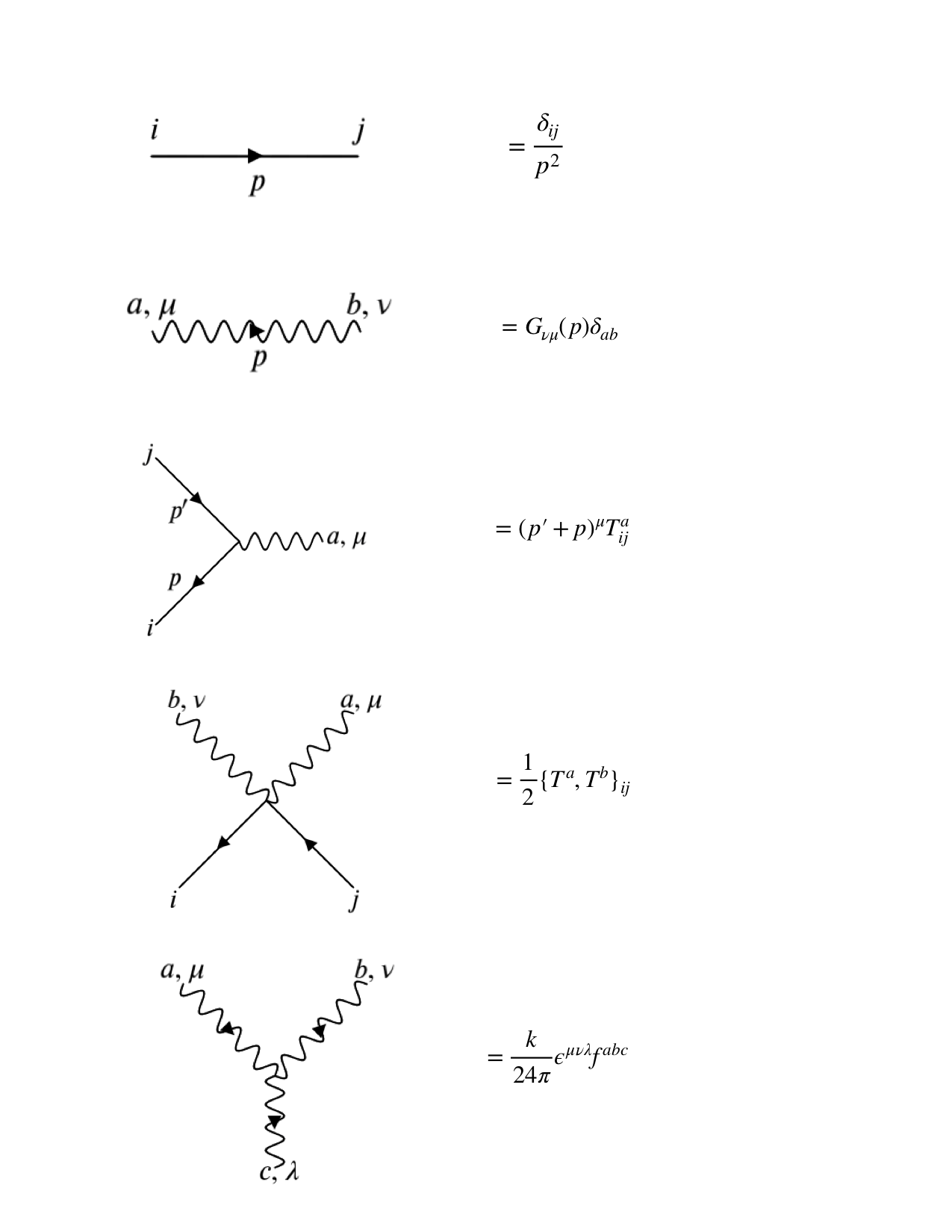
Figure 6: Feynman rules for regular bosonic theory

We obtain the Feynman rules as depicted in Fig. 6. If we work in the Landau gauge, as in Aharony:2011jz , then we have gluon propagator to be as

$$G_{\mu\nu}=-\frac{4\pi}{k}\frac{\epsilon^{\mu\nu\delta}p_{\delta}}{p^{2}}.$$ (61)

Appendix B Two-sided Padé approximation

Let us also observe that our conjecture can be thought of as a two-sided Padé approximation. In this sense, even if our conjecture turns out to be incorrect, it provides a good estimate for the anomalous dimension of the scalar primary that takes into account all known weak-coupling and strong-coupling calculations.

Consider making an $(m,n)$-Padé approximation of $\gamma_{0}$ as follows:

$$\gamma_{0}^{(m,n)}=\frac{A_{0}+A_{2}\tilde{\lambda}_{QB}^{2}+\ldots+A_{m}\tilde{\lambda}_{QB}^{m}}{1+B_{2}\tilde{\lambda}_{QB}^{2}+\ldots+B_{n}\tilde{\lambda}^{n}}.$$ (62)

We only include even powers of $\tilde{\lambda}$ as the anomalous dimension must be parity-invariant.

The $(2,2)$ Padé approximation has three unknowns. We have four perturbative data to constrain it:

• The fact that $\gamma_{0}$ vanishes when $\tilde{\lambda}_{QB}=0$.

• A two-loop calculation $\gamma_{0}$ in the regular-bosonic theory.

• The value of $\gamma_{0}$ in the critical fermionic theory at $\lambda_{b}=0$.

• A two-loop (order $\lambda_{b}^{2}$) calculation of $\gamma_{0}$ in the critical fermionic theory.

Hence the Padé-approximation is overconstrained. Nevertheless, it is possible to fit all four results with following choice of three coefficients.

$$A_{0}=0,~{}~{}A_{2}=-\frac{32}{3\pi^{2}},~{}~{}B_{2}=1.$$ (63)

Repeating the calculation to obtain a $(2,2)$ Padé approximation for the quasi-fermionic theory, we obtain the same coefficients. However, we also have to impose the extra constraint of equation (31), which turns out to be automatically satisfied.

Hence, the simplest Padé approximation to the perturbative data we have seems to work very well. Of course, it is possible to obtain higher-order Padé approximations that satisfy all these constraints, so our answer is not uniquely determined by this procedure. But, it is an interesting observation that, for a variety of physical quantities, such as planar three-point functions MZ , planar four-point function of the scalar primary Turiaci:2018dht , and the $1/N$ higher-spin spectrum Giombi:2016zwa , a relatively simple Padé approximation defined using the variables $\tilde{\lambda}$ and $\tilde{N}$, happens to coincide with the exact answer.

References

- (1) S. Giombi, S. Minwalla, S. Prakash, S. P. Trivedi, S. R. Wadia et al., Chern-Simons Theory with Vector Fermion Matter, Eur.Phys.J. C72 (2012) 2112 [1110.4386].
- (2) O. Aharony, G. Gur-Ari and R. Yacoby, d=3 Bosonic Vector Models Coupled to Chern-Simons Gauge Theories, JHEP 1203 (2012) 037 [1110.4382].
- (3) J. Maldacena and A. Zhiboedov, Constraining conformal field theories with a slightly broken higher spin symmetry, Class.Quant.Grav. 30 (2013) 104003 [1204.3882].
- (4) O. Aharony, G. Gur-Ari and R. Yacoby, Correlation Functions of Large N Chern-Simons-Matter Theories and Bosonization in Three Dimensions, JHEP 1212 (2012) 028 [1207.4593].
- (5) E. Skvortsov, Light-Front Bootstrap for Chern-Simons Matter Theories, JHEP 06 (2019) 058 [1811.12333].
- (6) G. Gur-Ari and R. Yacoby, Correlators of Large N Fermionic Chern-Simons Vector Models, JHEP 1302 (2013) 150 [1211.1866].
- (7) O. Aharony, S. Giombi, G. Gur-Ari, J. Maldacena and R. Yacoby, The Thermal Free Energy in Large N Chern-Simons-Matter Theories, 1211.4843.
- (8) G. Gur-Ari and R. Yacoby, Three Dimensional Bosonization From Supersymmetry, JHEP 11 (2015) 013 [1507.04378].
- (9) A. Bedhotiya and S. Prakash, A test of bosonization at the level of four-point functions in Chern-Simons vector models, JHEP 12 (2015) 032 [1506.05412].
- (10) S. Minwalla and S. Yokoyama, Chern Simons Bosonization along RG Flows, JHEP 02 (2016) 103 [1507.04546].
- (11) O. Aharony, Baryons, monopoles and dualities in Chern-Simons-matter theories, JHEP 02 (2016) 093 [1512.00161].
- (12) O. Aharony, S. Jain and S. Minwalla, Flows, Fixed Points and Duality in Chern-Simons-matter theories, JHEP 12 (2018) 058 [1808.03317].
- (13) S. Yokoyama, Scattering Amplitude and Bosonization Duality in General Chern-Simons Vector Models, JHEP 09 (2016) 105 [1604.01897].
- (14) N. Seiberg, T. Senthil, C. Wang and E. Witten, A Duality Web in 2+1 Dimensions and Condensed Matter Physics, 1606.01989.
- (15) J. Murugan and H. Nastase, Particle-vortex duality in topological insulators and superconductors, 1606.01912.
- (16) S. Kachru, M. Mulligan, G. Torroba and H. Wang, Bosonization and Mirror Symmetry, Phys. Rev. D94 (2016) 085009 [1608.05077].
- (17) D. Radicevic, D. Tong and C. Turner, Non-Abelian 3d Bosonization and Quantum Hall States, 1608.04732.
- (18) P.-S. Hsin and N. Seiberg, Level/rank Duality and Chern-Simons-Matter Theories, JHEP 09 (2016) 095 [1607.07457].
- (19) S. Jain, S. Minwalla, T. Sharma, T. Takimi, S. R. Wadia et al., Phases of large vector Chern-Simons theories on , 1301.6169.
- (20) S. Jain, S. Minwalla and S. Yokoyama, Chern Simons duality with a fundamental boson and fermion, JHEP 1311 (2013) 037 [1305.7235].
- (21) S. Jain, M. Mandlik, S. Minwalla, T. Takimi, S. R. Wadia and S. Yokoyama, Unitarity, Crossing Symmetry and Duality of the S-matrix in large N Chern-Simons theories with fundamental matter, JHEP 04 (2015) 129 [1404.6373].
- (22) S. Giombi, V. Gurucharan, V. Kirilin, S. Prakash and E. Skvortsov, On the Higher-Spin Spectrum in Large N Chern-Simons Vector Models, JHEP 01 (2017) 058 [1610.08472].
- (23) S. Giombi and V. Kirilin, Anomalous Dimensions in CFT with Weakly Broken Higher Spin Symmetry, 1601.01310.
- (24) K. Nii, Classical equation of motion and Anomalous dimensions at leading order, JHEP 07 (2016) 107 [1605.08868].
- (25) E. D. Skvortsov, On (Un)Broken Higher-Spin Symmetry in Vector Models, 1512.05994.
- (26) X.-G. Wen and Y.-S. Wu, Transitions between the quantum hall states and insulators induced by periodic potentials, Phys. Rev. Lett. 70 (1993) 1501.
- (27) W. Chen, M. P. A. Fisher and Y.-S. Wu, Mott transition in an anyon gas, Phys. Rev. B 48 (1993) 13749.
- (28) A. Hui, M. Mulligan and E.-A. Kim, Non-Abelian Fermionization and Fractional Quantum Hall Transitions, 1710.11137.
- (29) A. Hui, E.-A. Kim and M. Mulligan, Non-Abelian bosonization and modular transformation approach to superuniversality, Phys. Rev. B99 (2019) 125135 [1712.04942].
- (30) V. Gurucharan and S. Prakash, Anomalous dimensions in non-supersymmetric bifundamental Chern-Simons theories, JHEP 09 (2014) 009 [1404.7849].
- (31) A. Sen, S-duality Improved Superstring Perturbation Theory, JHEP 11 (2013) 029 [1304.0458].
- (32) L. Avdeev, G. Grigorev and D. Kazakov, Renormalizations in Abelian Chern-Simons field theories with matter, Nucl.Phys. B382 (1992) 561.
- (33) E. Ivanov, Chern-Simons matter systems with manifest N=2 supersymmetry, Phys.Lett. B268 (1991) 203.
- (34) W. Chen, G. W. Semenoff and Y.-S. Wu, Two loop analysis of nonAbelian Chern-Simons theory, Phys.Rev. D46 (1992) 5521 [hep-th/9209005].
- (35) S. Banerjee and D. Radicevic, Chern-Simons theory coupled to bifundamental scalars, JHEP 06 (2014) 168 [1308.2077].
- (36) T. Muta and D. S. Popovic, Anomalous Dimensions of Composite Operators in the Gross-Neveu Model in Two + Epsilon Dimensions, Prog. Theor. Phys. 57 (1977) 1705.
- (37) K. Lang and W. Ruhl, The Critical O(N) sigma model at dimensions 2 ¡ d ¡ 4: Fusion coefficients and anomalous dimensions, Nucl. Phys. B400 (1993) 597.
- (38) A. N. Manashov and E. D. Skvortsov, Higher-spin currents in the Gross-Neveu model at , 1610.06938.
- (39) A. N. Manashov, E. D. Skvortsov and M. Strohmaier, Higher spin currents in the critical ) vector model at , JHEP 08 (2017) 106 [1706.09256].
- (40) G. J. Turiaci and A. Zhiboedov, Veneziano Amplitude of Vasiliev Theory, JHEP 10 (2018) 034 [1802.04390].