Spatio-kinematical model of the collimated molecular outflow in the water-fountain nebula IRAS 16342$-$3814

Abstract

Context. Water fountain nebulae are AGB and post-AGB objects that exhibit high-velocity outflows traced by water maser emission. Their study is important to understand the interaction between collimated jets and the circumstellar material that leads to the formation of bipolar/multi-polar morphologies in evolved stars.

Aims. To describe the three-dimensional morphology and kinematics of the molecular gas of the water-fountain nebula IRAS 16342$-$3814.

Methods. Retrieving data from the ALMA archive to analyse it using a simple spatio-kinematical model. Using the software SHAPE to construct a three-dimensional spatio-kinematical model of the molecular gas in IRAS 16342$-$3814. Reproducing the intensity distribution and position-velocity diagram of the CO emission from the ALMA observations to derive the morphology and velocity field of the gas. Using CO($J$=1$\rightarrow$0) data to support the physical interpretation of the model.

Results. A spatio-kinematical model that includes a high-velocity collimated outflow embedded within material expanding at relatively lower velocity reproduces the images and position-velocity diagrams from the observations. The derived morphology is in good agreement with previous results from IR and H₂O maser emission observations. The high-velocity collimated outflow exhibits deceleration across its length, while the velocity of the surrounding component increases with distance. The morphology of the emitting region; the velocity field and the mass of the gas as function of velocity are in excellent agreement with the properties predicted for a molecular outflow driven by a jet. The timescale of the molecular outflow is estimated to be $\sim$70-100 years. The scalar momentum carried by the outflow is much larger than it can be provided by the radiation of the central star. An oscillating pattern was found associated to the high-velocity collimated outflow. The oscillation period of the pattern is $T$$\approx$60-90 years and its opening angle is $\theta_{\rm op}$$\approx$2^∘.

Conclusions. The CO ($J$=3$\rightarrow$2) emission in IRAS 16342$-$3814 is interpreted in terms of a jet-driven molecular outflow expanding along an elongated region. The position-velocity diagram and the mass spectrum reveal a feature due to entrained material that is associated to the driving jet. This feature is not seen in other more evolved objects that exhibit more developed bipolar morphologies. It is likely that the jet in those objects has already disappeared since it is expected to last only for a couple of hundred years. This strengthens the idea that water fountain nebulae are undergoing a very short transition during which they develop the collimated outflows that shape the CSE. The oscillating pattern seen in the CO high-velocity outflow is interpreted as due to precession with a relatively small opening angle. The precession period is compatible with the period of the corkscrew pattern seen at IR wavelengths. We propose that the high-velocity molecular outflow traces the underlying primary jet that produces such pattern.

1 Introduction

There is a growing consensus that collimated jet-like outflows create cavities with dense walls in the slowly expanding circumstellar envelopes (CSE) of post-Asymptotic Giant Branch (post-AGB) stars. Once the central star becomes hot enough to ionise the circumstellar material, such structures are seen as beautiful and colourful bipolar or even multi-polar planetary nebulae (PNe) (Sahai & Trauger 1998). Water-fountain nebulae (wf-nebulae) are a reduced group of AGB and post-AGB objects that are thought to be experiencing the first manifestation of such collimated outflows (Imai 2007). Therefore these objects are one of the best tools that we have available to probe and study the mechanisms of jet launching and collimation in evolved stars, as well as the interaction of the jet with the CSE.

IRAS 16342$-$3814 was the first object to be classified as a wf-nebula given the wide spread of its H₂O maser emission of $\sim$260 km s^-1 (Likkel & Morris 1988). IRAS 16342$-$3814 is one of the best studied wf-nebulae, observed over a wide range of wavelengths across the electromagnetic spectrum, from optical to radio (Sahai et al. 1999, 2005; Gledhill & Forde 2012; Imai et al. 2012; Sahai et al. 2017). The distribution and kinematics of the circumstellar material has also been studied via its H₂O and OH maser emission (Claussen et al. 2009; Sahai et al. 1999).

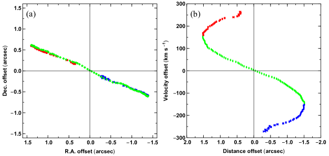
Figure 1: (a) Peak positions of the brightness distribution of CO(3$\rightarrow$2) emission for each individual velocity channel obtained with the task JMFIT of AIPS. The origin corresponds to the non-weighted mean position of the distribution (see main text). The negative R.A. offsets are on the right side of the plot. (b) Distance offsets from the mean position as a function of the velocity offset from the systemic velocity v_sys,LSR=45 km s^-1. The colour of the data points are coded according to their velocity gradient, $|$dv$|$/$|$dr$|$; green for $|$dv$|$/$|$dr$|$¿0 and blue-red for $|$dv$|$/$|$dr$|$¡0. The negative distance offsets correspond to data points with negative R.A. offsets and they are on the right side of the plot. The error bars of the positions are included in the plot but their sizes is similar to the size of the data points.

The Hubble Space Telescope (HST) and Keck Adaptive Optics (AO) images of IRAS 16342$-$3814 show a small (3^′′) bipolar nebula, with the lobes separated by a dark equatorial waist (Sahai et al. 1999, 2005). The morphology seen in the images implies that the lobes are bubble-like reflection nebulae illuminated by starlight escaping through polar holes in a dense, dusty waist obscuring the central star. The AO observations reveal a corkscrew-shaped pattern apparently etched into the lobe walls, which is inferred to be the signature of an underlying precessing jet. This jet has presumably carved out the observed bipolar cavities in the surrounding envelope formed during the AGB phase of the star (Sahai et al. 2005). Gledhill & Forde (2012) studied the H₂ emission of this source and concluded that it is likely that the jet and outflow are powered by accretion onto a binary companion. The water masers in IRAS 16342$-$3814 are thought to be tracing bow shocks at the ends of a jet. From the analysis of the proper motions of the masers Claussen et al. (2009) derived an expansion velocity for the material in the head of the jet of v_exp$\sim$155-180 km s^-1.

Recently, Sahai et al. (2017) carried out observations of the molecular emission of IRAS 16342$-$3814 with ALMA. From the results of their observations these authors concluded that the emission originates in a precessing molecular outflow with a wide precession angle of $\sim$90^∘. However, it is difficult to explain the creation of an outflow with such a wide precession angle by the jet underlying the corkscrew pattern seen from the AO observations. In this work we present a different spatio-kinematical model of the collimated molecular outflow in the water-fountain nebula IRAS 16342$-$3814 that considers a small opening angle, which is in better agreement with the results from previous observations.

2 CO ALMA data of IRAS 16342$-$3814

We retrieved archive ALMA data of the project 2012.1.00678.S (PI: R. Sahai) to study in more detail the kinematics of the molecular gas in IRAS 16342$-$3814. The spectral setup, sensitivity, angular resolution and results of the observations of the CO($J$=3$\rightarrow$2), ¹³CO($J$=3$\rightarrow$2) and H¹³CO($J$=4$\rightarrow$3) emission lines were reported by (Sahai et al. 2017). In this work we further analyse the kinematics of the molecular gas using the emission from the CO($J$=3$\rightarrow$2) line, as this emission line has the highest signal-to-noise ratio. Since the position-velocity (P-V) diagrams of the ¹³CO($J$=3$\rightarrow$2) and H¹³CO($J$=4$\rightarrow$3) are very similar to that of the CO($J$=3$\rightarrow$2) line, the main results presented in this work are valid for the three lines.

In addition to the archival data, we have also obtained data from ALMA observations of the CO($J$=1$\rightarrow$0) line. These observations are part of the project 2018.1.00250.S (PI: D. Tafoya) and were carried out on December 9 2018 using 43-12m antennas with a maximum and minimum baselines of 740 m and 15 m, respectively. The resulting angular resolution was around 1^′′ and the maximum recoverable scale was 11$\hbox to0.0pt{.\hss}^{\prime\prime}$8. The data were calibrated with the ALMA pipeline using the CASA version 5.4.0-68. Subsequently, the data were self-calibrated in phase following the standard self-calibration guidelines for ALMA data. In the present work, the observations of the CO($J$=1$\rightarrow$0) line are used mainly to support the conclusions drawn from the CO($J$=3$\rightarrow$2) emission (see §4), but they will be presented and discussed in more detail somewhere else.

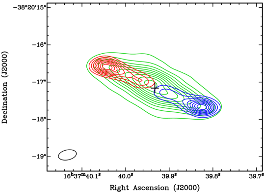
Figure 2: Velocity integrated CO($J$=3$\rightarrow$2) emission of IRAS 16342$-$3814. The blue, green and red contours correspond to emission at velocity ranges $-$270¡v_offset(km s^-1)¡$-$150, $-$150¡v_offset(km s^-1)¡+150; and +150¡v_offset(km s^-1)¡+270, respectively (see main text). The levels of the blue and red contours go from 20% to 90% the peak value of the emission (8.3 and 6.6 Jy beam^-1 km s^-1, respectively) at steps of 10%. The levels of the green contours go from 5% to 95% the peak value of the emission (50.7 Jy beam^-1 km s^-1) at steps of 10%. The rms value of the velocity-integrated maps is $\sim$7$\times$10^-2 Jy beam^-1 km s^-1. The cross indicates the peak of the continuum emission. The ellipse located at the lower left corner indicates the synthesised beam, $\theta_{\rm FWHM}$=0$\hbox to0.0pt{.\hss}^{\prime\prime}$49$\times$0$\hbox to0.0pt{.\hss}^{\prime\prime}$27, P.A.=$-$78^∘

.

From the data cube of the CO($J$=3$\rightarrow$2) line we extracted the peak position of the brightness distribution in every channel within the velocity range $-235$¡v_LSR(km s^-1)¡+325 using the task JMFIT of AIPS. The emission within this velocity range corresponds to the high velocity outflow (HVO) observed by Sahai et al. (2017), see their Figs. 1b and 2. It should be noted that apart from this emission, Sahai et al. (2017) also identified an extreme high-velocity outflow (EHVO) with higher expansion velocities. However, here and in the following sections we will only consider the emission associated to the HVO and leave the discussion of the nature of the EHVO for §4.2. From the measured peak positions of the CO($J$=3$\rightarrow$2) emission we estimated the centroid of the distribution by computing the non-weighted mean value. The position of the centroid was used as a reference position throughout the analysis described below. In Fig. 1a we plot the declination (Dec.) and right ascension (R.A.) offsets of the emission peak positions with respect to the reference position. Subsequently, we calculated the separation of the emission peak positions to the reference position as Dist.offset=$\pm$$\sqrt{{\rm R.A.offset}^{2}+{\rm Dec.offset}^{2}}$. We used the minus sign when R.A. offset was negative, otherwise we used the plus sign. In Fig. 1b we plot the distance-offset of the emission peak position as a function of the velocity-offset of the channel. The velocity-offsets are defined with respect to the systemic velocity of the source, assumed to be v_sys,LSR=45 km s^-1 (Sahai et al. 2017). The data points are colour-coded according to their velocity gradient, $|$dv$|$/$|$d$r$$|$; green for $|$dv$|$/$|$d$r$$|$¿0 and blue-red for $|$dv$|$/$|$d$r$$|$¡0 (see below). The distribution of the points in the plot of Fig. 1b exhibits an S-like shape similarly to the emission in the P-V diagram obtained by Sahai et al. (2017) (see Fig. 2 of Sahai et al. 2017). This is due to the fact that the plot shown in Fig. 1b is equivalent to a P-V diagram since the emission peak positions lie basically along one single direction on the sky (P.A. $\sim$67^∘, see Fig. 1a).

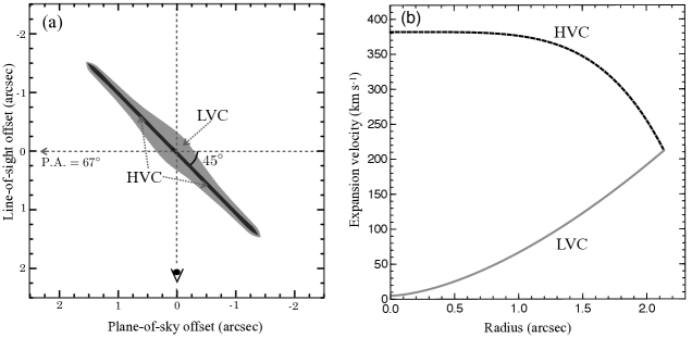
Figure 3: (a) Geometry of the spatio-kinematical model of the molecular envelope of IRAS 16342$-$3814. Note that the y-axis is angular size along the line-of-sight and the x-axis is angular size on the plane of the sky. We assume an inclination of the major axis of the nebula of 45^∘ with respect to the plane of the sky (Claussen et al. 2009). The grey region indicates the LVC component. The black region indicates the HVC component. (b) Expansion velocity as a function of the separation from the center of the system. The grey and black lines are the velocity laws for the LVC and HVC components, respectively. The mathematical expression for the velocity laws is given in Equation 1.

From the plot of Fig. 1b it can be seen that for velocities —v_offset—¡150 km s^-1 the absolute value of the velocity offset increases monotonically as a function of the absolute distance offset, $|$dv$|$/$|$dr$|$¿0. For —v_offset—¿150 km s^-1 the gradient is opposite, $|$dv$|$/$|$dr$|$¡0. Therefore, this plot suggests the presence of different molecular gas components with different kinematical signatures, which are indicated with green and blue-red colours, respectively. We will refer to these components as kinematical components. In the following we consider these two types of kinematical components, one with positive velocity gradient and the other with negative velocity gradient. Surprisingly, as the plot of Fig. 1a shows, even though these components have different kinematical signatures, they are almost perfectly aligned on one single direction on the plane of the sky.

In order to visualise the spatial distribution of the emission of the kinematical components defined above, we created velocity-integrated images of the CO($J$=3$\rightarrow$2) emission taking into account their corresponding velocity ranges. We considered three velocity ranges as follows: $-$150¡v_offset(km s^-1)¡+150; $-$270¡v_offset(km s^-1)¡$-$150 and +150¡v_offset(km s^-1)¡+270. The first velocity range corresponds to the kinematical component with positive velocity gradient while the two last ones correspond to the kinematical component with negative velocity gradient.

In Fig. 2 we show contour maps of the integrated CO($J$=3$\rightarrow$2) emission obtained from the velocity ranges considered above. The blue contours indicate emission integrated over the velocity range $-$270¡v_offset(km s^-1)¡$-$150; the green contours indicate emission integrated over the velocity range $-$150¡v_offset(km s^-1)¡+150, and the red contours indicate emission integrated over the velocity range +150¡v_offset(km s^-1)¡+270. Note that this colour coding is the same as the one for the kinematical components shown in Fig. 1. From Fig. 2 it can be seen that the emission with velocity-offsets —v_offset—¿150 km s^-1, from now on referred to as high-velocity emission, traces a pair of collimated bipolar lobes along the direction with P.A.=$\sim$67^∘. The velocity-integrated intensity of the high-velocity emission has two emission peaks located at the tips of the bipolar lobes. The geometric centre of the bipolar lobes coincides with the central part of the nebula, which is indicated with a cross that corresponds to the peak position of the continuum emission, (J2000) R.A.=16:37:39.935, Dec.=$-$38:20:17.15. The structure traced by emission with velocity offsets —v_offset—¡150 km s^-1, from now on referred to as low-velocity emission, exhibits a more extended morphology encompassing the high-velocity emission. The low-velocity emission has only one intensity peak located near the centre of the system. The width of the brightness distribution of the low-velocity emission decreases along the direction of the bipolar axis resembling an elongated diamond-like shape.

3 Spatio-kinematical model of the molecular gas

In this section we present a simple spatio-kinematical model of the molecular gas of IRAS 16342$-$3814 to reproduce the spatial distribution and velocity gradients seen in Figs. 1 and 2. In the following we describe the considerations that we made to define the morphology and velocity field used in our model. First we note from Fig.  1a that the spatial distribution of the emission peak positions of the kinematical components, defined in §2, lie along one single direction on the plane of the sky. This could be due to the kinematical components being intrinsically aligned on one single direction, or alternatively they could lie on different directions but appear perfectly aligned on the plane of the sky. We consider that the latter possibility is very unlikely as even a small inclination of the system with respect to the line-of-sight would result in the components appearing misaligned on the plane of the sky. Furthermore, previous observations suggest that the gas and dust are located within a narrow cone elongated along the direction with P.A.$\sim$67^∘ (Sahai et al. 2005; Claussen et al. 2009; Imai et al. 2012; Gledhill & Forde 2012). Therefore, in this work we adopt a geometry similar to the one assumed in previous works and propose that the observed CO($J$=3$\rightarrow$2) emission can be explained using two morphological structures associated to the kinematical components defined in §2: i) an elongated structure with a relatively wide waist and narrow tips. This component is associated with the low-velocity emission and we will refer to it as the low-velocity component (LVC). ii) A pencil-like collimated structure associated with the high-velocity emission that lies embedded within the LVC component. We will refer to this component as the high-velocity component (HVC). Thus, the morphology for the CO emitting region of IRAS 16342$-$3814 in our spatio-kinematical model has a shape that resembles a French spindle, as it is shown in Fig. 3a.

The width of the LVC, as a function of the velocity, was determined by fitting a two-dimensional Gaussian function to the intensity distribution in each individual channel of the data cube. The size was set equal to the quadratic average of the major and minor axis, deconvolved from the beam, of the fitted elliptical Gaussian function. The width of this component, at its waist, is $\sim$0$\hbox to0.0pt{.\hss}^{\prime\prime}$5 and it decreases monotonically to reach a value of $\sim$0$\hbox to0.0pt{.\hss}^{\prime\prime}$15 at the polar tips. The width of the HVC is not resolved by these observations but we adopted a width at the equator of $\sim$0$\hbox to0.0pt{.\hss}^{\prime\prime}$02 and set it to increase monotonically to a value of $\sim$0$\hbox to0.0pt{.\hss}^{\prime\prime}$05 based on the opening angle of the sinusoidal distribution of the peak positions of this component (see §4.2 and Fig. 8). The major axis of both components was assumed to have an inclination angle with respect to the plane of the sky $\theta_{\rm inc}$=45^∘, which Claussen et al. (2009) obtained by measuring the inclination angle of the three-dimensional velocity vectors of the H₂O masers. It is worth mentioning that an independent estimate of the inclination angle of $\sim$40^∘ was obtained by Sahai et al. (1999) from observations of OH masers. However, we opted for the value derived by Claussen et al. (2009) because it was obtained in a more straightforward manner. The de-projected length along the major axis of both components was estimated from the maximum separation of the emission peak positions from the reference position (see Fig. 1b), $r_{\rm max}$=1$\hbox to0.0pt{.\hss}^{\prime\prime}$5/cos $\theta_{\rm inc}$=2$\hbox to0.0pt{.\hss}^{\prime\prime}$12. In this work we adopt a distance to IRAS 16342$-$3814 $D$=2 kpc (Sahai et al. 1999). To express the expansion velocity field of the molecular gas we used a power-law function given by the following equation:

$$\left[\frac{{\rm v}_{\rm exp}(r)}{{\rm km\leavevmode\nobreak\ s}^{-1}}\right]={\rm v}_{\rm i}-({\rm v}_{\rm i}-{\rm v}_{\rm f})\times\left(\frac{r}{r_{\rm max}}\right)^{\eta},$$ (1)

where v_i (initial velocity) is the value of the expansion velocity at $r$=0; v_f (final velocity) is the value of the velocity at the tips of the lobes, and $\eta$ is the exponent of the power-law function.

Figure 4: (a) Mesh representation of the spatial distribution of the molecular outflow of IRAS 16342$-$3814. The HVC and LVC are shown in black and grey colours, respectively. The vectors represent the expansion velocity of the gas and they are coloured according to their component in the line-of-sight. (b) Brightness distribution of the CO emission obtained from the render function of SHAPE. The intensity is given in arbitrary units. The synthetic image was convolved with a Gaussian function with FWHM similar to the synthesised beam of the observations. The parallel lines at P.A.=67^∘ indicate the direction of a slit used to generate the synthetic P-V diagram shown in Fig. 5a.

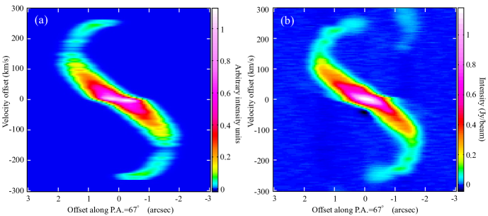
Figure 5: (a) P-V diagram of IRAS 16342$-$3814 obtained from our SHAPE model. (b) P-V diagram of IRAS 16342$-$3814 from the ALMA observations. The faint emission in the upper-right corner is due to the H¹³CO($J$=4$\rightarrow$3) line. Both P-V diagrams were obtained using a slit along P.A.=67^∘

The values of the initial and final velocity for the HVC can be obtained from the maximum and minimum value of the velocity range of its corresponding kinematical component, i.e. 150¡—v_offset (km s^-1)—¡270 (see §2). Thus, taking into account the inclination angle, v_i,HVC=270 km s^-1/sin $\theta_{\rm inc}$=382 km s^-1 and v_f,HVC=150 km s^-1/sin $\theta_{\rm inc}$=212 km s^-1. Given that the data points in Fig. 1b exhibit a continuous transition between the two kinematical components, we set the final velocity of the LVC equal the the final velocity of the HVC, i.e. v_f$\equiv$v_f,LVC=v_f,HVC. The initial velocity for the LVC, ${\rm v}_{\rm i,LVC}$, cannot be directly obtained from the observations. From the plot of Fig. 1b it can be seen that ${\rm v}_{\rm exp}$($r$=0)$\approx$0, but the points in this plot represent an average position of the distribution of the emission for a certain velocity offset. Therefore, the point located at the origin of coordinates, (v=0, $r$=0), does not necessarily indicate that v_exp=0 when $r$=0, but it means that the average position of the emission is equal to zero in the channel with v_offset=0. Consequently, v_i,LVC was left as a free parameter, together with the exponents of the power-law functions, to be adjusted by further comparison of our model with the observations.

3.1 3D modelling with SHAPE

We used the spatio-kinematic modelling tool SHAPE (Steffen et al. 2011) to construct a three-dimensional (3D) version of our model of the distribution and kinematics of the molecular gas in IRAS 16342$-$3814 and compare it with the observations. It should be remarked that this model is not meant to reproduce the emission of any particular molecular line but it only illustrates the overall behaviour of the radiation arising within the kinematical components. First we obtained synthetic images and P-V diagrams of our spatio-kinematical model with SHAPE using initial guess values. Subsequently, we compared the results of SHAPE with the observations in an iterative approach to derive the values of the free parameters of our model (see below). The synthetic P-V diagram obtained with SHAPE and the one from the observations were compared by eye. After several iterations we found a good fit to the observations using the following parameters for the power-law function: v_i,HVC=382 km s^-1, v_f,HVC=212 km s^-1 and $\eta_{\rm HVC}$=4.5 for the HVC; v_i,LVC=5 km s^-1, v_f,LVC=212 km s^-1 and $\eta_{\rm LVC}$=1.6 for the LVC. The power-law functions for both components are shown in the plot of Fig. 3b.

Fig. 4a shows a mesh view of the 3D morphology of the emitting region used in SHAPE. The grey and black meshes represents the LVC and HVC components, respectively. The arrows represent vectors of the velocity field of the expanding gas. The colours of the velocity vectors are coded according to their component in the line-of-sight direction. We performed a simple radiative transfer of our model using the physical render function of SHAPE, thus the emerging emission is proportional to $T_{\rm ex}(1-e^{-\tau_{\nu}})$, where $T_{\rm ex}$ is the excitation temperature and $\tau_{\nu}$ is the optical depth. The LTE option in SHAPE was turned on, which calculates the absorption/emission ratio assuming Local Thermodynamic Equilibrium conditions, and the absorption coefficient was defined so that $\tau_{\nu}$ is proportional to the product of the gas density and the length of the emitting region along the line-of-sigh, $\tau_{\nu}\propto n$$\times$$l$. For simplicity, the density of the gas and the excitation temperature of the HVC were assumed to be constant throughout the outflow. At the base of the LVC, the excitation temperature was set to a value 5 times lower than the HVC, increasing monotonically as a function of the distance to reach the same value as the HVC at the tip of the lobes. We aware the reader that it is not the scope of this work to perform a detailed radiative transfer analysis of the model but we are only concerned about the kinematics of the gas. Therefore, the resulting intensity of the synthetic images is given in arbitrary units and do not necessarily correspond to the intensity of the observed emission. The synthetic images were convolved with a Gaussian function with FWHM similar to the synthesised beam of the observations.

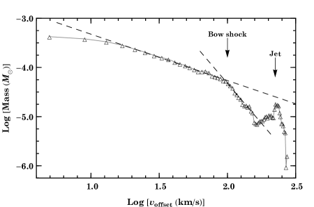
Figure 6: Molecular mass as a function of expansion velocity obtained from the emission blue-shifted with respect to the systemic velocity. The dashed lines are power-law fits to the data in the velocity ranges 10¡v_offset(km s^-1)¡100 and 100¡v_offset(km s^-1)¡150, respectively. The arrows indicate the emission associated with the bow shock and the jet, respectively (see main text).

In Fig. 4b we show a synthetic image of the emission of the source on the plane of the sky. The spatial distribution of the emission of our model resembles the image of the HVO of IRAS 16342$-$3814 obtained by Sahai et al. (2017) (see Fig. 2b of Sahai et al. 2017). The two parallel lines in Fig. 4b indicate the direction of a slit used to generate the synthetic P-V diagram shown in Fig. 5a. We used a similar slit to generate a P-V diagram from the data cube of the CO($J$=3$\rightarrow$2) emission, which is shown in Fig. 5b. The faint emission in the upper-right corner of the P-V diagram of Fig. 5b is due to the H¹³CO($J$=4$\rightarrow$3) line overlapping in frequency with the CO($J$=3$\rightarrow$2) emission (see also Figure 3 of Sahai et al. 2017). The synthetic P-V diagram in Fig. 5a reproduces very well the main features of the CO($J$=3$\rightarrow$2) emission P-V diagram. The clumpy structure that some parts of the synthetic P-V diagram exhibit is due to the binning of the velocity channels during the convolution of the model.

4 Discussion and interpretation of the spatio-kinematical model

Sahai et al. (2017) proposed a model to explain the P-V diagrams of the CO($J$=3$\rightarrow$2) and H¹³CO($J$=4$\rightarrow$3) emission assuming that all the molecular gas is expanding with the same intrinsic velocity. In their model, the S-like pattern seen in the P-V diagram results from the projection effect of the material moving along different directions with respect to the line-of-sight. Under this assumption they concluded that the morphology of the source is a S-like bipolar shape with some gas clouds expanding in directions near the line-of-sight and some other ones near the plane of the sky (see Fig. 3 of Sahai et al. 2017). This model has two main problems: i) The constant expansion velocity assumption is most likely not true, since the velocity of the gas would depend on the hydrodynamic interaction of the driving jet and the CSE, as Sahai et al. (2017) acknowledge. ii) The morphology of the nebula derived from this assumption may result in an S-like shape with a very wide opening angle ($\sim$90^∘) that would not be consistent with the highly collimated morphologies suggested by the IR observations and the H₂O masers. However, we note that a possible resolution to the problem in item (ii) is provided by the Spiral-class PNe introduced by Sahai et al. (2011) (e.g. PK 032+07#2 and PNG 356.8+0.3.3, see Fig. 7 of Sahai et al. 2011), which, if viewed at a preferred orientation angle, could resemble the lobes seen in IRAS 16342$-$3814.

In the previous section, §3, we showed that the spatio-kinematical model presented in this work reproduces very well the distribution of the observed CO($J$=3$\rightarrow$2) emission in the P-V diagram. As discussed above, the gradients seen in the P-V diagram (Fig. 5b) are interpreted as being due to actual variations of the velocity field of the gas within an elongated narrow region. Therefore, our model circumvents the problem of assuming a constant expansion velocity and reconciles the morphology of the CO gas with the morphology of the source derived from other observations. In the following we discuss on the astrophysical origin of the observed velocity gradients. In the past three decades a wealth of observations toward regions of star formation, as well as toward evolved stars, have revealed that the main properties that characterise collimated molecular outflows are: i) The velocity field of the outflow is described by a proportional relationship between the expansion velocity and the distance to the driving source, i.e. v$\propto$$r^{\eta}$, with $\eta$$\approx$1. ii) The collimation of the flow increases systematically with flow velocity and distance from the driving source. iii) The flow exhibits a power-law variation of mass with velocity, i.e. $m(\rm v)$$\propto$v^-γ (Lada & Fich 1996; Cabrit et al. 1997, and references therein). The most popular mechanism to explain these properties is the jet-driven bow shock (Raga & Cabrit 1993; Smith et al. 1997). This mechanism naturally creates a positive velocity gradient since as one moves from the broader wings to the narrow apex of the bow shock the shock becomes less oblique and the net forward velocity increases. In addition, this mechanism produces more swept-up mass at low velocities since the intercepted mass flux is determined by the bow shock cross-section, which steadily grows in the bow wings while the velocity decreases (Cabrit et al. 1997). The LVC of IRAS 16342$-$3814 exhibits all the properties that characterise jet-driven bow shocks. As shown in §3, the velocity field of the LVC has a power-law dependence with the distance, although the power-law exponent, $\eta$=1.6, is somewhat larger than the typical values seen in other molecular outflows. The collimation of the LVC increases with velocity as it can be seen in Fig. 2. Finally, assuming optically thin emission, LTE conditions and an average excitation temperature $T_{\rm ex}$=30 K, the mass of gas expanding at a given velocity, i.e. the mass spectrum $m$(v), can be obtained from the line profile of the CO($J$=3$\rightarrow$2) emission. In Fig. 6 we show a log-log plot of the mass as a function of the velocity offset, where we have used a fractional abundance of CO relative to H₂, $f$(CO)=3$\times$10^-4 (Sahai et al. 2017). This plot reveals that the emission between 10¡v_offset(km s^-1)¡100 km s^-1 is described by a power-law $m$(v)$\propto$v^-γ with $\gamma$=0.94, and between 100¡v_offset(km s^-1)¡150 km s^-1 $\gamma$=3.2. This double power-law variation of the mass with velocity is exactly what observations have revealed in other molecular outflows (Kuiper et al. 1981; Rodriguez et al. 1982; Lada & Fich 1996), and confirmed by numerical simulations of jet-driven molecular outflows (Smith et al. 1997). However, it should be pointed out that, if the CO($J$=3$\rightarrow$2) line is optically thick, the values of these power-law exponents represent just a lower limit. Furthermore, it cannot be ruled out that the break of the power-law exponent around v_offset=100 km s^-1 might be due to a change in the optical depth regime.

In Fig. 7 we show contours indicating the CO($J$=1$\rightarrow$0) emission superimposed on a moment-8 (maximum value of the spectrum for each pixel) image of the CO($J$=3$\rightarrow$2) emission. The CO($J$=1$\rightarrow$0) emission was averaged over the velocity range $-$10¡v_offset(km s^-1)¡+10, which is the typical expansion velocity of the CSE formed during the AGB phase. The brightness distribution of the emission is round and has a deconvolved size of $\sim$0$\hbox to0.0pt{.\hss}^{\prime\prime}$9, which is almost twice as large as the deconvolved size of the CO($J$=3$\rightarrow$2) emission in the same velocity range (see §3), suggesting that it is tracing material of the CSE created by the AGB wind. The existence of a relic AGB circumstellar envelope is also suggested by the low-velocity OH 1612 maser emission, which exhibits maser features distributed over a region more extended than the bipolar outflow (see Fig. 1 of Sahai et al. 1999). Moreover, Murakawa & Izumiura (2012) showed that the SED of IRAS 16342$-$3814 is best reproduced by a model that includes a disk, a torus, bipolar lobes, as well as a spherical AGB envelope. Thus, given these arguments, together with the results presented in the previous paragraph, we conclude that the LVC in IRAS 16342$-$3814 corresponds to material of the CSE that has been swept-up by the jet-driven bow shock.

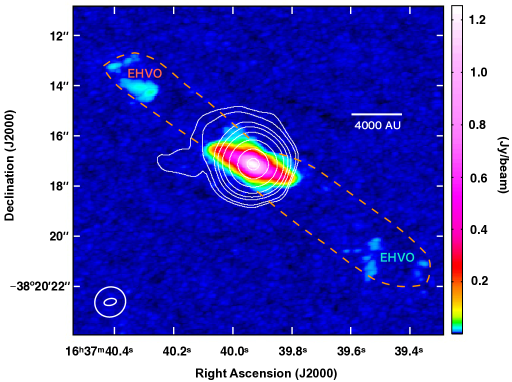
Figure 7: CO emission from IRAS 16342$-$3814. The colour scale corresponds to the moment-8 (maximum value of the spectrum for each pixel) image of the CO($J$=3$\rightarrow$2) emission. The contours indicate the CO($J$=1$\rightarrow$0) emission averaged over the velocity range $-$10¡v_offset(km s^-1)¡+10 with values (0.007, 0.01, 0.02, 0.03, 0.05, 0.1, 0.2, 0.3) Jy beam^-1, where the first contour represents 4 times the value of the rms. The orange dashed line delineates the region that contains emission from the EHVO. The ellipses located at the lower left corner indicate the synthesised beams of the CO($J$=3$\rightarrow$2) and CO($J$=1$\rightarrow$0) observations, respectively. The beam size of the CO($J$=3$\rightarrow$2) observations is the same as in Fig. 2 and the beam size of the CO($J$=1$\rightarrow$0) observations is 1$\hbox to0.0pt{.\hss}^{\prime\prime}$25$\times$1$\hbox to0.0pt{.\hss}^{\prime\prime}$18 with P.A.=$-$58^∘.

A feature revealed in these ALMA observations, not commonly found so evident in other molecular outflows, is the emission associated to the HVC. Fig. 6 shows that for velocities offsets higher than 150 km s^-1 the mass spectrum exhibits a plateau followed by a sharp peak. Smith et al. (1997) obtained a similar feature in the intensity profile from their hydrodynamic simulations of a jet-driven outflow. They identified this feature with the jet’s direct emission (see Fig. 1 and 2 of Smith et al. 1997). The deceleration of these component suggests the presence of turbulent mixing through Kelvin-Helmholtz instabilities at the velocity shear between the jet and the ambient gas. If turbulent entrainment along the beam is the dominant process, then the jet decreases in average velocity along its length as it transfers momentum to the entrained material (Chernin et al. 1994). Given a velocity of the jet v_exp=380 km s^-1, a sound speed in the medium $c_{s}$$\sim$1 km s^-1, a density of the medium $n_{\rm H_{2}}$=10⁶ cm^-3 and a kinetic temperature $T_{\rm k}$$\sim$100 K, the Reynolds number of the jet is $\mathcal{R}e_{m}$¿10¹⁰. Consequently, the jet is expected to be highly turbulent and suffer deceleration, which is indeed what the observations reveal. We conclude that the HVC represents material entrained by the underlying jet near its axis or it could be the molecular component of the jet itself.

As mentioned earlier, molecular outflows with the characteristic properties of a jet-driven outflow have also been found in the CSE of some evolved stars (e.g. Bujarrabal et al. 1998; Sánchez Contreras et al. 2000; Alcolea et al. 2001, 2007). For these objects, the linear relationship between the expansion velocity and the distance to the driving source has been interpreted in terms of free expansion of the gas after having suffered a strong axial acceleration by a collimated wind or jet during a time period much shorter than the whole post-AGB lifetime of the source (Bujarrabal et al. 1998; Alcolea et al. 2001). Particularly, Alcolea et al. (2001) derived an upper limit to the duration of this post-AGB interaction in the pre-PN OH 231.8$+$4.2 of $\sim$125 years. Our results suggest that in IRAS 16342$-$3814 we are witnessing the presence of two different processes of entrainment, one called “prompt entrainment”, which transfers momentum through the leading bow shock, and the second is “steady-state entrainment”, which refers to ambient gas that is entrained along the sides of the jet (De Young 1986; Chernin et al. 1994). The former would lead to the formation of the linear relationship of the velocity with the distance seen in the PV diagrams of the molecular emission of the more evolved objects, which corresponds to swept-up material in a jet-driven bow shock. The new ingredient revealed in these ALMA observations is the HVC, which is related to the driving jet. It is likely that in the molecular outflows seen in other more evolved objects the jet has long disappeared as it is expected to last only for a couple of hundred years. This strengthens the idea that wf-nebula are indeed undergoing the ephemeral transition where they develop the collimated outflows that shape the CSE leading to the formation of asymmetrical PNe. In fact, recently Orosz et al. (2018) showed a beautiful example of a decelerating outflow in the wf-nebula IRAS 18113$-$2503 traced by H₂O masers, which is likely to be directly related to the driving jet.

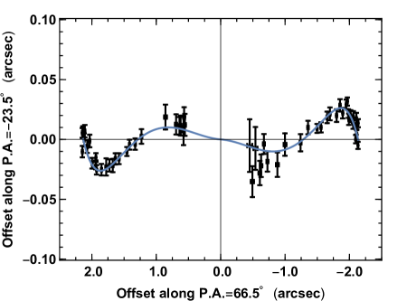
Figure 8: Oscillating pattern of the positions of the peak-emission for the high-velocity emission. The blue line indicates a sinusoidal function fit to the data using Equation 2.

4.1 Timescale of the molecular jet and the equatorial waist

The plot on Fig. 3b and the P-V diagram in Fig. 5b show an instantaneous picture of the velocity field in the outflow at present time. Thus they cannot be used to trace the velocity history of the individual gas particles, unless the deceleration law as a function of time is known. In order to understand the evolution of the P-V diagram as a function of time an entire knowledge of the complex dynamical system of the outflow is required. Consequently, it is difficult to estimate the exact lifetime of the outflow. However, if we make the reasonable assumption that the jet has been launched at roughly the same speed throughout its lifetime, it is clear that the gas particles located at the head of the jet suffered a deceleration from the initial velocity, v_i, to the final velocity, v_f, across its length, $r_{\rm max}$. If we consider a constant deceleration function, the lifetime of the outflow can be obtained as $\tau_{\rm jet}$=2$\times$$r_{\rm max}/({\rm v}_{\rm i}+{\rm v}_{\rm f})$$\approx$70 years. This value is just a lower limit for the lifetime as it is likely that the jet suffered a steeper deceleration in a region closer to the star, where the density of the CSE is larger. For example, if the head of the jet decelerated to its current value, v_f, soon after it was launched and it has been expanding at nearly constant velocity afterwards, the lifetime of the jet is $\tau_{\rm jet}$=$r_{\rm max}/{\rm v}_{\rm f}$$\approx$100 years.

Sahai et al. (2017) identified a toroidal structure in IRAS 16342$-$3814 from the emission of the H¹³CO(4$\rightarrow$3) line and derived a radius $r_{\rm torus}$$\approx$0$\hbox to0.0pt{.\hss}^{\prime\prime}$33 and an expansion velocity of v_torus=20 km s^-1, which gives an expansion timescale of the torus $\tau_{\rm torus}$$\approx$160 years. This value is larger than the timescale of the jet derived above. However, this timescale is obtained assuming that the gas of the torus expanded at constant velocity. According to our interpretation of the LVC (see §4), this toroidal structure would correspond to shocked gas in the equatorial region expanding perpendicularly to the jet (see e.g. Soker & Rappaport 2000). It is expected that the velocity of the shock would decrease as it interacts with the ambient gas of the CSE. Therefore, the value derived assuming a constant expansion velocity would be just an upper limit of the lifetime of the torus. As mentioned earlier, a complete understanding of the acceleration history of the gas is necessary to calculate the exact lifetime of the torus. In the case of a jet-driven bow shock the lifetimes of the toroidal structure and the jet should be the same.

It is worth to note that the location of the H₂O masers observed by Claussen et al. (2009) in the P-V diagram corresponds to emission from the LVC of the molecular gas. Therefore, it is unlikely that they are tracing the bow shock at the tip of the jet but rather they seem to be associated to the bow shock expanding laterally. This could explain the observed cease of expansion of the H₂O masers in this source (Rogers et al. 2012), although this could also be due to the masers having reached the edge of the dense region of the CSE, as it is suggested by Fig. 7. Given this, we emphasise that the lifetime of the jet, hence the lifetime of the whole molecular outflow, cannot be obtained directly from the kinematical timescale of the H₂O masers. It is reasonable to expect that this is also true for other wf-nebulae, as discussed by Yung et al. (2017).

4.2 The nature of the EHVO

The molecular outflow considered in this work, which in the nomenclature of Sahai et al. (2017) is referred to as HVO, and the EHVO exhibit significant differences in their intrinsic properties. Firstly, as pointed out by Sahai et al. (2017), there is an angle of $\sim$12^∘ between the directions of the main axes of the EHVO and the HVO [see Fig. 7 and Fig. 1 of Sahai et al. (2017)]. Secondly, considering the apparent extension of the EHVO on the plane of the sky ($\sim$$14^{\prime\prime}$); the projected radial velocity ($\sim$310 km s^-1; Sahai et al. 2017), and assuming constant velocity, the estimated kinematical timescale is $\tau_{\rm EHVO}$$\sim$215$\times$${\rm tan}\,\theta_{EHVO}$ years, where $\theta_{EHVO}$ is the inclination of the EHVO with respect to the plane of the sky. This timescale is larger than the one derived in the previous subsection for the HVO, although the actual value depends on the inclination, as well as on the initial velocity and the deceleration of the EHVO. Finally, the EHVO exhibits an expansion velocity that does not correspond to the velocity expected from the kinematical model presented in this work. We thus conclude that the clumps of the EHVO seen in Fig. 7, enclosed by an orange dashed line, correspond to material that was swept up by a different outflow, which is faster and likely older than the HVO. Additionally, there seems to be traces of entrained material of the EHVO outflow that appear as “horns” of the HVO and confined within the region traced by the CO($J$=1$\rightarrow$0) emission. Therefore, it is likely that the extension of the region traced by the CO($J$=1$\rightarrow$0) emission determines the radius of CO photodissociation by interstellar UV radiation.

4.3 Kinetic energy and scalar momentum of the molecular outflow

Since our model is fundamentally different from the one presented by Sahai et al. (2017), here we recalculate the scalar momentum and kinematic energy of the molecular outflow. To obtain the kinetic energy and scalar momentum, in principle, it is possible to use the mass spectrum shown in Fig. 6. However, the velocity offset in this plot is just the component of the expansion velocity on the line-of-sight. The 3D expansion velocity is necessary for the calculations. To circumvent this problem, one can take advantage of the morphology adopted for the emitting region, which has an elongated narrow shape. In such a case, it is possible to de-project the velocity vectors by multiplying the velocity offsets by a factor 1/sin$\,\theta_{\rm inc}$, with $\theta_{\rm inc}$=45^∘. This is not strictly true for all the velocity vectors, since the gas is not really moving along one single line. Particularly, for the gas located close to the central source, which might be expanding along the line-of-sight, the expansion velocity will be overestimated by a factor of 1/sin$\,\theta_{\rm inc}$. For such gas, this leads to an overestimation of the scalar momentum by a factor of $\sqrt{2}$ and for the kinetic energy by a factor of 2. In addition, there is an uncertainty due to the optical depth of the CO($J$=3$\rightarrow$2) emission since it was assumed to be optically thin to obtain the mass spectrum of Fig. 6. If the emission is optically thick the estimated value of the mass represents just a lower limit. Having this in mind, we proceeded to calculate the kinetic energy and scalar momentum in the way introduced by Bujarrabal et al. (2001) and described in the following. Firstly we multiplied the mass in each channel by the square of the corresponding velocity to obtain the kinetic energy per channel. By adding the kinetic energy of all the channels we obtained $K_{\rm LVC}$=8$\times$10⁴⁴ erg and $K_{\rm HVC}$=1$\times$10⁴⁵ erg for the LVC and HVC, respectively. Similarly, the derived scalar momentum is 1.6$\times$10³⁸ gm cm s^-1 and 6$\times$10³⁷ gm cm s^-1 for the LVC and HVC, respectively. The total kinetic energy and scalar momentum in the outflow are of the same order of magnitude as the values calculated by Sahai et al. (2017). Subsequently, the scalar momentum in the molecular outflow transferred by the jet, $\Delta P$, is obtained by subtracting the scalar momentum due to the AGB wind to the total scalar momentum: $\Delta P$=$(P_{\rm LVC}+P_{\rm HVC})-(M_{\rm outflow}$$\times$${\rm v}_{\rm AGB})$, where $P_{\rm LVC}$ and $P_{\rm LVC}$ are the scalar momentum of the LVC and HVC, respectively; v_AGB is the expansion velocity of the AGB wind and $M_{\rm outflow}$ is the total mass of the outflow. From the mass spectrum in Fig. 6 we estimate a total molecular mass in the outflow $M_{\rm outflow}$=1.6$\times$10^-2 $M_{\odot}$, thus $\Delta P$=1.6$\times$10³⁸ gm cm s^-1, where we have assumed an expansion velocity of the AGB wind v_AGB$\sim$20 km s^-1. As pointed out by Sahai et al. (2017), given a star luminosity of $L_{\star}$=6000 $L_{\odot}$ for IRAS 16342$-$3814, the radiation alone cannot account for the scalar momentum of the molecular outflow. The mass-loss rate of the driving jet can be estimated by considering the extreme case in which the kinetic energy of the jet is purely transformed into kinetic energy of the molecular outflow: $\dot{M}_{\rm jet}$=[$K_{\rm LVC}$+$K_{\rm HVC}-0.5(M_{\rm outflow}$$\times$${\rm v}_{\rm AGB}^{2}$)]/(v${}_{\rm jet}^{2}\tau_{\rm jet}$), where $K_{\rm LVC}$ and $K_{\rm LVC}$ are the kinetic energies of the LVC and HVC, respectively, and the kinetic energy due to the AGB wind has been subtracted. Using v_jet=380 km s^-1 and $\tau_{\rm jet}$=100 yr, the resulting mass-loss rate of the primary jet, i.e. the one driving the molecular outflow, is $\dot{M}_{\rm jet}$=5$\times$10^-6 $M_{\odot}$ yr^-1. As a matter of fact, it is known that part of the energy transferred by the jet is radiated away, e.g. H₂ emission (Gledhill & Forde 2012), thus this value represents just a lower limit for the mass-loss rate of the jet.

4.4 The precessing jet in IRAS 16342$-$3814

The distribution of the emission peak positions of the high-velocity emission in Fig. 1 a hints an oscillating pattern with respect to the direction of the major axis of the structure. To further investigate the distribution of the peak positions of the high-velocity emission we rotated the data points by an angle $\theta_{\rm rot}$$\approx$23^∘ and plotted them as it is shown in Fig. 8. From this plot it is clear that the pattern of the peak positions exhibits an oscillating point-symmetric pattern.

This pattern can be explained by the presence of a collimated outflow that precesses around a fixed axis. From Fig. 8 it can be seen that the amplitude of the oscillations is much smaller than extent of the pattern, thus implying a very small precessing angle. If we assume that every particles of the jet has decelerated at a constant rate, $a_{n}$=$[{\rm v}(r_{\rm n})^{2}-{\rm v}_{\rm i}^{2}]/(2\,r_{\rm n}$), during its journey from the base of the outflow to the radius $r$=$r_{\rm n}$, it is possible to express the oscillating pattern of the emission peak positions with a sinusoidal function expressed as:

$$y(r)=A\times r\times{\rm sin}\left[\frac{2\,\pi\,\tau(r)}{T}-\phi\right],$$ (2)

where $\tau(r)$ is the travelling-time of the particle from the base of the outflow to the radius $r$ and it is given by

$$\tau(r)=-{\rm v}_{\rm i}+\frac{\left[{\rm v}_{\rm i}^{2}+2\,r\,a(r)\right]^{1/2}}{a(r)},$$ (3)

where v_i is the initial velocity of the jet and $a(r)$ is the acceleration of the particle of the jet located at a distance $r$. The factor $A$$\times$$r$ in Equation 2 expresses the amplitude of the sinusoidal pattern as a function of $r$. Thus, the parameter $A$ is the tangent of the semi-opening angle of the pattern. $T$ is the precession period and $\phi$ is the phase of the sinusoidal pattern.

We fitted the precession model given by Equation 2 to the data points of the pattern seen in Fig. 8. However, the shape of the pattern depends on the angle, $\theta_{\rm rot}$, used for rotating the positions of the data points. Therefore, $\theta_{\rm rot}$ is also a free parameter. Considering the P.A. of the line connecting the H₂O masers detected by (Claussen et al. 2009), the rotation angle is $\theta_{\rm rot}$=23$\hbox to0.0pt{.\hss}^{\circ}$9 and the best fit parameters are $A$=0.018$\pm$0.001, $T$=86$\pm$4 yrs, $\phi$=57$\pm$10^∘. If we adopt the P.A. of the nebula’s long axis determined by (Sahai et al. 2017), the rotation angle is $\theta_{\rm rot}$=23^∘, which results in the following best fit parameters: $A$=0.010$\pm$0.001, $T$=58$\pm$5 yrs, $\phi$=29$\pm$30^∘. In Fig. 8 we plot the best fit function for an intermediate value of the rotation angle angle $\theta_{\rm rot}$=23$\hbox to0.0pt{.\hss}^{\circ}$5. The blue line in the plot shows the fit to the data with parameters, $A$=0.014$\pm$0.001, $T$=72$\pm$4 yrs, $\phi$=$-$17$\pm$16^∘. The corresponding opening angle of the pattern can be obtained as 2$\times$atan($A$)=$\theta_{\rm op}$$\approx$2^∘. Given the limited angular and spectral resolution of these observations, it is difficult to discern which rotation angle gives the best fit. Higher angular and spectral resolution observations are necessary to unambiguously identify the symmetry axis of the jet and better constrain its parameters.

The precession period derived for the sinusoidal pattern of the CO emission peak positions is slightly longer than the one obtained for the corkscrew pattern found by Sahai et al. (2005) from IR observations, $T$$\lesssim$50 years, even considering the uncertainty in the rotation angle. The period of the corkscrew pattern was obtained assuming that the velocity of the dust is similar to the velocity of the OH masers, v_OH$\sim$90 km s^-1. However, under the action of an external force, such as the one exerted by the ram pressure of the driving jet, the velocity of the dust could be lower that the velocity of the gas, since the inertial mass of the dust grains is larger than the one of the gas particles. Indeed, Yoshida et al. (2011) found that the dust in the superwind of the starburst galaxy M82 is kinematically decoupled from the gas, with the former moving substantially slower than the latter. In such a case, the value obtained by Sahai et al. (2005) would represent a lower limit for the period. For example, if one takes an expansion velocity of v_exp=50 km s^-1 for the dust, the period of the corkscrew pattern is $\sim$70 years, which is within the range of the values obtained for the CO pattern. We propose that the sinusoidal pattern seen in Fig. 8 traces the underlying outflow that drives the dust outwards and forms the corkscrew pattern seen in the IR.

5 Conclusions

In this work we have analysed the CO($J$=3$\rightarrow$2) emission of the water fountain nebula IRAS 16342$-$3814 to further study the spatio-kinematical characteristics of the molecular gas. We identified two components with different kinematical characteristics; one that exhibits deceleration, and the other with the velocity increasing as a function of distance. We proposed a spatio-kinematical model that includes a decelerating collimated component surrounded by more extended component with a positive velocity gradient. The elongated narrow morphology of the model is in good agreement with results from previous IR and H₂O maser observations. We created synthetic images and P-V diagrams using the morphology and velocity fields of our model. The resulting synthetic images and P-V diagrams reproduce very well the observations. The morphology and velocity field, together with the mass spectrum derived from the emission, of the gas are consistent with a jet-driven molecular outflow. The decelerating component is associated to material entrained by the underlying jet near its axis or it could be the molecular component of the jet itself. This feature is not seen in other more evolved objects that exhibit more developed bipolar morphologies. We conclude that it is likely that the jet in those objects has already disappeared as it is expected to last only a couple of hundred years. This strengthens the idea that water fountain nebula are undergoing a very short transition where they develop the collimated outflows that shape the CSE. The timescale for the molecular outflow is $\tau_{\rm jet}$$\sim$70-100 years. The scalar momentum carried by the molecular outflow is much larger than it can be provided by the radiation of the central star during the short lifetime of the outflow. We identified an oscillating point-symmetric pattern for the component. We fitted the data points using a sinusoidal function and derived a period of $T$$\sim$60-90 years and an opening angle of $\theta_{\rm op}$$\approx$2^∘. We propose that this pattern traces the jet that drives the material that forms the corkscrew pattern seen in the IR.

ALMA is allowing for the first time to study in full detail the morphology of collimated molecular outflows underlying the high-velocity structures traced by H₂O maser in wf-nebulae. A follow-up study of these objects with ALMA would be of great importance to understand the launching, collimation and interaction with the circumstellar material of the collimated outflows of wf-nebuale.