An analysis of community structure in Brazilian political topic-based Twitter networks

Abstract

Online social networks such as Twitter are important platforms for spreading public opinion on a variety of subjects. The classification of users through the analysis of their posts on Twitter according to their opinion sharing can help marketing ads and political campaigns to focus on specific user groups. Community detection-based techniques are specially useful to classify Twitter users, as they do not require rule-based methods or labeled data to perform the clustering task. In this paper, we constructed networks using data related to political discussions in Brazil extracted from Twitter. We show that (i) these networks follow the power-law distribution, indicating that a few popular users are responsible for most of the “mentions” and “retweets”; (ii) the most popular tweets are viral and spread across the communities whereas most of the remaining tweets are trapped in the communities where they originated; and (iii) words associated with positive sentiments are predominant in network communities related to the Brazilian presidential elections and appear in viral tweets.

1 Introduction

Social networks have an important role in spreading the political views of their users, who may be public figures or common citizens [Weller2014]. Twitter, in particular, is an online social network used to post short texts, called tweets, through which the users express their opinions, thoughts and feelings. In addition, users can make or share public statements they agree with [pak2010twitter]. They may also interact with each other on Twitter through the option “follow” and by retweeting other tweets. In this sense, Twitter presents valuable information on public opinion on various areas and can be employed for a variety of purposes, e.g., to direct marketing ads [cambria2013new] and to guide political campaigns [larsson2012studying, Golbeck2010, Yardi2010]. This online social network has approximately 321 million active users [verge]. Brazil is one of the 10 countries with the highest number of active accounts in Twitter according to information provided by the company. Therefore, data mining algorithms play a key role in the analysis of networks created with data collected from Twitter.

Context mining, in particular, is a research topic that has attracted the attention of the scientific community [Conover2011_predicting, Pennacchiotti2011_democrats, Makazhanov2014, Surian2016, Gaul2017, Ahmadi2018]. A number of tools has been proposed for the analysis of Twitter data, among which we highlight the ones based on natural language processing techniques [ding2007utility, Sun2017] and supervised machine learning algorithms [Pennacchiotti2011_democrats, Conover2011_predicting, Makazhanov2014]. These strategies aim at detecting users’ opinions and feelings according to the content of what they publish. A major drawback of natural language processing techniques is the diversity of linguistic rules. Furthermore, supervised machine learning methods can only be used when there is enough labeled data to train the algorithm.

Graph-based techniques, on the other hand, compile Twitter data into graphs where the vertices are the users and the arcs are the interactions between users. These techniques use graphs with unlabeled data to detect public opinions. Examples of graph-based techniques can be found in [Conover2011_predicting, Pennacchiotti2011_democrats, Sluban2015, Surian2016]. According to a social network property known as homophily [Tang2014], users are more likely to retweet or mention tweets from other users they share a common interest with. Community detection in networks, thereby, can provide useful information on whether or not tweets share the same contexts.

In light of the recent corruption investigations in Brazil and the presidential elections, discussions in social networks about the Brazilian political scenario have seen a significant increase. In the study reported here, we extracted data from tweets containing words related to politicians who would reportedly run for the 2018 Brazilian presidential elections and to corruption investigations in Brazil. The Twitter API [twitterapi] was employed to extract data concerning interactions between users, such as retweets and mentions, to construct the Twitter networks proposed in this paper.

The primary purpose of this study was to analyze the structure and topology of networks constructed with data from Twitter in order to classify users according to the subject of their tweets using community detection algorithms and to investigate the sentiment associated with the communities in the networks related to the Brazilian presidential elections. We also confirmed the observation by [Weng2013] that a few popular tweets, referred to as viral tweets, spread across the communities like viruses and, therefore, are not expected to affect the community structure. Non-viral tweets, on the other hand, get trapped in the communities where they originated and, thereby, are expected to stay within the communities.

The networks under investigation are scale-free and therefore have few high-degree vertices and a large number of low-degree vertices. In other words, a few popular users contribute to most of the retweets and mentions on these networks. Thereby, the most retweeted tweets are the ones posted by the most popular users. In addition, a case study on the networks related to the Brazilian presidential elections showed that words associated with positive sentiments are predominant in the communities. Amongst these words, the ones which contribute most to the positive sentiment in the communities are the same words that appear in viral tweets.

The remainder of the paper is organized as follows: Section Community Detection in Networks introduces basic concepts and algorithms for community detection in networks; Section Related Works presents a brief discussion about related works; Section Extracted Networks shows the networks constructed from Twitter data; Section Computational Experiments with Community Detection Algorithms presents the computational experiments carried out with community detection algorithms; Section Network Analysis presents a network analysis where the structure of the introduced networks is investigated; Section Context and Sentiment of the Communities in Relation to the Elections investigates the communities related to the 2018 Brazilian presidential elections and the sentiments associated with them; and Section Final Remarks and Future Works summarizes the contributions of the paper and gives directions to future works.

2 Community Detection in Networks

This section presents the theoretical background and primary notations used throughout the paper. Moreover, it introduces some of the classical community detection algorithms employed in studies related to our investigation found in the literature, and which will also be the tools used for the network analysis in this paper.

2.1 Basic Concepts and Notations

In this paper, a network is defined as a directed graph (digraph) $G=(V,A,\omega)$, where $V$ and $A$ are, respectively, its sets of vertices and arcs and $\omega:A\rightarrow\mathds{N}$ is a function that assigns a weight to each arc of the digraph. An arc $e$ is defined as an ordered tuple $(v,u)$, where the points $v,u\in V$ are called tail and head of $e$, respectively. Let $n=|V|$, $m=|A|$ and $\Omega=\sum_{e\in A}{\omega(e)}$ be, respectively, the number of vertices, number of arcs and the total weight of arcs of $G$.

The in- and out-degrees of a vertex $v$ are given by, respectively, $d^{in}(v)=\sum_{(z,v)\in A}\omega(z,v)$ and $d^{out}({v})=\sum_{(v,z)\in A}\omega(v,z)$. Moreover, the degree of a vertex $v$ is defined by ${d(}v)=d^{in}(v)+d^{out}(v)$.

A partition of $V$ into $k$ communities is given by $\mathcal{P}=\{P_{1},P_{2},\dots,P_{k}\}$, where $\bigcup_{i=1}^{k}P_{i}=V$ and $P_{i}\cap P_{j}=\emptyset$, $\forall i,j\in\{1,2,\dots,k\},i\neq j$. The community of a vertex $v$ is referred to as $\mathcal{P}(v)$. Moreover, let $G[V^{\prime}]$ be the vertex-induced subgraph, which is the subgraph of $G$ such that $V(G[V^{\prime}])=V^{\prime}$ and $A(G[V^{\prime}])$ is composed by all arcs in $A$ whose points are in $V^{\prime}$.

2.2 Community Evaluation Metrics

One way of evaluating the quality of the community structure of a given partition is by calculating its closeness to the expected partition according to metrics, like the Normalized Mutual Information (NMI) proposed in [Shannon1948]. However, as the expected partition is not available in most applications, in order to evaluate the quality of partitions, we employed the widely used evaluation measure known as modularity.

Modularity is based on the intuitive notion that vertices belonging to the same community are more likely to connect with each other than with vertices from different communities. Equation (1) defines the modularity measure for weighted undirected graphs [Leicht2008] applied to a partition $\mathcal{P}$ of digraph $G$.

$$Q(\mathcal{P})=\frac{1}{2\Omega}\sum_{P\in\mathcal{P}}\sum_{{(i,j)\in A(G[P])}}\left(\omega(i,j)-\frac{d(i)d(j)}{4\Omega}\right)$$ (1)

As can be seen in Equation (1), the modularity of $\mathcal{P}$ consists in the difference between the total weight of the arcs between vertices of a same community and the expected sum of weights of edges inside communities in a random undirected graph whose vertices have the same degree sequence as the digraph under consideration. The values of the measure range from $-1$ to $1$ and the higher the value, the better the partition.

2.3 Community Detection Algorithms

Since the modularity measure was proposed by [Newman2004c], several authors have studied ways to detect community structures in a plethora of complex networks. In particular, community detection algorithms that aim at maximizing the modularity measure have been extensively studied [Newman2004, Blondel2008, Santos2016a, Francisquini2017]. [Blondel2008] presented the Louvain method, a multilevel greedy algorithm for modularity maximization that was successfully applied to a web graph with 118 million vertices and 1 billion edges. [Newman2006] studied a spectral decomposition using the leading eigenvector of the modularity matrix and introduced a greedy algorithm to define the communities.

Despite the good results achieved by modularity maximization-based methods, the measure has a resolution limit that restricts the size of the communities found by the algorithms. [Yang2016] showed that the leading eigenvector algorithm proposed by [Newman2006] found partitions far from the expected even in networks with small mixture coefficients. [Yang2016] also showed that the Louvain method was able to find the expected communities in networks with small mixture coefficients and partitions sufficiently close to the ones expected for the networks with high mixture coefficients.

Among the algorithms that aim to optimize different measures, we highlight those proposed in [Pons2005, Rosvall2007, Lancichinetti2011_oslom]. [Pons2005] introduced the Walktrap algorithm to detect vertex partitions based on the random walkers’ probabilities of finding trails between vertices in the networks. [Rosvall2007] introduced the map equation measure to calculate the description length of a random walker in a digraph. The Infomap algorithm, also proposed by the authors, minimizes the map equation to find communiries in networks. Walktrap achieved results comparable with the ones achieved by Louvain, whereas Infomap achieved worse results in networks with higher mixture coefficients [Yang2016].

[Lancichinetti2011_oslom] suggested finding communities in networks by evaluating the communities according to their statistical significance. They proposed an algorithm named Order Statistics Local Optimization Method (OSLOM), which obtained better results than all the aforementioned algorithms in networks with the higher mixture coefficients, according to [Lancichinetti2011_oslom]. Nevertheless, OSLOM requires more computational time than the other algorithms to find the communities.

The community detection algorithm known as Label Propagation (LP) [Raghavan2007] is neighborhood-based and does not optimize any measure. To form the communities, it starts from a partition whose vertices are isolated in their own communities – singletons — and iteratively assigns each vertex to the community the majority of its neighbors belong to. The computational complexity of LP is quasi-linear, being very fast in detecting communities. However, LP is highly dependent on the number of iterations since if it is too high, it tends to merge all communities into a single cluster.

Next section presents a brief literature review of studies related to the classification of users in Twitter networks.

3 Related Works

This section briefly discusses classical approaches for mining public opinion in social networks through natural language processing and supervised machine learning algorithms. Special attention is given to applications using information extracted from Twitter and to works that classify users based on community detection algorithms.

Natural language processing techniques use a set of words that describe opinion and linguistic rules to infer users’ opinions on Twitter. Although rule-based techniques are rather effective, linguistic rules usually change along the years and differ from language to language. In addition, users always follow linguistic rules in their posts. Thus, these techniques are very limited and strongly dependent on specialist knowledge [wang2011topic]. For further details on these techniques, we refer the reader to the recent review in [Sun2017].

Supervised machine learning approaches are commonly applied to different domains and can therefore overcome the challenges presented by rule-based methods. Among these approaches, we highlight the methods studied in [Conover2011_predicting, Pennacchiotti2011_democrats, Makazhanov2014]. [Pennacchiotti2011_democrats] trained a decision tree to learn Twitter users’ information, such as political affiliation, ethnicity and whether the users were fans of a famous coffee shop according to the number of followers and friends, number of replies, average number of tweets and linguistic content of tweets. [Makazhanov2014] also trained a decision tree coupled with a logistic regression to learn about political positions through the interaction between users. [Conover2011_predicting] predicted the political alignment of Twitter users by using a Support Vector Machine (SVM) trained with the contents of users’ tweets.

However, these supervised methods require labeled data to be used as training data. Generally, real-time data are not inherently labeled. In such cases, a specialist can manually label a small sample for training machine learning algorithms, as performed in [Conover2011_predicting]. In dealing with big data, manual data labeling is not viable, since if a very small sample is used for training, the model becomes unreliable [Raudys1991].

Community detection in networks does not need any prior knowledge about the data classes and mostly does not rely on rule-based techniques. These algorithms detect communities whose users interact more among each other, in terms of friendship, retweets or mentions, than with the rest of the users. Community detection in networks can thereby provide useful sharing information on tweets among users [Conover2011_predicting, Sluban2015]. In addition to the SVM classifier, [Conover2011_predicting] employed a community detection algorithm based on the leading eigenvector method [Newman2006] and on the label propagation algorithm [Raghavan2007]. [Sluban2015] detected the communities of a Twitter network using the Louvain method [Blondel2008] and then identified the topics of the tweets in each community using a content-based classification algorithm.

[Surian2016] investigated discussions about HPV vaccines on Twitter using a community detection algorithm to infer about the topics of the tweets. Despite not explicitly employing a community detection algorithm, [Pennacchiotti2011_democrats] refined the results found by a supervised classification method by updating the classes of the users according to the classes their friends belonged to.

[Weng2013] studied the spreading of hashtags on Twitter networks and observed that a few viral hashtags disseminate through the communities like viruses, while most get trapped within the communities where they originated. According to [Weng2013], the virality of a tweet can be measured as the percentage of retweets it receives from users of communities different than the community of the user who posted it. Let $\mathcal{P}$ be a partition of vertices into communities. Equation (2) defines the virality of a tweet $tw$ posted by a user $v$ from a community $\mathcal{P}(v)$.

$$vir(tw)=\frac{\sum_{j\in\mathcal{J},\mathcal{P}(j)\neq\mathcal{P}(v)}{\omega}({v,j})}{\sum_{j\in\mathcal{J}}{\omega}({v,j})}$$ (2)

where $\mathcal{J}=\{j\in V\mbox{ such that }(v,j)\in A\mbox{ and }j\mbox{ retweeted }tw\}$ is the set of users who retweeted tweet $tw$.

As [Weng2013] affirmed that viral tweets spread equally to the communities, we can expect that they do not affect the community structure of the networks. Non-viral tweets, on the other hand, spread mostly in the communities where they originated and, thus, are expected to define the community structure of the networks.

Next section discusses the methodology employed to extract information from Twitter to construct the networks under evaluation in this paper.

4 Extracted Networks

In this paper, we constructed directed networks from data collected on Twitter using the streaming API [twitterapi], which returns samples of recent tweets matching the application queries. The vertices of the digraphs represent the Twitter users from the sample of tweets. Arc $e=(v,u)$ in digraph $G$ expresses that user $v$ was mentioned, replied to or posted a tweet $tw$ that was retweeted by user $u$. The weight of arc $e$, ${\omega(e)}$, is the number of times $v$ was mentioned, replied to or retweeted by user $u$.

Figure 1 shows a triplet whose arcs were added due to tweets. In this figure, user $u$ retweeted a tweet from user $v$, creating arc ($v,u$). In addition, user $z$ mentioned user $v$ in another tweet, represented by arc $(v,z)$. Note that the arcs of the networks do not distinguish retweets from mentions.

Figure 1: Example of a network with 3 users and whose arcs were created due to retweets and mentions.

Table 1 presents the queries employed to construct the networks. Table 2 presents the number of vertices ($n$) and arcs ($m$); total weight of the arcs ($\Omega$); and the average (avg), standard deviation (std), minimum (min) and maximum (max) in- and out-degrees of the proposed networks. Note that the sum of the in-degrees and the sum of the out-degrees of all vertices are equal to the total weight of the arcs, $\Omega$, since each arc $e=(v,u)$ of $G$ counts $\omega{{(e)}}$ to the out-degree of $v$ and to the in-degree of $u$. Consequently, the average in- and out-degrees are the same. The networks introduced in this paper have the maximum out-degree at least $13.55$ times larger than the maximum in-degree.

The Politicians network was constructed by querying Twitter API tweets matching the names of politicians who demonstrated interest in running for the 2018 Brazilian presidential elections. As this network was constructed before the politicians had effectively presented their candidacy, we selected the names based on an article published by the BBC [bbc_article_election]. The Bolsonaro and Lula networks captured interactions in tweets that referred to politicians Jair Bolsonaro and Luiz Inácio Lula da Silva, respectively; LavaJato network was formed by tweets presenting reactions to Operation Car Wash, in Brazil, which investigates executives who have reportedly accepted bribes from construction firms in exchange for inflating contracts prices. 1st_Round and 2nd_Round networks were constructed using, respectively, tweets expressing reactions to the first and second rounds of the 2018 Brazilian presidential elections. These last two networks only model interactions using retweets.

Table 1: Information on the queries submitted to Twitter streaming API.

Network	Query	Date
Politicians	lula,bolsonaro,alckmin,temer,cirogomes, marinasilva,	May 15, 2018 to
	alvarodias, fernandohaddad, manueladavila,guilhermeafif,	May 16, 2018
	fernandocollor, guilhermeboulos,joaoamoedo
Lula	lulapreso,lula preso,lulalivre,lula livre,	May 7, 2018 to
		May 9, 2018
Bolsonaro	bolsonaro, bolsonaro2018, jair bolsonaro, bolsonaro presidente,	May, 7 2018 to
	#bolsonaro2018, #bolsonaropresidente, #bolsonaro	May 14, 2018
LavaJato	lavajato,lava-jato,“lava jato”	May, 7 2018 to
		May 14, 2018
1st_Round	jairbolsonaro,bolsonaro,fernandohaddad,haddad, cirogomes,	7 October, 2018
	ciro,geraldoalckmin,alckmin, marinasilva, marina
	alvarodias,henriquemeirelles, meirelles, joaoamoedo,amoedo
	guilhermeboulos, boulos, josemariaeymael,cabodaciolo
2nd_Round	jairbolsonaro,bolsonaro,fernandohaddad,haddad, cirogomes,	28 October, 2018
	ciro,geraldoalckmin,alckmin,marinasilva,marina,
	alvarodias,henriquemeirelles, meirelles, joaoamoedo,amoedo
	guilhermeboulos, boulos, josemariaeymael,cabodaciolo

Table 2: Information on the networks extracted from Twitter.

Network	$n$	$m$	$\Omega$	in-degree				out-degree
				avg	std	min	max	avg	std	min	max
Politicians	16137	31933	40858	2.53	6.06	0	359	2.53	32.39	0	2875
Lula	13319	33519	40456	3.04	7.8	0	236	3.04	35.8	0	1798
Bolsonaro	873	1264	1676	1.92	2.75	0	32	1.92	9.62	0	178
LavaJato	14081	35642	42937	3.05	7.8	0	237	3.05	35.16	0	1798
1st_Round	135865	242679	249042	1.83	2.49	0	103	1.83	42.76	0	6032
2nd_Round	100755	171813	176955	1.76	2.38	0	79	1.76	33.17	0	3863

The following section presents computational experiments with community detection algorithms in these networks.

5 Computational Experiments with Community Detection Algorithms

In the experiments presented in this section, we considered four different community detection algorithms available in the igraph package [igraph]: Louvain Method [Blondel2008], Label Propagation (LP) [Raghavan2007], Infomap [Rosvall2007] and Walktrap [Pons2005]. Even though the Infomap method has a version to detect communities in digraphs, the version to undirected graphs found communities with higher modularity values and was therefore selected for the experiments. All the experiments were carried out on a computer with an Intel Core Xeon E5-1620 processor with 3.7-GHz and 32GB of main memory.

Table 3 shows the modularity of the partitions obtained by the algorithms for each of the networks used. In this table, the columns marked as “Modularity” refer to the modularity value of the partitions obtained by the community detection algorithms according to Equation (1). The columns marked as “Time” report the time (in seconds) required to detect the communities. Due to computer memory limitations, Walktrap could not find the communities for networks 1st_Round and 2nd_Round.

Table 3: Modularity values of communities achieved by reference community detection algorithms.

Network	Louvain		LP		Infomap		Walktrap
	Modularity	Time	Modularity	Time	Modularity	Time	Modularity	Time
Politicians	0.7211	0.16	0.6521	0.2	0.6162	10.09	0.6527	8.98
Lula	0.5464	0.15	0.4107	0.14	0.4676	8.77	0.4465	7.92
Bolsonaro	0.7993	0.01	0.746	0.01	0.7497	0.15	0.7435	0.02
LavaJato	0.5504	0.17	0.4247	0.15	0.4673	9.58	0.4594	8.89
1st_Round	0.6771	1.48	0.6488	8.48	0.5401	2.98	-	-
2nd_Round	0.7228	1.54	0.6664	2.52	0.5742	1.95	-	-

The Louvain method is the only algorithm included in Table 3 that aims at maximizing the modularity. Thereby, as expected, it achieved the highest modularity values for all the networks. The remaining algorithms, however, still obtained partitions with high modularity values. As previously explained, the modularity measure was selected to evaluate the quality of the partitions because there are no ground-truth communities available for these constructed networks. Therefore, we selected the Louvain method to detect communities in networks in the remainder of this paper as it was the algorithm that obtained communities with the highest modularity values in the lowest computational times.

The partitions achieved by the Louvain method for the 1st_Round and 2nd_Round networks were chosen to be analyzed at length in this paper. To illustrate these partitions, Figures 2(a) and 2(b) exhibit the 1st_Round and 2nd_Round networks along with the communities found. In these figures, vertices belonging to the same community have the same color.

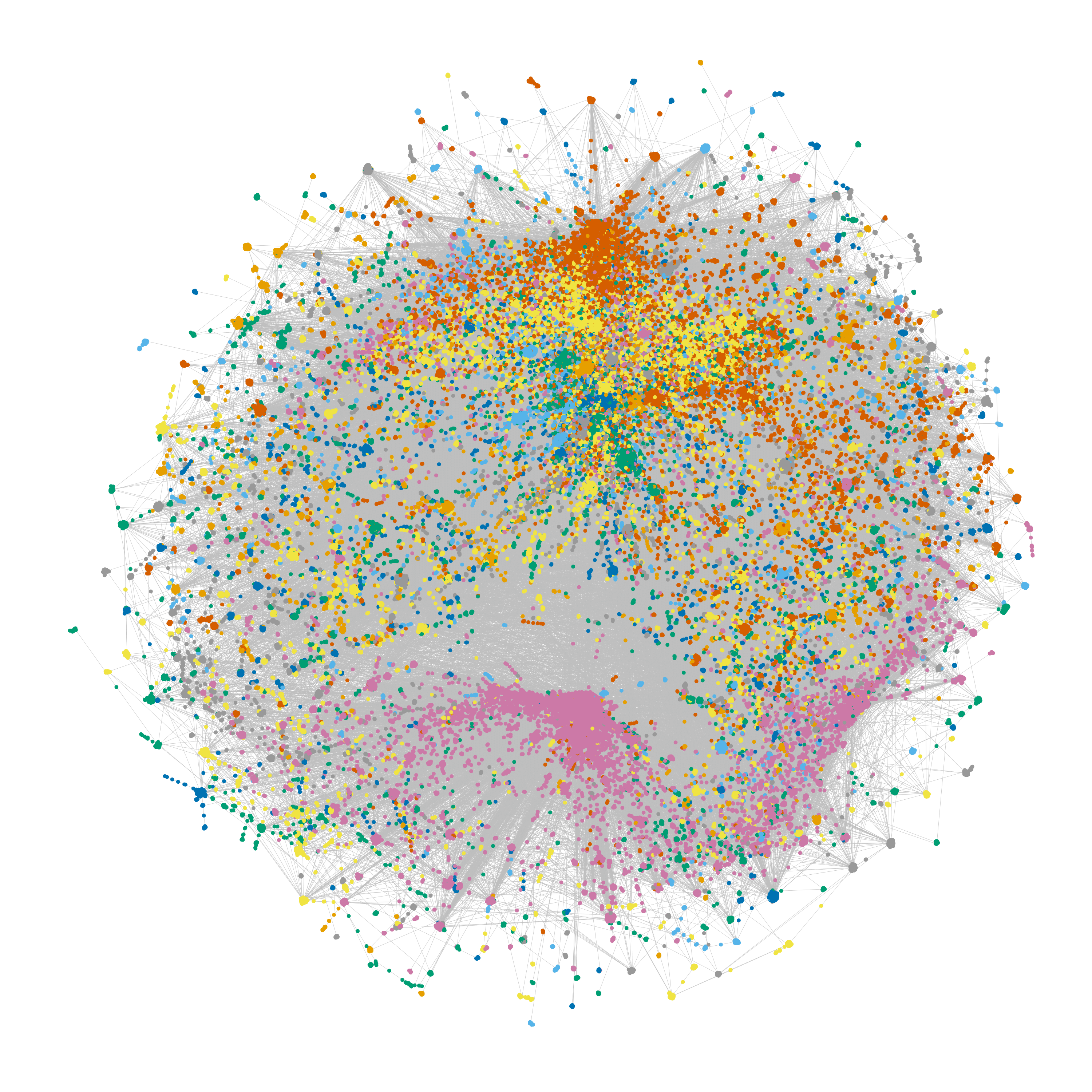
(a) 1st_Round network.

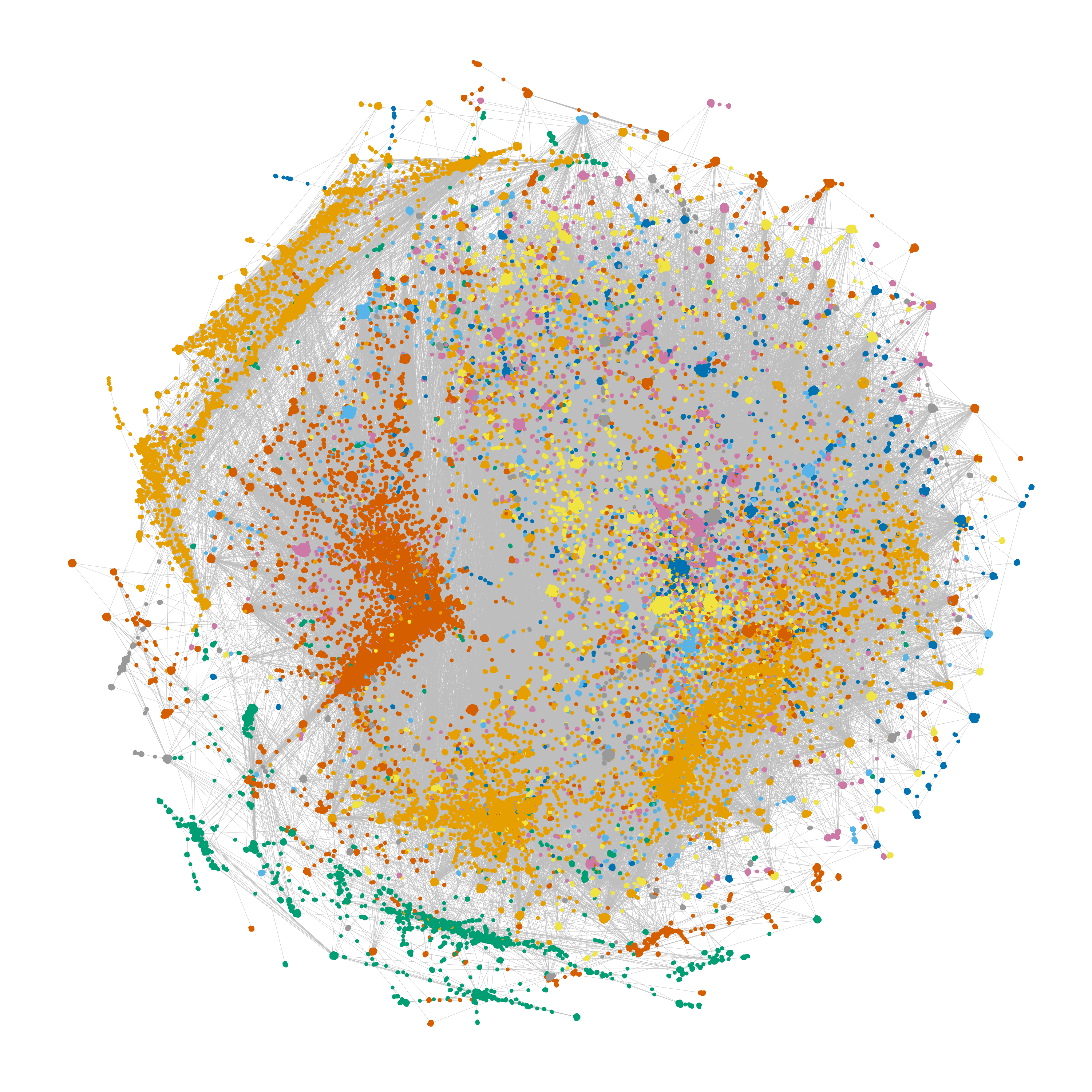
(b) 2nd_Round network.

Figure 2: Communities found by the Louvain method.

Next section presents the analysis performed to describe the topology and the community structure of the constructed networks.

6 Network Analysis

[Tedjamulia2005] suggested dividing the users of Twitter networks into categories according to their popularity and activity. In this paper, we have divided the users into 8 sets (categories) according to their popularity – number of mentions and retweets received by the user – and activity – number of mentions and retweets made by the user. The categories related to the popularity are called $PC1$, $PC2$, $PC3$ and $PCR$, whereas those regarding activity are $AC1$, $AC2$, $AC3$ and $ACR$. $PC1$ and $AC1$ contain the $0.1\%$ most popular and the $0.1\%$ most active users, respectively; $PC2$ and $AC2$ comprise the $1\%$ most popular users not in $PC1$ and the $1\%$ most active users $AC1$, respectively; $PC3$ and $AC3$ have the $10\%$ most popular users that are neither in $PC1$ nor in $PC2$ and the $10\%$ most active users that are neither in $AC1$ nor in $AC2$; and $PCR$ and $ACR$ comprise as the $90\%$ least popular and the $90\%$ least active users, respectively.

According to these sets of users, the $1\%$ most popular and active users are those from $PC1\cup PC2$ and $AC1\cup AC2$, respectively. The $10\%$ most popular and active users are those that belong to $PC1\cup PC2\cup PC3$ and $AC1\cup AC2\cup AC3$, respectively.

Now, consider the division of tweets into sets (categories) according to their popularity regarding only the number of retweets they received: $TC1,TC2,TC3$ and $TCR$ are the categories of tweets and are respectively ranked as the $0.1\%$ most popular tweets, $1\%$ most popular tweets not in $TC1$, $10\%$ most popular tweets not in $TC1$ nor in $TC2$ and $90\%$ least popular tweets.

The following sections show the analysis of the constructed networks with respect to the popularity and activity of their users, tweets and communities. Moreover, they also show the evolution of the topologies of the networks along time. The classification of users into communities and the spread of viral tweets is also discussed. In particular, the results of the largest network 1st_Round are further investigated.

6.1 Users’ Popularity and Activity

This section presents the analysis of the proposed networks with respect to the distribution of their degrees in order to describe the popularity and activity of the users and their influence on the constructed networks. The section investigates the 1st_Round network more thoroughly whereas the other networks are loosely discussed.

The popularity of a user is measured by the total number of mentions and retweets that they receive. A user’s activity is defined by the number of mentions and retweets they make. According to the definition of arcs presented in Section Extracted Networks, the in- and out-degrees of a vertex represent, respectively, the activity and the popularity of the user that the vertex refers to.

Large social networks are usually scale-free. In particular, on Twitter-based networks, the most visible users are the nodes with the highest degrees. To analyze the topology of the constructed networks, Figures 3(b) and 3(a) exhibit histograms with the out- and in-degree frequencies of 1st_Round.

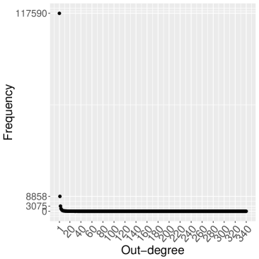
(a) Out-degree distribution.

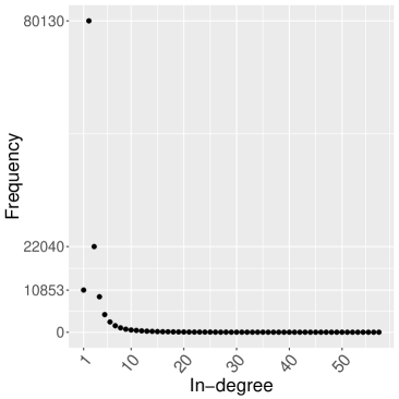
(b) In-degree distribution.

Figure 3: Histograms of the out- and in-degree distributions of 1st_Round.

As can be noted in Figure 3, the distribution of the node degrees follows a power law. The power law degree distribution of the vertices corroborates with the observation that a few users are more active or visible in social networks.

[Bruns2013] stated that a minority of users is very active or popular in a Twitter network. In the 1st_Round network, users from $ACR,AC3,AC2$ and $AC1$ were responsible for, respectively, $61.08\%,28.54\%,8.28\%$ and $2.11\%$ of the total number of tweets. Users from $PCR,PC3,PC2$ and $PC1$ received, respectively, $1.88\%,15.75\%,29.62\%$ and $52.75\%$ of the total number of retweets. As a consequence, on the one hand the 90% least active users ($ACR$) were responsible for posting most of the mentions and retweets. On the other, the top $1\%$ most popular users ($PC1\cup PC2$) received most of the mentions and retweets.

Also, $89.77\%$ of users from $PCR$ were among the $90\%$ least active users, i.e., they belonged to $ACR$. A total of $7.01\%$ of users who ranked between the $1\%$ and the $10\%$ most popular users (in $PC3$) are also between the $1\%$ and $10\%$ most active ones (in $AC3$). Only $1.18\%$ of the top $1\%$ most popular users (in $PC1\cup PC2$) belong to the top $1\%$ most active users (in $AC1\cup AC2$). None of the 0.1% most popular users, i.e. in $PC1$, is among the top 0.1% most active users, i.e. in $AC1$. Since users from $PC1\cup PC2$ are responsible for $82.37\%$ of the tweets, it is possible to conclude that the most popular users are not necessarily the most active ones. This conclusion makes sense since the top $0.1\%$ most popular users are news organizations or public figures, such as, for example, politicians and journalists, who get more retweets than effectively post tweets on Twitter. The most popular users, therein, must effectively post popular tweets that receive most of the retweets and mentions.

Table 4 exhibits the percentage of the tweets posted by users from each popularity category. As can be seen in the table, the higher the popularity of the tweets, the higher the popularity of the users who posted them.

Table 4: Percentage of tweets posted by users from each popularity category for network 1st_Round.

		Users
		$PCR$	$PC3$	$PC2$	$PC1$
Tweets	$TCR$	0.26%	94.88%	4.34%	0.52%
	$TC3$	0%	27.96%	67.68%	4.37%
	$TC2$	0%	0%	44.16%	55.84%
	$TC1$	0%	0%	0%	100%

Table 5 shows an analysis of the activity and popularity of users in the networks introduced in this paper. In this table, column “Network” identifies the network under analysis; column “Contribution to tweets posted” presents the percentage of mentions and retweets sent by the users from activity categories; column “Contribution to retweets” shows the percentage of mentions and retweets received by the users from popularity categories; column “Popular users ranked as active” presents the percentage of users ranked into popularity categories who are also in activity categories; and column “Popular tweets posted by users” presents the percentage of the 90% least and 10% most popular tweets posted by the 90% and 10% most popular users, respectively.

Table 5: Analysis of popularity and activity of users in the proposed networks.

Network	Contribution to				Contribution to				Popular users			Popular tweets
	tweets posted				retweets or mentions				ranked as actives			posted by users
	$ACR$	$AC3$	$AC2$	$AC1$	$PCR$	$PC3$	$PC2$	$PC1$	$ACR$	$AC3$	$AC1\cup AC2$	$PCR$	$PC1\cup PC2\cup$
									in	in	in	in	$PC3$ in $TC1\cup$
									$PCR$	$PC3$	$PC1\cup PC2$	$TCR$	$TC2\cup TC3$
Politicians	53.24%	30.66%	11.03%	5.07%	5.11%	29.15%	36.88%	28.87%	91.04%	15.08%	5.56%	44.59%	100%
Lula	44.73%	35.61%	14.05%	5.62%	2.91%	25.86%	39.14%	32.09%	91.11%	15.03%	5.97%	90.34%	9.63%
Bolsonaro	58.65%	29.89%	6.8%	4.65%	22.37%	34.37%	18.62%	24.64%	89.94%	5.13%	10%	85.62%	16.67%
LavaJato	44.63%	35.76%	13.99%	5.61%	3.2%	26.86%	38.54%	31.39%	91.11%	15.23%	7.04%	91.29%	11.58%
1st_Round	61.08%	28.54%	8.28%	2.11%	1.88%	15.75%	29.62%	52.75%	89.77%	7.01%	1.18%	27.09%	100%
2nd_Round	61.53%	28.03%	8.31%	2.14%	0.87%	17.61%	35.43%	46.09%	89.5%	4.73%	1.39%	14.49%	100%

The values in Table 5 corroborate with the findings on network 1st_Round: the 90% least active users ($PCR$) are responsible for posting most of the mentions and retweets; the top $1\%$ most popular users receive most of the mentions and retweets; the top $1\%$ most popular users are mostly not ranked in the top $1\%$ most active; and less than $11\%$ of the $1\%$ to $10\%$ most popular users ($PC3$) are also ranked as the $1\%$ to $10\%$ most active users ($AC3$).

However, for all the networks but Politicians, 1st_Round and 2nd_Round, the percentage of the top $10\%$ most popular users ($PC1\cup PC2\cup PC3$) who posted the top $10\%$ most popular tweets ($TC1\cup TC2\cup TC3$) ranged from $9.28\%$ to $16.67\%$. According to this result, the tweets that received most of the retweets were not necessarily posted by the most popular users. The users’ popularity might therefore be due to: (i) retweets received from a plethora of tweets; or (ii) mentions received from other users.

In the next section, like [Sluban2015], we shall analyze the influence of the most popular users on the communities.

6.2 Influence of the Most Popular Users and Tweets

The popularity of a community is defined by the sum of the popularity of its users, that is, the total out-degree of the vertices that belong to the community.

Figure 4 presents the percentage of users from each popularity category in the communities of network 1st_Round. Each community is described on the x-axis according to their size. Figure 5 shows the contribution of the users from each popularity category, in percentage, to the total popularity of the communities found by Louvain in network 1st_Round. Again, the x-axis indicates the size of the communities, which is the number of vertices in a community.

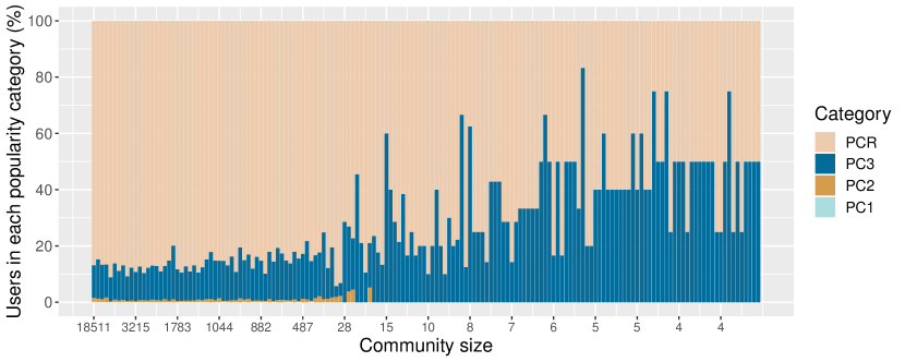
Figure 4: Percentage of users in the communities found by Louvain method in network 1st_Round.

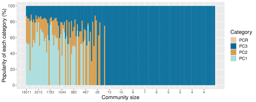
Figure 5: Contribution of each popularity category, in percentage, to the popularity of the communities found by Louvain method in network 1st_Round.

Although in smaller number, the top $0.1\%$ most popular users ($PC1$) are responsible for the majority of the community’s popularity for most of the communities with more than 28 vertices. Users from $PC2$ have also significantly contributed to the popularity of the communities. As expected, although the $90\%$ least popular users ($PCR$) are the majority of users in the communities, they do not contribute to the popularity of the communities.

The social influence on a community is the percentage of the retweets or mentions its users receive made by users from other communities [Sluban2015]. Figures 7 and 7 summarize the influence exerted by, respectively, users and tweets from each popularity category in the communities.

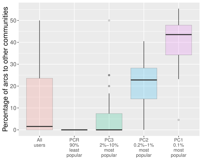
Figure 6: Influence exerted by users of the communities in network 1st_Round.

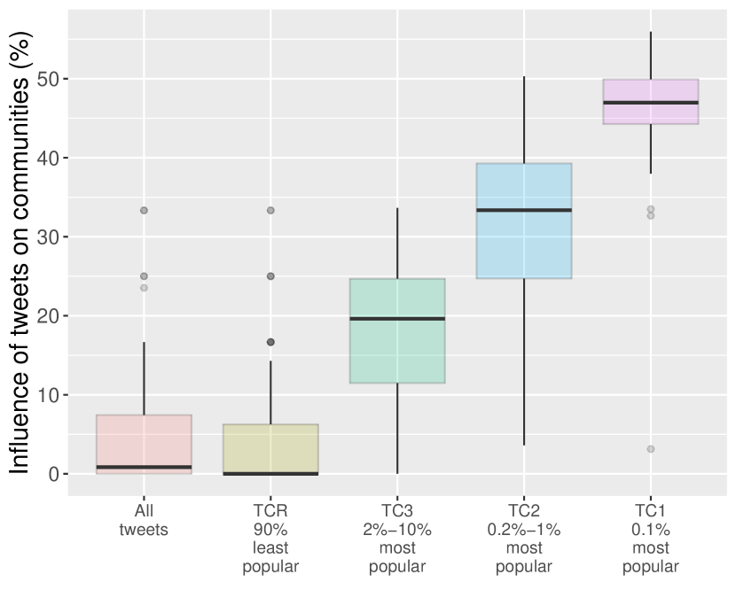
Figure 7: Influence exerted by tweets of the communities in network 1st_Round.

The $90\%$ least popular users have an average influence very close to $0$, meaning that most of the retweets and mentions they receive are made by users within their community. Users from $PC2$ and $PC1$ have higher social influence on their communities than $PC3$. A similar conclusion can be drawn on the influence of the most retweeted tweets on communities. The social influence concerning tweets from $TC3$, $TC2$ and $TC1$ are substantially higher than of users from $TCR$, which suggests that the $10\%$ most retweeted tweets are indeed good candidates to be viral tweets.

We classify a tweet as viral if its virality is greater than the threshold $0.25$, that is, at least $25\%$ of the retweet it receives is from communities other than the one it originated from. Figure 8 exhibits the percentage of viral tweets in the communities of network 1st_Round regarding each tweet popularity category. According to this figure, the higher the popularity of the tweets, the higher their chance of being viral. In particular, all of the $0.1\%$ most popular tweets ($TC1$) are viral.

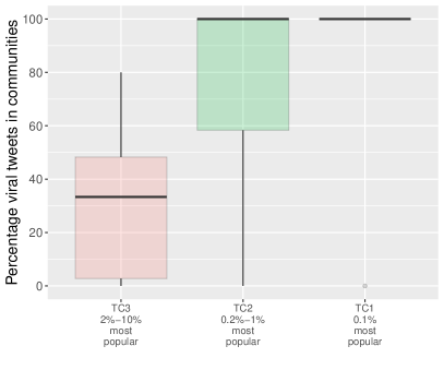
Figure 8: Percentage of viral tweets in the communities of network 1st_Round.

Table 6 presents a brief analysis of the communities found by the Louvain method in the networks introduced in this paper. In this table, columns “Number of users in communities (%)” and “Popularity of users in communities (%)” exhibit the percentage of users from each popularity category and their popularity, respectively, in the communities. Column “Viral tweets” shows the percentage of the $10\%$ most popular tweets that are viral. The columns marked as “avg” and “std” exhibit, respectively, the average and standard deviations of the aforementioned values.

Table 6: Analysis of the communities found by Louvain for the constructed networks.

Network	Number of users in communities (%)								Popularity of users in communities (%)								Viral		Virality of
	$PCR$		$PC3$		$PC2$		$PC1$		$PCR$		$PC3$		$PC2$		$PC1$		tweets (%)		tweets (%)
	avg	std	avg	std	avg	std	avg	std	avg	std	avg	std	avg	std	avg	std	avg	std	avg	std
Politicians	88.85	15.46	10.75	15.39	0.38	1.09	0.02	0.07	42.4	46.81	65.29	35.43	56.93	27.27	55.85	27.32	32.78	31.41	10.14	10.78
Lula	78.62	18.1	20.95	18.27	0.41	0.72	0.03	0.07	11.6	22.96	65.69	34.08	53.07	24.22	54.05	29.54	100	0	91.11	11.36
Bolsonaro	87.58	9.16	11.67	9.7	0.64	1.12	0.11	0.37	31.45	19.94	49.03	25.99	62.2	26.66	75.37	16.26	97.44	9.25	87.35	19.01
LavaJato	80.2	14.16	19.45	14.31	0.33	0.68	0.02	0.07	17.77	29.22	67.76	32.26	50.2	25.04	51.54	31.1	100	0	92.55	9.36
1st_Round	71.47	17.31	28.1	17.63	0.4	0.76	0.03	0.05	0	0	70.43	37.59	36.07	22.88	58.56	13.1	55.54	40.09	4.6	6.33
2nd_Round	74.72	15.6	24.91	15.93	0.34	0.66	0.03	0.05	0	0	72.7	37.87	41.14	25.69	56.4	21.42	47.24	41.86	7.99	9.98

On the one hand, the results of “Number of users in communities (%)” and “Popularity of users in communities (%)” presented in Table 6 confirm the preceding analysis of network 1st_Round: the most popular users are responsible for most of the popularity of the communities. On the other hand, all or almost all the $10\%$ most popular tweets are viral on the remaining networks.

Except for the Politicians, 1st_Round and 2nd_Round networks, tweets had viralities higher than $83.75\%$. The average virality of tweets from Politicians, 1st_Round and 2nd_Round networks, on the other hand, were lower than $10.14\%$.

Next section presents an analysis of the growing patterns in network 1st_Round.

6.3 Temporal Analysis of 1st_Round Network

To understand how the popularity and activity of users from network 1st_Round evolves along time, we took snapshots of the network at every 5000 tweets. Each snapshot represents the network constructed from the tweets posted up to that time. Figure 10 presents the average out-degree, that is, the number of retweets received from users from each popularity set with regard to the snapshots. Figure 10 presents the average in-degree, that is, the number of mentions and retweets made by users from each activity set with regard to the snapshots.

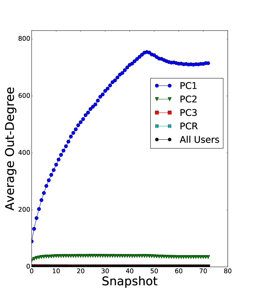
Figure 9: Average out-degree of users in popularity categories along time windows.

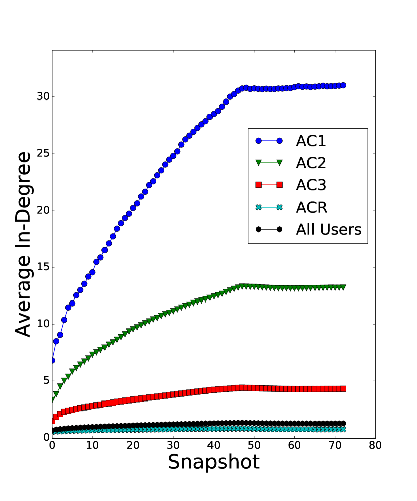
Figure 10: Average in-degree of users in activity categories along time windows.

The top $0.1\%$ most popular users ($PC1$) received an increasing number of retweets along time, as shown by their augmenting average out-degree. This observation corroborates with the remark that new vertices are more likely to connect with the existing vertices with the highest degrees in scale-free networks.

Figure 11 presents the evolution of network 1st_Round along time. In each snapshot, the following are considered: the total number of communities in the network obtained by the Louvain method, the average community size, the total number of arcs and nodes, the number of new tweets and the total number of different tweets in the network. As shown in Table 2, the network 1st_Round has 135865 nodes and 242679 arcs. It is possible to notice in Figure 11 that the number of new tweets that appear in the network at each snapshot is nearly constant. However, at snapshot 48, the number of new tweets drops significantly and then immediately starts to raise again.

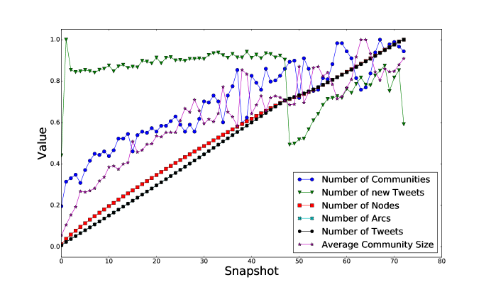
Figure 11: Evolution of network Politicians over time.

On average, 15% of the new arcs that appear in the network in a given snapshot represent retweets and mentions of new tweets. The other 85% of the new arcs represent new retweets and mentions of tweets already in the network in previous snapshots. The number of arcs created from a tweet decreases rapidly over time. In Figure 10 it is possible to note that the popularity of users from ${PC1}$ ceases to increase just in snapshot 48, where the number of new tweets is smaller.

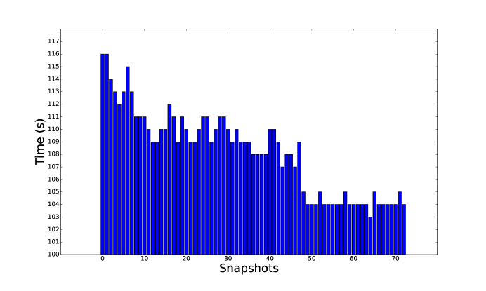
Figure 12: Duration of each snapshot in seconds.

Figure 12 shows the duration (in seconds) of each snapshot. The average duration of each snapshot was 108 seconds, which means that 5000 tweets were collected at every 108 seconds. The average duration of snapshots before and after snapshot 48 was, respectively, 110 and 104 seconds. Snapshot 48 was collected upon the disclosure of the results of the first round of the elections at 19:00:00 (Brasília Time (BRT)), while snapshot 49 was collected from 19:00:38 to 19:02:23 (Brasília Time (BRT)). On the one hand, the average duration of the snapshots obtained after the release of the first round of results decreased. That is, the 5000 tweets collected in each snapshot were obtained in a shorter time window, which meant that Twitter users were more active. On the other hand, the number of new tweets appearing in snapshot 49 is smaller than in previous snapshots. This possibly means that, during the disclosure of the election results, users created fewer new tweets and interacted more with previously posted tweets. However, the rate of new tweets soars after snapshot 48, whose content was probably about the released results.

7 Context and Sentiment of the Communities in Relation to the Elections

The output of a community detection algorithm provides a straightforward classification of users into communities. Tweets can be classified according to the communities of the users who posted them. In this section the context of the communities and their sentiments in relation to the words in the tweets of networks 1st_Round and 2nd_Round are studied.

Prior to the sentiment analysis, we first selected the words which were used at least 10 times in the communities with a minimum of 1000 vertices. Then, we translated all the words into English. Finally, we employed the R library sentimentr [sentimentr] to analyse the sentiment related to the selected words in each community. Each word is associated with a score in the range [-1,1], where -1 and 1 indicate the most negative and positive sentiments, respectively.

Figures 13(a) and 13(b) illustrate word clouds with the most frequent words in the tweets from networks 1st_Round and 2nd_Round. The word cloud in Figure 13(a) shows that the names of the three most voted candidates in the first round of the elections were also amongst the most used words. This word cloud also shows the words “segundo” and “turno”, which mean “second” and “round” in English, respectively, suggesting interest in the second round during the first round of the elections. The word cloud in Figure 13(b) shows the name of the two candidates who ran in the second round of the elections.

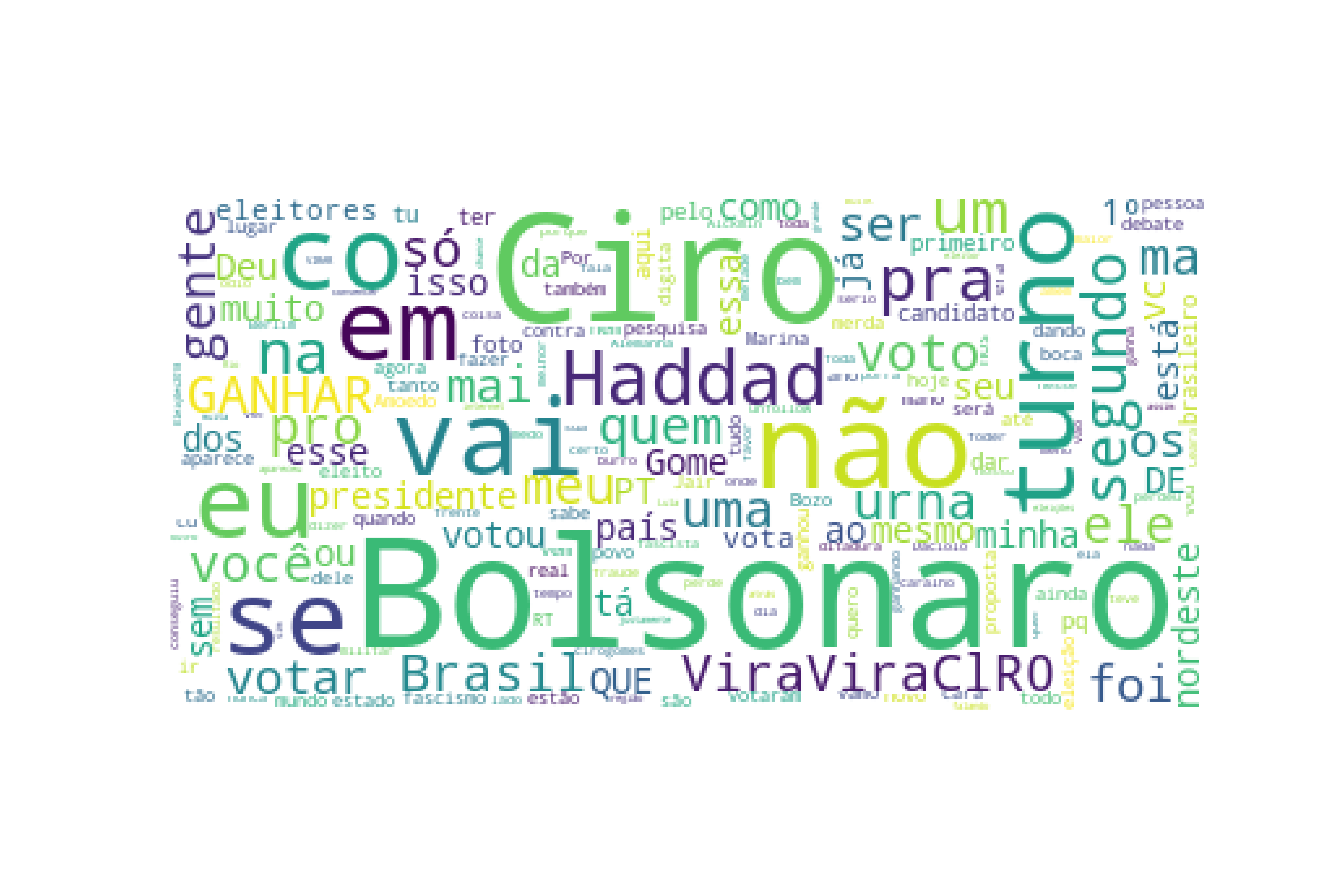
(a) Word Cloud for network 1st_Round.

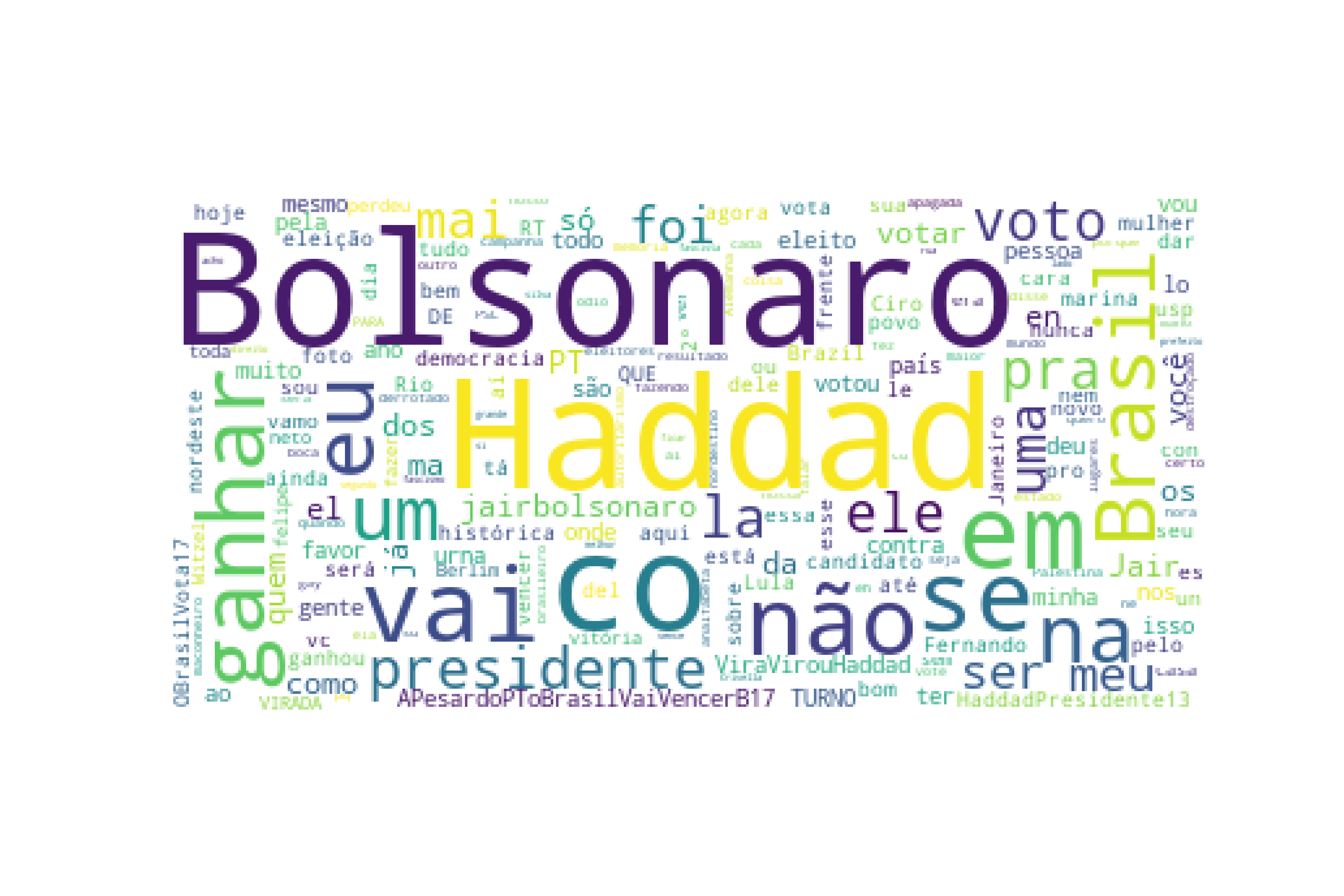
(b) Word Cloud for network 2nd_Round.

Figure 13: Word clouds with the most frequent words.

Figures 14(a) and 14(b) show the sentiment of the most common words in the tweets from networks 1st_Round and 2nd_Round. The x-axis in the figures presents the size of the communities, i.e., their number of vertices. The y-axis shows the sentiment of the words. The center of the circumferences indicates the sentiment of the words whereas their diameter indicates the frequency of the data collected: higher diameters indicate words used more often. These figures show that the sentiment and frequencies of the words in the data collected regarding the first and second rounds of the elections are similar. The higher the size of the community, the higher the frequency of the words. Moreover, although the number of words associated with negative and positive sentiments is similar, the words associated with positive sentiments appear more often.

(a) Network 1st_Round.

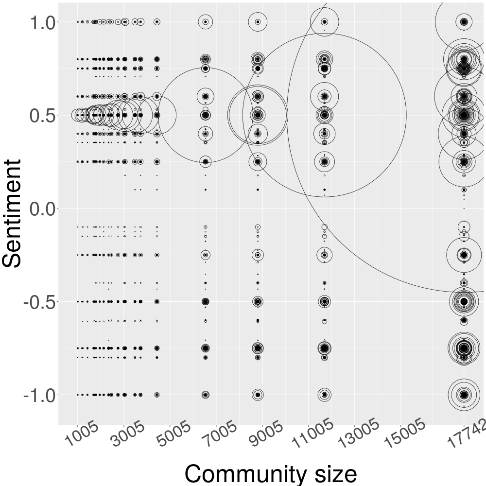
(b) Network 2nd_Round.

Figure 14: Sentiments associated with the most common words on the communities.

Based on the observation that the words associated with positive sentiments are more frequent, the sentiment of the words that appear more times in the tweets should weigh more in a general sentiment score. Thereby, we calculate the average sentiment score of each community as the sum of the sentiments associated with each word multiplied by its frequency in the community.

Figures 15 and 16 present the average sentiment score of the communities with at least 1000 vertices. In these figures, the vertices belonging to the community found using the Louvain method are collapsed into supernodes and the edges between them represent the existence of arcs between its vertices. The larger the size of a supernode, the higher the number of vertices in the community. Similarly, the thickness of the edges is proportional to the amount of arcs between the communities. Additionally, for the 7 largest communities, these figures also show the three negative and positive words associated with the highest and lowest scores, respectively. The word in Portuguese is presented next to a green or red square whose color intensity is proportional to the sentiment score and the number of times the word was used in the community.

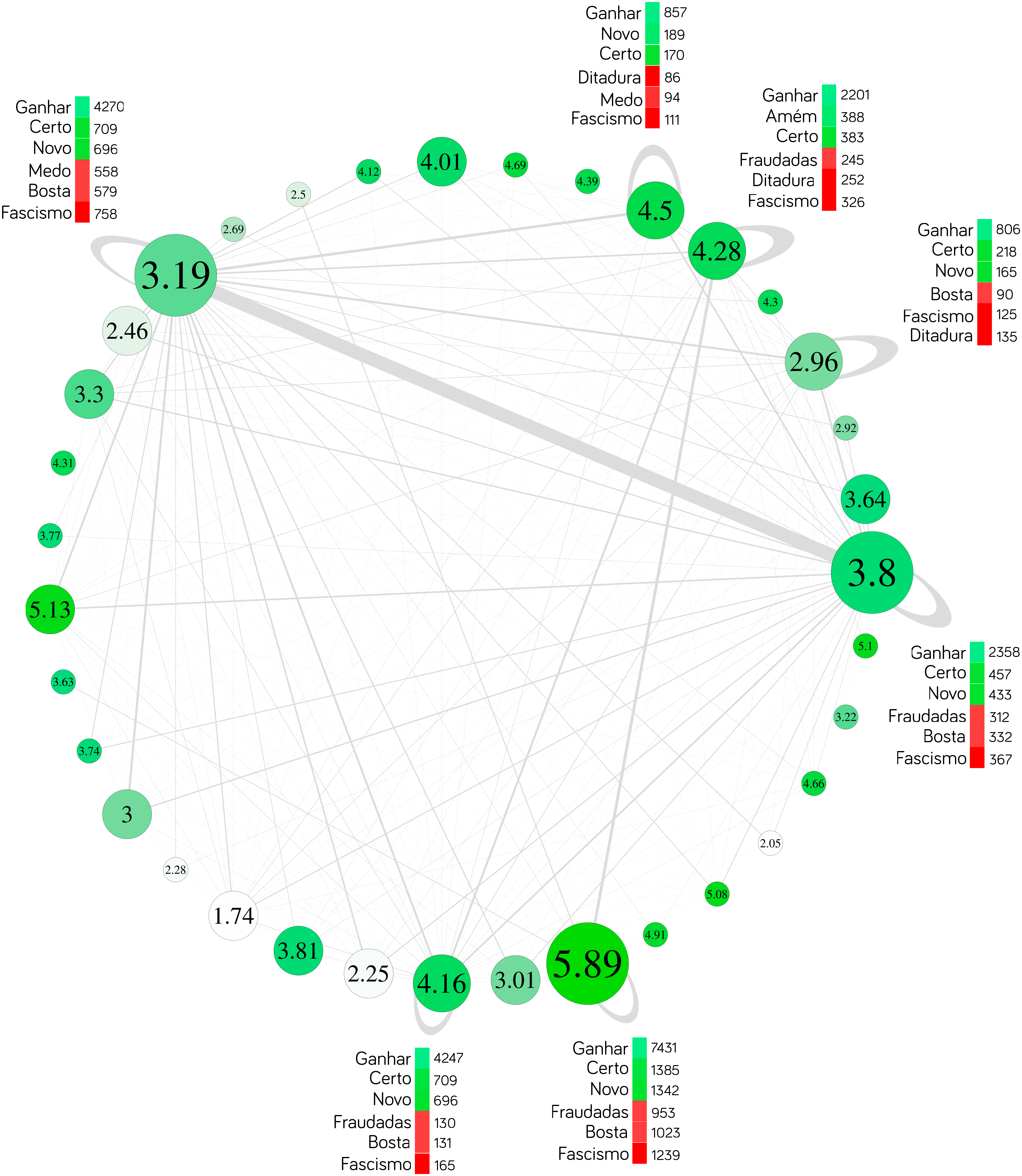
Figure 15: Average sentiment score and words associated with the highest positive and negative scores in communities considering network 1st_Round.

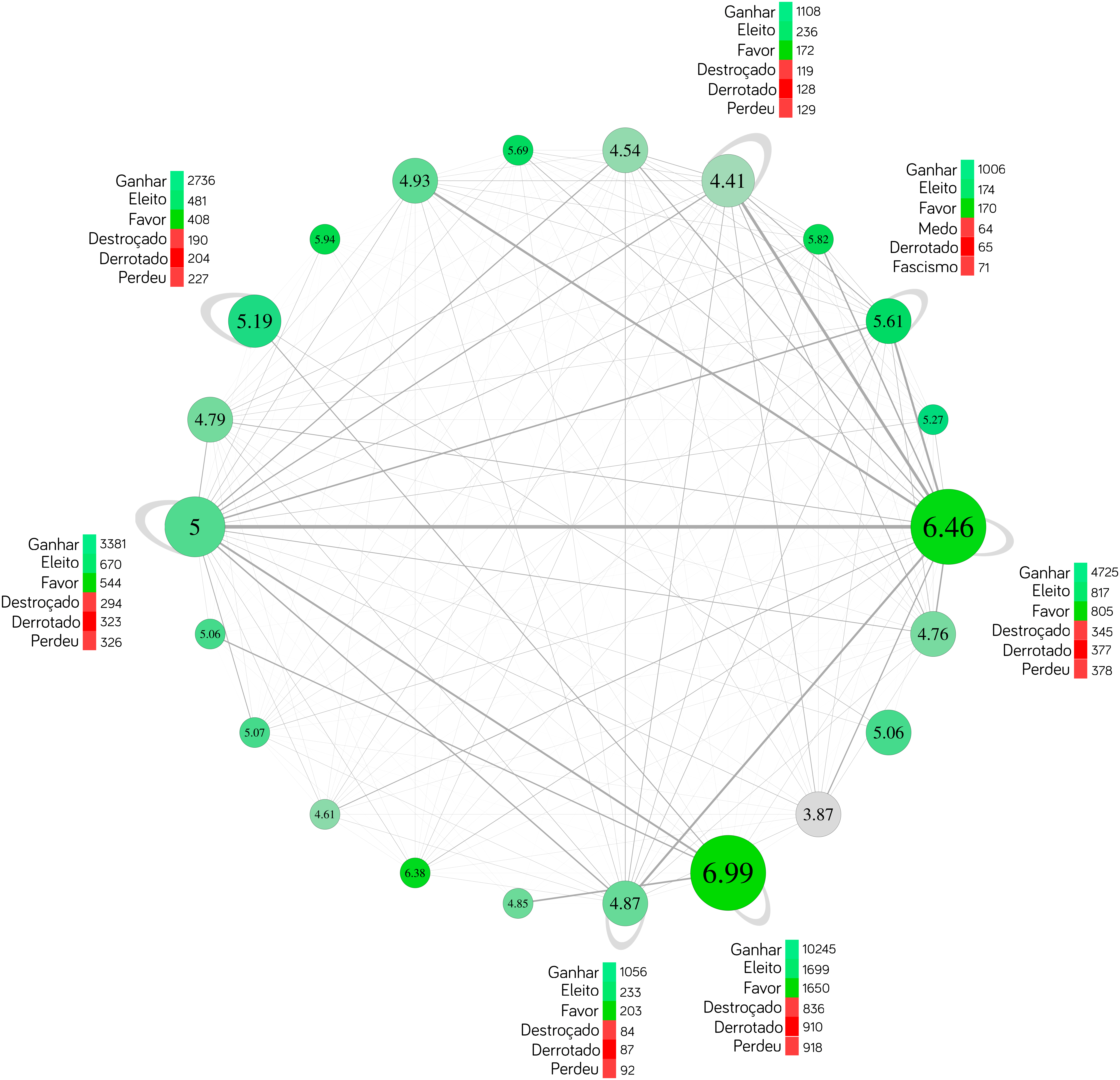
Figure 16: Average sentiment score and words associated with the highest positive and negative scores in communities considering network 2nd_Round.

The scores presented in Figures 15 and 16 show that, on average, the sentiment associated with the words in the communities was positive. However, this result is due to the higher frequency of positive words. These words are also amongst the most frequent words exhibited in the word clouds of Figures 13(a) and 13(b).

Moreover, the words associated with the highest scores are the same in all the communities in both Figures 15 and 16. These words occur in tweets classified as $TC1$, i.e, the $0.1\%$ most popular tweets, which according to Figure 8, are viral tweets. This observation corroborates with [Wang2013], who state that viral tweets spread across the communities.

8 Final Remarks and Future Works

This paper presents a thorough analysis of the structure and topology of networks constructed from political discussions on Twitter and, in particular, discusses networks composed by tweets expressing reactions to the 2018 Brazilian presidential elections.

These networks are scale-free and a minority of their users are responsible for receiving most “retweets” and “mentions”, while effectively posting few tweets. The evolution of the networks along time showed that new users are more likely to interact with the most popular users. We verified that the study by [Weng2013] on the spreading patterns of hashtags was valid for the spreading of retweets on a political network regarding the 2018 Brazilian presidential elections: most tweets were retweeted by users from within the community of the user who originally posted the tweet but the minority of tweets is retweeted from several different communities and spread like viruses.

The most popular users, although in smaller number, dictate the popularity of the communities and the higher their popularity, the greater their influence on other communities. These users are also responsible for posting viral tweets.

Moreover, we studied the sentiment related to the most frequent words in the tweets with content about the 2018 Brazilian presidential elections and discovered that, overall, words associated with positive sentiments are predominant. The words that contribute most to the positive sentiment of the communities are the same and appear in viral tweets.

As a future application of this work, we intend to further investigate and classify tweets from larger databases, in particular, reactions to the 2018 Truckers’ Strike and to the 2018 World Cup. To deal with the large scale networks, we plan to design distributed algorithms. In addition, the study of the evolution of the networks with respect to spreading patterns of the tweets might help us to understand how communities are formed and the proliferation of tweets along time. Finally, the observation that viral tweets do not affect the community structure of the networks and that non-viral tweets get trapped within the communities could be explored through community detection algorithms in order to provide better communities.