Kinematic detections of protoplanets: a Doppler-flip in the disk of HD 100546.

Abstract

Protoplanets and circumplanetary disks are rather elusive in their thermal IR emission. Yet they are cornerstone to the most popular interpretations for the protoplanetary disks structures observed in the gas and dust density fields, even though alternative theories exist. The gaseous velocity field should also bear the imprint of planet-disk interactions, with non-Keplerian fine structure in the molecular line channel maps. Such kinks or wiggles are affected by the optical depth structure and synthesis imaging limitations, but their detail could in principle be connected to the perturber by comparison with hydrodynamical simulations. These predictions appear to have been observed in HD 163296 and HD 97048, where the most conspicuous wiggles are interpreted in terms of embedded planets. The velocity centroid maps may allow for more robust indirect detections of embedded planets. The non-Keplerian velocity along the planetary wakes undergoes an abrupt sign reversal across the protoplanet. After subtraction of the disk rotation curve, the location of the perturber should be identifiable as a Doppler-flip in velocity centroid maps. Here we improve our rotation curves in an extension to disks with intermediate inclinations, which we apply to deep and fine angular resolution CO isotopologue datasets. Trials in HD 163296 and in HD 97048 yield non-detections. However, in HD 100546 we pick-up a conspicuous Doppler-flip, an important part of which is likely due to radial flows. Its coincidence with a fine ridge crossing an annular groove inside the continuum ring suggests a complex dynamical scenario, in which the putative protoplanet might have recently undergone pebble accretion.

1 Introduction

Direct detections of protoplanets and their circum-planetary accretion disks (CPDs) are difficult in their thermal IR emission. Only one example appears to hold scrutiny (i.e. PDS70b, Keppler et al., 2018). Yet most models for the structures observed in protoplanetary disks involve planet-disk interactions: giant planets evacuate radial gaps, launch spiral arms, and trigger crescent-shaped pile-ups of mm-grains. The gas and dust density fields are thus appealing proxies of the location and mass of embedded bodies (e.g. Dong & Fung, 2017). The planetary origin of such density structures is debated, however, as exemplified by the alternative scenarios in HL Tau and TW Hya (e.g. Dong et al., 2018, and references therein).

Molecular-line kinematics provide an alternative approach to the identification of protoplanets, as the gaseous velocity field also bears the imprint of planet-disk interactions. We have linked embedded planets with wiggle-shaped deviations from sub-Keplerian rotation in channel maps (Perez et al., 2015). However, such wiggles are ubiquitous in channel maps and can also be due to noise or systematics from synthesis imaging, or from structure in the underlying gas and dust optical depth. Hydrodynamical simulations are required to infer the location of embedded planets from the observed channel map wiggles. These predictions appear to match the data in HD 163296 and in HD 97048, where the most conspicuous wiggles are interpreted in terms of the location and mass of the perturber (Pinte et al., 2018b, 2019). In a companion Letter (Perez et al., 2019, ApJL, submitted - hereafter paper I) we report on another conspicuous wiggle in HD 100546.

The location of the perturbing body should be identifiable in velocity centroid maps $v_{\circ}(\vec{x})=\langle vI\rangle=\int dvvI_{v}/\int I_{v}dv$, where $I_{v}(\vec{x})$ are the molecular line channel maps as a function of line-of-sight velocity $v$. In hydrodynamical simulations, and typically for the disk midplane, the radial and azimuthal velocity deviations after subtraction of the sub-Keplerian background flow, are highest along the planetary wakes, and abruptly change sign at the location of the planet (e.g. see Fig. 1 in Pérez et al., 2018). At non-zero inclination this velocity reversal should be observable as a Doppler-flip, provided that the azimuthally symmetric background is adequately subtracted. Away from the midplane, the planetary wakes have significant vertical and radial motion which increases with altitude (Zhu et al., 2015). Most of the material interacting with a giant planet falls onto the midplane from high latitudes via meridional flows (Morbidelli et al., 2014; Dong et al., 2019), including both radial and vertical velocity components. We thus designed a technique to filter the velocity centroid image and pin-point the location of the perturber, yielding favorable predictions for 5  to 10 M_jup bodies given current ALMA capabilities (Pérez et al., 2018).

The rotation curve of a disk, $\tilde{v}_{\phi}(r)=\int dzd\phi\,\rho v_{\phi}/\int dzd\phi\,\rho$, in cylindrical coordinates, represents the mass-averaged tangential velocity in the plane of the disk as a function of radius. Among other uses in astrophysics, $\tilde{v}_{\phi}(r)$ allows a measure of the stellar mass in circumstellar disks. Here we are interested in building the rotation curve of protoplanetary disks with the goal of detecting deviations from azimuthal symmetry. We improve our method by taking azimuthal averages on conical surfaces (Section 2), and report applications to observations (Sec. 3) with emphasis on HD 100546, where we pick-up a conspicuous Doppler-flip.

2 Rotation curves and orientation of flared disks from velocity centroid maps

Dynamical stellar masses and measurements of $\tilde{v}_{\phi}(r)$ are usually obtained with forward-modeling of molecular-line data. Parametric radiative transfer (RT) modeling, with prescribed $\tilde{v}_{\phi}(r)$, can be compared against observations of $I_{v}(\vec{x})$ (e.g. Czekala et al., 2015). Such dynamical masses are indeed within 5–10% of independent estimates for close binaries (Rosenfeld et al., 2012; Czekala et al., 2015, 2016). However, the inferred $\tilde{v}_{\phi}(r)$ may not necessarily follow the details of the rotation curve, for instance because of the vertical velocity structure. Rotation curves have recently been measured empirically by noting that the tangential velocity component and height over the disk midplane can be solved for at two specific locations in the sky (for each of the near and far sides of the disk), given knowledge of disk orientation (Pinte et al., 2018a). This local datum for the disk height (or aspect radio $h$) has been extrapolated to deproject a circle at constant height, and so fit for $\tilde{v}_{\phi}(r)$ (Teague et al., 2018). However, uncertainties in the local measurement of $h$, if it is itself noisy or perturbed by local deviations from axial symmetry, may propagate in the azimuthal averages when extrapolated to all azimuths.

Here the measurement of $\tilde{v}_{\phi}(r)$ is not driven by the dynamical mass, but rather by the deviations in $v_{\circ}(\vec{x})$ from the azimuthally-averaged background $\tilde{v}_{\circ}(\vec{x})=\tilde{v}_{\phi}(r)\cos(\phi)$, where the origin of $\phi$ coincides with the disk position angle (PA). We infer the bulk flow $\tilde{v}_{\circ}(\vec{x})$ directly from the observed velocity centroid map $v_{\circ}(\vec{x})$ and its uncertainty $\sigma^{2}_{\circ}(\vec{x})$, extracted from $I_{v}(\vec{x})$ using single-Gaussian fits to each line-of-sight spectrum (including a linear baseline for the continuum). Our main assumption is that the surface in the disk where the molecular line emission originates, i.e. the unit-opacity surface for optically thick lines, can be represented by a double cone. The free-parameters are reduced compared to forward-modeling, to only ($i$, PA, $h$). Disk flaring or radial variations in $h$ can be measured by binning the optimization in radius.

We consider three coordinates systems: $\mathcal{S}$ represents the sky frame, orientated with $(x,y,z)$ Cartesian coordinates, and where $y$ corresponds to North. $\mathcal{S}^{\prime}$ is also parallel to the sky, but its $y^{\prime}$ axis coincides with the disk PA. $\mathcal{S}^{\prime\prime}$ is the rotation of $\mathcal{S}^{\prime}$ about axis $\hat{y}^{\prime}$ by the inclination angle $i$, so that the $z^{\prime\prime}=0$ coincides with the disk midplane.

If all of the emission originates from the near side, we have a bijection between the line of sight $\vec{x}$, and the polar coordinate of its intersection with the surface of the cone representing the disk surface (defined as the surface of unit opacity). Given a point on the cone, with an opening angle $\psi=\arctan(h/r)$ above the disk midplane, and with cylindrical coordinates $r,\phi$ in $\mathcal{S}^{\prime\prime}$, we can compute the sky coordinates in $\mathcal{S}^{\prime}$ with the following conical transform $\vec{x}^{\prime}=\vec{f}_{\mathrm{PA},i,+\psi}(r,\phi)$ (see also Rosenfeld et al., 2013; Isella et al., 2018):

$$x^{\prime} = r\sin(\phi)/\cos(i)+(h-r\sin(\phi)\tan(i))\sin(i),$$ (1)

$$y^{\prime} = r\cos(\phi).$$ (2)

Here we use a linear law for $h(r)=\tan(\psi)r$. We can invert Eqs. 1 and 2 to obtain $(r,\phi)=\vec{f}^{-1}_{\mathrm{PA},i,+\psi}(x^{\prime},y^{\prime})$, by noting that $r$ is the root of:

$$\frac{y^{\prime\,2}}{r^{2}}+\frac{(x^{\prime}-h(r)\,\sin(i))^{2}}{r^{2}\cos^{2}(i)}=1.$$ (3)

Having solved for $r$ we obtain $\phi$ with

$$\cos(\phi)=y^{\prime}/r.$$ (4)

Given (PA, $i$, $\psi$) we resample the observed centroid $v_{\circ}(\vec{x})$ with the near-side conical transform $\vec{f}_{\mathrm{PA},i,+\psi}$:

$$v_{\circ+}(r,\phi)\equiv v_{\circ}\left(\vec{f}^{-1}_{\mathrm{PA},i,+\psi}(r,\phi)\right),$$ (5)

where the $+$ sign in $v_{\circ+}$ indicates the near-side conical surface (note that for $i>90\,$deg, the near side corresponds to $\psi<0$). We then take azimuthal averages,

$$v^{m}_{\circ+}(r_{l},\phi_{k})=\cos(\phi_{k})\tilde{v}_{\phi}(r_{l})+v_{s},$$ (6)

in discretized polar coordinates, by fitting for the rotation curve $\tilde{v}_{\phi}(r_{l})$ in a least-squares sense with

$$\chi^{2}_{\tilde{v}}=\sum_{k}w(r_{l},\phi_{k})(v_{\circ+}(r_{l},\phi_{k})-\tilde{v}_{\phi}(r_{l})\cos(\phi_{k})-v_{s})^{2},$$ (7)

with weights $w(r_{l},\phi_{k})=1/\sigma^{2}_{\circ}(r_{l},\phi_{k})$. When the systemic velocity $v_{s}$ is known,

$$\tilde{v}_{\phi}(r_{l})=\frac{\sum_{k}w(r_{l},\phi_{k})[v_{\circ+}(r_{l},\phi_{k})-v_{s}]\cos(\phi_{k})}{\sum_{k}w(r_{l},\phi_{k})\cos^{2}(\phi_{k})}.$$ (8)

If $v_{s}$ is not known we can fit for $v_{s}(r_{l})$ and $\tilde{v}_{\phi}(r_{l})$ simultaneously, fix $v_{s}$ to the median value and its uncertainty to its standard deviation, and then recompute $\tilde{v}_{\phi}(r_{l})$. We resample $v^{m}_{\circ+}(r,\phi)$ with $\vec{x}^{\prime}=\vec{f}_{\mathrm{PA},i,+\psi}(r,\phi)$ and rotate back to $\mathcal{S}$ to obtain the sky map for the azimuthally-averaged centroid, $v^{m}_{\circ+}(\vec{x})$.

We optimize $i$, PA and $\psi$ so as to maximize the log-likelihood function, $-0.5\chi^{2}$, with

$$\chi^{2}=\frac{1}{N_{\mathrm{corr}}}\sum_{l=l1}^{l2}\sum_{k=0}^{N_{\phi}}w(r_{l},\phi_{k})(v_{\circ}(r_{l},\phi_{k})-v^{m}_{\circ+}(r_{l},\phi_{k}))^{2}.$$ (9)

The double sum extends over pixels in polar coordinates, within an interval in radius between $r_{1}$ and $r_{2}$, and over all azimuths. $N_{\mathrm{corr}}$ is the number of pixels in a beam, and approximately corrects $\chi^{2}$ for correlated datapoints.

Disk orientation may change with radius; even in the absence of warping the disk aspect ratio will vary. Passive disks are expected to be flared, but the height of the ¹²CO unit opacity surface will decrease with radius, so the trend in $\psi(r)$ is difficult to anticipate. We divide the full radial extension of the disk in $M$ (overlapping) radial bins $\{[r_{1j},r_{2j}]\}_{j=1}^{M}$, thus defining radial regions $\{\Theta_{j}(\vec{x}^{\prime})\}_{j=1}^{M}$, where $\Theta_{j}(\vec{x}^{\prime})=1$ if $r=f_{r}^{-1}(\vec{x}^{\prime})\in[r_{1j},r_{2j}]$, and $\Theta_{j}(\vec{x}^{\prime})=0$ otherwise. We take azimuthal averages of $v_{\circ}(\vec{x})$ in each region to produce $\{v^{m}_{j}(\vec{x})\}_{j=1}^{M}$. The azimuthally averaged centroid map combined over all regions is

$$v^{m}_{\circ R}(\vec{x})=\frac{\sum_{j=1}^{M}v^{m}_{\circ+}(\vec{x})\Theta_{j}(\vec{x})}{\sum_{j=1}^{M}\Theta_{j}(\vec{x})}.$$ (10)

In the applications below, the optimal orientation for the whole radial extension is $i_{\circ}$, PA_∘ and $\psi_{\circ}$, while the orientation profile is $i(r)$, PA$(r)$ and $\psi(r)$.

At finite inclinations parts of the far-side will contribute to $v_{\circ}(\vec{x})$, with a weight $\mu(\vec{x})$ that depends on the technique used to measure the velocity centroid. Including the far-side yielded small improvements in $\chi^{2}$, but complicates the interpretation of the velocity deviations, so we opted to present results with $\mu(\vec{x})\equiv 1$ only.

3 Applications

3.1 HD 100546

In paper I we report on a conspicuous wiggle in ¹²CO(2-1) ALMA observations of HD 100546. We apply our velocity filter to the velocity centroid map extracted from these data. Fig. 1 summarizes the result of an optimization of disk orientation and rotation curve. The difference between observations and azimuthally-averaged model, $v_{\circ}-v_{\circ}^{m}$, in Fig. 1 d shows a Doppler-flip related to that wiggle, with a total amplitude of 2.6 km s^-1 where the rotation curve is $\tilde{v}_{\phi}\sim$6 km s^-1. We can also identify spiral arms in $v_{\circ}-v_{\circ}^{m}$, some of which have previously been detected in the IR (Boccaletti et al., 2013; Garufi et al., 2016).

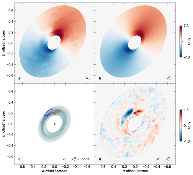
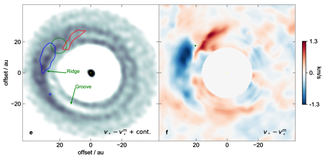
Figure 1: Doppler-flip in HD 100546. a: $v_{\circ}$, observed ¹²CO(2-1) line centroid (paper I, $0\farcs 076\times 0\farcs 057$ beam). b: $v_{\circ}^{m}$, azimuthal average of the line centroid. c: Contours for $v_{\circ}-v_{\circ}^{m}$, taken at 60% peak in both red and blue, overlaid on the 225 GHz continuum (paper I). The green asterisk indicates the sky position of the putative protoplanet, assuming that it is embedded in the disk midplane. d: $v_{\circ}-v_{\circ}^{m}$, non-axially symmetric velocity field. e: face-on view of $v_{\circ}-v_{\circ}^{m}$ in contours, overlaid on an unsharp mask of the a deconvolved continuum image (paper I, angular resolution $\sim$$20\times 13$ mas² beam); $x-$ and $y-$ axis show offset in au, for a distance of $110.02$ pc. The green circle is centered on the position of the putative protoplanet. f: face-on view of $v_{\circ}-v_{\circ}^{m}$.

The morphology of the flip in HD 100546 (Fig. 1) is similar to that predicted for disk-planet interactions (Pérez et al., 2018), especially in its azimuthal extension and in the sign of the velocity deviations. Along a radius of $\sim 0\farcs 25$ we find several sign oscillations in $v_{\circ}-v_{\circ}^{m}$, but the blue and red extrema stand out. The main blue-shifted arc extends across the disk minor axis, which suggests that an important fraction of the non-Keplerian velocity component in the flip is either vertical or radial. The red arc appears to terminate along the disk major axis, along which $v_{\circ}-v_{\circ}^{m}$ is in general small, which could either be a coincidence or reflect that the velocity deviations are more radial than vertical. HD 100546 is rotating anti-clockwise, so that the blue-shifted arc is probably infalling. However, well outside or inside of the blue arc no particular trend in $v_{\circ}-v_{\circ}^{m}$ is evident, apart perhaps for somewhat smaller values along the minor axis, suggesting that azimuthal deviations may still dominate in the rest of the disk.

If the flip is due to a compact body, the perturber is probably found in the disk midplane. Figs. 1d and e provide face-on views of the velocity field corresponding to the radial orientation profile. The location of the putative protoplanet, at the center of the flip, is roughly $(20.5\pm 5,17.5\pm 5)$ au, with errors that indicate the radial extent of the flip. For approximate consistency with the CO orientation profile, we assumed a flat disk in order to deproject the continuum image with the global orientation of the CO disk ($i_{\circ}$, PA_∘, $\psi_{\circ}$) measured from $0\farcs 15$ to $0\farcs 75$ (see below). This does not necessarily minimize the eccentricity of the continuum ring. The position on the sky of the putative protoplanet corresponds to $(0\farcs 01\pm 0\farcs 04,0\farcs 21\pm 0\farcs 04)$, and falls under the red part of the flip because of the projection.

The putative protoplanet appears to be embedded within the continuum ring. This is surprising because a single giant planet on a fixed orbit, or undergoing type ii migration, is known to evacuate a gap (Lin & Papaloizou, 1980; Goldreich & Tremaine, 1980). Also, the pitch-angle of the planetary wakes has the opposite sign from the non-migrating predictions (Pérez et al., 2018). This puzzling configuration may perhaps be due to a migration scenario in which the giant planet causing the flip would have entered a radial pressure maximum at the edge of the deep cavity caused by closer-in and massive planets, such as the companion proposed by Brittain et al. (2014, thought to orbit roughly at the edge of the gaseous cavity). Or perhaps this giant planet has only recently undergone runaway pebble accretion (e.g. Liu et al., 2019), while still embedded in the dense dust trap that led to core accretion. The morphology of the continuum also points at a complex dynamical scenario, with overlapping ellipsoidal rings having different periapses, or converging spiral arms (a constant disk inclination is favored by the kinematics, see Fig. 2 below). Perhaps the body responsible for the Doppler-flip is also causing the groove indicated in Fig. 1e, and transient aerodynamic interactions may perhaps collect the mm-emitting dust along the narrow continuum ridge.

It may be tempting to associate the flip with an anticyclonic vortex but the center of the flip is not associated with a continuum peak (as in Huang et al., 2018, their Fig.7 case C). Also, if the flip is mainly associated to radial flows, then it would be rotating counter-clockwise, which would correspond to a cyclonic vortex that would not survive Keplerian shear. By contrast the Doppler-flip seems to embrace the continuum ridge upstream of the continuum peak. If the CO velocity field reflects that of the underlying continuum, the continuum ridge appears to flow towards the center of the flip. Instead, if the local dust concentration causing the continuum peak at PA$\sim$45 deg is rotating slower than the gas (as would a vortex, e.g. Zhu & Baruteau, 2016), then the gas is overtaking the dust clump at the location of the Doppler-flip. In this case the gas would be flowing over the ridge as if it were an airfoil, with a vertical velocity component towards the observer.

The optical depth structure of the disk can produce wiggles in channel maps, even with a purely azimuthal velocity field. However, such wiggles cancel along the disk minor axis, where the associated line of sight velocity is of course constant at the systemic value. The overlap of the blue arc in the Doppler flip with the disk minor axis cannot be explained by such optical depth effects. Still, part of the velocity deviations away from the minor axis could correspond to optical depth effects in the ring, with an increased line optical depth and a strong and lopsided continuum. We have tested for this possibility with RT modeling computed using the RADMC3D package (Dullemond et al., 2015), including an exaggeratedly thick and compact clump. The largest deviations $v_{\circ}-v_{\circ}^{m}$ for the emergent ¹²CO(2-1) amount to 0.1 km s^-1, such biases are thus small compared to the magnitude of the observed flip. This RT model also confirms that the disk orientation is recovered, within $\sim$0.2 deg for inclination.

We optimized the disk orientation in $M=15$ radial bins from $0\farcs 15$ to $0\farcs 75$ to obtain the radial profiles $i(r)$, PA$(r)$ and $\psi(r)$ shown in Fig. 2. The PA and inclination $i$ both show small variations (relative to their typical range of values), without a systematic trend as would be the case for a warp. By contrast $\psi$ varies considerably and systematically with radius. Motivated by the apparent lack of a detectable warp, the azimuthal averages and face-on deprojections in Fig. 1 assume that the disk is not warped and has constant $i(r)=i_{\circ}$ and PA$(r)$=PA_∘. The variations in $i(r)$ and PA$(r)$ yields essentially the same result, with a somewhat smaller Doppler-flip amplitude (of 2.5 km s^-1), and small but unaesthetic discontinuities associated to the radial bins. The best fit global orientation from $r_{1}=0\farcs 15$ to $r_{2}=0\farcs 75$ is $i_{\circ}=45.77\pm 1.55\,$deg, PA${}_{\circ}=321.2\pm 1.1\,$deg, $\psi_{\circ}=9.3\pm 2.5\,$deg, where the uncertainties correspond to the standard deviations of each of the radial profiles. The Gaussian fits used to extract the velocity profiles also yield an error map $\sigma(v_{\circ}(\vec{x}))$. We estimated the resulting uncertainties on the orientation profile using the emcee package (Foreman-Mackey et al., 2013), but these ‘thermal’ errors are rather small. Instead, the uncertainty on the orientation profile are mostly systematic and connected to the simplifications in our averaging procedure, which is why we take statistics on the radial profiles. The systemic velocity is $5.68\pm 0.03\,$km s^-1.

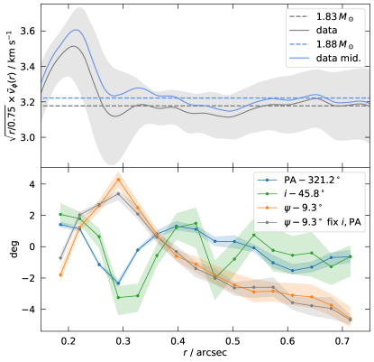
Figure 2: Top: Rotation curve of HD 100546 for the global orientation $i_{\circ}$, PA_∘, $\psi_{\circ}$. The thin grey line traces $\tilde{v}_{\phi}(r)$, and the vertical extension of the shaded area corresponds to twice the scatter of $v_{\circ}(\phi)-v^{m}_{\circ}(\phi)$ (this scatter is $\sim 10\times$ the error on $\tilde{v}_{\phi}(r)$). Comparison Keplerian profiles are shown in dashed lines. Bottom: Orientation of HD 100546, with radial variations in the deviations of PA, $i$, and $\psi$ from their value for the whole radial domain. We also plot $\psi(r)$ when fixing $i=i_{\circ}$ and PA=PA_∘.

The rotation curve $\tilde{v}_{\phi}(r)$ for the global orientation $i_{\circ}$, PA_∘, $\psi(r)$, shown in Fig. 2, is readily comparable with Keplerian profiles (ignoring corrections due to hydrostatic support, e.g. Rosenfeld et al., 2013; Teague et al., 2018), with $v_{K}(r)=\sqrt{GM_{\star}/(r\times d)}$ for a distance $d$. We checked that the impact of calculating $\tilde{v}_{\phi}(r)$ with the radial profiles $i(r)$, PA$(r)$, $\psi(r)$ is small (below 1%). If we assume a constant $\tilde{v}_{\phi}(r)$ independent of height over the midplane, the best fit mass from $0\farcs 15$ to $0\farcs 75$ is $M_{\star}=1.83\pm 0.01\,M_{\odot}$, as measured by minimizing

$$\chi^{2}=\sum_{r}\frac{(v_{K}(r)-\tilde{v}_{\phi}(r))^{2}}{\sigma^{2}(\tilde{v}_{\phi})},$$ (11)

and for a distance of 110.02 pc (Gaia Collaboration et al., 2018). The uncertainties in $M_{\star}$ are estimated using the error on the mean $\sigma(\tilde{v}_{\phi})$, which is smaller than the scatter plotted in Fig. 2 by a factor $\sim 1/\sqrt{N_{b}}\sim 1/10$, where $N_{b}$ is the number of independent data points (i.e the number of clean beams along a fixed radius). The standard deviation of $M_{\star}$ when fitting in narrow radial bins is $\sigma(M_{\star})=0.12\,M_{\odot}$, we adopt this uncertainty to account for systematics. Vertical Keplerian shear, in the extreme case of no vertical viscosity or magnetic coupling, and ignoring radial hydrostatic support, yields midplane azimuthal velocities $\tilde{v}_{\phi}(r)(1+h^{2})^{3/4}$. This is the case labeled ‘data mid.’ in Fig. 2, with a slightly higher $M_{\star}=1.88\pm 0.13\,M_{\odot}$. The deviations of $\tilde{v}_{\phi}(r)$ from $v_{K}(r)$ are much larger than in this midplane extrapolation, and are probably due to the radial pressure gradient. The non-Keplerian rotation curve is particularly pronounced inside a radius of $0\farcs 3$, which could reflect a pressure bump under the continuum ring at the edge of the cavity.

3.2 HD 97048 and HD 163296

Channel-map wiggles in ¹²CO have been identified in HD 163296 (Pinte et al., 2018b), but we could not pick-up the concomitant Doppler-flip in the velocity centroid in these and finer angular resolution data (based on the DSHARP large program data in Isella et al., 2018, see also their velocity centroid). In Fig. 3, the scatter within a radius of $0\farcs 5$ centered at the location of the putative protoplanet is $0.07$ km s^-1, and a factor of $\sim$4 smaller when smoothing to $\sim 50$ au scales (corresponding to the section of the planetary wakes, see Fig. 4 in Pinte et al., 2018b). Thus the total amplitude of any Doppler-flip at the predicted planet location is less than $2\times 0.05$ km s^-1 (at 3$\sigma$). The rotation curve reads $\sim$1.8 km s^-1 at the location of the putative protoplanet, so a flip similar to that in HD 100546 would have an amplitude of $\sim$0.8 km s^-1 and may escape detection. We caution that the spectral resolution of the DSHARP data is rather coarse, $\sim$0.3 km s^-1, so the CO line at the putative protoplanet location is sampled with only 3 spectral points. This limits the accuracy of the Gaussian centroid map. We compute a systemic velocity of $5.79\pm 0.02$ km s^-1, and the global orientation is $\psi_{\circ}=-7.1\pm 2.2$ deg, $i_{\circ}=144.9\pm 2.5$ deg, and PA${}_{\circ}=312.3\pm 0.5$ deg, but we note that this system may be warped by $\sim 6$ deg from $1\farcs 5$ to $3\farcs 5$. The rotation curve bears similar radial hydrostatic support modulations as discussed by Teague et al. (2018). For a distance of 101.5 pc (Gaia Collaboration et al., 2018), a Keplerian fit to observed (surface) $\tilde{v}_{\phi}$ gives $M_{\star}=2.61\pm 0.08\,M_{\odot}$, and the midplane extrapolation gives $M_{\star}=2.67\pm 0.10\,M_{\odot}$, where the uncertainty are due to the hydrostatic support modulations.

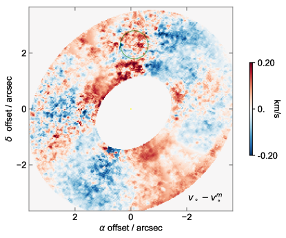
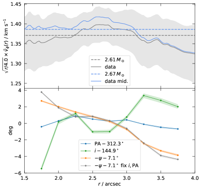
Figure 3: Top: Non-axial velocity field $v_{\circ}-v_{\circ}^{m}$ in HD 163296. Labels follow from Fig. 1d. The green circle is $0\farcs 5$ in radius and is centered on the putative HD 163296b. Bottom: Rotation curve and orientation profile, labels follow from Fig. 2.

We have also performed a similar analysis in HD 97048, using the ¹³CO(3-2) data from program 2016.1.00826.S, (Pinte et al., 2019, in this case the velocity sampling is 0.1 km s^-1). The non-Keplerian flow $v_{\circ}-v_{\circ}^{m}$ is shown in Fig. 4. Any Doppler-flip in this ringed system is drowned by the systematics which result in radial stripes, probably due to our neglect of the far-side. The rotation curve reads $\sim$3 km s^-1 at the location of the putative protoplanet, so a Doppler-flip similar to that in HD 100546 would have an amplitude of $\sim$1.3 km s^-1. The systemic velocity is $v_{s}=4.74\,$km s^-1, and the best fit orientation is $i_{\circ}=39.5\pm 0.75$ deg, PA$=3.4\pm 0.2$ deg, $\psi_{\circ}=11.3\pm 1.3$ deg. For a distance of 184.8 pc (Gaia Collaboration et al., 2018) the Keplerian mass from the midplane extrapolation is $M_{\star}=2.78\pm 0.14\,M_{\odot}$.

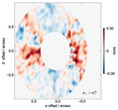
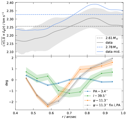
Figure 4: Top: Non-Keplerian flow $v_{\circ}-v_{\circ}^{m}$ in HD 97048. The green circle is centered on the putative HD 97048b. Bottom: Rotation curve and orientation profile. Labels follow from Fig. 3.

4 Conclusion

In an effort to indirectly detect embedded protoplanets using their imprint on planet-disk interactions, we have designed a technique to subtract the axially symmetric flow, or rotation curve, from velocity centroid maps. Our goal was to pick-up protoplanets using the expected Doppler-flip along the spiral wakes. Applications require long-baseline and deep ALMA data. The case of HD 163296, where a protoplanet has previously been proposed based on disk kinematics, yielded a negative result, limited by the measurement accuracy. Any Doppler-flip in ¹²CO at the predicted planet location is less than 0.05 km s^-1 (at 3$\sigma$). Likewise in HD 97048, although these ¹³CO data may require a more refined averaging procedure. However, an application to the ¹²CO data in HD 100546 from paper I yielded a very conspicuous Doppler-flip, whose properties match the expectations for a spiral wake in planet-disk interactions in extension and in velocity sign, but not in pitch-angle. Its coincidence with a fine ridge crossing a shallow groove inside the continuum ring suggest a complex dynamical scenario, and should inspire dedicated 3D gas+dust hydrodynamic simulations.

References

- Boccaletti et al. (2013) Boccaletti, A., Pantin, E., Lagrange, A.-M., Augereau, J.-C., Meheut, H., & Quanz, S. P. 2013, A&A, 560, A20
- Brittain et al. (2014) Brittain, S. D., Carr, J. S., Najita, J. R., Quanz, S. P., & Meyer, M. R. 2014, ApJ, 791, 136
- Cárcamo et al. (2018) Cárcamo, M., Román, P. E., Casassus, S., Moral, V., & Rannou, F. R. 2018, Astronomy and Computing, 22, 16
- Czekala et al. (2015) Czekala, I., Andrews, S. M., Jensen, E. L. N., Stassun, K. G., Torres, G., & Wilner, D. J. 2015, ApJ, 806, 154
- Czekala et al. (2016) Czekala, I., Andrews, S. M., Torres, G., Jensen, E. L. N., Stassun, K. G., Wilner, D. J., & Latham, D. W. 2016, ApJ, 818, 156
- Dong & Fung (2017) Dong, R., & Fung, J. 2017, ApJ, 835, 146
- Dong et al. (2018) Dong, R., Li, S., Chiang, E., & Li, H. 2018, ApJ, 866, 110
- Dong et al. (2019) Dong, R., Liu, S.-Y., & Fung, J. 2019, ApJ, 870, 72
- Dullemond et al. (2015) Dullemond, C., Juhasz, A., Pohl, A., Sereshti, F., Shetty, R., Peters, T., Commercon, B., & Flock, M. 2015, RADMC3D v0.41 http://www.ita.uni-heidelberg.de/ dullemond/software/radmc-3d/
- Foreman-Mackey et al. (2013) Foreman-Mackey, D., Hogg, D. W., Lang, D., & Goodman, J. 2013, PASP, 125, 306
- Gaia Collaboration et al. (2018) Gaia Collaboration et al. 2018, A&A, 616, A1
- Garufi et al. (2016) Garufi, A., et al. 2016, A&A, 588, A8
- Goldreich & Tremaine (1980) Goldreich, P., & Tremaine, S. 1980, ApJ, 241, 425
- Huang et al. (2018) Huang, P., Isella, A., Li, H., Li, S., & Ji, J. 2018, ApJ, 867, 3
- Isella et al. (2018) Isella, A., et al. 2018, ApJ, 869, L49
- Keppler et al. (2018) Keppler, M., et al. 2018, A&A, 617, A44
- Lin & Papaloizou (1980) Lin, D. N. C., & Papaloizou, J. 1980, MNRAS, 191, 37
- Liu et al. (2019) Liu, B., Ormel, C. W., & Johansen, A. 2019, A&A, 624, A114
- Morbidelli et al. (2014) Morbidelli, A., Szulágyi, J., Crida, A., Lega, E., Bitsch, B., Tanigawa, T., & Kanagawa, K. 2014, Icarus, 232, 266
- Pérez et al. (2018) Pérez, S., Casassus, S., & Benítez-Llambay, P. 2018, MNRAS, 480, L12
- Perez et al. (2015) Perez, S., Dunhill, A., Casassus, S., Roman, P., Szulágyi, J., Flores, C., Marino, S., & Montesinos, M. 2015, ApJ, 811, L5
- Pinte et al. (2018a) Pinte, C., et al. 2018a, A&A, 609, A47
- Pinte et al. (2018b) —. 2018b, ApJ, 860, L13
- Pinte et al. (2019) —. 2019, arXiv e-prints, arXiv:1907.02538
- Rosenfeld et al. (2013) Rosenfeld, K. A., Andrews, S. M., Hughes, A. M., Wilner, D. J., & Qi, C. 2013, ApJ, 774, 16
- Rosenfeld et al. (2012) Rosenfeld, K. A., Andrews, S. M., Wilner, D. J., & Stempels, H. C. 2012, ApJ, 759, 119
- Teague et al. (2018) Teague, R., Bae, J., Bergin, E. A., Birnstiel, T., & Foreman-Mackey, D. 2018, ApJ, 860, L12
- Zhu & Baruteau (2016) Zhu, Z., & Baruteau, C. 2016, MNRAS, 458, 3918
- Zhu et al. (2015) Zhu, Z., Dong, R., Stone, J. M., & Rafikov, R. R. 2015, ApJ, 813, 88