On the discontinuity of the quantum Fisher information for quantum statistical models with parameter dependent rank

Abstract

We address the discontinuities of the quantum Fisher information (QFI) that may arise when the parameter of interest takes values that change the rank of the quantum statistical model. We revisit the classical and the quantum Cramér-Rao theorems, show that they do not hold in these limiting cases, and discuss how this impacts on the relationship between the QFI and the Bures metric. In order to illustrate the metrological implications of our findings, we present two paradigmatic examples, where we discuss in detail the role of the discontinuities and show that the Cramér-Rao may be easily violated.

1 Introduction

A quantum metrological protocol is a detection scheme where the inherent fragility of quantum systems to external perturbations is exploited to enhance precision, stability or resolution in the estimation of one or more quantities of interest. In the last two decades, the development of advanced technologies to coherently manipulate quantum systems, and to address them with unprecedented accuracy, made it possible to realize several metrological schemes based on quantum systems, leading to quantum enhanced high-precision measurements of physical parameters [1].

On the theoretical side, the main tool of quantum metrology is the so-called quantum Cramér-Rao theorem, stating that for a regular quantum statistical model the precision is bounded by the inverse of the quantum Fisher information (QFI) [2, 3, 4, 5, 6, 7]. Evaluating the QFI thus provides the ultimate quantum limits to precision, and a general benchmark to assess metrological protocols. The quantum Cramér-Rao theorem is indeed a very powerful tool, and it has found a widespread use in quantum metrology. At the same time, its success has lead to somehow overlooking the mathematical details of its hypotheses, such as a possible intrinsic parameter dependence of the measurement apparatus [8, 9] or the pathological situations that may occur when the parameter of interest takes values that change the rank of density matrix of the system. In such quantum statistical models, analogous to non-regular models in classical statistics, the QFI may show discontinuities, which undermine the validity of the Cramér Rao theorem and, in turn, its use in quantum metrology.

In this paper, we consider statistical models whose rank is a non-trivial function of the parameter to be estimated. We address the discontinuities of classical and quantum Fisher information and revisit both the classical and the quantum Cramér-Rao theorems, showing that they do not hold in these limiting cases, also discussing how this reflects on the relationship between the QFI and the Bures metric. In order to illustrate the metrological implications of our findings, we also discuss two paradigmatic examples, where the Cramér-Rao bound may be easily violated.

Let $\rho_{\theta}$ denote a quantum statistical model with parameter space $\Theta$. Suppose that $\bar{\theta}$ is the true value of the parameter and that, in any open neighbourhood $N_{\bar{\theta}}$ of $\bar{\theta}$, there exists $\theta^{\prime}$ such that $\text{rank}(\rho_{\theta^{\prime}})\neq\text{rank}(\rho_{\bar{\theta}})$. The typical situation is when the rank changes at an isolated point $\bar{\theta}$ of $\Theta$, but more general situations may also be envisioned. This apparently harmless circumstance causes new theoretical challenges in determining the best performance of any quantum estimation strategy. Nonetheless, it is a situation of physical interest that might naturally arise when estimating noise parameters, e.g. in the estimation of momentum diffusion induced by collapse models under continuous monitoring of the environment [10]. We will show that this scenario also applies to an instance of frequency estimation with open quantum systems [11].

The consequences of allowing the rank to vary with $\theta$ can be severe, both from a geometrical and a statistical perspective. From the geometrical point of view, it is known that the Fisher information metric may develop discontinuities [12] and suitable regularization techniques have been proposed for specific classes of states [13, 14]. On the other hand, the question of how such discontinuities affect the statistical estimation problem at hand is currently open [12]. In the following, we are going to argue that the standard theory based on the Cramér-Rao bound breaks down at such points of the parameter space where the rank of $\rho_{\theta}$ changes. In fact, such a failure of the standard theory is not specific to quantum statistical models, but is actually present already at the classical level [15, 16, 17]

1.1 Classical and quantum regular models

In order to establish notation, let us briefly review the regular scenario, which is the theoretical foundation to most applications in classical and quantum metrology. We assume that the quantum parametrization maps $\varphi_{\theta}:\,\theta\to\rho_{\theta}$ or the classical one $\varphi_{\theta}:\,\theta\to p_{\theta}$ are sufficiently well-behaved, such that the symmetric logarithmic derivative $L_{\theta}$, implicitly defined via the relation $\partial_{\theta}\rho_{\theta}=\{\rho_{\theta},\,L_{\theta}\}/2$ or the classical score function $\ell_{\theta}=\partial_{\theta}\log p_{\theta}$ exist and the corresponding quantum and classical Fisher information metrics are well-defined and finite, $\forall\theta\in\Theta$.

Setting apart all pathological situations where these conditions do not hold, e.g. the statistical model is non-differentiable or even discontinuous (see [18, 19] for such a scenario in quantum estimation), we further qualify a quantum statistical model as regular if it satisfies the following conditions: 1. fixed-rank: the rank of the statistical model $\rho_{\theta}$ (i.e. the rank of the density matrices $\rho_{\theta}$) is independent of $\theta$; 2. identifiable: the parametrization map $\varphi_{\theta}:\,\theta\to\rho_{\theta}$ is injective; 3. non-singular metric: the Fisher-Bures metric $g_{\theta}$, defined by $2[1-F(\rho_{\theta},\rho_{\theta+\epsilon})]=g_{\theta}\,\epsilon^{2}+O(\epsilon^{3})$, where $F(\rho,\sigma)=\tr\left[\sqrt{\sqrt{\rho}\sigma\sqrt{\rho}}\right]$ is the quantum fidelity, is a well-defined positive-definite function $\forall\theta\in\Theta$.

Let us also give the translation of the previous definition to the classical setting. A regular classical statistical model $p_{\theta}$ satisfies the following conditions: 1. parameter-independent support: the support $\text{supp}(p_{\theta})$ of the statistical model (i.e. the subset of the real axis where $p_{\theta}\neq 0$) is independent of $\theta$; 2. identifiable: the coordinate map $\varphi_{\theta}:\,\theta\to p_{\theta}$ is injective; 3. non-singular metric: the Fisher-Rao information metric $f_{\theta}$, defined by $2D(p_{\theta}||p_{\theta+\epsilon})=f_{\theta}\,\epsilon^{2}+O(\epsilon^{3})$, where $D(p||q)=\sum_{x}p_{x}\log p_{x}/q_{x}$ is the Kullback-Leibler divergence, is a well-defined positive-definite function $\forall\theta\in\Theta$.

For regular statistical models, one has the following results, which provide the standard tools of current classical and quantum metrology

Proposition 1.

Given a regular classical statistical model $p_{\theta}$,

• For any unbiased estimator $\hat{\theta}$, the Cramér-Rao bound $\text{Var}_{\theta}(\hat{\theta})\geq\left(M\,\mathcal{F}_{\theta}\right)^{-1}$ holds, where $M$ is the number of repetitions and $\mathcal{F}_{\theta}$ the Fisher information,

  $$\mathcal{F}_{\theta}=\sum_{y}\frac{\left[\partial_{\theta}p_{\theta}(y)\right]^{2}}{p_{\theta}(y)}$$ (1)

• The Cramér-Rao bound is attainable: i) for finite $M$, if $p_{\theta}$ belongs to the exponential family and $\theta$ is a natural parameter of $p_{\theta}$, by the unique efficient estimator of $\theta$ ii) asymptotically, as $M\to\infty$, e.g. by the maximum-likelihood or Bayes estimators.

• The maximum-likelihood and Bayes estimators have the asymptotic normality property, i.e. $\sqrt{M}(\hat{\theta}-\theta)\overset{d}{\to}\,N(0,1/\mathcal{F}_{\theta})$ as $M\to\infty$.

In addition, we have that $\mathcal{F}_{\theta}=f_{\theta}$ i.e the Fisher information equals the Fisher-Rao metric.

Proposition 2.

Given a regular quantum statistical model $\rho_{\theta}$,

• For any quantum measurement $\{\Pi_{x}\}_{x\in\mathcal{X}}$, $\sum_{x\in\mathcal{X}}\Pi_{x}=\mathbbm{I}$ and unbiased estimator $\hat{\theta}$, the quantum Cramér-Rao bound $\text{Var}_{\theta}(\hat{\theta})\geq\left(M\,\mathcal{Q}_{\theta}\right)^{-1}$ holds, where $M$ is the number of repetitions, $\mathcal{Q}_{\theta}$ the quantum Fisher information,

  $$\mathcal{Q}_{\theta}=\tr[\rho_{\theta}L_{\theta}^{2}]\,$$ (2)

  and $L_{\theta}$ is the symmetric logarithmic derivative (SLD) operator, defined via the Lyapunov equation $2\partial_{\theta}\rho_{\theta}=L_{\theta}\rho_{\theta}+\rho_{\theta}L_{\theta}$.

• The quantum Cramér-Rao bound is attainable by implementing the optimal Braunstein-Caves measurement, i.e. a projective measurement of the symmetric logarithmic derivative $L_{\theta}$, and under the conditions stated before for the resulting classical statistical model.

By considering the spectral decomposition of the quantum statistical model $\rho_{\theta}=\sum_{k}\lambda_{k,\theta}|\lambda_{k,\theta}\rangle\langle\lambda_{k,\theta}|$, one obtains that the SLD operator can be written as [7]

$$L_{\theta}=2\sum_{\tiny{\lambda_{k,\theta}+\lambda_{l,\theta}>0}}\frac{\langle\lambda_{k,\theta}|\partial_{\theta}\rho_{\theta}|\lambda_{l,\theta}\rangle}{\lambda_{k,\theta}+\lambda_{l,\theta}}|\lambda_{k,\theta}\rangle\langle\lambda_{l,\theta}|\,,$$ (3)

and consequently the QFI can be evaluated as

$$\mathcal{Q}_{\theta}=2\sum_{\tiny{\lambda_{k,\theta}+\lambda_{l,\theta}>0}}\frac{|\langle\lambda_{k,\theta}|\partial_{\theta}\rho_{\theta}|\lambda_{l,\theta}\rangle|^{2}}{\lambda_{k,\theta}+\lambda_{l,\theta}}\,.$$ (4)

Moreover, the QFI is proportional to the Fisher-Bures metric

$$\mathcal{Q}_{\theta}=4g_{\theta}\,.$$ (5)

We remark that for non full-rank quantum models the Lyapunov equation does not have a unique solution. Nonetheless, there is no ambiguity in the definition of the QFI for fixed-rank models, since the unspecified components of the SLD do not play any role in Eq. (2) [3, 20].

2 Non-regular case

If either of the three regularity conditions listed above is not true, Props. 1 and 2 do not hold. The second condition, if not verified, can often be realized by simply restricting the parameter space $\Theta$ or by a change of parametrization. Let us consider a trivial example, i.e. the statistical model $\rho_{\theta}=\sin^{2}\theta\ket{0}\bra{0}+\cos^{2}\theta\ket{1}\bra{1}$. If we consider $\theta\in\mathbbm{R}$, the model is not identifiable, but it can be made so by restricting the values of $\theta$ to the interval $[0,\pi/2]$. In a non-identifiable model, the true value of the parameter is in general non-unique, therefore a local approach becomes impossible and the Cramér-Rao bound is meaningless.

Let us now assume that the model is identifiable, or can be made so by a suitable reparametrization. However, the rank of the statistical model, or its support in the classical case, is allowed to vary by varying the parameter $\theta$.

2.1 Variable-rank models

Let us start from the classical case, since our conclusions may then be translated to the quantum case. Denote by $\mathcal{X}_{\theta}$ the support of $p_{\theta}$, i.e. the closure of the set $\{x\,|\,p_{\theta}(x)>0\}$. Let’s see why the derivation of the Cramér-Rao bound breaks down. For simplicity, fix $M=1$. Given any two statistics $t_{1}$ and $t_{2}$, their inner product is defined in terms of the probability distribution $p_{\theta}(x)$ as

$$\langle t_{1},\,t_{2}\rangle=\mathbbm{E}_{\theta}(t_{1}t_{2})=\int_{\mathcal{X}_{\theta}}dx\,p_{\theta}(x)t_{1}(x)t_{2}(x)\;.$$ (6)

Take $t_{1}(x)=\hat{\theta}(x)-\theta$ and $t_{2}(x)=\partial_{\theta}\log p_{\theta}(x)$. Then, by the Cauchy-Schwarz inequality $\langle t_{1},\,t_{2}\rangle^{2}\leq\langle t_{1},\,t_{1}\rangle\langle t_{2},\,t_{2}\rangle$, one obtains

$$\int_{\mathcal{X}_{\theta}}dx\,[\hat{\theta}(x)-\theta]\,\partial_{\theta}p_{\theta}(x)\leq\text{Var}_{\theta}(\hat{\theta})\cdot\mathcal{F}_{\theta}\;.$$ (7)

Now, if $\mathcal{X}_{\theta}$ were independent of $\theta$, and under very mild assumptions regarding the smoothness of $p_{\theta}$, one could interchange the order of integration and differentiation, and conclude that the LHS is equal to 1, which would imply the Cramér-Rao bound. However, the very fact that $\mathcal{X}_{\theta}$ depends on $\theta$ prevents one from performing the optimization over all possible estimators $\hat{\theta}$ of the parameter The conclusion is that the Fisher information is not directly linked to the best possible performance over the set of unbiased estimators.

Moving to the quantum case, since the quantum Fisher information is the Fisher information corresponding to the optimal measurement [5, 4], it is also not directly linked to the best possible performance over the set of quantum estimation strategies. Notice that both the Fisher information and the quantum Fisher information are still well-defined even at the point $\bar{\theta}$ where the rank changes. They could, however, develop a discontinuity there.

2.2 Discontinuity of classical and quantum Fisher information

Suppose now that the statistical model $p_{\theta}$ describes the p.m.f. of a discrete random variable $X$ and that, as $\theta\to\bar{\theta}$, the probability $p_{\theta}(\bar{y})$ of one of its outcomes $\bar{y}\in\mathcal{X}$ goes to zero. Since the Fisher information is computed only on the support of the model, it follows that

$$\Delta\mathcal{F}=\lim_{\theta\to\bar{\theta}}\mathcal{F}_{\theta}-\mathcal{F}_{\bar{\theta}}=\lim_{\theta\to\bar{\theta}}\frac{[\partial_{\theta}p_{\theta}(\bar{y})]^{2}}{p_{\theta}(\bar{y})}.$$ (8)

If the limit on the RHS is non-zero, then the Fisher information is discontinuous.

Proposition 3.

The Fisher information $\mathcal{F}_{\theta}$ at $\theta=\bar{\theta}$ is continuous if both the speed $v=\lim_{\theta\to\bar{\theta}}\partial_{\theta}p_{\theta}(y)$ and the acceleration $a=\lim_{\theta\to\bar{\theta}}\partial_{\theta}^{2}p_{\theta}(y)$ with which $p_{\theta}(y)\to 0$ are zero. Otherwise, if $v=0$ but $a\neq 0$, the discontinuity is equal to $\Delta\mathcal{F}=2a$ and if $v\neq 0$ there is a discontinuity of the second kind.

Proof.

Follows from L’Hôpital’s rule. ∎

We now move to the quantum case and suppose that the rank of the quantum statistical model $\rho_{\theta}$ diminishes by one at $\theta=\bar{\theta}$ because one of its eigenvalues $\lambda_{m,\theta}$ vanishes as $\theta\to\bar{\theta}$. Is the quantum Fisher information discontinuous as $\theta\to\bar{\theta}$? By looking at the formula in Eq. (4), one sees that the discontinuity can be evaluated as (in the following we are omitting the dependence on $\theta$ of eigenvalues and eigenvectors)

$$\Delta\mathcal{Q} =\lim_{\theta\to\bar{\theta}}\mathcal{Q}_{\theta}-\mathcal{Q}_{\bar{\theta}}$$ (9)

$$=\lim_{\theta\to\bar{\theta}}\left(4\sum_{\tiny{\lambda_{k}=0}}\frac{|\langle\lambda_{k}|\partial_{\theta}\rho_{\theta}|\lambda_{m}\rangle|^{2}}{\lambda_{m}}+2\,\frac{|\langle\lambda_{m}|\partial_{\theta}\rho_{\theta}|\lambda_{m}\rangle|^{2}}{2\lambda_{m}}\,.\right)$$ (10)

By analyzing the first term, where the sum runs over the kernel of the statistical model $\rho_{\theta}$, we observe

$$\frac{|\langle\lambda_{k}|\partial_{\theta}\rho_{\theta}|\lambda_{m}\rangle|^{2}}{\lambda_{m}} =\frac{1}{\lambda_{m}}|\langle\lambda_{k}|\partial_{\theta}\lambda_{m}\rangle|^{2}\,|\langle\lambda_{m}|\lambda_{m}\rangle|^{2}\,\lambda_{m}^{2}$$

$$=\lambda_{m}|\langle\lambda_{k}|\partial_{\theta}\lambda_{m}\rangle|^{2}\underset{\theta\to\bar{\theta}}{\to}0\,,$$ (11)

as, by hypothesis, $\displaystyle\lim_{\theta\to\bar{\theta}}\lambda_{m}=0$. The second term, by exploiting the orthogonality of the eigenstates of $\rho_{\theta}$, reads

$$\frac{|\langle\lambda_{m}|\partial_{\theta}\rho_{\theta}|\lambda_{m}\rangle|^{2}}{\lambda_{m}} =\frac{|\langle\lambda_{m}|\partial_{\theta}(\lambda_{m}|\lambda_{m}\rangle\langle\lambda_{m}|)|\lambda_{m}\rangle|^{2}}{\lambda_{m}}$$

$$=\frac{(\partial_{\theta}\lambda_{m})^{2}}{\lambda_{m}}+2\lambda_{m}|\langle\partial_{\theta}\lambda_{m}|\lambda_{m}\rangle|^{2}\underset{\theta\to\bar{\theta}}{\to}\frac{(\partial_{\theta}\lambda_{m})^{2}}{\lambda_{m}}\,.$$ (12)

We are thus left with the following proposition:

Proposition 4.

The quantum Fisher information $\mathcal{Q}_{\theta}$ at $\theta=\bar{\theta}$ is continuous if both the speed $v=\lim_{\theta\to\bar{\theta}}\partial_{\theta}\lambda_{m}$ and the acceleration $a=\lim_{\theta\to\bar{\theta}}\partial_{\theta}^{2}\lambda_{m}$ with which the eigenvalue $\lambda_{m}$ is vanishing are zero. Otherwise, if $v=0$ but $a\neq 0$, the discontinuity is equal to $\Delta\mathcal{Q}=2a$ and if $v\neq 0$ there is a discontinuity of the second kind.

The discontinuity of the QFI in variable-rank models have been addressed in [12], where in particular it was shown that the continuous version of the standard QFI is proportional to the Bures metric, i.e.

$$\lim_{\theta\to\bar{\theta}}\mathcal{Q}_{\theta}=4g_{\theta}\,.$$ (13)

This means that the Fisher-Bures metric can be exploited to evaluate the QFI only for regular models whereas for non regular ones this link is broken. In addition, as we pointed out above, the hypotheses at the basis of the derivation of the classical and quantum Cramér-Rao bounds do not hold for this kind of models, and consequently these bounds can be violated and are of no use in quantum metrology. To better describe this issue, in the next section we provide two quantum estimation problems falling into these models. In both cases, we will show that the QFI is in fact discontinuous and, in turn, it is easy to construct an estimator with zero variance in the case $\theta=\bar{\theta}$.

3 Examples of quantum statistical models with parameter dependent rank

Let us now illustrate two paradigmatic examples of variable-rank quantum statistical models: a model that can be mapped to a classical statistical model, such as the ones discussed in [12], and a genuinely quantum statistical model.

3.1 A classical quantum statistical model

A quantum statistical model is said classical, if the family of quantum states $\rho_{\theta}$ can be diagonalized with a $\theta$-independent unitary, and thus the whole information on the parameter is contained in the eigenvalues [21].
The simplest example of classical model is described by the family of two-dimensional quantum states

$$\rho_{p}=p|0\rangle\langle 0|+(1-p)|1\rangle\langle 1|\,,\,\,\,\,\,0\leq p\leq 1\,.$$ (14)

As it is apparent, this is also a variable-rank statistical model, when the parameter to be estimated $p$ takes the limiting values $\bar{p}=\{0,1\}$. For a generic value of the parameter between the two limiting values, $0<p<1$, the QFI reads

$$\mathcal{Q}_{p}=\frac{1}{p(1-p)}\,,$$ (15)

while in the two limiting values $\bar{p}$, one gets $\mathcal{Q}_{\bar{p}}=1$. As expected, one observes a discontinuity of the second kind, and in particular an infinite Bures metric, $\lim_{p\rightarrow\bar{p}}g_{p}=\infty$.

The optimal measurement corresponds trivially to the projections on the states $\{|0\rangle\langle 0|,|1\rangle\langle 1|\}$ and clearly does not depend on the parameter to be estimated. For the limiting values, it is easy to check that a maximum likelihood estimator would give a variance equal to zero (in fact one always gets the same measurement outcome). It is well known that the estimation of parameters on the boundary of the parameter space breaks down the asymptotic normality of the maximum-likelihood estimator as well as the validity of the Cramér-Rao bound [22, 23, 24, 25, 26].

Therefore, while on the one hand it should be now clear that no Cramér-Rao bound holds in these instances, on the other hand this result would induce to say that the Bures metric gives the correct figure of merit to asses the performances for $\theta\to\bar{\theta}$. However, this is not always the case: one could check that by reparametrizing the family of states to [12]

$$\rho_{\theta}=\sin^{2}\theta|0\rangle\langle 0|+\cos^{2}\theta|1\rangle\langle 1|\,,$$ (16)

one would obtain that the Bures metric is identically equal for all values of $\theta$, $g_{\theta}=1$, while the standard QFI is discontinuous and reads

$$\mathcal{Q}_{\theta}=\left\{\begin{array}[]{c}4\,\,\,\,\theta\neq k\pi/2\\ 0\,\,\,\,\theta=k\pi/2\\ \end{array}\right.$$ (19)

However, also in this case the optimal measurement and the maximum likelihood estimator would trivially give a zero variance estimation (at least if we restrict the values of $\theta$ to $[0,\pi/2]$, so that the model becomes identifiable). In turn, the Cramér-Rao bound is violated.

We mention that from an heuristic point of view, one may conjecture that in these classical cases, it is always possible to find a parametrization such that the corresponding Bures metric is infinite, thus suggesting that a zero variance estimation may be approached continuously for parameter values near the critical one.

3.2 A genuine quantum statistical model

Let us now consider the quantum statistical model described by a family of two-dimensional quantum states $\rho_{\theta}$ that solve the Markovian master equation

$$\frac{d\rho_{\theta}}{dt}=-i\frac{\theta}{2}[\sigma_{z},\rho_{\theta}]+\frac{\kappa}{2}(\sigma_{x}\rho\sigma_{x}-\rho)\,,$$ (20)

with initial condition $\rho_{\theta}(t=0)=|+\rangle\langle+|$, where $|+\rangle=(|0\rangle+|1\rangle)/\sqrt{2}$ denotes the eigenstate of the x-Pauli matrix $\sigma_{x}$ in terms of the eigenstates of the z-Pauli matrix $\sigma_{z}$. From a physical point of view this master equation describes the evolution of a spin-$1/2$ system, subjected to a phase-rotation due to a magnetic field proportional to $\theta$ along the $z$-direction and subjected to transverse noise along the $x$-direction with rate $\kappa$.

The master equation can be solved analytically and the corresponding QFIs, $\mathcal{Q}_{\theta}$ and $\mathcal{Q}_{\theta}^{(B)}$, can be readily evaluated. For the parameter value $\bar{\theta}=0$, one observes how the master equation has no effect on the initial state $|+\rangle$ (the Pauli matrix $\sigma_{x}$ clearly commutes with its eigenstate $|+\rangle\langle+|$). As a consequence, for $\bar{\theta}=0$, the quantum state remains pure (and identical to the initial state) during the whole evolution, showing how the rank of the corresponding quantum statistical model changes by considering a non-zero frequency $\theta\neq 0$. Remarkably, unlike the previous example, both eigenstates and eigenvalues of $\rho_{\theta}$ depend on the parameter $\theta$; in this sense, the quantum statistical model cannot be readily mapped in a classical one.

The QFIs at the discontinuity point $\theta=\bar{\theta}$ can be analytically evaluated as

$$\mathcal{Q}_{\bar{\theta}=0} =4\frac{e^{-\kappa t}\sinh^{2}\frac{\kappa t}{2}}{\kappa^{2}}\,$$ (21)

$$g_{\bar{\theta}=0} =2\frac{e^{-\kappa t}+\kappa t-1}{\kappa^{2}}\,.$$ (22)

One can check that the eigenvalue of $\rho_{\theta}$ that goes to zero for $\theta\rightarrow 0$ is equal to

$$\lambda=\frac{1}{2}\left(1+\frac{e^{-\frac{\kappa t}{2}}\sqrt{\kappa^{2}\cosh(\xi t)+\kappa\xi\sinh(\xi t)-4\theta^{2}}}{\xi}\right)\,,$$ (23)

where $\xi=\sqrt{\kappa^{2}-4\theta^{2}}$. The corresponding speed and acceleration reads

$$v =\lim_{\theta\rightarrow 0}\partial_{\theta}\lambda=0\,,$$ (24)

$$a =\lim_{\theta\rightarrow 0}\partial_{\theta}^{2}\lambda=\frac{2\kappa t+4e^{-\kappa t}-e^{-2\kappa t}+3}{\kappa^{2}}\,.$$ (25)

It is then easy to check that, as predicted by Proposition 4, one gets $\Delta\mathcal{Q}=2a$.

If one performs the optimal measurement for $\theta=0$, that trivially corresponds to the projection on eigenstates of the Pauli operator $\sigma_{x}$, one can build a maximum likelihood estimator yielding a zero variance. However it is important to remark that, contrarily to the previous example, in this model, the optimal measurement generally depends on the true value of the parameter $\theta$, and it has to be implemented via an adaptive strategy. This adaptive scheme will approximate the optimal measurement only asymptotically, while for arbitrarily large but finite number of measurements $M$, one will implement a strategy $\epsilon$-close to the optimal one [6, 27, 28]. We thus expect that the corresponding variance of the optimal estimator will be bounded by (four times) the continuous Bures metric $g_{\bar{\theta}}$ obtained via the limit of $\theta$ going to $\bar{\theta}$, and that one should consider this figure of merit to quantify the overall performance of the estimation process.

It is worth to remark that this quantum statistical model can be generalized to $N$ qubits. In Appendix A, for an initial GHZ state, we evaluate the limit of the QFI for $\theta\to 0$, i.e. the Bures metric in $\theta=0$, as well as the discontinuous QFI obtained for $\theta=0$ and we underline a markedly different behavior of the two quantities as functions the probing time $t$. Incidentally, the limit of the QFI for $\theta\to 0$ is exactly the ultimate QFI, obtained by optimizing over all the possible measurements on the system and the environment causing the non-unitary dynamics [29, 30, 31]. In such a framework, this quantity represents a valid statistical bound for all values of $\theta$.

4 Conclusion

The quantum Cramér-Rao theorem is regarded as the foundation of quantum estimation theory, promoting the QFI and the Bures metric as the two fundamental figures of merit that one should consider in order to obtain the ultimate precision achievable in the estimation of parameters in quantum systems. In this manuscript we have addressed variable-rank quantum statistical models and the corresponding discontinuity of the QFI. While this topic has been addressed before in the literature [12], the validity of the quantum Cramér-Rao theorem was not properly discussed. Here, we have shown in detail that the proof of the theorem in fact breaks down in these pathological cases both in the classical and quantum case; as a consequence, the bound can be no longer considered valid. We have also addressed two paradigmatic examples, and considered the corresponding behaviour of the QFI, of the Bures metric and of the variance of the maximum likelihood estimator. While in regular cases these quantities typically coincide, we have shown how they may differ in the presence of a discontinuity and identified the most relevant quantities to consider for these examples. Our results, apart from contributing to clarifying previous results on the discontinuity of the QFI, pave the way to further studies on the relationships between optimal estimators and Bures metric in non-regular quantum statistical models.

Appendix A Discontinuity for frequency estimation with N-qubit GHZ states in transverse independent noise

The calculation presented in this Appendix is hinted, but not included, in Ref. [30]; we also mention that frequency estimation with transverse noise and a vanishing parameter was also considered in Appendix D of [32], but without highlighting the appearance of a discontinuity.

A.1 Evolution of a GHZ state in transverse noise

Greenberg-Horne-Zeilinger (GHZ) states are the prototypical example of states showing a quantum advantage in metrology. Furthermore, they have a particularly simple evolution under independent noises acting on the qubits [33, 34]. In particular, we consider a $N$-qubit GHZ state

$$|\psi_{\mathsf{GHZ}}\rangle=(|0\rangle^{\otimes N}+|1\rangle^{\otimes N})/\sqrt{2}\;,$$ (26)

evolving according to a $N$-qubit version of the master equation (20):

$$\frac{d\rho}{dt}=-i\frac{\theta}{2}\sum_{j}^{N}\left[\sigma_{z}^{(j)},\rho\right]+\frac{\kappa}{2}\left(\sum_{j=1}^{N}\sigma_{x}^{(j)}\rho\sigma_{x}^{(j)}-N\rho\right)\;,$$ (27)

where the the superscript $(j)$ labels operators acting on the $j$-th qubit (i.e. tensored with the identity on all the other qubits). The evolved state $\rho$ becomes a mixture of states of the form $|s\rangle\pm|\bar{s}\rangle$, where $s$ is a binary string and $\bar{s}$ is its bitwise negation, e.g $\ket{s}=\ket{00101}$ and $\ket{\bar{s}}=\ket{11010}$. In the computational basis the density matrix maintains a cross-diagonal form.

It is clever to parametrise the matrix elements with an index $m\in[0,N]$, which counts how many $1$s appear in the binary string $s$, i.e. the sum of the binary representation of $s$. Since we have $N$ qubits there are $2^{N}$ different possible strings, and there are $\binom{N}{m}$ different binary strings that sum to the value $m$, so that $\sum_{m=0}^{N}\binom{N}{m}=2^{N}$. It turns out that the matrix elements of an evolved GHZ state only depend the value $m$. With such a parametrization we have the following matrix elements [35]

$$\begin{split}\rho_{m,m}&=\frac{1}{2}\left[d^{m}a^{N-m}+d^{N-m}a^{m}\right]\\ \rho_{m,N-m}&=\frac{1}{2}\left[f^{m}\left(b-ic\right)^{N-m}+f^{N-m}\left(b+ic\right)^{m}\right],\end{split}$$ (28)

where we can further notice the symmetry of the diagonal terms under the exchange $m\to N-m$. The coefficients appearing in the expression are given by

$$a=\frac{1}{2}\left(1+e^{-\kappa t}\right)\qquad d=\frac{1}{2}\left(1-e^{-\kappa t}\right)\qquad b=e^{-\frac{\kappa t}{2}}\cosh\left(\frac{t}{2}\sqrt{\kappa^{2}-4\theta^{2}}\right)$$ (29)

$$f=\kappa\frac{e^{-\frac{\kappa t}{2}}\sinh\left(\frac{t}{2}\sqrt{\kappa^{2}-4\theta^{2}}\right)}{\sqrt{\kappa^{2}-4\theta^{2}}}\qquad c=2\theta\frac{e^{-\frac{\kappa t}{2}}\sinh\left(\frac{t}{2}\sqrt{\kappa^{2}-4\theta^{2}}\right)}{\sqrt{\kappa^{2}-4\theta^{2}}}.$$

All these coefficients are real as long as $\theta<\frac{\kappa}{2}$, which is the case we are interested in, since we want to take the limit $\theta\to 0$.

A.1.1 Piecewise QFI for a qubit

The QFI for qubit states can be very conveniently written via the Bloch representation of qubit states [36]:

$$\rho=\frac{1}{2}\left(\mathbbm{1}+\vec{v}\cdot\vec{\sigma}\right);$$ (30)

the QFI is easily expressed in terms of the Bloch vector $\vec{v}$

$$\mathcal{Q}_{\theta}\left[\rho\right]=\begin{cases}\left|\partial_{\theta}\vec{v}\right|^{2}+\frac{|\partial_{\theta}\vec{v}\cdot\vec{v}|^{2}}{1-|\vec{v}|^{2}}\qquad&|\vec{v}|<1\\ \left|\partial_{\theta}\vec{v}\right|^{2}&|\vec{v}|=1.\end{cases}$$ (31)

From this piecewise definition it is easy to see the possibility of a discontinuity. In particular, for a qubit the only possible change of rank is that for $\bar{\theta}$ the state becomes pure, i.e. $|\vec{v}|=1$ and so the $\lim_{\theta\to\bar{\theta}}$ gives rise to a $\frac{0}{0}$ indeterminate form; we can then use L’Hôpital’s rule and get

$$\lim_{\theta\to\bar{\theta}}\mathcal{Q}_{\theta}\left[\rho\right]=-\vec{v}\cdot\partial^{2}_{\theta}\vec{v}|_{\theta=\bar{\theta}}.$$ (32)

A.2 Continuous and discontinuous QFI

Given the cross structure of the evolved density matrix and the symmetry of the elements (28), we can reshuffle the $2^{N}\times 2^{N}$ density matrix and write it as the direct sum of $2\times 2$ matrices defined as follows

$$\varsigma_{m}=\begin{pmatrix}\rho_{m,m}&\rho_{m,N-m}\\ \rho_{m,N-m}^{*}&\rho_{m,m}\\ \end{pmatrix},$$ (33)

where now we need only half the values of the index $m=0,\dots,\lfloor N/2\rfloor$. Each of these $\varsigma_{m}$ is repeated $\binom{N}{m}$ times, except the last matrix for $m=\lfloor N/2\rfloor$ that appears $\frac{1}{2}\binom{N}{m}$ times if $N$ is even and $\binom{N}{m}$ times if $N$ is odd. This reshuffling is obtained by applying orthogonal permutation matrices that do not change the QFI. The diagonal elements do not depend on $\theta$ and the derivative of $\varsigma_{m}$ reads

$$\partial_{\theta}\varsigma_{m}=\begin{pmatrix}0&\partial_{\theta}\rho_{m,N-m}\\ \partial_{\theta}\rho_{m,N-m}^{*}&0\\ \end{pmatrix}.$$ (34)

We can renormalized the matrices $\varsigma_{m}$ to get proper qubit states, i.e.

$$\tilde{\varsigma}_{m}=\frac{1}{2}\begin{pmatrix}1&\frac{\rho_{m,N-m}}{\rho_{m,m}}\\ \frac{\rho_{m,N-m}^{*}}{\rho_{m,m}}&1\\ \end{pmatrix}\,\qquad\,\partial_{\theta}\tilde{\varsigma}_{m}=\frac{1}{2}\begin{pmatrix}0&\frac{\partial_{\theta}\rho_{m,N-m}}{\rho_{m,m}}\\ \frac{\partial_{\theta}\rho_{m,N-m}^{*}}{\rho_{m,m}}&0\\ \end{pmatrix}.$$ (35)

With this normalization the Bloch vector of $\tilde{\varsigma}_{m}$ is then $\left[\mathrm{Re}\left(\rho_{m,N-m}\right),\mathrm{Im}\left(\rho_{m,N-m}\right),0\right]/\rho_{m,m}$.

It is not hard to see that the QFI of the global state is the average of the QFIs of these qubit states

$$\mathcal{Q}\left[\rho\right]=\sum_{m=0}^{N}\binom{N}{m}\rho_{m,m}\mathcal{Q}\left[\tilde{\varsigma}_{m}\right],$$ (36)

where the factor $2$ in the normalization vanishes because we have extended the sum to $N$ and divided by $2$, this is possible since $\mathcal{Q}\left[\varsigma_{m}\right]=\mathcal{Q}\left[\varsigma_{N-m}\right]$ (the two states differ only for a conjugation of the off-diagonal elements). For $\theta=0$ we have that $\rho_{m,N-m}=\rho_{m,m}$ and the states $\tilde{\varsigma}_{m}$ all become pure, with Bloch vector $[1,0,0]$, so that the global $N$ qubit state goes from full rank (i.e. $2^{N}$) to rank $2^{N-1}$. To calculate the limit of the QFI for $\theta\to 0$ we need to use Eq. (32). In this case it is possible to compute the sum (36) explicitly

$$\mathcal{Q}_{\theta\to 0}=-\sum_{m=0}^{N}\binom{N}{m}\partial^{2}_{\theta}\rho_{m,N-m}\Bigg{|}_{\theta=0}=\frac{N^{2}\left(1-e^{-\kappa t}\right)^{2}+N\left[2\kappa t+1-\left(2-e^{-\kappa t}\right)^{2}\right]}{\kappa^{2}},$$ (37)

this equation corresponds to the ultimate QFI obtained in [30].

On the other hand, the discontinuous QFI for $\theta=0$ is obtained by applying the second line of Eq. (31), which results in

$$\mathcal{Q}_{\theta=0}=\sum_{m=0}^{N}\binom{N}{m}\frac{\left|\partial_{\theta}\rho_{m,N-m}\right|^{2}}{\rho_{m,m}}\Bigg{|}_{\theta=0}.$$ (38)

In Fig. 1 we plot the two quantities $\mathcal{Q}_{\theta\to 0}$ and $\mathcal{Q}_{\theta=0}$ for some values of $N$ as a function of the evolution time $t$. From the plots one can see that the behaviour for long evolution times is indeed dramatically different.

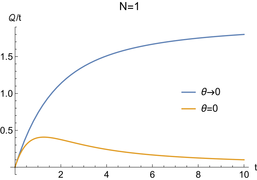
(a)

(b)

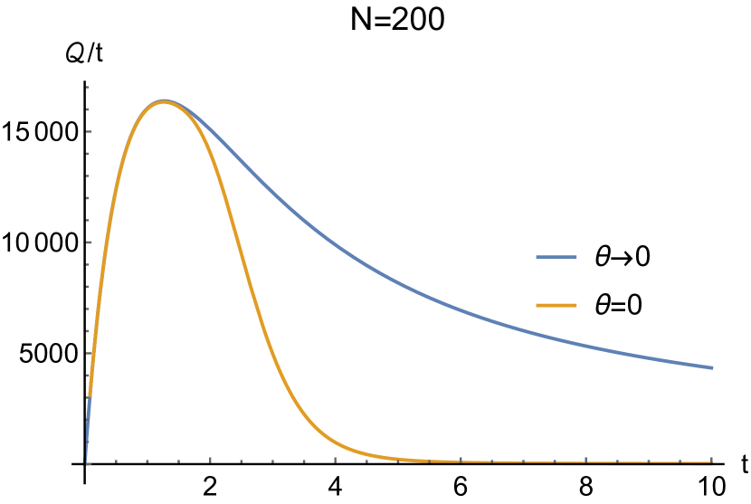
(c)

Figure 1: Plots of the QFI per unit time as a function of time, for $\kappa=1$, for different values of $N$.

References

References

- [1] Giovannetti V, Lloyd S and Maccone L 2011 Nat. Photonics 5 222–229 URL http://www.nature.com/articles/nphoton.2011.35
- [2] Helstrom C W 1976 Quantum detection and estimation theory (New York: Academic Press) ISBN 0123400503
- [3] Holevo A S 2011 Probabilistic and Statistical Aspects of Quantum Theory 2nd ed (Pisa: Edizioni della Normale) ISBN 978-88-7642-375-8 URL http://link.springer.com/10.1007/978-88-7642-378-9
- [4] Nagaoka H 1989 IEICE Tech. Rep. IT 89-42 9–14
- [5] Braunstein S L and Caves C M 1994 Phys. Rev. Lett. 72 3439–3443 URL https://link.aps.org/doi/10.1103/PhysRevLett.72.3439
- [6] Barndorff-Nielsen O E and Gill R D 2000 J. Phys. A 33 4481–4490 URL https://iopscience.iop.org/article/10.1088/0305-4470/33/24/306/
- [7] Paris M G A 2009 Int. J. Quantum Inf. 07 125–137 URL http://www.worldscientific.com/doi/abs/10.1142/S0219749909004839
- [8] Seveso L, Rossi M A C and Paris M G A 2017 Phys. Rev. A 95 012111 URL https://link.aps.org/doi/10.1103/PhysRevA.95.012111
- [9] Seveso L and Paris M G A 2018 Phys. Rev. A 98 032114 URL https://link.aps.org/doi/10.1103/PhysRevA.98.032114
- [10] Genoni M G, Duarte O S and Serafini A 2016 New J. Phys. 18 103040 URL https://iopscience.iop.org/article/10.1088/1367-2630/18/10/103040/
- [11] Haase J F, Smirne A, Huelga S F, Kołodyński J and Demkowicz-Dobrzański R 2018 Quantum Meas. Quantum Metrol. 5 13–39 URL http://www.degruyter.com/view/j/qmetro.2018.5.issue-1/qmetro-2018-0002/qmetro-2018-0002.xml
- [12] Šafránek D 2017 Phys. Rev. A 95 052320 URL http://link.aps.org/doi/10.1103/PhysRevA.95.052320
- [13] Šafránek D 2019 J. Phys. A 52 035304 URL https://iopscience.iop.org/article/10.1088/1751-8121/aaf068/
- [14] Serafini A 2017 Quantum continuous variables : a primer of theoretical methods (Boca Raton: CRC Press) ISBN 9781482246346
- [15] Cramér H 1946 Mathematical methods of statistics (Princeton: Princeton University Press) ISBN 0691005478
- [16] Bar-Shalom Y, Osborne R, Willett P and Daum F 2014 IEEE Trans. Aerosp. Electron. Syst. 50 2399–2405 URL http://ieeexplore.ieee.org/lpdocs/epic03/wrapper.htm?arnumber=6965787
- [17] Lu Q, Bar-Shalom Y, Willett P, Palmieri F and Daum F 2017 IEEE Trans. Aerosp. Electron. Syst. 53 2331–2343 URL http://ieeexplore.ieee.org/document/7894254/
- [18] Tsuda Y and Matsumoto K 2005 J. Phys. A 1593 URL http://iopscience.iop.org/0305-4470/38/7/014
- [19] Yang Y, Chiribella G and Hayashi M 2019 Commun. Math. Phys. 368 223–293 URL http://link.springer.com/10.1007/s00220-019-03433-4
- [20] Liu J, Jing X, Zhong W and Wang X 2014 Commun. Theor. Phys. 61 45–50
- [21] Suzuki J 2018 arXiv:1807.06990 URL https://arxiv.org/abs/1807.06990
- [22] Chernoff H 1954 Ann. Math. Stat. 25 573–578 URL http://projecteuclid.org/euclid.aoms/1177728725
- [23] Moran P A P 1971 Math. Proc. Cambridge Philos. Soc. 70 441 URL http://www.journals.cambridge.org/abstract{_}S0305004100050088
- [24] Self S G and Liang K y 1987 J. Am. Stat. Assoc. 82 605 URL https://www.jstor.org/stable/2289471
- [25] Andrews D W K 1999 Econometrica 67 1341–1383 URL http://doi.wiley.com/10.1111/1468-0262.00082
- [26] Davison A C 2003 Statistical models (Cambridge: Cambridge University Press) ISBN 9780511815850 URL http://ebooks.cambridge.org/ref/id/CBO9780511815850
- [27] Gill R D and Massar S 2000 Phys. Rev. A 61 042312 URL https://link.aps.org/doi/10.1103/PhysRevA.61.042312
- [28] Fujiwara A 2006 J. Phys. A 39 12489–12504 URL http://stacks.iop.org/0305-4470/39/i=40/a=014?key=crossref.8d5c19807e6293147953ec34b3d1075a
- [29] Gammelmark S and Mølmer K 2014 Phys. Rev. Lett. 112 170401 URL http://link.aps.org/doi/10.1103/PhysRevLett.112.170401
- [30] Albarelli F, Rossi M A C, Tamascelli D and Genoni M G 2018 Quantum 2 110 URL https://quantum-journal.org/papers/q-2018-12-03-110/
- [31] Albarelli F 2018 Continuous measurements and nonclassicality as resources for quantum technologies PhD thesis Università degli Studi di Milano
- [32] Brask J B, Chaves R and Kołodyński J 2015 Phys. Rev. X 5 031010 URL http://link.aps.org/doi/10.1103/PhysRevX.5.031010
- [33] Aolita L, Chaves R, Cavalcanti D, Acín A and Davidovich L 2008 Phys. Rev. Lett. 100 080501 URL https://link.aps.org/doi/10.1103/PhysRevLett.100.080501
- [34] Aolita L, Cavalcanti D, Acín A, Salles A, Tiersch M, Buchleitner A and de Melo F 2009 Phys. Rev. A 79 032322 URL https://link.aps.org/doi/10.1103/PhysRevA.79.032322
- [35] Chaves R, Brask J B, Markiewicz M, Kołodyński J and Acín A 2013 Phys. Rev. Lett. 111 120401 URL https://link.aps.org/doi/10.1103/PhysRevLett.111.120401
- [36] Zhong W, Sun Z, Ma J, Wang X and Nori F 2013 Phys. Rev. A 87 022337 URL http://link.aps.org/doi/10.1103/PhysRevA.87.022337