Model Risk in Credit Risk

R.FONTANA
 Department of Mathematical Sciences G. Lagrange,
Politecnico di Torino.
E. LUCIANO
 ESOMAS Department and Collegio Carlo Alberto, Università di Torino
P. SEMERARO
 Department of Mathematical Sciences G. Lagrange,
Politecnico di Torino
Elisa Luciano gratefully acknowledges financial support from the Italian Ministry of Education, University and Research (MIUR), ”Dipartimenti di Eccellenza” grant 2018-2022.Roberto Fontana and Patrizia Semeraro gratefully acknowledge financial support from the Italian Ministry of Education, University and Research (MIUR), ”Dipartimenti di Eccellenza” grant 2018-2022.
Abstract

The issue of model risk in default modeling has been known since inception of the Academic literature in the field. However, a rigorous treatment requires a description of all the possible models, and a measure of the distance between a single model and the alternatives, consistent with the applications. This is the purpose of the current paper. We first analytically describe all possible joint models for default, in the class of finite sequences of exchangeable Bernoulli random variables. We then measure how the model risk of choosing or calibrating one of them affects the portfolio loss from default, using two popular and economically sensible metrics, Value-at-Risk (VaR) and Expected Shortfall (ES).

keywords: Exchangeable Bernoulli distribution; risk measures; model risk.

1 Introduction

Models for default risk are prone to so-called model risk, in two senses: adopting the wrong model for the occurrence of default and calibrating or estimating a given model in a wrong way. The occurrence of model risk in the first sense is inherent in default, because of the difficulty of describing the causes of default or even of enumerating the determinants. Even the occurrence of calibration or estimation risk is overwhelming, because of the scarcity of observations, especially when looking at the joint default of specific obligors or particular categories of obligors, and lack of data to estimate parameters such as the correlation of defaults. The issue of model risk is indeed particularly strong in joint defaults, because on top of the model risk for marginal defaults there is model risk also in their joint distribution. We focus on joint modeling.

The issue of model risk in default modeling has been known since inception of the Academic literature in the field. Professionals are well aware of its importance too. However, a rigorous treatment requires a description of all the possible models and a measure of the distance between a single model and the alternatives, consistent with the applications. This is the purpose of the current paper. We first describe all possible joint models for default, in the class of exchangeable Bernoulli random variables. We then measure how the model risk of choosing or calibrating one of them affects the portfolio loss from default, using two popular and economically sensible metrics, Value-at-Risk (VaR) and Expected Shortfall (ES).

Univariate models of default belong to two families: structural and reduced-form models. The structural models, initiated by [1], reconduct default to the fact that the so-called asset value of a firm goes below a given monetary threshold. Reduced-form models, whose seminal work is due to [2], estimate from interest rates on defaultable debt the intensity of default, which is then interpreted as a fixed parameter or a stochastic process itself. For a survey of the approaches see for instance [3]. Multivariate models either make use of a copula to aggregate univariate default probabilities (see for instance [4], or [5], or use a Bernoulli mixture model (see chapter 8 in [6]).

The difficulties in choosing the right model for univariate modeling and calibrating it have been shown to be considerable. For structural models, the asset value is unobservable. For reduced-form models, rates of return on bonds are thought to include also a liquidity spread, which is difficult to separate from the default spread.

The difficulties in choosing or calibrating a multivariate model are even bigger (see the early recognition in [7]). Structural models can be calibrated, provided the correlation matrix of asset values can be. Multivariate reduced-form models are usually calibrated using the corresponding structural dependence (see chapter 10 in [5]).

The previous literature which assesses model risk in joint default usually takes as given the marginal probabilities of default, as we do: marginal default indicators are Bernoulli variables. It tries to explore the range of joint default probabilities, or the possible distribution of the loss from credit risk, which is the weighted sum of the marginal Bernoulli variables, where the weights are the exposures of the creditor towards different obligors. To do that, the literature uses different copulas (see[8]). Here we use the fact that all joint distributions or distributions of sums are generated starting from a finite number of so-called ray densities. Differently from copulas, all the rays can be found, either numerically or analytically.

[9] developed a simple method to represent all the Bernoulli variables with some specified moments, as a convex hull of densities belonging to the same class, the ray densities. They provide an algorithm to find the extreme rays of a given class without restrictions either on the number of variables or on the specified moments. The only drawback of the method is the amount of computational effort required for the numerical solution. The main contribution of the current paper consists in finding analytically the convex hull generators for the class of exchangeable Bernoulli variables with given mean and for the class of exchangeable Bernoulli variables with given mean and correlation. The analytical solution allows us to work in any dimension.

Once the multivariate Bernoulli variables represent the default indicators of a portfolio of obligors, the ray densities, that we can find analytically, allow us to describe all the joint distributions of defaults, even for large portfolios, and/or the possible distributions of the loss. There is a third mathematical contribution that helps in doing that: we show that the VaR bounds are reached on ray densities and we find an analytical expression for them. We also explicitly found bounds for the ES. We then measure the consequence of using a specific model (which might be ”wrong” one) or calibrating it in the ”wrong” way looking at the range of the possible VaR and ES.

So, the paper is novel both for the Mathematical contribution, namely the analytical description of the ray densities in high dimensions, and for the Mathematical Finance one, namely measurement of model risk using all possible multivariate distributions, obtained as linear convex combinations of generators that can be analytically found. This analytical solution allows us to find analogical bounds to measure model risk.

The paper unfolds as follows: Section 2 introduces the mathematical framework. Section 3 introduces the notion and properties of rays for exchangeable Bernoulli variables. Section 4 introduce the risk measures and provide analytical bounds for exchangeable Bernoulli variables. Model risk is discussed in Section 5. Section 5.1 provides calibrated examples. Section 6 concludes.

2
Default indicators: mathematical background

We consider a credit portfolio $P$ with $d$ obligors.

Some notation is needed. Let the random variable $\boldsymbol{X}=(X_{1},\ldots,X_{d})$ be the default indicators for the portfolio $P$ and let us assume that the indicator $\boldsymbol{X}$ is exchangeable, i.e. $\boldsymbol{X}\in\mathcal{E}_{d}$, where $\mathcal{E}_{d}$ is the class of $d$-dimensional exchangeable Bernoulli distributions. Let $\mathcal{E}_{d}(p)$ be the class of exchangeable Bernoulli distributions with the same Bernoulli marginal distributions $B(p)$, where $p$ is the marginal default probability of each obligor. If $\boldsymbol{X}=(X_{1},\dots,X_{d})$ is a random vector with joint distribution in $\mathcal{E}(p)$, we denote

  • its cumulative distribution function by $F_{p}$ and its probability mass function (pmf) by $f_{p}$;

  • the column vector which contains the values of $f_{p}$ over $\mathcal{X}_{d}:=\{0,1\}^{d}$, by $(f_{p}(\boldsymbol{x}):\boldsymbol{x}\in\mathcal{X}_{d})$ respectively; we make the non-restrictive hypothesis that the set $\mathcal{X}_{d}$ of $2^{d}$ binary vectors is ordered according to the reverse-lexicographical criterion. For example $\mathcal{X}_{2}=\{00,10,01,11\}$ and $\mathcal{X}_{3}=\{000,100,010,110,001,101,011,111\}$;

  • we denote by $\mathcal{P}_{d}$ the set of permutations on $\{1,\ldots,d\}$;

Recall that the expected value of $X_{i}$ is $p$, $\operatorname{E}[X_{i}]=p,\,\,\,i=1,\ldots,d$. We denote $q=1-p$. We assume that vectors are column vectors.

2.1 Exchangeable Bernoulli variables

Let us consider a pmf $f_{p}$ of a $d$-dimensional Bernoulli distribution with mean $p$. Since $f_{p}(\boldsymbol{x})=f_{p}(\sigma(\boldsymbol{x}))$ for any $\sigma\in\mathcal{P}_{d}$, any mass function $f_{p}$ in $\mathcal{E}_{d}(p)$ is given by $f_{i}:=f_{p}(\boldsymbol{x})$ if $\boldsymbol{x}=(x_{1},\ldots,x_{d})\in\mathcal{X}_{d}$ and $\#\{x_{j}:x_{j}=1\}=i$. Therefore we identify a mass function $f_{p}$ in $\mathcal{E}_{d}(p)$ with the corresponding vector $\boldsymbol{f}_{p}:=(f_{0},\ldots,f_{d})$. Furthermore, the moments depend only on their order, we therefore use $\mu_{{\alpha}}$ to denote a moment of order $\alpha=\text{ord}(\boldsymbol{\alpha})=\sum_{i=1}^{d}\alpha_{i}$, where $\boldsymbol{\alpha}\in\mathcal{X}_{d}$.

We also observe that the correlation $\rho$ between two Bernoulli variables $X_{i}\sim B(p)$ and $X_{j}\sim B(p)$ is related to the second-order moment $\mu_{2}=\operatorname{E}[X_{i}X_{j}]$ as follows

$$\mu_{2}=\rho pq+p^{2}.$$ (2.1)

2.2 Joint defaults, loss distribution and risk measures

To model the loss of a credit risk portfolio $P$ of $d$ obligors we consider the sum of the individual losses

$$L=\sum_{i=1}^{d}w_{i}X_{i},$$

where $w_{i}\in(0,1]$ and $\sum_{1=1}^{d}w_{i}=1$. In this paper we consider the case $w_{i}=\frac{1}{d},\,i\in\{1,\ldots,d\}$. The extension to unequal weights can be done numerically. For equal weights, $L=\frac{S_{d}}{d}$, where

$$S_{d}=\sum_{i=1}^{d}X_{i}$$

represents the number of defaults. Therefore, the distribution of $S_{d}$ represents the distribution of the loss. Since the vector of default indicators $\boldsymbol{X}$ is assumed to be exchangeable, there is a one-to-one correspondence between the distribution of the number of defaults and the joint distribution of $\boldsymbol{X}$. In fact, as said in the preliminaries, since $f_{p}(\boldsymbol{x})=f_{p}(\sigma(\boldsymbol{x}))$ for any $\sigma\in\mathcal{P}_{d}$, any mass function $f_{p}$ in $\mathcal{E}_{d}(p)$ is given by $f_{i}:=f_{p}(\boldsymbol{x})$ if $\boldsymbol{x}=(x_{1},\ldots,x_{d})\in\mathcal{D}_{d}$ and $\#\{x_{j}:x_{j}=1\}=i$. We can define a one-to-one correspondence between $\mathcal{E}_{d}(p)$ and the class of the distributions on the number of defaults.

Let $\mathcal{S}_{d}(p)$ be the class of distributions $p_{S}$ on $\{0,\ldots,d\}$ such that $S_{d}=\sum_{i=0}^{d}X_{i}$ with $\boldsymbol{X}\in\mathcal{E}_{d}(p)$. Let $p_{S}(j)=p_{j}=P(S_{d}=j)$ and $\boldsymbol{p}_{S}=(p_{0},\ldots,p_{d})$.

The map:

$$\begin{split}E:\mathcal{E}_{d}(p)&\rightarrow\mathcal{S}_{d}(p)\\ f_{j}&\rightarrow p_{j}={\binom{d}{j}}f_{j}.\end{split}$$ (2.2)

is a one-to-one correspondence between $\mathcal{E}_{d}(p)$ and $\mathcal{S}_{d}(p)$. Therefore we have

$$\begin{split}\mathcal{E}_{d}(p)&\leftrightarrow\mathcal{S}_{d}(p)\end{split}$$ (2.3)

We now prove that the class of distributions $\mathcal{S}_{d}(p)$ coincides with the entire class of discrete distributions with mean $dp$, say $\mathcal{D}_{d}(dp)$. This fact is useful to simplify the search of the generators of $\mathcal{E}_{d}(p)$. The class $\mathcal{D}_{d}(dp)$ is not of special interest in this context, but it is introduced for technical reasons.

Proposition 2.1.

It holds $\mathcal{S}_{d}(p)=\mathcal{D}_{d}(dp)$.

Proof.

1) $\mathcal{S}_{d}(p)\subseteq\mathcal{D}_{d}(dp)$. This is trivial.

2) $\mathcal{D}_{d}(dp)\subseteq\mathcal{S}_{d}(p)$. Let $\{p_{0},\ldots,p_{d}\}\in\mathcal{D}_{d}(dp)$. Let us define $f_{i}=\frac{p_{i}}{\binom{d}{j}}$ and $p(x_{1},\ldots,x_{d})=f_{i}$ for all $(x_{1},\ldots,x_{d})$ such that $\sum_{j=0}^{d}x_{j}=i$. The mass function $p$ is the mass function of a $d$-dimensional Bernoulli random vector, which is exchangeabe by contruction. We have

$$\begin{split}E[X_{1}]&=P(X_{1}=1)=\sum_{(x_{1},\ldots,x_{d}):x_{1}=1}p(x_{1},\ldots,x_{d})=\sum_{i=1}^{d}\sum_{\begin{subarray}{c}(x_{1},\ldots,x_{d}):x_{1}=1,\\ \sum_{i=0}^{d}x_{i}=1\end{subarray}}p(x_{1},\ldots,x_{d})\\ &=\sum_{i=1}^{d}\sum_{\begin{subarray}{c}(x_{1},\ldots,x_{d}):x_{1}=1,\\ \sum_{i=0}^{d}x_{i}=1\end{subarray}}f_{i}=\sum_{i=1}^{d}\binom{d-1}{i-1}\frac{p_{i}}{\binom{d}{i}}\\ &=\sum_{i=1}^{d}\frac{(d-1)!}{(i-1)!(d-1-i+1)!}\frac{i!(d-i)!}{d!}p_{i}\\ &=\sum_{i=1}^{d}\frac{i}{d}p_{i}=\frac{1}{d}pd=p.\end{split}$$ (2.4)

Then $\boldsymbol{X}\in\mathcal{E}_{d}(p)$.

Now let $S_{d}:=\sum_{i=1}^{d}X_{i}$. We have $P(S_{d}=j)=\binom{d}{j}f_{j}=p_{j}$ and $\{p_{0},\ldots,,p_{d}\}\in\mathcal{S}_{d}(p)$.

Therefore the three classes $\mathcal{E}_{d}(p)$, $\mathcal{S}_{d}(p)$ and $\mathcal{D}_{d}(dp)$ are essentially the same class, i.e.

$$\begin{split}\mathcal{E}_{d}(p)&\leftrightarrow\mathcal{S}_{d}(p)\equiv\mathcal{D}_{d}(dp)\end{split}$$ (2.5)

Thanks to the above proposition to find the generators of $\mathcal{S}_{d}(p)$ we can look for the generators of $\mathcal{D}_{d}(dp)$. This simplifies the search. The generators we find are in one-to-one relationship with the generators of $\mathcal{E}_{d}(p)$.

3 Exchangeable Bernoulli generators

We build on the results in [9], where the authors represent the Fréchet class of multivariate $d$-dimensional Bernoulli distributions with given margins and/or pre-specified moments as the points of a convex hull. The generators of the convex hull are mass functions in the class and they can be explicitly found. The range of application of this method is limited only by the computational effort required since the number of generators increases very quickly as the dimension increases. We show here that under the condition of exchangeability this limit can be overtaken because we analytically find the ray densities. As a consequence the dimension is no longer an issue. We focus on two classes: the class $\mathcal{E}_{d}(p)$ and the class $\mathcal{E}_{d}(p,\rho)$, i.e. the class of exchangeable Bernoulli vectors with given $p$ and given correlation $\rho$. The one to one correspondence $E$ between the distributions $\boldsymbol{p}_{S}\in\mathcal{S}_{d}(p)$ and $\boldsymbol{f}_{p}\in\mathcal{E}_{d}(p)$ is also a one-to-one correspondence between the distributions $\boldsymbol{p}_{S}\in\mathcal{S}_{d}(p,\rho)$ and $\boldsymbol{f}_{p}\in\mathcal{E}_{d}(p,\rho)$.

In Section 3.1 we represent the class $\mathcal{E}_{d}(p)$ as a convex hull of mass functions in the class, which we call ray densities, so that each mass function is a convex combinations of ray densities belonging to $\mathcal{E}_{d}(p)$. We analytically find the ray densities and their number, that depends on the dimension $d$ and the mean value $p$. The one-to-one map between $\mathcal{E}_{d}(p)$ and $\mathcal{S}_{d}(p)$ and Proposition 2.1 are crucial.

In Section 3.2 we represent the class $\mathcal{E}_{d}(p,\rho)$, as well as $\mathcal{S}_{d}(p,\rho),$ as a convex hull of ray densities. We analyticall find them using the one-to-one correspondence between the class $\mathcal{E}_{d}(p)$ and the class $\mathcal{S}_{d}(p)$ and between the relative subclasses $\mathcal{S}_{d}(p,\rho)$ and $\mathcal{E}_{d}(p,\rho)$. We prove that ray densities in $\mathcal{S}_{d}(p,\rho)$ have support on at most three points. By so doing, also in this case the dimension $d$ is not an issue.

3.1 For given marginal default probabilities

Using the equivalence $\mathcal{S}_{d}(p)\equiv\mathcal{D}_{d}(pd)$ stated in Proposition 2.1 a pmf in $\mathcal{S}_{d}(p)$ is a pmf on $\{0,\ldots,d\}$ with mean $pd$. Thanks to the map $E$ in Equation 2.5 this is also equivalent to find a set of conditions that a pmf of a multivariate Bernoulli has to satisfy for being in $\mathcal{E}_{d}(p)$. This fact is crucial in the following proposition.

Proposition 3.1.

Let $\boldsymbol{Y}$ be a discrete random variable defined over $\{0,\ldots,d\}$ and let $p_{Y}$ be its pmf. Then

$$Y\in\mathcal{S}_{d}(p)\,\,\,\Longleftrightarrow\,\,\,\sum_{j=0}^{d}(j-pd)p_{Y}(j)=0.$$ (3.1)
Proof.

Let $\boldsymbol{Y}$ be a discrete random variable defined over $\{0,\ldots,d\}$. By Proposition 2.1 $Y\in\mathcal{S}_{d}(p)$ iff $E[Y]=pd$. It holds

$$E[Y]=pd\Longleftrightarrow E[Y-pd]=0\Longleftrightarrow\sum_{j=0}^{d}(j-pd)p_{Y}(j)=0.$$

Using Proposition 3.1 we can find all generators of $\mathcal{S}_{d}(p)$ that, thanks to the map $E$ is equivalent to find all the generators of $\mathcal{E}_{d}(p)$.

We have to find the solutions $\boldsymbol{p}_{S}=(p_{0},\ldots,p_{j})$ of

$$\sum_{j=0}^{d}(j-pd)p_{j}=0.$$ (3.2)

with the conditions $p_{j}\geq 0,\,j=0,\ldots,d$ and $\sum_{j=0}^{d}p_{j}=1$. From the standard theory of linear equations we know that all the positive solutions of 3.2 are elements of the convex cone

$$\mathcal{C}_{p}=\{\boldsymbol{z}\in\mathbb{R}^{d+1}:\sum_{j=0}^{d}a_{j}z_{j}=0,\,I\boldsymbol{z}\geq 0\},$$ (3.3)

where $a_{j}=j-pd$ and $I$ is the $(d+1)\times(d+1)$ identity matrix, and therefore can be generated as convex combinations of a set of generators which are referred to as extremal rays of the linear system. The proof of the following proposition follows Lemma 2.3 in [10].

Proposition 3.2.

Let us consider the linear system

$$A\boldsymbol{z}=0,\boldsymbol{z}\in\mathbb{R}^{d+1}$$ (3.4)

where $A$ is a $m\times(d+1)$ matrix, $m\leq d$ and $\operatorname{rank}A=m$. The extremal rays of the system 3.4 have at most $m+1$ non-zero components.

Proof.

Let $\mathcal{C}_{A}=\{\boldsymbol{z}\in\mathbb{R}^{d+1}:A\boldsymbol{z}=0,\,I\boldsymbol{z}\geq 0\}$ be the convex cone of all the positive solutions of 3.4. A solution $\boldsymbol{r}$ of 3.2 is an extremal ray of $\mathcal{C}_{A}$ iff $I^{*}\boldsymbol{z}=0$ for a submatrix $n_{I^{*}}\times(d+1)$, $I^{*}$ of $I$ and

$$\text{rank}\left[\begin{split}&A\\ &I^{*}\end{split}\right]=d.$$ (3.5)

Therefore $\operatorname{rank}I^{*}\geq d-m$ and $\boldsymbol{r}$ has at most $(d+1)-(d-m)=m+1$ non-zero components. ∎

Corollary 3.1.

The extremal rays of the convex cone $\mathcal{C}_{p}$ in 3.3 have at most two non-zero components.

Proof.

Let $a_{j}=j-pd$, $j=0,\ldots,d$. The matrix $A=[a_{0},\ldots,a_{d}]$ is the row vector of the coefficients. Since $\operatorname{rank}A=m=1$ then an extremal ray $\boldsymbol{r}$ has at most two non-zero components. ∎

Proposition 3.3.

The extremal rays of of the convex cone $\mathcal{C}_{p}$ in 3.3 are

$$p_{j_{1},j_{2}}(y)=\left\{\begin{array}[]{cc}\frac{j_{2}-pd}{j_{2}-j_{1}}&y=j_{1}\\ \frac{pd-j_{1}}{j_{2}-j_{1}}&y=j_{2}\\ 0&\text{otherwise}\end{array}\right.,$$ (3.6)

with $j_{1}=0,1,\ldots,j_{1}^{M}$, $j_{2}=j_{2}^{m},j_{2}^{m}+1,\ldots,d$, $j_{1}^{M}$ is the largest integer less that $pd$ and $j_{2}^{m}$ is the smallest integer greater than pd.

If $pd$ is integer the extremal rays contain also

$$p_{pd}(y)=\left\{\begin{array}[]{cc}1&y=pd\\ 0&\text{otherwise}\end{array}\right..$$ (3.7)
Proof.

Let $a_{j}=j-pd$. Equation 3.2 becomes

$$\sum_{j=0}^{d}a_{j}p_{j}=0.$$ (3.8)

By Corollary 3.1 the extremal rays have at most two non zero components, say $j_{1},j_{2}$. Therefore the extremal rays can be found considering the equations

$$a_{j_{1}}p_{j_{1}}+a_{j_{2}}p_{j_{2}}=0,$$ (3.9)

where we make the non restrictive assumption $j_{1}<j_{2}$. The equation 3.2 has positive solutions only if $a_{j_{1}}a_{j_{2}}<0$. We observe that $a_{j_{1}}<0$ for $0\leq j_{1}\leq j_{1}^{M}$ where $j_{1}^{M}$ is the largest integer less than $pd$ and $a_{j_{2}}>0$ for $j_{2}^{m}\leq j_{2}\leq d$ where $j_{2}^{m}$ is the smallest integer greater than $pd$. In this case we have $j_{2}^{m}=j_{1}^{M}+1$. It follows that for $0\leq j_{1}\leq j_{1}^{M}$ and $j_{2}^{m}\leq j_{2}\leq d$ we have $a_{j_{1}}a_{j_{2}}<0$. A positive solution of Equation 3.2 is

$$\left\{\begin{array}[]{c}\tilde{p}_{y}(j_{1})=x_{j_{1}}=j_{2}-pd\\ \tilde{p}_{y}(j_{2})=-x_{j_{2}}=pd-j_{1}\end{array}\right..$$ (3.10)

We have $\tilde{p}_{y}(j_{1})+\tilde{p}_{y}(j_{2})=j_{2}-pd+pd-j_{1}=j_{2}-j_{1}$ and then the normalized extremal rays corresponding to $j_{1}$ and $j_{2}$ are given by (3.6). If $pd$ is integer we have $a_{pd}=0$. It follows that (3.7) is also an extremal solution.

We denote by $R_{(j_{1},j_{2})}$ and $R_{pd}$ the random variables whose pmf are $\boldsymbol{r}_{(j_{1},j_{2})}$ and $\boldsymbol{r}_{pf}$ respectively. We will refer to $\boldsymbol{r}_{(j_{1},j_{2})}$ and $\boldsymbol{r}_{pf}$ as ray densities and $R_{(j_{1},j_{2})}$ and $R_{pd}$ as ray random variables. Notice that $\boldsymbol{r}_{(0,d)}=(1-p,0,\ldots,0,p)$.

Corollary 3.2.

If $pd$ not integer there are $n_{p}=(j_{1}^{m}+1)(d-j_{1}^{m})$ ray densities.

If $pd$ integer there are $n_{p}=d^{2}p(1-p)+1$ ray densities.

We have proved the following.

Theorem 3.1.

The following holds. $S_{d}\in\mathcal{S}_{d}(p)$ iff there exist $\lambda_{1},\ldots,\lambda_{n_{p}}\geq 0$ summing up to 1 such that

$$\boldsymbol{p}_{S}=\sum_{i=1}^{n_{p}}\lambda_{i}\boldsymbol{r}_{i},$$ (3.11)

where $\boldsymbol{r}_{i}$ are the ray densities and $n_{p}$ is the number of ray densities.

3.1.1 Second order moments

Let $\boldsymbol{X}\in\mathcal{E}_{d}(p)$ and let $\mu_{2}=E[X_{i}X_{j}]$ its second order cross moment.

Proposition 3.4.

Let $\boldsymbol{X}\in\mathcal{E}_{d}(p)$. It holds

$$\mu_{2}=\sum_{k=0}^{d}\frac{k(k-1)}{d(d-1)}p_{k}.$$ (3.12)
Proof.

By exchangeability we can fix any pair $i,j\in\{1,\ldots,d\}$. It holds

$$\begin{split}\mu_{2}=P(X_{i}=1,X_{j}=1)&=\sum_{k=0}^{d}P(X_{i}=1,X_{j}=1|S_{d}=k)P(S_{d}=k)\\ &=\sum_{k=2}^{d}\frac{\binom{d-2}{k-2}}{\binom{d}{k}}p_{k}=\sum_{k=2}^{d}\frac{k(k-1)}{d(d-1)}p_{k}\\ &=\sum_{k=0}^{d}\frac{k(k-1)}{d(d-1)}p_{k},\end{split}$$

Thanks to the one-to-one map $E$ we can find the bounds for the second order moments of $\mathcal{E}_{d}(p)$ using the second order moments of $S_{d}$. We have

$$E[S_{d}^{2}]=E[(X_{1}+\ldots+X_{d})^{2}]=pd+d(d-1)\mu_{2}.$$ (3.13)
Proposition 3.5.

Let $\boldsymbol{X}\in\mathcal{E}_{d}(p)$. Then if $pd$ is not integer

$$\frac{1}{d(d-1)}[-j_{1}^{m}(j_{1}^{m}+1)+2j_{1}^{m}pd]\leq\mu_{2}\leq p.$$ (3.14)

If $pd$ is integer

$$\frac{p(pd-1)}{(d-1)}\leq\mu_{2}\leq p.$$ (3.15)
Proof.

From (3.13) we have $\mu_{2}=\frac{1}{d(d-1)}[E[S^{2}_{d}]-pd]$. Since $S_{d}\in\mathcal{S}_{d}(p)$ its density is a convex linear combinations of the ray densities. It is known that the moments of $S_{d}$ are moments of the ray variables. We obtain

$$E[R_{(j_{1},j_{2})}^{2}]=j_{1}^{2}\frac{j_{2}-pd}{j_{2}-j_{1}}+j_{2}^{2}\frac{j_{2}-pd}{pd-j_{1}}=-j_{1}j_{2}+(j_{1}+j_{2})pd,$$ (3.16)

and

$$E[R_{pd}^{2}]=(pd)^{2}.$$ (3.17)

To maximize $\mu_{2}$ we have to maximize $E[S_{d}^{2}]$. From (3.16) and (3.17) we easily get that the ray variable for which the second order moment is maximum is $R_{(0,d)}$ and we have $E[R_{(0,d)}^{2}]=(pd)^{2}$. Then, after some computations, $\mu_{2}^{M}=p$.

To minimize $\mu_{2}$ we have to minimize $E[S_{d}^{2}]$. We consider two cases.

If $pd$ is not integer, from (3.16) we have that the ray variable for which the second order moment is minimum is $R_{(j_{1}^{M},j_{2}^{m})}=R_{(j_{1}^{M},j_{1}^{M}+1)}$, for which we have $E[R_{(j_{1}^{M},j_{1}^{M}+1)}^{2}]=-j_{1}^{m}(j_{1}^{m}+1)+(2j_{1}^{m}+1)pd$ and the assert follows.

If $pd$ is integer the ray variable for which the second order moment is minimum is $R_{pd}$. Since $E[R_{pd}^{2}]=(pd)^{2}$, (3.15) follows.

Thanks to equation (2.1), the next corollary to the above proposition provides bounds for the correlation coefficient.

Corollary 3.3.

Let $\boldsymbol{X}\in\mathcal{E}_{d}(p)$. Then if $pd$ is not integer

$$\frac{\frac{1}{d(d-1)}[-j_{1}^{m}(j_{1}^{m}+1)+2j_{1}^{m}pd]-p^{2}}{p(1-p)}\leq\rho\leq 1.$$ (3.18)

If $pd$ is integer

$$-\frac{1}{d-1}\leq\rho\leq 1.$$ (3.19)

3.2 For given marginal default probabilities and default correlations

In this section we consider the class of multivariate exchangeable Bernoulli mass functions with given margins $p$ and given correlation $\rho$, i.e. the class $\mathcal{E}_{d}(p,\rho)$. We now find the generators of $\mathcal{S}_{d}(p,\rho)$.

Since $S\in\mathcal{S}_{d}(p,\rho)$ iff $E[S_{d}]=pd$ and $E[S_{d}^{2}]=dp+d(d-1)\mu_{2}$, we can define an homogeneous linear system whose solutions are the pmf in $\mathcal{S}_{d}(p,\rho)$.

Proposition 3.6.

The following holds. $S_{d}\in\mathcal{S}_{d}(p,\rho)$ iff there exist $\lambda_{1},\ldots,\lambda_{n_{p}}\geq 0$ summing up to 1 such that

$$\boldsymbol{p}_{S}=\sum_{i=1}^{n_{p}}\lambda_{i}\boldsymbol{r}_{\rho,i},$$ (3.20)

where $\boldsymbol{r}_{\rho,i}$ are the normalized extremal rays of the cone $\mathcal{C}_{p,\rho}$ defined by linear system:

$$\left\{\begin{array}[]{c}\sum_{j=0}^{d}[{j}-pd]p_{j}=0\\ \sum_{j=0}^{d}[j^{2}-(pd+d(d-1)\mu_{2})]p_{j}=0.\end{array}\right.$$ (3.21)

The following corollary of Proposition 3.2 characterizes the ray densities of $\mathcal{S}_{d}(p,\rho)$.

Corollary 3.4.

The extremal rays of $\mathcal{S}_{d}(p,\rho)$ have support on at most three points.

Proof.

The extremal rays of (3.2) are the normalized extremal rays of the convex cone $\mathcal{C}=\{\boldsymbol{z}\in\mathbb{R}^{d+1}:A\boldsymbol{z}=0,\,I\boldsymbol{z}\geq 0\}$, where $A$ is the matrix coefficients of (3.21). We have $\operatorname{rank}A\leq 2$. From Proposition 3.2 it follows $\text{rank}(\boldsymbol{I}^{*})=d-3,\,d-2,\,d-1$ and $\boldsymbol{I}^{*}=(e_{3},\ldots,e_{n})^{T}$ to let $\boldsymbol{A}|\boldsymbol{I}$ have $d-1$ independent rows. Since $\boldsymbol{I}^{*}\boldsymbol{R}=0$, if $\text{rank}(\boldsymbol{I}^{*})=d-3$, $\boldsymbol{R}$ has only three non zero components, if $\text{rank}(\boldsymbol{I}^{*})=d-2$, $\boldsymbol{R}$ has only two non zero components, and if $\text{rank}(\boldsymbol{I}^{*})=d-1$, $\boldsymbol{R}$ has only one non zero component. In the latter case all the mass is one point.

Proposition 3.7.

The extremal rays of (3.2) are $\boldsymbol{r}_{\rho}=(p_{0},\ldots,p_{d})$, where $p_{l}=0,l\neq i,j,k$,

$$\begin{split}&p_{i}=\frac{jk-(j+k-1)dp+d(d-1)\mu_{2}}{(k-i)(j-i)}\\ &p_{j}=-\frac{ik-(i+k-1)dp+d(d-1)\mu_{2}}{(k-j)(j-i)}\\ &p_{k}=\frac{ij-(i+j-1)dp+d(d-1)\mu_{2}}{(k-j)(k-i)},\\ \end{split}$$ (3.22)

with $i<j<k$ and $p_{i},p_{j},p_{k}\geq 0$

Proof.

The extremal rays of (3.2) can be found as follows. Let $\alpha_{j}:=j-pd$ and $\beta_{j}:=j^{2}-(pd+d(d-1)\mu_{2})$, we can write system (3.21) as follows:

$$\left\{\begin{array}[]{c}\sum_{j=0}^{d}\alpha_{j}p_{j}=0\\ \sum_{j=0}^{d}\beta_{j}p_{j}=0,\end{array}\right.$$ (3.23)

Let now $A=\begin{bmatrix}\alpha_{0}&\ldots&\alpha_{d}\\ \beta_{0}&\ldots&\beta_{d}\end{bmatrix}$. From Corollary 3.4 we have to find the positive solutions $(z_{j},z_{j},z_{k})$, for $i<j<k$ , of

$$\left\{\begin{array}[]{c}\alpha_{i}x_{i}+\alpha_{j}x_{j}+\alpha_{k}x_{k}=0\\ \beta_{i}x_{i}+\beta_{j}x_{j}+\beta_{k}x_{k}=0,\end{array}\right.$$ (3.24)

Then, from a positive solution, we find $p_{l}=\frac{z_{l}}{z_{i}+z_{j}+z_{k}}$, $l\in\{i,j,k\}$.

Letting $x_{k}=1$ the system 3.25 becomes

$$\left\{\begin{array}[]{c}\alpha_{i}x_{i}+\alpha_{j}x_{j}=-\alpha_{k}\\ \beta_{i}x_{i}+\beta_{j}x_{j}=-\beta_{k},\end{array}\right.$$ (3.25)

and its solution can be determined by standard computation using Cramer’s formula. ∎

We conclude this section with the following proposition that gives necessary and sufficient conditions for a ray density in $\mathcal{S}_{d}(p)$ to be also a ray density in $\mathcal{S}_{d}(p,\rho)$ .

Proposition 3.8.

A ray density $\boldsymbol{r}\in\mathcal{S}_{d}(p,\rho)$ has support on two points iff it is a ray density in $\mathcal{S}_{d}(p)$ and $\mu_{2}^{\boldsymbol{r}}=\mu_{2}$, where $\mu_{2}^{\boldsymbol{r}}$ is the second order cross moment of $\boldsymbol{r}$.

Proof.

If $\boldsymbol{r}$ is a solution of (3.21) it is also a solution of (3.2) and since it has support of two poins by assumption it is an extremal solution. Thus $\boldsymbol{r}\in\mathcal{S}_{d}(p)$ is a ray density. Viceversa if $\boldsymbol{r}\in\mathcal{S}_{d}(p)$ it satisfies the first equation of (3.21) by definition and if $\mu_{2}^{\boldsymbol{r}}=\mu_{2}$ it also satisfy the second equation by construction. Since it has mass on two points it is an extremal solution of (3.21). ∎

4 Financial risk measures and their bounds

As measures of portfolio risk we consider the value at risk (VaR) and the expected shortfall (ES) of $S_{d}$. We recall their definition for a general random variable $Y$.

Definition 4.1.

Let $Y$ be a random variable representing a loss with finite mean. Then the $\text{VaR}_{\alpha}$ at level $\alpha$ is defined by

$$\text{VaR}_{\alpha}(Y)=\inf\{y\in\mathbb{R}:P(Y\leq y)\geq\alpha\}$$ (4.1)

and the expected shortfall at level $\alpha$ is defined by

$$\text{ES}_{\alpha}(Y)=E[Y|Y\geq Var_{\alpha}(Y)]$$ (4.2)

The following proposition provides the bounds for the $\text{VaR}_{\alpha}$ and $\text{ES}_{\alpha}$ of $S_{d}$, for $S_{d}$ in a given class.

Proposition 4.1.
  1. 1.

    Let $S_{d}\in\mathcal{S}_{d}(p)[\mathcal{S}_{d}(p,\rho)]$ and let $\text{VaR}_{\alpha}(S_{d})$ be its value at risk. Then

    $$\min_{R}\text{VaR}_{\alpha}(R)\leq\text{VaR}_{\alpha}(S_{d})\leq\max_{R}\text{VaR}_{\alpha}(R),$$

    where $R$ are the ray densities of $\mathcal{S}_{d}(p)[\mathcal{S}_{d}(p,\rho)]$.

  2. 2.

    Let $S_{d}\in\mathcal{S}_{d}(p)[\mathcal{S}_{d}(p,\rho)]$ and let $ES_{\alpha}(S_{d})$ be its expected shortfall. Then

    $$\min_{R}\text{VaR}_{\alpha}(R)\leq\text{ES}_{\alpha}(S_{d})\leq d,$$

    where $R$ are the ray densities of $\mathcal{S}_{d}(p)[\mathcal{S}_{d}(p,\rho)]$.

Proof.
  1. 1.

    Let $\tau_{S}=\text{VaR}_{\alpha}(S_{d})=inf\{y\in\boldsymbol{\Theta}:P(S_{d}\leq y)\geq\alpha\}$. Let $\tau_{i}=\text{VaR}_{\alpha}(R_{i})$, $\tau_{M}=\max_{i}\tau_{i}$ and $\tau_{m}=\min_{i}\tau_{i}$. It holds

    $$\begin{split}P(S_{d}\leq\tau_{M})&=\sum_{y\leq t_{M}}p_{S}(y)=\sum_{y\leq t_{M}}\sum_{i=1}^{n_{p}}\lambda_{i}p_{R_{i}}(y)\\ &=\sum_{i=1}^{n_{p}}\lambda_{i}\sum_{y\leq t_{M}}p_{R_{i}}(y)\geq\sum_{i=1}^{n_{p}}\lambda_{i}\alpha=\alpha,\end{split}$$ (4.3)

    thus $\tau_{S}\leq\tau_{M}$. It holds

    $$\begin{split}P(S_{d}\leq\tau_{m})&=\sum_{i=1}^{n_{p}}\lambda_{i}\sum_{y\leq t_{m}}p_{R_{i}}(y)=\sum_{i=1}^{n_{p}}\lambda_{i}\beta_{i},\end{split}$$ (4.4)

    with $\beta_{i}\leq\alpha$ therefore we have $P(S_{d}\leq\tau_{m})\leq\alpha$. Thus $\tau_{S}\geq\tau_{m}$ and $\tau_{m}\leq\tau_{S}\leq\tau_{M}$.

  2. 2.

    $ES_{\alpha}\geq\tau_{m}$ and $ES_{\alpha}\leq d$ are trivial.

The above propositions shows that $\text{VaR}_{\alpha}$ reaches the maximum and minimum values in $\mathcal{S}_{d}(p)$ [$\mathcal{S}_{d}(p,\rho)$] on the ray densities and therefore we are able to explicitly find them.

Remark 1.

The bounds for $ES_{\alpha}$ are weaker and trivial. Nevertheless, at least in some cases, they cannot be improved. In fact, consider the ray density $\boldsymbol{r}=(1-p,\ldots,p)\in\mathcal{E}_{d}(p)$. If $1-p\leq\alpha$ then $ES_{\alpha}=d$. As a consequence for marginal default probabilities higher then $1-\alpha$ the bound is reached.

Thanks to Proposition 3.3 that gives the analytical expression of the ray densities of $\mathcal{S}_{d}(p)$, the following proposition provides the analytical bounds for $\text{VaR}_{\alpha}$ in $\mathcal{S}_{d}(p)$.

Proposition 4.2.

Let us consider the class $\mathcal{S}_{d}(p)$ and let $j_{1}^{p}=\frac{(p-(1-\alpha))d}{\alpha}$.

  1. 1.

    If $j_{1}^{p}<0$, $\min\text{VaR}_{\alpha}(R_{(j_{1},j_{2})})=0$ and $\max\text{VaR}_{\alpha}(R_{(j_{1},j_{2})})=j_{2}^{*}$, where $j_{2}^{*}$ is the largest integer smaller than $\frac{pd}{1-\alpha}$.

  2. 2.

    If $0\leq j_{1}^{p}\leq j_{1}^{M}$, $\min\text{VaR}_{\alpha}(R_{(j_{1},j_{2})})=j_{1}^{*}$, where $j_{1}^{*}$ is the smallest integer greater or equal to $j_{1}^{p}$ and $\max\text{VaR}_{\alpha}(R_{(j_{1},j_{2})})=d$.

  3. 3.

    If $j_{1}^{p}>j_{1}^{M}$, $\min\text{VaR}_{\alpha}(R_{(j_{1},j_{2})})=j_{2}^{m}=j_{1}^{M}+1$ and $\max\text{VaR}_{\alpha}(R_{(j_{1},j_{2})})=d$. In this case, if $pd$ is integer $j_{1}^{M}+1=pd$.

Proof.

Let us consider first the case $pd$ not integer. The ray densities are given in (3.6) with $0\leq j_{1}\leq j_{1}^{M}$ and $j_{1}^{M}+1\leq j_{2}\leq d$. From the definition of $VaR$ we have

$$\text{VaR}_{\alpha}(R_{(j_{1},j_{2})})=j_{1}\Longleftrightarrow\boldsymbol{r}_{(j_{1},j_{2})}(j_{1})\geq\alpha.$$ (4.5)

It follows

$$\begin{split}&\boldsymbol{r}_{(j_{1},j_{2})}(j_{1})=\frac{j_{2}-pd}{j_{2}-j_{1}}\geq\alpha,\\ \end{split}$$ (4.6)

then

$$\begin{split}&{j_{2}}\geq-\frac{\alpha}{1-\alpha}{j_{1}}+\frac{pd}{1-\alpha}.\end{split}$$ (4.7)

We also know that $j_{2}\leq d$, so let us determine the point $P$ of intersection of ${j_{2}}=-\frac{\alpha}{1-\alpha}{j_{1}}+\frac{pd}{1-\alpha}$ and $j_{2}=d$. The solution of

$$\left\{\begin{array}[]{l}{j_{2}}=-\frac{\alpha}{1-\alpha}{j_{1}}+\frac{pd}{1-\alpha}\\ j_{2}=d\end{array}\right.$$ (4.8)

is $P=(j_{1}^{P},j_{2}^{P})=(\frac{(p-(1-\alpha))d}{\alpha},d)$. We distinguish three cases, depending on $j_{1}^{P}$.

  1. 1.

    $j_{1}^{p}<0$. In this case it will follow that $\text{VaR}_{\alpha}(R_{(0,j_{2})})=0$ for all $\frac{pd}{1-\alpha}<j_{2}\leq d$ and then the minimum value of $\text{VaR}_{\alpha}(R_{(j_{1},j_{2})})=0$. With respect to the maximum value of $\text{VaR}_{\alpha}(R_{(j_{1},j_{2})})$ it will be obtained by $\text{VaR}_{\alpha}(R_{(0,j_{2}^{*})})$, where $j_{2}^{*}$ is the largest integer smaller than $\frac{pd}{1-\alpha}$.

  2. 2.

    $0\leq j_{1}^{p}\leq j_{1}^{M}$. Let us define $j_{1}^{*}$ as the smallest integer greater or equal to $j_{1}^{P}$. It follows that $\text{VaR}_{\alpha}(R_{(j_{1}^{*},j_{2})})=j_{1}^{*}$, $j_{2}^{*}<j_{2}\leq d$ with $j_{2}^{*}$ is the smallest integer greater or equal to $-\frac{\alpha}{1-\alpha}{j_{1}^{*}}+\frac{pd}{1-\alpha}$. Then the minimum value of $VaR_{\alpha}(R_{(j_{1},j_{2})})=j_{1}^{*}$. The maximum value of $\text{VaR}_{\alpha}(R_{(j_{1},j_{2})})$ is $d$.

  3. 3.

    $j_{1}^{p}>j_{1}^{M}$. In this case $\text{VaR}_{\alpha}(R_{(j_{1},j_{2})})=j_{2}$. Then the minimum value of $\text{VaR}_{\alpha}(R_{(j_{1},j_{2})})=j_{2}^{m}=j_{1}^{M}+1$ and the maximum value of $\text{VaR}_{\alpha}(R_{(j_{1},j_{2})})=d$. If $pd$ is integer we also have $j_{1}^{M}+1=pd$.

We can also explicitly find the bounds in $\mathcal{S}_{d}(p,\rho)$ by searching the maximum e minimum $\text{VaR}_{\alpha}$ among the ray densities, whose analytical expression is given in Proposition 3.7. The analytical computation of $\text{VaR}_{\alpha}$ is out of the aim of the present paper, here we simply serach for the minimum $\text{VaR}_{\alpha}$ and the maximum $\text{VaR}_{\alpha}$ among the ray densities.

5 Model risk analysis

The theory developed so far allows us to perform model risk analysis.

Consistently with it, let us suppose we have a credit portfolio $P$ with 100 obligors. Let the random vector $\boldsymbol{X}=(X_{1},\ldots,X_{100})$ collect the default indicators for the portfolio $P$ and assume $\boldsymbol{X}\in\mathcal{E}$, where $\mathcal{E}:=\mathcal{E}_{100}$. The variable $S:=S_{100}$ represents the number of defaults and the distribution of $S$ represents the distribution of the loss. We analytically find bounds of $\text{VaR}_{\alpha}$ and $\text{ES}_{\alpha}$, for $\alpha=0.90$, $\alpha=0.95$ and $\alpha=0.99$ for two classes of multivariate exchangeable Bernoulli variables $\mathcal{E}(p)$ and $\mathcal{E}(p,\rho)$.

The analysis of these two classes of models allows us to study the two aspects of model risk mentioned in the Introduction, the risk associated to the pure choice of a ”wrong” model (pure model risk) and the one associated to a ”wrong” calibration of the joint model, through default correlation (calibration risk). In both cases we do not investigate the correctness of the marginal default probability, which would be the case if we were investigating marginal model risk.

The bounds of the first class provide an economically sensible measure of pure joint model risk. To complete the picture, for any $p$ we provide the range of admissible correlations for the hundred Bernoulli variables.

The bounds of the second class provide a measure of calibration risk. The bounds are obtained for a specific correlation coefficient: we perform a sensitivity analysis of their behavior when $\rho$ changes.  For each correlation, we also consider $\text{VaR}_{\alpha}$ and $\text{ES}_{\alpha}$ associated to a specific joint model (the Bernoulli mixture one), to show how the method can be used to assess not calibration risk in general, but the calibration risk of a specific model, considering how far its $\text{VaR}_{\alpha}$ and $\text{ES}_{\alpha}$ are from the bounds.

In all cases we consider three scenarios corresponding to three marginal default probabilities $p=0.3\%$, $p=1.7\%$ and $p=26.6\%$, which are the 1-year marginal default probabilities resulting from [11] table 13 page 40, for the rating classes $A,BBB$ and $B$.

5.1 Pure model risk

Here we deal with $\mathcal{E}(p)$ in the three scenarios $p=0.3\%,p=1.7\%$ and $p=26.6\%.$ All the results in this section are analytical.

5.1.1 Scenario 1: $p=0.3\%$

Before computing $\text{VaR}_{\alpha}$ and $\text{ES}_{\alpha}$ for the class $\mathcal{S}(0.3\%),$ corresponding to Moody’s A rating, let us describe it. The class has $100$ ray densities that we can find analitically and we found that all ray densities have different correlations. The bounds for the all moments of the distributions in the class are reached on the ray densities as proved in [9]. In this case the bounds for the second order moment and correlation are analytical, as proved in Section 3.1.1. The moments up to order four and correlation are given in Table 1. Obviously, the first moment coincides with  $p$ and its range is a singleton. Notice that all positive correlations and some negative are allowed. This is possible since we consider finite sequences of Exchangeable Bernoulli variables and not only the mixing models, i.e. the De Finetti’s sequences. So, per se, independently of any model, a hundred Bernoulli default indicators with equicorrelation cannot span negative dependence, but are able to span any level of positive dependence and zero correlation.

Order Min moment Max moment
1 0.003 0.003
2 0 0.003
3 0 0.003
4 0 0.003
$\rho$ -0.003 1
Table 1: Moments $\mathcal{E}(0.3\%)$ class of multivariate Bernoulli

Table 2 shows the bounds for the $\text{VaR}_{\alpha}$ for the three levels $\alpha=0.90$, $\alpha=0.95$ and $\alpha=0.99$.

Quantile Min $\text{VaR}_{\alpha}$ Max $\text{VaR}_{\alpha}$
0.9 0 2
0.95 0 5
0.99 0 29
Table 2: $\text{VaR}_{\alpha}$ of the number of defaults for the $\mathcal{E}(0.3\%)$ class of multivariate Bernoulli

Table 3 shows the bounds for the ES on the ray densities for the three levels $\alpha=0.90$, $\alpha=0.95$ and $\alpha=0.99$.

Quantile Min ES Max ES
0.9 0.3 2
0.95 0.3 5
0.99 0.3 29
Table 3: ES of the number of defaults for the $\mathcal{E}(0.3\%)$ class of multivariate Bernoulli

5.1.2 Scenario 2

Let us assume $p=1.7\%$, The class $\mathcal{S}(1.7\%)$ has $198$ ray distributions of $S$ with $198$ different correlations. Table 4 provides the bound of the moments also for this class.

Order Min moment Max moment
1 0.017 0.017
2 0 0.017
3 0 0.017
4 0 0.017
$\rho$ -0.009 1
Table 4: Moments $\mathcal{E}(1.7\%)$ class of multivariate Bernoulli

Table 5 shows the bounds for the $\text{VaR}_{\alpha}$ for the three levels $\alpha=0.90$; $\alpha=0.95$ and $\alpha=0.99$.

Quantile Min $\text{VaR}_{\alpha}$ Max $\text{VaR}_{\alpha}$
0.9 0 16
0.95 0 33
0.99 1 100
Table 5: $\text{VaR}_{\alpha}$ of the number of defaults for the $\mathcal{E}(1.7\%)$ class of multivariate Bernoulli

Table 6 shows the bounds for the $ES$ on the ray densities for the three levels $\alpha=0.99$; $\alpha=0.95$ and $\alpha=0.90$. Since $1.7\%\geq 1\%$ we have $\text{ES}_{0.99}=100$, as noticed in Remark 1.

Quantile Min ES Max ES
0.9 1.7 16
0.95 1.7 33
0.99 1.7 100
Table 6: ES of the number of defaults for the $\mathcal{E}(1.7\%)$ class of multivariate Bernoulli

5.1.3 Scenario 3

We consider the class $\mathcal{E}(26.6\%)$. The number of ray densities is much higher relative to the other two classes considered since it is 1998. Table 7 shows that the range of the third and fourth moments of this class is wider that for the other classes.

Order minmom maxmom
1 0.266 0.266
2 0.069 0.266
3 0.017 0.266
4 0.004 0.266
$\rho$ -0.01 1
Table 7: Moments $\mathcal{E}(26.6\%)$ class of multivariate Bernoulli

Table 8 shows the bounds for the $\text{VaR}_{\alpha}$ for the three levels $\alpha=0.90$; $\alpha=0.95$ and $\alpha=0.99$.

Quantile Min $\text{VaR}_{\alpha}$ Max $\text{VaR}_{\alpha}$
0.9 19 100
0.95 23 100
0.99 26 100
Table 8: $\text{VaR}_{\alpha}$ of the number of defaults for the $\mathcal{E}(26.6\%)$ class of multivariate Bernoulli

The following Table 9 shows the bounds for the $\text{ES}_{\alpha}$ on the ray densities for the three levels $\alpha=0.90$; $\alpha=0.95$ and $\alpha=0.99$. As one can see the maximum $\text{ES}_{\alpha}$ is d=100 for each $\alpha$, in fact $26.6\%\geq 1\%$.

Quantile Min ES Max ES
0.9 26.6 100
0.95 26.6 100
0.99 26.6 100
Table 9: ES of the number of defaults for the $\mathcal{E}(26.6\%)$ class of multivariate Bernoulli

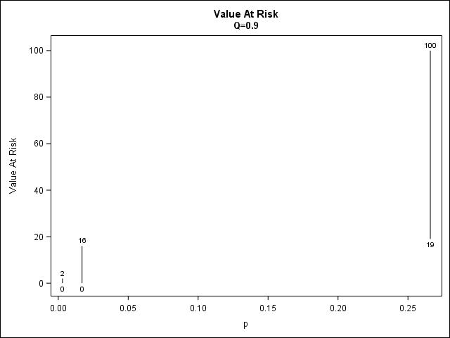
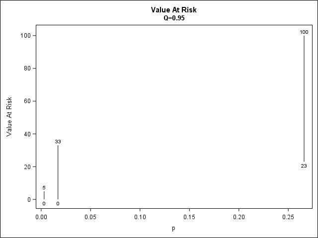
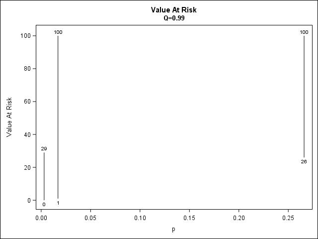
5.1.4 Cross scenario comparisons

The reader can appreciate how model risk increases, when the marginal probability does, and when the risk measure is $\text{VaR}_{\alpha}$, looking at Figure 1. The computation permits to conclude that the VaR range increases with the marginal default probability, and not only with the level of confidence (which is the standard result). Also, both the minimum and the maximum are non decreasing with p.

5.2 Calibration risk

In this Section we examine the behavior of the loss under the three scenarios above for the marginal default probability, when, on top of the marginal, a specific value of the equicorrelation has been selected. We deal with $\mathcal{E(}p,\rho)$ in the three scenarios $p=0.3\%,p=1.7\%$ and $p=26\%$ and provide bounds for $\text{VaR}_{\alpha}$ for three levels of correlation: $\rho=\frac{1}{6};\frac{1}{2};\frac{5}{6}$. Here, the ray densities are analytical as well as their VaR. The bounds are found by computationally searching the maximum and minimum VaR among the ray densities.

As a benchmark we choose an exchangeable Bernoulli mixing model from the credit risk literature. We estimate the $\beta$-mixing model of each scenario and compute its $\text{VaR}_{\alpha}$. Let $S_{\beta}$ be the number of default of the $\beta$-mixing models, we have (for a complete overview see [6]):

$$p_{\beta}(j)=\binom{d}{j}\int_{0}^{1}p^{k}(1-p)^{d-k}d\Psi(p),$$ (5.1)

where $\Psi\sim\beta(a,b)$ the mixing variable. We have

$$\begin{split}&p=E[\Psi]\\ &\mu_{2}=E[\Psi^{2}].\end{split}$$ (5.2)

Therefore we estimate the $\beta$ parameters $a$ and $b$ by

$$\begin{split}&p=\frac{a}{a+b}\\ &\mu_{2}=\frac{a(a+1)}{(a+b)(a+b+1)}.\end{split}$$ (5.3)

Notice that for this model $\rho=0$ is not admissible.

5.2.1 Scenario 1

Table 10 provides the bounds of $\text{VaR}_{\alpha}$ when only correlation is known and it is $\frac{1}{6}$ and the corresponding measures for the $\beta$-mixing model.

Quantile minVaRαsubscriptVaR𝛼\text{VaR}_{\alpha} max VaRαsubscriptVaR𝛼\text{VaR}_{\alpha} β𝛽\beta -VaRαsubscriptVaR𝛼\text{VaR}_{\alpha}
0.9 0 2 0
0.95 0 5 0
0.99 1 22 9
Table 10: $\text{VaR}_{\alpha}$ of the number of defaults for the $\mathcal{E}(0.3\%,\frac{1}{6})$ class of multivariate Bernoulli

Table 11 provides the bounds of $\text{VaR}_{\alpha}$ when only correlation is known and it is $\frac{1}{2}$ and the corresponding $\text{VaR}_{\alpha}$ for the $\beta$-mixing model.

Quantile min VaRαsubscriptVaR𝛼\text{VaR}_{\alpha} max VaRαsubscriptVaR𝛼\text{VaR}_{\alpha} β𝛽\beta -VaRαsubscriptVaR𝛼\text{VaR}_{\alpha}
0.9 0 1 0
0.95 0 3 0
0.99 0 21 4
Table 11: $\text{VaR}_{\alpha}$ of the number of defaults for the $\mathcal{E}(0.3\%,\frac{1}{2})$ class of multivariate Bernoulli

Table 12 provides the bounds of $\text{VaR}_{\alpha}$ when correlation is known and it is $\frac{5}{6}$ and the corresponding measure for the $\beta$-mixing model.

Quantile min VaRαsubscriptVaR𝛼\text{VaR}_{\alpha} max VaRαsubscriptVaR𝛼\text{VaR}_{\alpha} β𝛽\beta -VaRαsubscriptVaR𝛼\text{VaR}_{\alpha}
0.9 0 0 0
0.95 0 1 0
0.99 0 7 0
Table 12: $\text{VaR}_{\alpha}$ of the number of defaults for the $\mathcal{E}(0.3\%,\frac{5}{6})$ class of multivariate Bernoulli

5.2.2 Scenario 2

Table 13 provides the bounds of $\text{VaR}_{\alpha}$ when correlation is known and it is $\frac{1}{6}$ and the the $\beta$-mixing model $\text{VaR}_{\alpha}$.

Quantile min VaRαsubscriptVaR𝛼\text{VaR}_{\alpha} max VaRαsubscriptVaR𝛼\text{VaR}_{\alpha} β𝛽\beta -VaRαsubscriptVaR𝛼\text{VaR}_{\alpha}
0.9 0 16 5
0.95 1 25 11
0.99 2 55 29
Table 13: $\text{VaR}_{\alpha}$ of the number of defaults for the $\mathcal{E}(1.7\%,\frac{1}{6})$ class of multivariate Bernoulli

Table 14 provides the bounds of $\text{VaR}_{\alpha}$ when correlation is known and it is $\frac{1}{2}$ and the corresponding measure for the $\beta$-mixing model.

Quantile minVaRαsubscriptVaR𝛼\text{VaR}_{\alpha} max VaRαsubscriptVaR𝛼\text{VaR}_{\alpha} β𝛽\beta -VaRαsubscriptVaR𝛼\text{VaR}_{\alpha}
0.9 0 9 0
0.95 0 25 5
0.99 1 93 57
Table 14: $\text{VaR}_{\alpha}$ of the number of defaults for the $\mathcal{E}(1.7\%,\frac{1}{2})$ class of multivariate Bernoulli

Table 15 provides the bounds of $\text{VaR}_{\alpha}$ when correlation is known and it is $\frac{5}{6}$ and the corresponding $\text{VaR}_{\alpha}$ for the $\beta$-mixing model.

Quantile min VaRαsubscriptVaR𝛼\text{VaR}_{\alpha} max VaRαsubscriptVaR𝛼\text{VaR}_{\alpha} β𝛽\beta -VaRαsubscriptVaR𝛼\text{VaR}_{\alpha}
0.9 0 3 0
0.95 0 8 0
0.99 61 100 94
Table 15: $\text{VaR}_{\alpha}$ of the number of defaults for the $\mathcal{E}(1.7\%,\frac{5}{6})$ class of multivariate Bernoulli

5.2.3 Scenario 3

Table 16 provides the bounds of $\text{VaR}_{\alpha}$ when correlation is known and it is $\frac{1}{6}$ and the corresponding measures for the $\beta$-mixing model. In this case the number of generators of the class significantly increases. In fact, the class $\mathcal{E}(26.6\%,\frac{1}{6})$ is generated by 32.372 ray densities.

Quantile min VaRαsubscriptVaR𝛼\text{VaR}_{\alpha} max VaRαsubscriptVaR𝛼\text{VaR}_{\alpha} β𝛽\beta -VaRαsubscriptVaR𝛼\text{VaR}_{\alpha}
0.9 21 82 53
0.95 26 100 62
0.99 38 100 76
Table 16: $\text{VaR}_{\alpha}$ of the number of defaults for the $\mathcal{E}(26.6\%,\frac{1}{6})$ class of multivariate Bernoulli

Table 17 provide the bounds of $\text{VaR}_{\alpha}$ when correlation is known and it is $\frac{1}{2}$ and the corresponding measure for the $\beta$-mixing model.

Quantile min $\text{VaR}_{\alpha}$ max $\text{VaR}_{\alpha}$ $\beta$ -$\text{VaR}_{\alpha}$ R
0.9 42 100 82
0.95 56 100 93
0.99 63 100 100
Table 17: $\text{VaR}_{\alpha}$ of the number of defaults for the $\mathcal{E}(26.6\%,\frac{1}{2})$ class of multivariate Bernoulli

Table 18 provide the bounds of $\text{VaR}_{\alpha}$ when correlation is known and it is $\frac{5}{6}$ and the corresponding measure for the $\beta$-mixing model.

Quantile min VaRαsubscriptVaR𝛼\text{VaR}_{\alpha} max VaRαsubscriptVaR𝛼\text{VaR}_{\alpha} β𝛽\beta -VaRαsubscriptVaR𝛼\text{VaR}_{\alpha}
0.9 81 100 100
0.95 86 100 100
0.99 88 100 100
Table 18: $\text{VaR}_{\alpha}$ of the number of defaults for the $\mathcal{E}(26.6\%,\frac{5}{6})$ class of multivariate Bernoulli

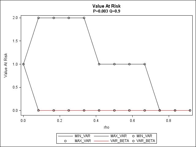
5.2.4 Cross scenario comparisons

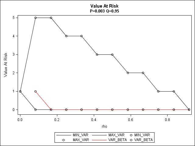
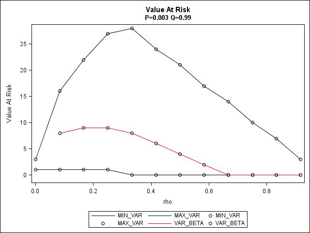
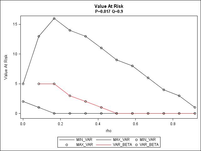
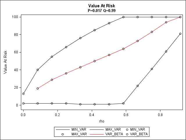
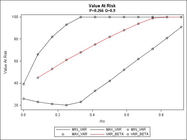
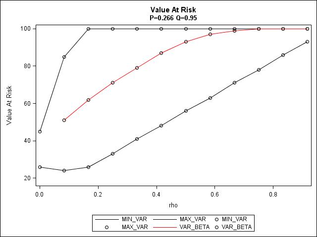
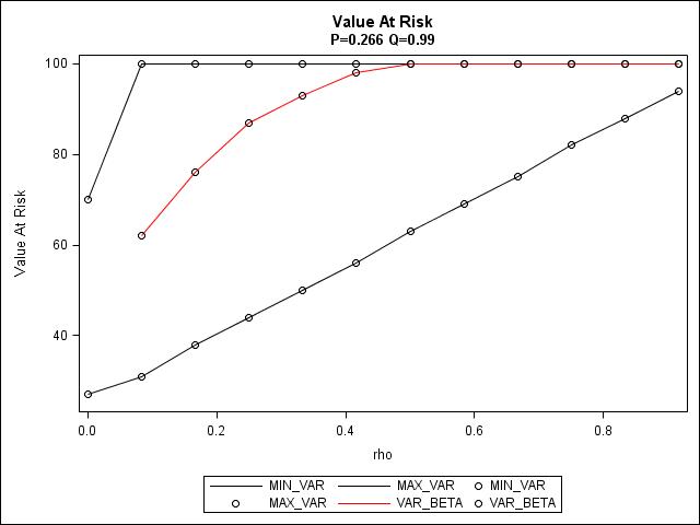
Figures 2, 3 and 4 plot the bounds for VaR when $\rho$ takes equispaced value in the range $[0,\frac{11}{12})$. The reader can appreciate how calibration risk increases, when the marginal probability and the correlation does. It also emerges that the $\text{VaR}_{\alpha}$ of the $\beta$-mixing model sometimes reaches the bound and depending on $p$ and $\rho$ its values with respect to the bounds significantly change. In particular for low $p$ the $\text{VaR}_{\alpha}$ of the $\beta$-mixing model coincides with the minimum $\text{VaR}_{\alpha}$. The plots show that, even if the $\beta$-mixing model is calibrated to match the moments of the Bernoulli, it tends to produce a VaR close to the minimum one for low $p$, and close to the maximum for high $p$. In any case, the width of the band between the minimum and the maximum, together with the specific location of the $\beta$ VaR within it, give a sense of how wrong the risk appreciation can go, when calibrating a specific correlation, and how stringent is the choice of a specific multivariate distribution within that calibration.

6 Conclusions

Measuring model risk in credit and default modeling is important, at least to have a sense of the consequences of mispricing of financial products, forecasting errors etc. Since, at present, model risk in credit and default cannot be avoided, we can try to measure it. This paper does exactly that, in a very general context (exchangeable, equicorrelated Bernoulli), using two popular risk measures, VaR and ES. The main contributions are the closed form results for the VaR bounds and the moments of the multivariate distributions, as well as the numerical examples which show how big model risk can be, with a portfolio of 100 obligors with equal exposure, especially when the marginal default probability is high.

References

  • [1] R. C. Merton, “On the pricing of corporate debt: The risk structure of interest rates,” The Journal of finance, vol. 29, no. 2, pp. 449–470, 1974.
  • [2] R. A. Jarrow and S. M. Turnbull, Credit Risk: Drawing the Analogy, vol. 5. 1992.
  • [3] T. Bielecki, M. Jeanblanc, and M. Rutkowski, “Credit risk modeling.,” CSFI Lecture Notes Series, vol. 2, 2009.
  • [4] U. Cherubini, E. Luciano, and W. Vecchiato, Copula methods in finance. John Wiley & Sons, 2004.
  • [5] D. Duffie and K. Singleton, “Credit risk: Pricing, measurement, and menagement,” 2003.
  • [6] A. J. McNeil, R. Frey, and P. Embrechts, Quantitative risk management, vol. 3. Princeton university press, 2005.
  • [7] P. Embrechts, A. McNeil, and D. Straumann, “Correlation and dependence in risk management: Properties and pitfalls.,” Risk management: value at risk and beyond, ed. Dempster, M.
  • [8] P. Embrechts, A. Höing, and A. Juri, “Using copulae to bound the value-at-risk for functions of dependent risks,” Finance and Stochastics, vol. 7, no. 2, pp. 145–167, 2003.
  • [9] R. Fontana and P. Semeraro, “Representation of multivariate bernoulli distributions with a given set of specified moments,” Journal of Multivariate Analysis, vol. 168, pp. 290–303, 2018.
  • [10] M. Terzer, Large scale methods to enumerate extreme rays and elementary modes. PhD thesis, ETH Zurich, 2009.
  • [11] “Default, transition, and recovery: 2017 annual global corporate default study and rating transitions.”
Figure 1: VAR ranges for $p=0.03\%;1.7\%;26.6\%$
Refer to caption
Refer to caption
Refer to caption
Figure 2: VAR bounds for $p=0.03\%$ and different $\rho$ and $\beta$-mixing model VAR
Refer to caption
Refer to caption
Refer to caption
Figure 3: VAR bounds for $p=1.7\%$ and different $\rho$ and $\beta$-mixing model VAR
Refer to caption
Refer to caption
Refer to caption
Figure 4: VAR bounds for $p=26.6\%$ and different $\rho$ and $\beta$-mixing model VAR
Refer to caption
Refer to caption
Refer to caption