TESTING THE GRAVITATIONAL REDSHIFT WITH GALILEO SATELLITES

P. Delva¹ N. Puchades^2,1 E. Schönemann³ F. Dilssner³ C. Courde⁴ S. Bertone⁵ F. Gonzalez⁶ A. Hees¹ Ch. Le Poncin-Lafitte¹ F. Meynadier¹ R. Prieto-Cerdeira⁶ B. Sohet¹ J. Ventura-Traveset⁷ P. Wolf¹ ¹SYRTE, Observatoire de Paris, Université PSL, CNRS, Sorbonne Université, LNE, 61 avenue de l’Observatoire 75014 Paris France ²Departamento de Astronomia y Astrofisica - Valencia University ³European Space Operations Center, ESA/ESOC, Darmstadt Germany ⁴UMR Geoazur, Université de Nice, Observatoire de la Côte d’Azur, 250 rue A. Einstein, F-06560 Valbonne, France ⁵Astronomical Institute, University of Bern, Sidlerstrasse 5 CH-3012 Bern, Switzerland ⁶European Space and Technology Centre, ESA/ESTEC, Noordwijk, The Netherlands ⁷European Space and Astronomy Center, ESA/ESAC, Villanueva de la Cañada, Spain

Abstract

We present the results of the analysis of the GREAT (Galileo gravitational Redshift test with Eccentric sATellites) experiment from SYRTE (Observatoire de Paris), funded by the European Space Agency. An elliptic orbit induces a periodic modulation of the fractional frequency difference between a ground clock and the satellite clock, while the good stability of Galileo clocks allows to test this periodic modulation to a high level of accuracy. Galileo satellites GSAT0201 and GSAT0202, with their large eccentricity and on-board H-maser clocks, are perfect candidates to perform this test. By analyzing 1008 days of eccentric Galileo satellites data we measure the fractional deviation of the gravitational redshift from the prediction by general relativity to be $(0.19\pm 2.48)\text{\times}{10}^{-5}$ at 1 sigma, improving the best previous test by Gravity Probe A by a factor 5.6. Moreover, we apply the exact same analysis to two almost circular Galileo satellites, in order to show the robustness of the method. By analyzing 899 days of circular Galileo satellites data we measure the fractional deviation of the gravitational redshift from the prediction by general relativity to be $(0.29\pm 2.00)\text{\times}{10}^{-2}$ at 1 sigma.

1 Testing the Einstein equivalence principle with atomic clocks

General Relativity is based on two fundamental hypothesis: the Einstein Equivalence Principle (EEP) and the Einstein field equations. Following Will [1], EEP can be divided into three sub-principles: (i) the Weak Equivalence Principle: if any uncharged test body is placed at an initial event in space-time and given an initial velocity there, then its subsequent trajectory will be independent of its internal structure and composition; (ii) the Local Position Invariance (LPI): the outcome of any local non-gravitational test experiment is independent of where and when in the universe it is performed; (iii) and the Local Lorentz Invariance: the outcome of any local non-gravitational test experiment is independent of the velocity of the (freely falling) apparatus.

Tests of Lorentz Invariance have been performed using comparisons of atomic clocks onboard GPS satellites w.r.t. ground clocks [2], and more recently using an international network of optical clocks compared with optical fibres [3]. Test of Lorentz Invariance can be performed also in the Matter Sector [4, 5, 6, 7]. Test of LPI can be performed by searching for variations in the constants of Nature [8]. Several types of variation can occur depending on the particular theory: linear temporal drift [9, 10, 11, 12, 13]; spatial variation w.r.t. the Sun gravitational potential [9, 14, 11, 15]; harmonic temporal variation [16, 17]; and transients [18, 19, 20, 21]. Harmonic temporal variations and transients usually occurs when standard matter couples anormally to a field which can be linked to light dark matter.

Finally, LPI can be tested with a clock redshift experiment, where the gravitational redshift can be measured. It was observed for the first time in the Pound-Rebka-Snider experiment [22, 23, 24, 25]. In a clock redshift experiment, the fractional frequency difference $z=\Delta\nu/\nu$ between two identical clocks placed at different locations in a static gravitational field is measured. The EEP predicts $z=\Delta U/c^{2}$ for stationary clocks, where $\Delta U$ is the gravitational potential difference between the locations of the receiver and the emitter, and $c$ is the velocity of light in vacuum. A simple and convenient formalism to test the gravitational redshift is to introduce a new parameter $\alpha$ defined through [26]:

z=\frac{\Delta\nu}{\nu}=(1+\alpha)\frac{\Delta U}{c^{2}}

(1)

with $\alpha$ vanishing when the EEP is valid. The most precise test of the gravitational redshift until recently has been realized with the Vessot-Levine rocket experiment in 1976, also named the Gravity Probe A (GP-A) experiment [27, 28, 29]. The frequency differences between a space borne hydrogen maser clock and ground hydrogen masers were measured thanks to a continuous two-way microwave link. The gravitational redshift prediction was verified with $1.4\text{\times}{10}^{-4}$ uncertainty. A recent test with the clocks of Galileo 5 and 6 satellites improved this limit to $2.5\text{\times}{10}^{-5}$ uncertainty [30, 31, 32]. The ACES experiment will test the gravitational redshift to around 2– $3\text{\times}{10}^{-6}$ accuracy [33]. Furthermore, other projects like STE-QUEST propose to test the gravitational redshift at the level of $10^{-7}$ . Finally, observations with the RadioAstron telescope reach today an accuracy [34] of $3\text{\times}{10}^{-2}$ , and may reach [35] an accuracy of the order of $10^{-5}$ in the future.

In this article we report on the recent test of gravitational redshift using eccentric Galileo satellites [30], where the fractional deviation of the gravitational redshift from the prediction by general relativity was reported to be $(0.19\pm 2.48)\text{\times}{10}^{-5}$ , therefore compatible with general relativity. Moreover, we apply the same analysis to two circular Galileo satellites. Even if the accuracy of the test with circular satellites is 3 orders of magnitude smaller than the one with eccentric satellites, it is worth to verify that the exact same analysis lead to a robust estimation of uncertainties, and especially the ones due to systematics. Such a test with circular satellites has been performed with GPS in the TOPEX/POSEIDON Relativity Experiment [36], reaching an accuracy of $2.2\text{\times}{10}^{-2}$ , which is almost the same as our result with circular Galileo satellites.

2 Test of the Gravitational redshift with Galileo eccentric satellites

Galileo is the European Global Navigation Satellite System (GNSS). The space segment consists in 24 operational satellites and 6 spares satellites in medium Earth orbit, placed on three different orbital planes. There are actually 26 launched satellites. When the constellation will be completed, ten satellites will be spread evenly around each orbital plane. A global network of ground sensor stations is receiving signals from the Galileo satellites, and sending that information to control centres located in Europe. The control centres are computing the signals in order to find orbit solutions and synchronise the time signal of the satellites. The control centres are sending this information to the satellites via a global network of 5 up-link stations. Then, the satellites can send the relevant timing and positioning information to the receivers.

Refer to caption — Figure 1: The original (in red) and corrected (in blue) orbits of the fifth and sixth Galileo satellites, along with that of the first four satellites (green) (Copyright ESA)

ESA supports science done with Galileo through the GNSS Science Support Centre (GSSC: gssc.esa.int) and the GNSS Science Advisory Committee (GSAC). Today, more than 100 GNSS satellites have been launched, with a global coverage and continuous measurements. Their scientific use led to major contributions in Earth Science, Fundamental Physics, Metrology and many other fields. Before the second generation of Galileo satellites, an intermediate batch of 6 satellites will be launched between 2024 and 2026. These satellites will embark experimental instruments, which will be the occasion to perform new science with Galileo.

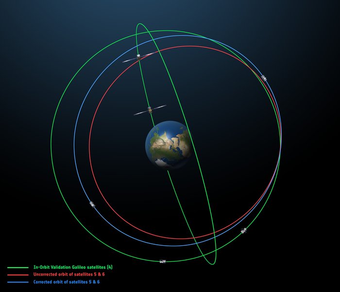
Galileo satellites GSAT0201 and GSAT0202 were launched on a Soyuz rocket on August, 2014 on the wrong orbit due to a technical problem. The anomaly occurred during the flight of Fregat, the launcher’s fourth stage, 35 minutes after liftoff, leading to an anomaly in the orbital injection of the satellites ¹¹1Arianespace Press Release: “Soyuz Flight VS09: Independent Inquiry Board announces definitive conclusions concerning the Fregat upper stage anomaly”, October 08, 2014.. Instead of a nominal circular orbit, the satellites were placed on a very eccentric orbit with 0.21 eccentricity (see Fig.1, red orbit). The orbital error resulted from a temporary interruption of the joint hydrazine propellant supply to the thrusters, caused by freezing of the hydrazine, which resulted from the proximity of hydrazine and cold helium feed lines. This caused a loss of inertial reference and an error in the thrust orientation for the launcher’s fourth stage. Soon after the launch, the European Space Agency searched for a suitable orbit for these satellites such that they could be operational ²²2ESA Press Release: “Galileo satellite recovered and transmitting navigation signals”, December 03, 2014.. A total of 11 manoeuvres were performed to circularize the orbit, such that the satellite’s Earth sensor can be used continuously, keeping its main antenna oriented towards Earth and allowing its navigation payload to be switched on. The final orbit of the two salvaged satellites is still very eccentric, with an eccentricity of 0.16 (see Fig.1, blue orbit).

The Galileo satellites GSAT0201 and GSAT0202, with their high eccentricity, are perfect candidates for a test of the gravitational redshift. Indeed, an elliptic orbit induces a periodic modulation of the clock proper time at orbital frequency. For a Keplerian orbit it can be shown that the relation between proper time $\tau$ of the satellite clock and coordinate time $t$ is:

\tau(t)=\left(1-\frac{3Gm}{2ac^{2}}\right)t-\frac{2\sqrt{Gma}}{c^{2}}e\sin{E(t)}+\text{Cst}

(2)

where $Gm$ is the gravitational parameter of the Earth, $a$ , $e$ and $E$ are the semi-major axis, the eccentricity and the eccentric anomaly of the satellite, respectively, and $c$ is the velocity of light in vacuum.

The first term in Eq.(2), linear in time, results in a constant frequency shift between the satellite clock and a ground clock, which is $\approx$40\text{\,}\mathrm{\SIUnitSymbolMicro s}\text{\,}{\mathrm{d}}^{-1}$$ assuming a nominal 10.23 MHz frequency for the Passive Hydrogen Maser (PHM) onboard the satellite. However, each PHM clock is also affected by an intentional frequency offset ( $\approx$-6\text{\,}\mathrm{\SIUnitSymbolMicro s}\text{\,}{\mathrm{d}}^{-1}$$ ) to this nominal frequency which explains an observed drift of $\approx$34\text{\,}\mathrm{\SIUnitSymbolMicro s}\text{\,}{\mathrm{d}}^{-1}$$ . Additionally, after each activation the PHM clock retraces to the nominal frequency with an accuracy not better than $\pm$0.18\text{\,}\mathrm{\SIUnitSymbolMicro s}\text{\,}{\mathrm{d}}^{-1}$$ . We account for this unknown frequency offset (together with the known $\approx$34\text{\,}\mathrm{\SIUnitSymbolMicro s}\text{\,}{\mathrm{d}}^{-1}$$ ) by removing from the measured clock bias a daily linear fit (DLF).

The second term in Eq.(2) is proportional to the eccentricity of the satellite and periodic with a period equal to the orbital period of the satellite. The amplitude of this term amounts to $\approx$800\text{\,}\mathrm{ns}$$ peak-to-peak. To measure this periodic effect with a good accuracy, one needs a good stability of the clock over the orbital period, around $13\text{\,}\mathrm{h}$ , which is the case of the Galileo clock, designed to be very stable over one day. Moreover, the nominal satellite lifetime is around 15 years, which allows to reduce the statistical uncertainty of the gravitational redshift test, and the satellites are permanently monitored by several ground receivers.

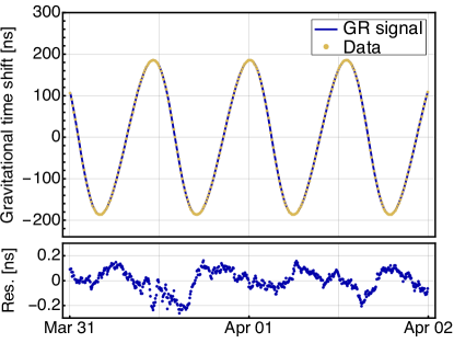
The orbit of the Galileo satellites is not Keplerian. Therefore we cannot use Eq.(2) to calculate the total redshift. Instead, one has to use the full formula from GR, which can be found in [30]. As input to the full proper time to coordinate time transformation, we use an orbit and clock solution generated by ESA’s Navigation Support Office, located at the European Space Operations Centre (ESOC). The proper time to coordinate time transformation equation can be split into different contributions: the periodic gravitational redshift amounts to $400\text{\,}\mathrm{ns}$ peak-to-peak (see Fig.2); the Earth flatness leads to a $40\text{\,}\mathrm{ps}$ peak-to-peak periodic effect at twice the orbital frequency; finally, tidal effects from the Moon and the Sun lead to a periodic signal of around $12\text{\,}\mathrm{ps}$ peak-to-peak, higher than the uncertainty goal of the experiment which is $4\text{\,}\mathrm{ps}$ .

The data analysis is done in three steps. First, we fit a model for the stochastic noise to the corrected clock bias residuals. In a second step, we fit our theoretical model to the corrected clock bias by using a Monte Carlo approach, using the stochastic noise model estimated in the first step. This gives us the fitted value for the LPI violation $\alpha$ as well as an estimation of its statistical uncertainty. In a third step, we estimate the systematic uncertainty by considering the main sources of systematics: effects of magnetic field, of temperature and mismodelling of the orbital motion of the satellites. These three steps are described in details in [30].

Finally, by analysing 1008 days of data from the two eccentric Galileo satellites, GSAT0201 and GSAT0202, and through a careful analysis of systematic effects, we were able to improve the gravitational redshift test done by GP-A in 1976 by a factor 5.6, down to $\alpha=$(0.19\pm 2.48)\text{\times}{10}^{-5}$$ . The different sources of uncertainty are given in Table 1.

3 Test of the Gravitational redshift with Galileo circular satellites

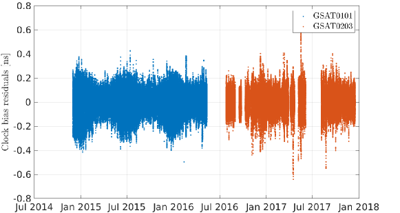
Now we apply exactly the same data analysis to two chosen circular satellites. The master clock on board the Galileo satellites may change over time due to maintenance routine. There are two PHM clocks as well as two rubidium clocks (RAFS) on board each of the satellites. The RAFS is usually ten times noisier than than the PHM. The circular satellites have been chosen such that one of the PHM clock was operational for more than one year. We did not use the RAFS clock. We choose one satellite from the IOV (In-Orbit Validation) generation, GSAT0101, which was launched in October 21, 2011. Moreover, we choose another satellite from the FOC (Full Operational Capability) generation, GSAT0203, which was launched in March 27, 2015. The pre-fit residuals of the clock bias from these two satellites are shown in Fig.3. The data analysis contains 518 days of data from GSAT0101 and 381 days of data from GSAT0203, spanning from November 2014 to December 2017.

The different sources of uncertainty are given in Table 1. When we quadratically add the statistical and systematic uncertainties due to each considered error source, we obtain for the LPI violation parameter $\alpha=$(0.71\pm 1.89)\text{\times}{10}^{-2}$$ for GSAT0101 and $\alpha=$(-5.31\pm 4.86)\text{\times}{10}^{-2}$$ for GSAT0203. Finally, we combine the data from both circular satellites using a global Monte-Carlo least square analysis, by applying a weight inversely proportional to their orbit uncertainty given in Table 1, as we did for the eccentric satellites. We obtain for the LPI violation parameter $\alpha=$(0.29\pm 2.00)\text{\times}{10}^{-2}$$ . The aacuracy of the test is slightly degraded in the combination compared to GSAT0101 alone, because of the high orbit uncertainty of GSAT0203, however the bias is closer to zero in the combined solution.

4 conclusion

To conclude, we reported the use of eccentric Galileo satellites to perform the best test of the gravitational redshift to date [30]. By analysing 1008 days of data from the two eccentric Galileo satellites, GSAT0201 and GSAT0202, and through a careful analysis of systematic effects, we were able to improve the gravitational redshift test done by GP-A in 1976 by a factor 5.6, down to $\alpha=$(0.19\pm 2.48)\text{\times}{10}^{-5}$$ . Our result is at the lower edge of the predicted sensitivity in [31]. Moreover, we applied the same analysis to two circular Galileo satellites, GSAT0101 and GSAT0203, obtaining $\alpha=$(0.29\pm 2.00)\text{\times}{10}^{-2}$$ . This new result shows the robustness of the uncertainty analysis we developed for the eccentric satellites. Finally, the ACES experiment will improve this result by one order of magnitude in 2020. Ground optical clock comparisons might also improve our result in the coming years.

	LPI	Total	Stat.	Orbit	Temperature	Magnetic field
	violation	uncertainty	unc.	unc.	unc.	tot. unc.
Eccentric	[ $\times 10^{-5}$ ]	[ $\times 10^{-5}$ ]	[ $\times 10^{-5}$ ]	[ $\times 10^{-5}$ ]	[ $\times 10^{-5}$ ]	(X/Y/Z) [ $\times 10^{-5}$ ]
GSAT0201	$-0.77$	$2.73$	$1.48$	$1.09$	$0.59$	$1.93$ $(0.52,-0.36,1.82)$
GSAT0202	$6.75$	$5.62$	$1.41$	$5.09$	$0.13$	$1.92$ $(-0.07,0.58,1.83)$
Combined	$0.19$	$2.48$	$1.32$	$0.70$	$0.55$	$1.91$ $(0.48,-0.29,1.82)$
Circular	[ $\times 10^{-2}$ ]	[ $\times 10^{-2}$ ]	[ $\times 10^{-2}$ ]	[ $\times 10^{-2}$ ]	[ $\times 10^{-2}$ ]	(X/Y/Z) [ $\times 10^{-2}$ ]
GSAT0101	$0.71$	$1.89$	$0.57$	$1.39$	$0.07$	$1.15$ $(-0.07,1.15,-0.01)$
GSAT0203	$-5.31$	$4.86$	$0.90$	$4.58$	$0.07$	$1.35$ $(0.05,1.35,0.00)$
Combined	$0.29$	$2.00$	$0.55$	$1.53$	$0.07$	$1.16$ $(-0.06,1.16,-0.01)$

Table 1: Final result of the EEP/LPI test. Each row is a separate output from fits of each satellite data and models, and a combined fit of 2 satellites data and models (either eccentric or circular). The uncertainties due to systematic effects are evaluated independently from the clock data, and are the result of individual fits of models of systematics (for temperature and magnetic field), and a fit of SLR residuals for the orbit uncertainty, thus giving an upper limit of each effect. A single value is computed for the magnetic field uncertainty by summing in quadrature the X/Y/Z values. The total uncertainty column, for each row, is derived from the quadratic sum of the individual uncertainties to the right.

Acknowledgments

We acknowledge financial support from ESA within the GREAT (Galileo gravitational Redshift Experiment with eccentric sATellites) project, from Paris Observatory/GPhys specific action.

References

[1] C. M. Will. Theoretical Frameworks for Testing Relativistic Gravity. II. Parametrized Post-Newtonian Hydrodynamics, and the Nordtvedt Effect. The Astrophysical Journal, 163:611, 1971.
[2] Peter Wolf and Gérard Petit. Satellite test of special relativity using the global positioning system. Phys. Rev. A, 56(6):4405–4409, 1997.
[3] P. Delva and J. Lodewyck. Test of special relativity using a fiber network of optical clocks. In Proceedings of the Rencontres de Moriond, Gravitation, March 25-April 01, 2017, La Thuile, Italy, 2017.
[4] Peter Wolf, Fréderic Chapelet, Sébastien Bize, and André Clairon. Cold Atom Clock Test of Lorentz Invariance in the Matter Sector. Phys. Rev. Lett., 96(6):060801, 2006.
[5] Michael A. Hohensee, Steven Chu, Achim Peters, and Holger Müller. Equivalence Principle and Gravitational Redshift. Phys. Rev. Lett., 106(15):151102, 2011.
[6] H. Pihan-Le Bars, C. Guerlin, R.-D. Lasseri, J.-P. Ebran, Q. G. Bailey, S. Bize, E. Khan, and P. Wolf. Lorentz-symmetry test at Planck-scale suppression with nucleons in a spin-polarized ${̂133}\mathrm{}Cs{}$ cold atom clock. Phys. Rev. D, 95(7):075026, 2017.
[7] Christian Sanner, Nils Huntemann, Richard Lange, Christian Tamm, Ekkehard Peik, Marianna S. Safronova, and Sergey G. Porsev. Optical clock comparison for Lorentz symmetry testing. Nature, 567(7747):204–208, 2019.
[8] Jean-Philippe Uzan. Varying Constants, Gravitation and Cosmology. Living Reviews in Relativity, 14(2), 2011.
[9] J. Guéna, M. Abgrall, D. Rovera, P. Rosenbusch, M. E. Tobar, Ph. Laurent, A. Clairon, and S. Bize. Improved tests of local position invariance using ${}^{87}\mathrm{Rb}$ and ${}^{133}\mathrm{Cs}$ fountains. Phys. Rev. Lett., 109(8):080801, 2012.
[10] T. Rosenband, D. B. Hume, P. O. Schmidt, C. W. Chou, A. Brusch, L. Lorini, W. H. Oskay, R. E. Drullinger, T. M. Fortier, J. E. Stalnaker, S. A. Diddams, W. C. Swann, N. R. Newbury, W. M. Itano, D. J. Wineland, and J. C. Bergquist. Frequency Ratio of Al+ and Hg+ Single-Ion Optical Clocks; Metrology at the 17th Decimal Place. Science, 319(5871):1808–1812, 2008.
[11] N. Leefer, C. T. M. Weber, A. Cingöz, J. R. Torgerson, and D. Budker. New Limits on Variation of the Fine-Structure Constant Using Atomic Dysprosium. Phys. Rev. Lett., 111(6):060801, 2013.
[12] R. M. Godun, P. B. R. Nisbet-Jones, J. M. Jones, S. A. King, L. A. M. Johnson, H. S. Margolis, K. Szymaniec, S. N. Lea, K. Bongs, and P. Gill. Frequency ratio of two optical clock transitions in ${}^{171}{\mathrm{yb}}^{+}$ and constraints on the time variation of fundamental constants. Phys. Rev. Lett., 113(21):210801, 2014.
[13] N. Huntemann, B. Lipphardt, Chr. Tamm, V. Gerginov, S. Weyers, and E. Peik. Improved limit on a temporal variation of ${m}_{p}/{m}_{e}$ from comparisons of ${\mathrm{yb}}^{+}$ and cs atomic clocks. Phys. Rev. Lett., 113(21):210802, 2014.
[14] Steven Peil, Scott Crane, James L. Hanssen, Thomas B. Swanson, and Christopher R. Ekstrom. Tests of local position invariance using continuously running atomic clocks. Phys. Rev. A, 87(1):010102, 2013.
[15] N. Ashby, T. P. Heavner, S. R. Jefferts, T. E. Parker, A. G. Radnaev, and Y. O. Dudin. Testing Local Position Invariance with Four Cesium-Fountain Primary Frequency Standards and Four NIST Hydrogen Masers. Phys. Rev. Lett., 98(7):070802, 2007.
[16] Ken Van Tilburg, Nathan Leefer, Lykourgos Bougas, and Dmitry Budker. Search for Ultralight Scalar Dark Matter with Atomic Spectroscopy. Phys. Rev. Lett., 115(1):011802, 2015.
[17] A. Hees, J. Guéna, M. Abgrall, S. Bize, and P. Wolf. Searching for an Oscillating Massive Scalar Field as a Dark Matter Candidate Using Atomic Hyperfine Frequency Comparisons. Phys. Rev. Lett., 117(6):061301, 2016.
[18] A. Derevianko and M. Pospelov. Hunting for topological dark matter with atomic clocks. Nat Phys, 10(12):933–936, 2014.
[19] P. Wcisło, P. Morzyński, M. Bober, A. Cygan, D. Lisak, R. Ciuryło, and M. Zawada. Experimental constraint on dark matter detection with optical atomic clocks. Nature Astronomy, 1:0009, 2016.
[20] Benjamin M. Roberts, Geoffrey Blewitt, Conner Dailey, Mac Murphy, Maxim Pospelov, Alex Rollings, Jeff Sherman, Wyatt Williams, and Andrei Derevianko. Search for domain wall dark matter with atomic clocks on board global positioning system satellites. Nature Communications, 8(1):1195, 2017.
[21] P. Wcisło, P. Ablewski, K. Beloy, S. Bilicki, M. Bober, R. Brown, R. Fasano, R. Ciuryło, H. Hachisu, T. Ido, J. Lodewyck, A. Ludlow, W. McGrew, P. Morzyński, D. Nicolodi, M. Schioppo, M. Sekido, R. Le Targat, P. Wolf, X. Zhang, B. Zjawin, and M. Zawada. New bounds on dark matter coupling from a global network of optical atomic clocks. Science Advances, 4(12):eaau4869, 2018.
[22] R. V. Pound and G. A. Rebka. Apparent Weight of Photons. Phys. Rev. Lett., 4(7):337–341, 1960.
[23] R. V. Pound and G. A. Rebka. Gravitational Red-Shift in Nuclear Resonance. Phys. Rev. Lett., 3(9):439–441, 1959.
[24] R. V. Pound and G. A. Rebka. Resonant absorption of the 14.4-kev $\gamma$ ray from 0.10- $\mu$ sec ${\mathrm{fe}}^{57}$ . Phys. Rev. Lett., 3(12):554–556, 1959.
[25] R. V. Pound and J. L. Snider. Effect of Gravity on Gamma Radiation. Phys. Rev., 140(3B):B788–B803, 1965.
[26] C. M. Will. The Confrontation between General Relativity and Experiment. Living Reviews in Relativity, 17:4, 2014.
[27] R. F. C. Vessot, M. W. Levine, E. M. Mattison, E. L. Blomberg, T. E. Hoffman, G. U. Nystrom, B. F. Farrel, R. Decher, P. B. Eby, C. R. Baugher, J. W. Watts, D. L. Teuber, and F. D. Wills. Test of Relativistic Gravitation with a Space-Borne Hydrogen Maser. Phys. Rev. Lett., 45(26):2081–2084, 1980.
[28] R. F. C. Vessot and M. W. Levine. A test of the equivalence principle using a space-borne clock. Gen Relat Gravit, 10(3):181–204, 1979.
[29] Robert F. C. Vessot. Clocks and spaceborne tests of relativistic gravitation. Advances in Space Research, 9(9):21–28, 1989.
[30] P. Delva, N. Puchades, E. Schönemann, F. Dilssner, C. Courde, S. Bertone, F. Gonzalez, A. Hees, Ch. Le Poncin-Lafitte, F. Meynadier, R. Prieto-Cerdeira, B. Sohet, J. Ventura-Traveset, and P. Wolf. Gravitational Redshift Test Using Eccentric Galileo Satellites. Phys. Rev. Lett., 121(23):231101, 2018.
[31] P. Delva, A. Hees, S. Bertone, E. Richard, and P. Wolf. Test of the gravitational redshift with stable clocks in eccentric orbits: Application to Galileo satellites 5 and 6. Class. Quantum Grav., 32(23):232003, 2015.
[32] Sven Herrmann, Felix Finke, Martin Lülf, Olga Kichakova, Dirk Puetzfeld, Daniela Knickmann, Meike List, Benny Rievers, Gabriele Giorgi, Christoph Günther, Hansjörg Dittus, Roberto Prieto-Cerdeira, Florian Dilssner, Francisco Gonzalez, Erik Schönemann, Javier Ventura-Traveset, and Claus Lämmerzahl. Test of the Gravitational Redshift with Galileo Satellites in an Eccentric Orbit. Phys. Rev. Lett., 121(23):231102, 2018.
[33] F. Meynadier, P. Delva, C. le Poncin-Lafitte, C. Guerlin, and P. Wolf. Atomic clock ensemble in space (ACES) data analysis. Class. Quantum Grav., 35(3):035018, 2018.
[34] N. V. Nunes, N. Bartel, M. F. Bietenholz, M. V. Zakhvatkin, D. A. Litvinov, V. N. Rudenko, L. I. Gurvits, G. Granato, and D. Dirkx. The gravitational redshift monitored with RadioAstron from near Earth up to 350,000 km. Advances in Space Research, 2019.
[35] D. A. Litvinov, V. N. Rudenko, A. V. Alakoz, U. Bach, N. Bartel, A. V. Belonenko, K. G. Belousov, M. Bietenholz, A. V. Biriukov, R. Carman, G. Cimó, C. Courde, D. Dirkx, D. A. Duev, A. I. Filetkin, G. Granato, L. I. Gurvits, A. V. Gusev, R. Haas, G. Herold, A. Kahlon, B. Z. Kanevsky, V. L. Kauts, G. D. Kopelyansky, A. V. Kovalenko, G. Kronschnabl, V. V. Kulagin, A. M. Kutkin, M. Lindqvist, J. E. J. Lovell, H. Mariey, J. McCallum, G. Molera Calvés, C. Moore, K. Moore, A. Neidhardt, C. Plötz, S. V. Pogrebenko, A. Pollard, N. K. Porayko, J. Quick, A. I. Smirnov, K. V. Sokolovsky, V. A. Stepanyants, J. M. Torre, P. de Vicente, J. Yang, and M. V. Zakhvatkin. Probing the gravitational redshift with an Earth-orbiting satellite. Physics Letters A, 2017.
[36] N. Ashby. Relativity in the Global Positioning System. Living Reviews in Relativity, 6:1, 2003.