Soft Subdivision Motion Planning for Complex Planar Robots

Abstract

The design and implementation of theoretically-sound robot motion planning algorithms is challenging. Within the framework of resolution-exact algorithms, it is possible to exploit soft predicates for collision detection. The design of soft predicates is a balancing act between easily implementable predicates and their accuracy/effectivity.

In this paper, we focus on the class of planar polygonal rigid robots with arbitrarily complex geometry. We exploit the remarkable decomposability property of soft collision-detection predicates of such robots. We introduce a general technique to produce such a decomposition. If the robot is an $m$-gon, the complexity of this approach scales linearly in $m$. This contrasts with the $O(m^{3})$ complexity known for exact planners. It follows that we can now routinely produce soft predicates for any rigid polygonal robot. This results in resolution-exact planners for such robots within the general Soft Subdivision Search (SSS) framework. This is a significant advancement in the theory of sound and complete planners for planar robots.

We implemented such decomposed predicates in our open-source Core Library. The experiments show that our algorithms are effective, perform in real time on non-trivial environments, and can outperform many sampling-based methods.

1 Introduction

Motion planning is widely studied in robotics [9, 10, 5]. Many planners are heuristic, i.e., without a priori guarantees of their performance (see below for what we mean by guarantees). In this paper, we are interested in non-heuristic algorithms for the basic planning problem: this basic problem considers only kinematics and the existence of paths. The robot $R_{0}$ is fixed, and the input is a triple $(\alpha,\beta,\Omega)$ where $\alpha,\beta$ are the start and goal configurations of $R_{0}$, and $\Omega\subseteq{\mathbb{R}}^{d}$ is a polyhedral environment in $d=2$ or $3$. The algorithm outputs an $\Omega$-avoiding path from $\alpha$ to $\beta$ if one exists, and NO-PATH otherwise. See Figure 2 for some rigid robots, and also Figure 2 for our GUI interface for path planning.

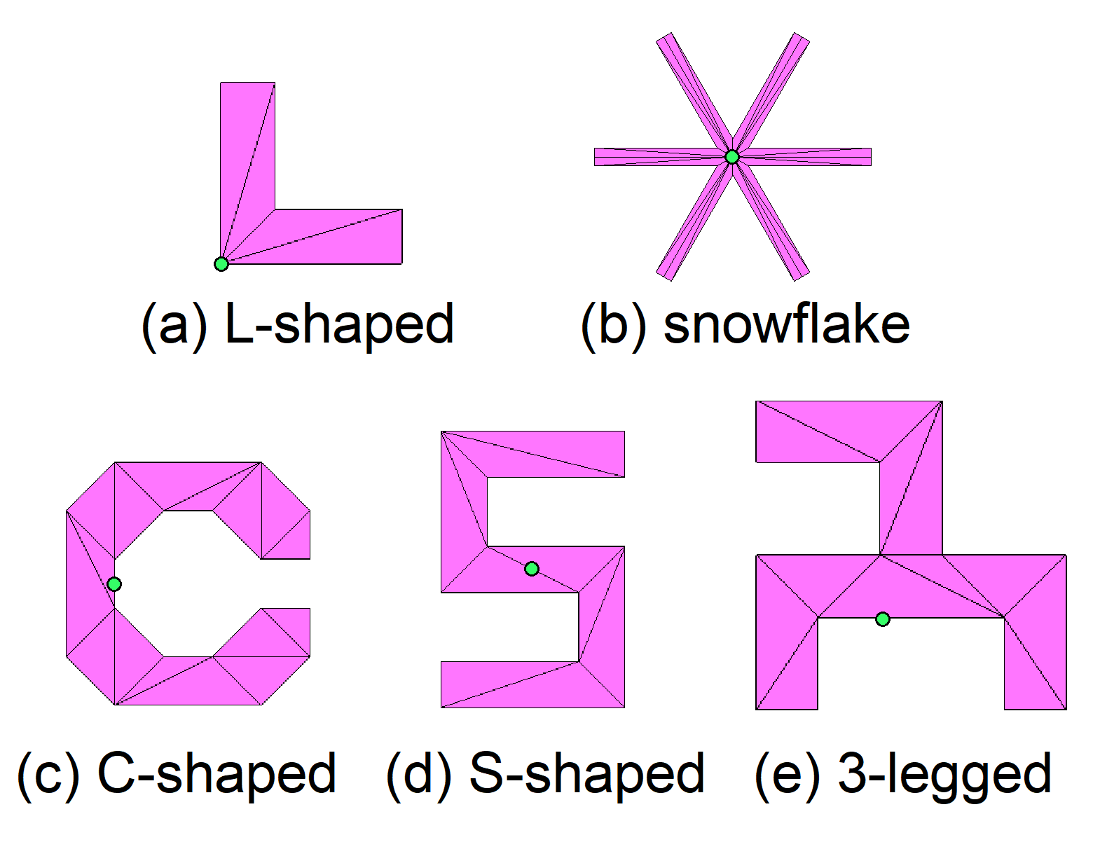
Figure 1: Some rigid planar robots ((a)-(b): star-shaped; (c)-(e): general shaped).

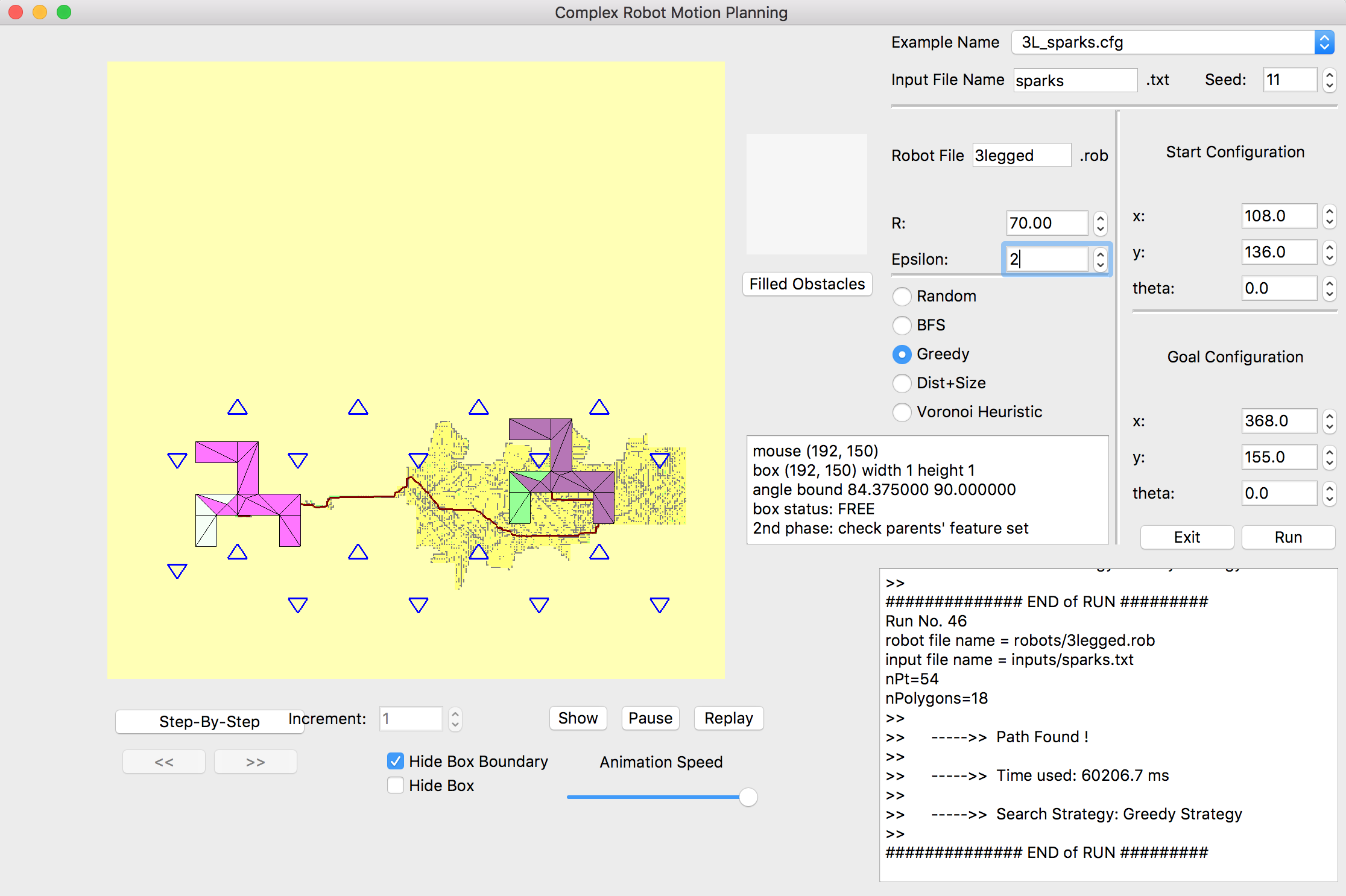
Figure 2: GUI interface for planner for a 3-legged robot.

The basic planning problem ignores issues such as the optimality of paths, robot dynamics, planning in the time dimension, non-holonomic constraints, and other considerations of a real scenario. Despite such an idealization, the solution to this basic planning problem is often useful as the basis for finding solutions that do take into account the omitted considerations. E.g., given a kinematic path, we can plan a smooth trajectory with a homotopic trace.

The algorithms for this basic problem are called “planners.” In theory, it is possible to design exact planners because the basic path planning is a semi-algebraic (non-transcendental) problem. Even when such algorithms are available, exact planners have relatively high complexity and are non-adaptive, even in the plane (see [12]). So we tend to see inexact implementations of exact algorithms, with unclear guarantees. When fully explicit algorithms are known, exact implementation of exact planners is possible using suitable software tools such as the CGAL library [7].

In current robotics [10, 5], those algorithms that are considered practical and have some guarantees may be classified as either resolution-based or sampling-based. The guarantees for the former is the notion of resolution completeness and for the latter, sampling completeness. Roughly speaking, if there exists a path then:
– resolution completeness says that a path will be found if the resolution is fine enough;
– sampling completeness says that a path will be found with high probability if “enough” random samples are taken.
But notice that if there is no path, these criteria are silent; indeed, such algorithms would not halt except by artificial cut-offs. Thus a major effort in the last 20 years of sampling research has been devoted to the so-called “Narrow Passage” problem. It is possible to view this problem as a manifestation of the Halting Problem for the sampling approaches: how can the algorithm halt when there is no path? (A possible approach to address this problem might be to combine sampling with exact computation, as in [13].)

Motivated by such issues, as well as trying to avoid the need for exact computation, we in [15, 16] introduced the following replacement for resolution complete planners: a resolution-exact planner takes an extra input parameter $\epsilon>0$ in addition to $(\alpha,\beta,\Omega)$, and it always halts and outputs either an $\Omega$-avoiding path from $\alpha$ to $\beta$ or NO-PATH. The output satisfies this condition: there is a constant $K>1$ depending on the planner, but independent of the inputs, such that:
– if there is a path of clearance $K\epsilon$, it must output a path;
– if there is no path of clearance $\epsilon/K$, it must output NO-PATH.
Notice that if the optimal clearance lies between $K\epsilon$ and $\epsilon/K$, then the algorithm may output either a path or NO-PATH. So there is output indeterminacy. Note that the traditional way of using $\epsilon$ is to fix $K=1$, killing off indeterminacy. Unfortunately, this also leads us right back to exact computation which we had wanted to avoid. We believe that indeterminacy is a small price to pay in exchange for avoiding exact computation [15]. The practical efficiency of resolution-exact algorithms is demonstrated by implementations of planar robots with 2, 3 and 4 degrees of freedom (DOF) [15, 11, 18], and also 5-DOF spatial robots [8]. All these robots perform in real-time in non-trivial environments. In view of the much stronger guarantees of performance, resolution-exact algorithms might reasonably be expected to have a lower efficiency compared to sampling algorithms. Surprisingly, no such trade-offs were observed: resolution-exact algorithms consistently outperform sampling algorithms. Our 2-link robot [11, 18] was further generalized to have thickness (a feat that exact methods cannot easily duplicate), and can satisfy a non-self-crossing constraint, all without any appreciable slowdown. Finally, these planners are more general than the basic problem: they all work for parametrized families $R_{0}(t_{1},t_{2}\ldots)$ of robots, where $t_{i}$’s are robot parameters. All these suggest the great promise of our approach.

What is New in This Paper. In theoretical path planning, the algorithms often considered simple robots like discs or line segments. In this paper, we consider robots of complex shape, which are more realistic models for real-world robots. We call them “complex robots” (where the complexity comes from the robot geometry rather than from the degrees of freedom). We focus on planar robots that are rigid and connected. Such a robot can be represented by a compact connected polygonal set $R_{0}\subseteq{\mathbb{R}}^{2}$ whose boundary is an $m$-sided polygon, i.e., an $m$-gon. Informally, we call $R_{0}$ a “complex robot” if it is a non-convex $m$-gon for “moderately large” values of $m$, say $m\geq 5$. By this criterion, all the robots in Figure 2 are “complex.” According to [19], no exact algorithms for $m>3$ have been implemented; in this paper, we have robots with $m=18$. To see why complex robots may be challenging, recall that the free space of such robots may have complexity $O((mn)^{3}\log(mn))$ (see [1]) when the robot and environment have complexity $m$ and $n$, respectively. Even with $m$ fixed, this can render the algorithm impractical. For instance, if $m=10$, the algorithm may slow down by 3 orders of magnitude. But our subdivision approach does not have to compute the entire free space before planning a path; hence the worst-case cubic complexity of the free space is not necessarily an issue.

More importantly, we show that the complexity of our new method grows only linearly with $m$. To achieve this, we exploit a remarkable property of soft predicates called “decomposability.” We show how an arbitrary complex robot can be decomposed (via triangulation that may introduce new vertices) into an ensemble of “nice triangles” for which soft predicates are easy to implement. As we see below, there is a significant difference between a single triangle and an ensemble of triangles. In consequence of our new techniques, we can now routinely construct resolution-exact planners for any reasonably complex robot provided by a user. This could lead to a flowering of experimentation algorithmics in this subfield.

Technically, it is important to note that the previous soft predicate construction for a triangle robot in [15, 17] requires that the rotation center, i.e., the origin of the (rotational) coordinate system, be chosen to be the circumcenter of the triangle. But for our new soft predicates the triangles in the triangulation of the complex robot cannot be treated in the same way. This is because all the triangles of the triangulation must share a common origin, to serve as the rotation center of the robot. To ensure easy-to-compute predicates, we introduce the notion of a “nice triangulation” relative to a chosen origin: all triangles must be “nice” relative to this origin. These ideas apply for arbitrary complex robots, but we also exploit the special case of star-shaped robots to achieve stronger results.

Figure 2 shows our experimental setup for complex robots. A demo showing the real-time performance of our algorithms is found in the video clip available through this web link: %YJC???␣To␣be␣Updated!!␣---␣Done!%\url{http://cs.nyu.edu/exact/core\_pages/gallery.html.}%Youtube:%\myHrefxx{https://www.dropbox.com/s/rf0kdw6mxbs255l/complex-robot-demo.mp4?dl=0}.%Exact␣Gallery:https://cs.nyu.edu/exact/gallery/complex/complex-robot-demo.mp4.

Remark. Although it is not our immediate concern to address noisy environments and uncertainties, it is clear that our work can be leveraged to address these issues. E.g., users can choose $\epsilon>0$ to be correlated with the uncertainty in the environment and the precision of the robot sensors. By using weighted Voronoi diagrams [4], we can achieve practical planners that have obstacle-dependent clearances (larger clearance for “dangerous” obstacles).

Previous Related Work. An early work is Zhu-Latombe [21] who also classify boxes into $\mathtt{FREE}$ or $\mathtt{MIXED}$ or $\mathtt{STUCK}$ (using our terminology below). They introduced the concept of M-channels (comprised of $\mathtt{FREE}$ or $\mathtt{MIXED}$ leaf boxes), as a heuristic basis to find an F-channel comprising only of $\mathtt{FREE}$ boxes. Subsequent researchers (Barbehenn-Hutchinson [2] and Zhang-Manocha-Kim [19]) continued this approach. Researchers in resolution-based approaches were interested in detecting the non-existence of paths, but their solutions remain partial because they do not guarantee to always detect non-existence of paths (of sufficient clearances) [3, 19]. The challenge of complex robots was taken up by Manocha’s group who implemented a series of such examples [19]: a “five-gear” robot, a “2-D puzzle” robot a certain “star” robot with 4 DOFs, and a “serial link” robot with 4 DOFs. Except for the “star,” the rest are planar robots.

Overview of the Paper. Section 2 reviews the fundamentals of our soft subdivision approach. Sections 3 and 4 describe our new techniques for star-shaped robots and for general complex robots, respectively. We present the experimental results in Section 5, and conclude in Section 6. All proofs are put in the appendix at the end of the paper. The conference version of this paper appeared in [20].

2 Review: Fundamentals of Soft Subdivision Approach

Our soft subdivision approach includes the following three fundamental concepts (see [15] and the Appendix of [11] for the details):

• Resolution-exactness. This is an alternative replacement for the standard concept of “resolution completeness” in the subdivision literature. Briefly, a planner is resolution-exact if there is a constant $K>1$ such that if there is a path of clearance $K\epsilon$, it will return a path, and if there is no path of clearance $\epsilon/K$, it will return NO-PATH. Here, $\epsilon>0$ is an additional input to the planner, in addition to the normal parameters.

• Soft Predicates. Let ${\,\,\framebox(4.0,7.0)[]{}\,}{\mathbb{R}}^{d}$ be the set of closed axes-aligned boxes in ${\mathbb{R}}^{d}$. We are interested in predicates that classify boxes. Let $C:{\mathbb{R}}^{d}\to\left\{+1,0,-1\right\}$ be an (exact) predicate where $+1,-1$ are called definite values, and $0$ the indefinite value. For motion planning, we may also identify $+1/-1/0$ with $\mathtt{FREE}$/$\mathtt{STUCK}$/$\mathtt{MIXED}$, respectively. In our application, if $p$ is a free configuration, then $C(p)=\mathtt{FREE}$; if $p$ is on the boundary of the free space, $C(p)=\mathtt{MIXED}$; otherwise $C(p)=\mathtt{STUCK}$. We extend $C$ to boxes $B\in{\,\,\framebox(4.0,7.0)[]{}\,}{\mathbb{R}}^{d}$ as follows: for a definite value $v\in\left\{+1,-1\right\}$, $C(B){\color[rgb]{1,0,0}\mathrel{\,:=\,}}v$ if $C(x)=v$ for every $x\in B$. Otherwise, $C(B){\color[rgb]{1,0,0}\mathrel{\,:=\,}}0$. Call $\widetilde{C}:{\,\,\framebox(4.0,7.0)[]{}\,}{\mathbb{R}}^{d}\to\left\{+1,0,-1\right\}$ a “soft version” of $C$ if whenever $\widetilde{C}(B)$ is a definite value, $\widetilde{C}(B)=C(B)$, and moreover, if for any sequence of boxes $B_{i}$ ($i\geq 1$) that converges monotonically to a point $p$, $\widetilde{C}(B_{i})=C(p)$ for $i$ large enough.

• Soft Subdivision Search (SSS) Framework. This is a general framework for a broad class of motion planning algorithms. One must supply a small number of subroutines with fairly general properties in order to derive a specific algorithm. For SSS, we need a predicate to classify boxes in the configuration space as $\mathtt{FREE}$/$\mathtt{STUCK}$/$\mathtt{MIXED}$, a method to split boxes, a method to test if two $\mathtt{FREE}$ boxes are connected by a path of $\mathtt{FREE}$ boxes, and a method to pick $\mathtt{MIXED}$ boxes for splitting. The power of such frameworks is that we can explore a great variety of techniques and strategies. Indeed we introduced the SSS framework to emulate such properties found in the sampling framework.

Feature-Based Approach. Following our previous work  [15, 11], our computation and predicates are ”feature based” whereby the evaluations of box primitives are based on a set $\widetilde{\phi}(B)$ of features associated with the box $B$. Given a polygonal set $\Omega\subseteq{\mathbb{R}}^{2}$ of obstacles, the boundary $\partial\Omega$ may be subdivided into a unique set of corners (points) and edges (open line segments), called the features of $\Omega$. Let $\Phi(\Omega)$ denote this feature set. Our representation of $f\in\Phi(\Omega)$ ensures this local property of $f$: for any point $q$, if $f$ is the closest feature to $q$, then we can decide if $q$ is inside $\Omega$ or not. To see this, first note that if $f$ is a corner, then $q$ is outside $\Omega$ iff $f$ is a convex corner of $\Omega$. But if $f$ is an edge, our representation assigns an orientation to $f$ such that $q$ is inside $\Omega$ iff $q$ lies to the left of the oriented line through $f$.

3 Star-Shaped Robots

We first consider star-shaped robots. A star-shaped region $R$ is one for which there exists a point $A\in R$ such that any line through $A$ intersects $R$ in a single line segment. We call $A$ a center of $R$. Note that $A$ is not unique. When a robot $R_{0}$ is a star-shaped polygon, we decompose $R_{0}$ into a set of triangles that share a common vertex at a center $A$. The rotations of the robot $R_{0}$ about the point $A$ can then be reduced to the rotations of “nice” triangles about $A$. The soft predicates of nice triangles will be easy to implement because their footprints have special representations.

3.1 Nice Shapes for Rotation

Figure 3: Truncated triangular set and swept areas.

From now on, by a triangular set we mean a subset $T\subseteq{\mathbb{R}}^{2}$ which is written as the non-redundant intersection of three closed half-spaces: $T=H_{1}\cap H_{2}\cap H_{3}$. Non-redundant means that we cannot express $T$ as the intersection of only two half-spaces. Note that if $T$ is bounded, this is our familiar notion of a triangle with 3 vertices. But $T$ might be unbounded and have only 2 vertices as in Figure 3(a). If $T$ is a triangular set, we may arbitrarily call one of its vertices the apex and call the resulting $T$ a pointed triangular set. By a truncated triangular set (TTS), we mean the intersection of a pointed triangular set $T$ with any disc centered at its apex $A$, as shown in Figure 3(b).

Notation for Angular Range: It is usual to identify $S^{1}$ (unit circle) with the interval $[0,2\pi]$ where $0$ and $2\pi$ are identified. Let $\alpha\neq\beta\in S^{1}$. Then $[\alpha,\beta]$ denote the range of angles from $\alpha$ counter-clockwise to $\beta$. Thus $[\alpha,\beta]$ and $[\beta,\alpha]$ are complementary ranges in $S^{1}$. If $\Theta=[\alpha,\beta]$, then its width, $|\Theta|$ is defined as $\beta-\alpha$ if $\beta>\alpha$, and $2\pi+\beta-\alpha$ otherwise. Moreover, we will write “$\alpha<\theta<\beta$” to mean that $\theta\in[\alpha,\beta]$.

Fix an arbitrary bounded triangular set $T_{0}$, represented by its three vertices $A,B,C$ where $A$ is the apex. For $\theta\in S^{1}$, let $T_{0}[\theta]$ denote the footprint of $T_{0}$ after rotating $T_{0}$ counter-clockwise (CCW) by $\theta$ about the apex. If $\Theta\subseteq S^{1}$, we write $T_{0}[\Theta]=\bigcup\left\{T_{0}[\theta]:\theta\in\Theta\right\}$. The sets $T_{0}[\theta]$ and $T_{0}[\Theta]$ are called footprints of $T_{0}$ at $\theta$ and $\Theta$, respectively. If $\Theta=[\alpha,\beta]$, write $T_{0}[\alpha,\beta]$ for $T_{0}[\Theta]$, and call $T_{0}[\alpha,\beta]$ the swept area as $T_{0}$ rotates from $\alpha$ to $\beta$.

One of our concerns is to ensure that the swept area $T_{0}[\Theta]$ is “nice.” Consider an example where $[A,B,C]$ is a triangular set with apex $A$ (see Figure 3(c)). Consider the area swept by rotating $[A,B,C]$ in a CCW direction about its apex to position $[A,B^{\prime},C^{\prime}]$. This sweeps out the truncated triangular set shown in Figure 3(b). This truncated triangular set (TTS) is desirable since it can be easily specified by the intersection of three half-spaces and a disc. On the other hand, if $[A,B,C]$ is the triangular set in Figure 3(d), then no rotation of $[A,B,C]$ would sweep out a truncated triangular set. So the triangular set in Figure 3(d) is “not nice,” unlike the triangular set in Figure 3(c).

In general, let $T=[A,B,C]$ be a bounded triangular set. Let $a,b,c$ denote the corresponding angles at $A,B,C$. We say $T$ is nice if either $b$ or $c$ is at least $\pi/2$ ($=90^{\circ}$). We call the corresponding vertex ($B$ or $C$) a nice vertex. Assuming $T$ is non-degenerate and nice, there is a unique nice vertex. In the following, we assume (w.l.o.g.) that $B$ is the nice vertex. The reason for defining niceness is the following.

Lemma 1

Let $T$ be a pointed triangular set. Then $T$ is nice iff for all $\alpha\in S^{1}$ ($0<\alpha<\pi-a$), the footprints $T[0,\alpha]$ and $T[-\alpha,0]$ are truncated triangular sets (TTS).

Lemma 2

Let $R_{0}$ be a star-shaped polygonal region with $A$ as center. If the boundary of $R_{0}$ is an $n$-gon, then we can decompose $R_{0}$ into an essentially disjoint union of at most $2n$ bounded triangular sets (i.e., at most $2n$ triangles) that are nice and have $A$ as the apex.

3.2 Complex Predicates and T/R Subdivision Scheme

For complex robots in general (not necessarily star-shaped), we can exploit the remarkable decomposability property of soft predicates. More specifically, suppose $R_{0}=\cup_{j=1}^{m}T_{j}$ where each $T_{j}$ is a triangle or other shapes and not necessarily pairwise disjoint. If we have soft predicates $\widetilde{C}_{j}(B)$ for each $T_{j}$ (where $B$ is a box), then we immediately obtain a soft predicate for $R_{0}$ defined as follows:

$$\widetilde{C}(B)=\left\{\begin{array}[]{lllllllllllllllllllllllll}\mathtt{FREE}&\textrm{ if each $\widetilde{C}_{j}(B)$ is $\mathtt{FREE}$}\\ \mathtt{STUCK}&\textrm{ if some $\widetilde{C}_{j}(B)$ is $\mathtt{STUCK}$}\\ \mathtt{MIXED}&\textrm{ otherwise.}\end{array}\right.$$ (1)

Let $\sigma>1$ and $\widetilde{C}$ be the soft version of an exact predicate $C$. Recall [15, 17] that $\widetilde{C}$ is $\sigma$-effective if for all boxes $B$, if $C(B)=\mathtt{FREE}$ then $\widetilde{C}(B/\sigma)=\mathtt{FREE}$.

Proposition A.  
(1) $\widetilde{C}$ is a soft version of the exact classification predicate for $R_{0}$.  
(2) Moreover, if each $\widetilde{C}_{j}$ is $\sigma$-effective, then $\widetilde{C}$ is $\sigma$-effective.

We need $\sigma$-effectivity in soft predicates in order to ensure resolution-exactness; see [15, 17] where this proposition was proved. There are two important remarks. First, this proposition is false if the $\widetilde{C}_{j}$ and $\widetilde{C}$ were exact predicates. More precisely, suppose $C$ is the exact predicate for $R_{0}$ and $C_{j}$ is the exact predicate for each $T_{j}$. It is true that if $C(B)=\mathtt{FREE}$ then $C_{j}(B)=\mathtt{FREE}$ for all $j$. But if $C(B)=\mathtt{STUCK}$, it does not follow that $C_{j}(B)=\mathtt{STUCK}$ for some $j$. Second, the predicates $\widetilde{C}_{j}(B)$ for all the $T_{j}$’s must be based on a common coordinate system. As mentioned in Sec. 1, the soft predicate construction for a triangle robot in [15] does not work here. A technical contribution of this paper is the design of soft predicates $\widetilde{C}_{j}(B)$ for all the $T_{j}$’s that are based on a common coordinate system. In the case of star-shaped robots, we apply Lemma 2 and use the apex $A$ as the origin of this common coordinate system. Let $r_{j}$ be the length of the longer edge out of $A$ in $T_{j}$. We define $r_{0}$ as $r_{0}=\max_{j}r_{j}$ (i.e., $r_{0}$ is the radius of the circumcircle of $R_{0}$ centered at $A$).

T/R Splitting. The simplest splitting strategy is to split a box $B\subseteq{\mathbb{R}}^{d}$ into $2^{d}$ congruent subboxes. In the worst case, to reduce all boxes to size $<\epsilon$ requires time $\Omega(\log(1/\epsilon)^{d})$; this complexity would not be practical for $d>3$. In [11, 18] we introduced an effective solution called T/R splitting which can be adapted to configuration space $SE(2)$ in the current paper. Write a box $B\subseteq SE(2)$ as a pair $(B^{t},B^{r})$ where $B^{t}\subseteq{\mathbb{R}}^{2}$ is the translational box and $B^{r}\subseteq S^{1}$ an angular range $\Theta$. We say box $B=(B^{t},B^{r})$ is $\varepsilon$-small if $B^{t}$ and $B^{r}$ are both $\varepsilon$-small; the former means the width of $B^{t}$ is $\leq\varepsilon$; the latter means the angle (in radians) satisfies $|B^{r}|\leq\varepsilon/r_{0}$. Our splitting strategy is to only split $B^{t}$ (leaving $B^{r}=S^{1}$) as long as $B^{t}$ is not $\varepsilon$-small. This is called a T-split, and produces 4 children. Once $B^{t}$ is $\varepsilon$-small, we do binary splits of $B^{r}$ (called R-split) until $B^{r}$ is $\varepsilon$-small. We discard $B$ when it is $\varepsilon$-small. The following lemma (and proof) in [15] can be carried over here:

Lemma 3

([15]) Assume $0<\varepsilon\leq\pi/2$. If $B=(B^{t},B^{r})$ is $\varepsilon$-small and $B^{t}$ is a square, then the Hausdorff distance between the footprints of $R_{0}$ at any two configurations in $B$ is at most $(1+\sqrt{2})\varepsilon$.

Soft Predicates. Suppose we want to compute a soft predicate $\widetilde{C}(B)$ to classify boxes $B$. Following the previous work [15, 11], we reduce this to computing a feature set $\widetilde{\phi}(B)\subseteq\Phi(\Omega)$. The feature set $\widetilde{\phi}(B)$ of $B$ is defined as comprising those features $f$ such that

$$\mathrm{Sep}(m_{B},f)\leq r_{B}+r_{0}$$ (2)

where $m_{B}$ and $r_{B}$ are respectively the midpoint and radius of the translational box $B^{t}$ of $B=(B^{t},B^{r})$ (also call them the midpoint and radius of $B$), and $\mathrm{Sep}(X,Y){\color[rgb]{1,0,0}\mathrel{\,:=\,}}\inf\{\|x-y\|:$
$x\in X,y\in Y\}$ denotes the separation of two Euclidean sets $X,Y\subseteq{\mathbb{R}}^{2}$. We say that $B$ is empty if $\widetilde{\phi}(B)$ is empty but $\widetilde{\phi}(B_{1})$ is not, where $B_{1}$ is the parent of $B$. We may assume the root is never empty. If $B$ is empty, it is easy to decide whether $B$ is $\mathtt{FREE}$ or $\mathtt{STUCK}$: since the feature set $\widetilde{\phi}(B_{1})$ is non-empty, we can find the $f_{1}\in\widetilde{\phi}(B_{1})$ such that $\mathrm{Sep}(m_{B},f_{1})$ is minimized. Then $\mathrm{Sep}(m_{B},f_{1})>r_{B}$, and by the local property of features (see Feature-Based Approach in Sec. 2), we can decide if $m_{B}$ is inside ($B$ is $\mathtt{STUCK}$) or outside $\Omega$ ($B$ is $\mathtt{FREE}$).

For a box $B$ where $B^{r}=S^{1}$, we maintain its feature set $\widetilde{\phi}(B)$ as above. But when $B^{r}\neq S^{1}$, we compute its feature set $\widetilde{\phi}(B)$ as follows. Recall that we decompose $R_{0}$ into a set of nice triangles $T_{j}$ with a common apex $A$. For each $T_{j}$, consider the footprint of $T_{j}$ with $A$ at $m_{B}$ and rotating $T_{j}$ about $A$ from $\theta_{1}$ to $\theta_{2}$, where $B^{r}=[\theta_{1},\theta_{2}]$. By Lemma 1 the resulting swept area is a truncated triangular set (TTS); call it $TTS_{j}$. We define (cf. [15]) for a 2D shape $S$ the $s$-expansion of $S$, denoted by $(S)^{s}$, to be the Minkowski sum of $S$ with the $Disc(s)$ of radius $s$ centered at the origin. For a TTS, recall that $TTS=T\cap D$ where $T=H_{1}\cap H_{2}\cap H_{3}$ is an unbounded triangular set (with each $H_{i}$ a half space) and $D$ is a disk (Figure 3). Note that $(TTS)^{s}$ is a proper subset of $(H_{1})^{s}\cap(H_{2})^{s}\cap(H_{3})^{s}\cap(D)^{s}$; a theorem in the next section gives an exact representation of $(TTS)^{s}$. We now specify the feature set $\widetilde{\phi}(B)$: for each $T_{j}$, let $\widetilde{\phi}_{j}(B)$ comprise those features $f$ satisfying $\mathrm{Sep}(m_{B},f)\leq r_{B}+r_{j}$ (replacing $r_{0}$ with $r_{j}$ in Eq. (2)), such that $f$ also intersects the $r_{B}$-expansion of $TTS_{j}$. We can think of $\widetilde{\phi}(B)$ as a collection of these $\widetilde{\phi}_{j}(B)$’s, each of which is used by the soft predicate $\widetilde{C}_{j}(B)$ so that we can apply Proposition A.

4 General Complex Robots

When $R_{0}$ is a general polygon, not necessarily star-shaped, we can still decompose $R_{0}$ into a set of triangles $T_{j}$ ($j=1,\ldots,m$), and consider the rotation of these triangles relative to a fixed point $O$ (we may identify $O$ with the origin). In this section, we define what it means for $T_{j}$ to be “nice” relative to a point $O$. If $O$ lies in the interior of $T_{j}$, we could decompose $T_{j}$ into at most $6$ nice pointed triangles at $O$, as in the previous section. Henceforth, assume that $O$ does not lie in the interior of $T_{j}$.

4.1 Basic Representation of Nicely Swept Sets

Let $T=[A,B,C]$ be any non-degenerate triangular region defined by the vertices $A,B,C$. Let the origin $O$ be outside the interior of $T$. We define what it means for $T$ to be “nice relative to $O$.” W.l.o.g., let $0\leq\|A\|\leq\|B\|\leq\|C\|$ where $\|A\|$ is the Euclidean norm.

We say that $T$ is nice if the following three conditions hold:

$$\langle A,B-A\rangle\geq 0,\quad\langle A,C-A\rangle\geq 0,\quad\langle B,C-B\rangle\geq 0.$$ (3)

Here $\langle u,v\rangle$ denotes the dot product of vectors $u,v$.

A more geometric view of niceness is as follows (see Figure 6). Draw three concentric circles centered at $O$ with radii $\|A\|,\|B\|,\|C\|$, respectively. Two circles would coincide if their radii are equal, but we will see that the distinctness of the vertices and niceness prevent such coincidences. Let $L_{A}$ be the line tangent to the circle of radius $\|A\|$ and passing through the point $A$. Let $H_{A}$ denote the closed half-space bounded by $L_{A}$ and not containing $O$. The first condition in (3) $\langle A,B-A\rangle\geq 0$ says that $B\in H_{A}$. Similarly, the second condition says that $C\in H_{A}$. Finally, the last condition says that $C\in H_{B}$ (where $H_{B}$ is analogous to $H_{A}$).

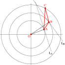
Figure 4: Nice triangle $[A,B,C]$.

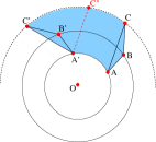
Figure 5: Nicely swept set (NSS, in blue) with $A,B,C$ in CCW order.

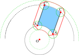
Figure 6: Expansion of $TruncStrip(A,C;A^{\prime},C^{\prime\prime})$ of Fig. 6 (in red).

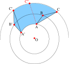
Figure 7: Nicely swept set (NSS, in blue) with $A,B,C$ in CW order.

If $T$ is a nice triangle, then $T[\alpha,\beta]$ is called a nicely swept set (NSS). See  Figure 6, where $T[\alpha,\beta]$ is shaded in blue. Let $T[\alpha]$ be the triangle $[A,B,C]$ and $T[\beta]$ be $[A^{\prime},B^{\prime},C^{\prime}]$. W.l.o.g., assume that $A,B,C$ appear in counter-clockwise (CCW) order as indicated in Figure 6. Then we can subdivide $T[\alpha,\beta]$ into two parts: the triangle $[A,B,C]$ and another part which we call a swept segment.

Notation for Swept Segment: if $S$ is the line segment $[A,C]$, then write $S[\alpha,\beta]$ for this swept segment. The boundary of $S[\alpha,\beta]$ is decomposed into the following sequence of four curves given in clockwise (CW) order: (i) the arc $(A,A^{\prime})$ centered at $O$ of radius $\|A\|$ from $A$ to $A^{\prime}$, (ii) the segment $[A^{\prime},C^{\prime}]$, (iii) the arc $(C^{\prime},C)$ centered at $O$ of radius $\|C\|$ from $C^{\prime}$ to $C$, (iv) the segment $[C,A]$.

Our next goal is to consider $s$-expansion of the swept segment, i.e.,

$$X=S[\alpha,\beta]\oplus Disc(s).$$ (4)

Specifically, we want an easy way to detect the intersection between this expansion with any given feature (corner or edge). To do so, we want to express $X$ as the union of “basic shapes.” A subset of ${\mathbb{R}}^{2}$ is a $0$-basic shape if it is a half-space, a disc or complement of a disc. We write $Disc(r)$ for the disc of radius $r$ centered at $O$, and $Ann(r,r^{\prime})$ for the annulus with inner radius $r$ and outer radius $r^{\prime}$ centered at $O$. A shape $X$ is said to be $1$-basic if it can be written as the finite intersection $X=\bigcap_{j=1}^{k}X_{j}$ where $X_{j}$’s are $0$-basic shapes. The $1$-size of $X$ is the minimum $k$ in such an intersection. So polygons with $n$ sides have $1$-size of $n$. Truncated triangular sets have $1$-size of $4$. We need some other $1$-basic shapes:

• Strips: $Strip(a,b;a^{\prime},b^{\prime})$ is the region between the two parallel lines $\overline{a,b}$ and $\overline{a^{\prime},b^{\prime}}$. Here $a,b,a^{\prime},b^{\prime}$ are distinct points.

• Truncated strips: $TruncStrip(a,b;a^{\prime},b^{\prime})$ is the intersection of $Strip(a,b;a^{\prime},b^{\prime})$ with an annulus; the boundary of this shape is comprised of two line segments $[a,b]$ and $[a^{\prime},b^{\prime}]$ and two arcs $(a,a^{\prime})$ and $(b,b^{\prime})$ from the boundary of the annulus.

• Sectors: $Sector(a,b,b^{\prime})$ denotes any region bounded by a circular arc $(b,b^{\prime})$ and two segments $[a,b]$ and $[a,b^{\prime}]$.

Finally, a shape $X$ is said to be $2$-basic if it can be written as a finite union of $1$-basic shapes, $X=\bigcup_{j=1}^{m}X_{j}$ where $X_{j}$’s are $1$-basic. We call $\left\{X_{1},\ldots,X_{m}\right\}$ a basic representation of $X$. The $2$-size of the representation is the sum of the $1$-sizes of $X_{j}$’s. Thus, for any box $B^{t}\subseteq{\mathbb{R}}^{2}$, the $s$-expansion of $B^{t}$ is a $2$-basic shape since it is the union of four discs and an octagon. We now consider the case where $X$ is the $s$-expansion of a swept segment $S[\alpha,\beta]$. We first decompose $S[\alpha,\beta]$ into two shapes as follows: suppose $C^{\prime\prime}$ lies on the circle of radius $\|C\|=\|C^{\prime}\|$. Considering both cases of $A,B,C$ being in CCW and CW orders, there are two possible representations:
(1) If $[A^{\prime},C^{\prime\prime}]$ is parallel to $[A,C]$ and $[A^{\prime},C^{\prime\prime}]\subseteq Ann(\|A\|,\|C\|)$, then we have

$$S[\alpha,\beta]=Sector(A^{\prime},C^{\prime},C^{\prime\prime})\cup TruncStrip(A,C;A^{\prime},C^{\prime\prime}).$$ (5)

(2) If $[A,C^{\prime\prime}]$ is parallel to $[A^{\prime},C^{\prime}]$ and $[A,C^{\prime\prime}]\subseteq Ann(\|A\|,\|C\|)$, then we have

$$S[\alpha,\beta]=Sector(A,C,C^{\prime\prime})\cup TruncStrip(A,C^{\prime\prime};A^{\prime},C^{\prime}).$$ (6)

The swept segment in Figure 6 supports the representation (5) but not (6), while the swept segment in Figure 7 supports the representation (6) but not (5). Note that they are symmetric cases, with $A,B,C$ in CCW order in Figure 6 and in CW order in Figure 7. Also, if the angular range of $[\alpha,\beta]$ is greater than $90$ degrees and the points $O,A,C$ are collinear, then both representations fail! We next show when at least one of the representations succeeds:

Lemma 4

Assume the width of the angular range $[\alpha,\beta]$ is at most $\pi/2$. Then swept segment $S[\alpha,\beta]$ can be decomposed into a sector and a truncated strip as in (5) or (6).

Clearly, the $s$-expansion of a sector is $2$-basic. This is also true for truncated strips (w.l.o.g., considering that in the representation (5)):

Lemma 5

Let $X=TruncStrip(A,C;A^{\prime},C^{\prime\prime})$. There is a basic representation of $X\oplus D(s)$ of the form $\left\{D_{1},D_{2},D_{3},D_{4},X^{\prime}\right\}$ where $D_{i}$’s are discs and $X^{\prime}$ is the intersection of a convex hexagon with an annulus.

Combining all these lemmas, we conclude:

Theorem 6

Let $T[\alpha,\beta]$ be a nicely swept set where $[\alpha,\beta]$ has width $\leq\pi/2$. Then $T[\alpha,\beta]$ can be decomposed into a triangle, a sector and a truncated strip. The $s$-expansion of $T[\alpha,\beta]$ has a basic representation which is the union of the $s$-expansions of the triangle, sector and truncated strip.

The complexity of testing intersection of $2$-basic shapes with any feature is proportional to its $2$-size, which is $O(1)$. This theorem assures us that the constants in “$O(1)$” is small. Note that it is not correct to test if a line segment $L$ intersects a $1$-basic shape $X=\bigcap_{j=1}^{k}X_{j}$ by just testing if $L$ intersects every $X_{j}$, since $L$ could intersect every $X_{j}$ but not all in the same place(s) so that $L\cap X=\emptyset$. Therefore, we need to maintain the common intersections between $L$ and all $X_{j}$’s tested so far as we loop over all $X_{j}$’s; at the end, $L$ intersects $X$ if and only if there is at least one non-empty set of common intersections. Since the complement of a disk is non-convex, in general this process could result in many sets/segments of common intersections to maintain. Fortunately, there is at most one complement of a disk in our decomposition of an $NSS$. Thus it is enough to maintain just a single set/segment of the common intersection of $L$ with all other $0$-basic shapes, and check with the complement of a disk only at the end.

4.2 Partitioning an $n$-gon into Nice Triangles

Suppose $P$ is an $n$-gon. We can partition it into $n-2$ triangles. W.l.o.g., there is at most one triangle that contains the origin $O$. We can split that triangle into at most 6 nice triangles, using our technique for star-shaped polygons (Lemma 2).

Lemma 7

If $T$ is an arbitrary triangle and $O$ is exterior to $T$, then we can partition $T$ into at most $4$ nice triangles.

The number $4$ in this lemma is the best possible: if $T$ is a triangle with circumcenter $O$, then any partition of $T$ into nice triangles would have at least $4$ triangles because we need to introduce vertices in the middle of each side of $T$.

Theorem 8

Let $P$ be an $n$-gon.
(i) Given any triangulation of $P$ into $n-2$ triangles, we can refine the triangulation into a triangulation with $\leq 4n-6$ nice triangles.
(ii) This bound is tight in this sense: for every $n\geq 3$, there is a triangulation of $P$ whose refinement has size $4n-6$.  

4.3 Soft Predicates and T/R Subdivision Scheme

We can now follow the same paradigm as for star-shaped robots in Sec. 3.2. We first apply Theorem 8(i) to partition the robot $R_{0}$ into a set of nice triangles, $R_{0}=\cup_{j}T_{j}$, where all $T_{j}$’s share a common origin $O$, and we will use the soft predicates developed for $T_{j}$ and apply Proposition A. The origin $O$ plays a similar role as the apex in Sec. 3.2. The T/R splitting scheme is exactly the same: we first perform T-splits, splitting only the translational boxes until they are $\varepsilon$-small, and then we perform R-splits, splitting only the rotational boxes until they are $\varepsilon$-small. Essentially the top part of the subdivision tree is a quad-tree, and the bottom parts are binary subtrees (see Sec. 3.2).

The feature set for a subdivision box $B$ where we perform T-splits is the same as before; the only difference is that now for a box $B$ where we perform R-splits, we use a new feature set $\widetilde{\phi}_{j}(B)$ for each nice triangle $T_{j}$ where $O$ is not at its vertex (there are at most 6 nice triangles with $O$ at a vertex/apex; see Theorem 8(i)). Suppose $T_{j}=[a,b,c]$ with $0\leq\|a\|\leq\|b\|\leq\|c\|$. Let $r_{j}=\|c\|$. Also, suppose the angle range of box $B=(B^{t},B^{r})$ is $B^{r}=[\theta_{1},\theta_{2}]$. Recall the footprint of $T_{j}[\theta_{1},\theta_{2}]$ is a nicely swept set (NSS); denote it $NSS_{j}$. Then the new feature set $\widetilde{\phi}_{j}(B)$ for $T_{j}$ comprises those $f$ where $\mathrm{Sep}(m_{B},f)\leq r_{B}+r_{j}$ and $f$ also intersects the $r_{B}$-expansion of $NSS_{j}$ (where $m_{B}$ and $r_{B}$ are the midpoint and radius of $B$).

5 Experimental Results

Table 1: Robot Statistics.

Robot	$m$ (# sides)	$t$ (# triangles)
L-shaped	6	4
snowflake	18	24
S-shaped	12	26
3-legged	14	20
C-shaped	18	22

Table 2: Running Our Planner (R: radius of the robot’s circumcircle around its rotation center; P?: path found? (Yes/No); Time is in s; S-shaped*: thin version).

Exp#	Robot	Envir.	R	$\epsilon$	$\alpha$	$\beta$	P?	Time
0	L-shaped	gateway	50	2	(18, 98, 340∘)	(458,119,270∘)	Yes	10.106
1	L-shaped	gateway	50	4	(18, 98, 340∘)	(458,119,270∘)	No	8.431
2	snowflake	sparks	56	2	(108, 136, 0∘)	(358, 155, 0∘)	Yes	17.846
3	snowflake	sparks	56	2	(108, 136, 0∘)	(358, 155, 180∘)	Yes	3.370
4	S-shaped	sparks	74	4	(132, 80, 90∘)	(333, 205, 90∘)	Yes	34.284
5	S-shaped	sparks	74	4	(132, 80, 90∘)	(333, 205, 60∘)	No	57.371
6	3-legged	sparks	70	2	(108, 136, 0∘)	(368, 155, 0∘)	Yes	41.745
7	L-shaped	corridor	68	2	(75, 420, 0∘)	(370, 420, 0∘)	Yes	4.012
8	L-shaped	corridor	68	3	(75, 420, 0∘)	(370, 420, 0∘)	Yes	1.926
9	L-shaped	corridor	68	5	(75, 420, 0∘)	(370, 420, 0∘)	Yes	2.684
10	L-shaped	corridor-L	68	5	(75, 420, 0∘)	(370, 420, 0∘)	No	2.908
11	L-shaped	corridor-L	68	3	(75, 420, 0∘)	(370, 420, 0∘)	Yes	2.255
12	C-shaped	corridor-S	80	4	(80, 450, 0∘)	(380, 450, 0∘)	Yes	26.200
13	S-shaped	maze	38	2	(38, 38, 0∘)	(474, 474, 90∘)	No	90.097
14	S-shaped*	maze	38	2	(38, 38, 0∘)	(474, 474, 90∘)	Yes	79.518

Table 3: Comparing with OMPL (“#”: Exp#; “Time/P?”: our run time (in s)/path found? (Y/N). Each OMPL method: Average Time (in s)/Standard Deviation/Success Rate, over 10 runs).

#	Time/P?	PRM	RRT	EST	KPIECE
0	10.106/Y	4.18/2.53/1	42.13/38.49/1	76.22/110.44/0.9	300/0/0
2	17.846/Y	9.22/6.82/1	210.41/144.25/0.3	271.75/89.31/0.1	240.00/126.47/0.2
3	3.370/Y	300/0/0	300/0/0	300/0/0	300/0/0
4	34.284/Y	5.93/7.20/1	217.33/134.53/0.3	300/0/0	300/0/0
5	57.371/N	300/0/0	300/0/0	300/0/0	300/0/0
6	41.745/Y	2.72/4.89/1	154.22/141.77/0.5	104.32/78.10/0.7	3.16/4.28/1
8	1.926/Y	0.63/0.55/1	300/0/0	3.02/4.71/1	0.41/0.28/1
11	2.255/Y	1.49/0.84/1	300/0/0	241.24/124.88/0.2	1.58/1.47/1
12	26.200/Y	3.16/4.21/1	300/0/0	172.506/120.38/0.7	93.88/88.03/0.8
13	90.097/N	300/0/0	300/0/0	300/0/0	300/0/0
14	79.518/Y	300/0/0	236.72/106.44/0.3	300/0/0	39.81/91.57/0.9

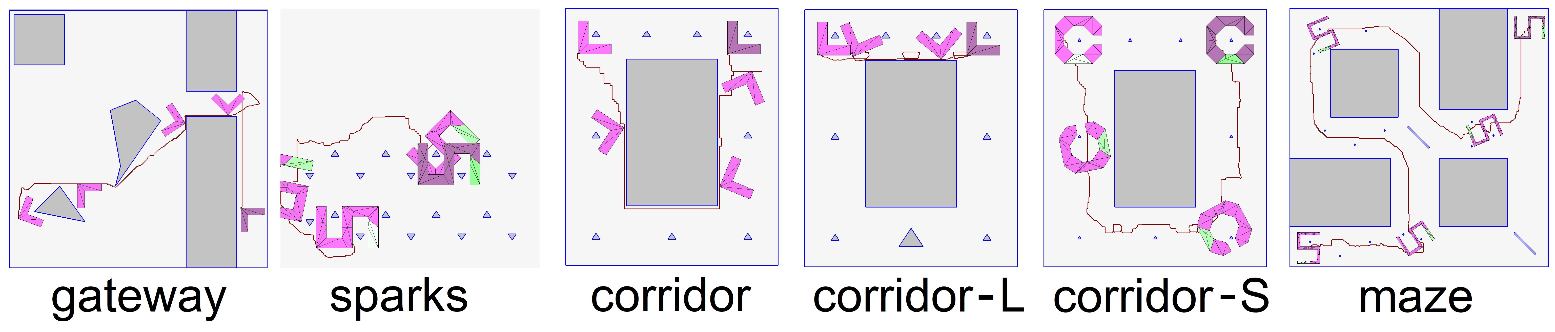
Figure 8: Six Environments in our experiments.

We have implemented our approaches in C/C++ with Qt GUI platform. The software and data sets are freely available from the web site for our open-source Core Library [6]. All experiments are reproducible as targets of Makefiles in Core Library. Our experiments are on a PC with one 3.4GHz Intel Quad Core i7-2600 CPU, 16GB RAM, nVidia GeForce GTX 570 graphics and Linux Ubuntu 16.04 OS. The results are summarized in Table 2 and Table 3. Table 2 is concerned only with the behavior of our complex robots; Table 3 gives comparisons with the open-source OMPL library [14]. The robots are as shown in Figure 2; their statistics are given in Table 1.

We select some interesting experiments to analyze characteristic behavior of our planner. Please see Table 2 and the video ( https://cs.nyu.edu/exact/gallery/complex/complex-robot-demo.mp4). In Exp0-1, we show how the parameter $\epsilon$ affects the result. With a narrow gateway, when we change $\epsilon$ from $2$ to $4$, the output changes from a path to NO-PATH for the same configuration. In Exp2-3, we observe how the snowflake robot rotates and maneuvers to get from the start to two different goals. For Exp4-5, the difference is in the angles of the goal configuration; in Exp5 this is designed to be an isolated configuration and the planner outputs NO-PATH  as desired. Exp6 shows how the robot squeezes among the obstacles to move its complex shape through the environment. Exp7-9 use the same L-shaped robot, $\alpha,\beta$ configurations and the environment; only $\epsilon$ varies. The planner can find three totally different paths. When $\epsilon$ is small (Exp7), the path is very carefully adjusted to move the robot around the obstacles. When $\epsilon$ is larger (Exp8), the planner finds an upper path with a higher clearance. When $\epsilon$ is even larger (Exp9), the planner chooses a very safe but much longer path at the bottom. Note that using a larger $\epsilon$ usually makes the search faster, since we stop splitting boxes smaller than $\epsilon$, but a longer path can make the search slower. In Exp10-11, we modify the environment of Exp7-9 by putting a large obstacle at the bottom, which forces the robot to find a path at the top. Exp12 uses an environment similar to those in Exp7-11 but with much smaller scattered obstacles. It is designed for the C-shaped robot, which can rotate while having an obstacle in its pocket. Exp13-14 use a challenging environment where the small scattered obstacles force the S-shaped robot to rotate around and only the “thin” version (Exp14, also in Fig. 8 “maze”) can squeeze through.

In Table 3 we compare our planner with several sampling algorithms in OMPL: PRM, RRT, EST, and KPIECE. These experiments are correlated to those in Table 2 (see the Exp #). Each OMPL planner is run 10 times with a time limit 300 seconds (default), where all planner-specific parameters use the OMPL default values. We see that for OMPL planners there are often unsuccessful runs and they have to time out even when there is a path. On the other hand, our algorithm consistently solves the problems in a reasonable amount of time, often much faster than the OMPL planners, in addition to being able to report NO-PATH.

6 Conclusions

Although the study of rigorous algorithms for motion planning has been around for over 40 years, there has always been a gap between such theoretical algorithms and the practical methods. Our introduction of resolution-exactness and soft predicates on the theoretical front, together with matching implementations, closes this gap. Moreover, it eliminated the “narrow passage” problem that plagued the sampling approaches. The present paper extends our approach to challenging planning problems for which no exact algorithms exist.

What are the current limitations of our work? We implement everything in machine precision (the practice in this field). But it can be easily modified to achieve the theoretical guarantees of resolution-exactness if we use arbitrary precision BigFloats number types.

We pose two open problems: One is to find an optimal decomposition of $m$-gons into nice triangles (currently, we simply give an upper bound). Such decompositions will have impact for practical complex robots. Second, we would like to develop similar decomposability of soft predicates for complex rigid robots in ${\mathbb{R}}^{3}$.

APPENDIX: Proofs

Lemma 1. Let $T$ be a pointed triangular set. Then $T$ is nice iff for all $\alpha\in S^{1}$ ($0<\alpha<\pi-a$), the footprints $T[0,\alpha]$ and $T[-\alpha,0]$ are truncated triangular sets (TTS).

Proof. If $T$ is nice, $T[0,\alpha]$ and $T[-\alpha,0]$ are truncated triangular sets (TTS); this is easily seen in Figure 3(c).

Conversely, if $T$ is not nice, let us assume that $\|A-B\|\leq\|A-C\|$ (e.g., Figure 3(d)). We claim that for sufficiently small $\alpha>0$, either $T[0,\alpha]$ or $T[-\alpha,0]$ is not a TTS. Assume (w.l.o.g.) that $A,B,C$ are in CCW order; we show that $T[0,\alpha]$ is not a TTS.

If $T$ is not nice, then $b<90^{\circ}$. Let $B-C$ intersects the $CircleB$ (the circle centered at $A$ that passes through $B$) at $D$. Let $\alpha_{max}=\angle BAD=180^{\circ}-2b=2(90^{\circ}-b)$, since $b=\angle ABD=\angle ADB$. Note that a TTS is a convex set as it is the intersection of three half-spaces and one disc; all of them are convex and thus the intersection is also convex. However, for any $\alpha<\alpha_{max}$, $T[0,\alpha]$ is not a TTS since $B-C$ will intersect $B^{\prime}-C^{\prime}$ inside $CircleB$ (see Figure 9) — this makes $T[0,\alpha]$ non-convex and thus it is not a TTS.   $\Box$

\begin{picture}(11249.0,5795.0)(676.0,-6006.0)\end{picture}

Figure 9: Proof of Lemma 1: $T[0,\alpha]$ is not a truncated triangular set (TTS).

Lemma 2. Let $R_{0}$ be a star-shaped polygonal region with $A$ as center. If the boundary of $R_{0}$ is an $n$-gon, then we can decompose $R_{0}$ into an essentially disjoint union of at most $2n$ bounded triangular sets (i.e., at most $2n$ triangles) that are nice and have $A$ as the apex.

Proof. First, for each vertex $v$ of $R_{0}$ we add a segment connecting $A$ and $v$. This decomposes $R_{0}$ into a disjoint union of $n$ triangles (since $R_{0}$ is star-shaped). Now consider each of the resulting triangle $T=[A,B,C]$ and let $A$ be the apex of $T$. If $T$ is not nice, then both angles $b$ and $c$ (corresponding to vertices $B$ and $C$) are less than $90^{\circ}$, and we can add a segment $[A,D]$ that is perpendicular to edge $[B,C]$ and intersects $[B,C]$ at $D$ where $D$ is in the interior of $[B,C]$. This effectively decomposes $T$ into two nice triangles $[A,D,B]$ and $[A,D,C]$ with $A$ being the common apex. In this way, we can decompose $R_{0}$ into at most $2n$ nice triangles that have $A$ as the apex.   $\Box$

Lemma 4. Assume the width of the angular range $[\alpha,\beta]$ is at most $\pi/2$. Then swept segment $S[\alpha,\beta]$ can be decomposed into a sector and a truncated strip as in (5) or (6)

Proof. Our goal is to choose the point $C^{\prime\prime}$ so that either (5) or (6) holds. Let the swept segment be $S[\alpha,\beta]$, with $S[\alpha]=[A,C]$ and $S[\beta]=[A^{\prime},C^{\prime}]$. Let $D$ (resp., $D^{\prime}$) be the point such that $\|D\|=\|C\|$ (resp., $\|D^{\prime}\|=\|C\|$) and $O,A,D$ (resp., $O,A^{\prime},D^{\prime}$) are collinear. Then $Sector(O,D,D^{\prime})$, bounded by the arc $(D,D^{\prime})$ centered at $O$, contains either $[A,C]$ or $[A^{\prime},C^{\prime}]$. If it contains $[A,C]$ (see Figure 6), then we choose $C^{\prime\prime}$ such that $[A^{\prime},C^{\prime\prime}]\subseteq Sector(O,D,D^{\prime})$ and $[A,C]$ is parallel to $[A^{\prime},C^{\prime\prime}]$, and thus (5) holds. By symmetry, if the sector contains $[A^{\prime},C^{\prime}]$ (see Figure 7), we can choose $C^{\prime\prime}$ so that (6) holds.   $\Box$

Lemma 5. Let $X=TruncStrip(A,C;A^{\prime},C^{\prime\prime})$. There is a basic representation of $X\oplus D(s)$ of the form $\left\{D_{1},D_{2},D_{3},D_{4},X^{\prime}\right\}$ where $D_{i}$’s are discs and $X^{\prime}$ is the intersection of a convex hexagon with an annulus.

Proof. See Figure 6 for a figure of $X$. Let $D_{1}=Disc_{A},D_{2}=Disc_{C},D_{3}=Disc_{A^{\prime}},D_{4}=Disc_{C^{\prime\prime}}$ where $Disc_{P}$ denote the disc with center $P$ of radius $s$. These discs are outlined in green in Figure 6. The boundary of each $D_{i}$ ($i=1,\ldots,4$) intersects the boundary of $X\oplus D(s)$ in a circular arc $(a_{i},b_{i})$ where $a_{i}$ is closer to $O$ than $b_{i}$. Let $H_{i}$ be the half space containing $X$ and bounded by the line through $[a_{i},b_{i}]$. We need to check that these half spaces do indeed contain $X$. Also, let $H_{5}$ (resp., $H_{6}$) be the half space containing $X$ and bounded by the line through $b_{1}$ and $a_{2}$ (resp., $b_{3}$ and $a_{4}$). Note that $[b_{1},a_{2}]$ and $[b_{3},a_{4}]$ are parallel. Then we see that $H=\bigcap_{i=1}^{6}H_{i}$ is a convex hexagon containing $X$, and the intersection $H\cap Ann(\|A\|-s,\|C\|+s)$ is outlined in red in Figure 6. Observe that this intersection covers all of $\Big{(}X\oplus Disc(s)\Big{)}\setminus\bigcup_{i=1}^{4}D_{i}$.

This construction is valid as long as $\|A\|\geq s$, i.e., the annulus $Ann(\|A\|-s,\|C\|+s)$ is a true annulus. When $\|A\|<s$, the boundary of $X\oplus Disc(s)$ no longer has an inner arc of radius $\|A\|-s$, but degenerates into a concave vertex where the two circles of radius $s$ centered at $A$ and $A^{\prime}$ (resp.) meet.   $\Box$

Theorem 6. Let $T[\alpha,\beta]$ be a nicely swept set where $[\alpha,\beta]$ has width $\leq\pi/2$. Then $T[\alpha,\beta]$ can be decomposed into a triangle, a sector and a truncated strip. The $s$-expansion of $T[\alpha,\beta]$ has a basic representation which is the union of the $s$-expansions of the triangle, sector and truncated strip.

Proof. We know that $T[\alpha,\beta]$ can be decomposed into a triangle and a swept segment. The swept segment, since $[\alpha,\beta]$ has width $\leq\pi/2$, can be further decomposed into a sector and a truncated strip. The expansions of the triangle and sector are clear; the expansion of the truncated strip was the subject of the previous lemma.   $\Box$

Lemma 7. If $T$ is an arbitrary triangle and $O$ is exterior to $T$, then we can partition $T$ into at most $4$ nice triangles.

Proof. Let $T=[A,B,C]$. In the worst case, all three niceness conditions for $T$ (i.e., $B\in H_{A},C\in H_{A}$, and $C\in H_{B}$, where $0\leq\|A\|\leq\|B\|\leq\|C\|$; recall the geometric view of niceness described right after Eq. (3)) are violated. W.l.o.g., suppose that among the three edges of $T$, $[A,B]$ is the closest to $O$. Let $D$ be the point on $[A,B]$ such that $[O,D]\perp[A,B]$, and similarly for $E\in[A,C]$ and $F\in[B,C]$; see Figure 10. Then we add segments $[C,D],[D,E],[D,F]$ to decompose $T$ into 4 triangles $[D,E,A],[D,E,C],[D,F,B]$ and $[D,F,C]$. Note that the line $L_{D}$ tangent to the circle of radius $\|D\|$ (centered at $O$) and passing through the point $D$ coincides with $[A,B]$; similarly, the line $L_{E}$ coincides with $[A,C]$ and $L_{F}$ coincides with $[B,C]$. As before, $H_{D}$ is the half space bounded by $L_{D}$ and not containing $O$; similarly for $H_{E}$ and $H_{F}$. For the triangle $[D,E,A]$, note that $0\leq\|D\|\leq\|E\|\leq\|A\|$ since $[A,B]$ is closer to $O$ than $[A,C]$ (so $\|D\|\leq\|E\|$), $[O,D]\perp[D,A]$ (so $\|D\|\leq\|A\|$) and $[O,E]\perp[E,A]$ (so $\|E\|\leq\|A\|$). Thus the three niceness conditions for the triangle $[D,E,A]$ are: $E\in H_{D},A\in H_{D}$, and $A\in H_{E}$. Again, these three conditions are satisfied due to the facts that $[A,B]$ is closer to $O$ than $[A,C]$, $[O,D]\perp[D,A]$ and $[O,E]\perp[E,A]$, i.e., these conditions are automatically satisfied due to the construction of $D$ and $E$. Similarly, the three niceness conditions for the triangle $[D,E,C]$ are: $E\in H_{D},C\in H_{D}$, and $C\in H_{E}$, which are again satisfied due to the construction of $D$ and $E$. Symmetrically, the triangles $[D,F,B]$ and $[D,F,C]$ are both nice due to the construction of $D$ and $F$. Therefore $T$ can be decomposed into at most 4 nice triangles.

$\Box$

\begin{picture}(6015.0,3510.0)(976.0,-3496.0)\end{picture}

Figure 10: Proof of Lemma 7: A triangle $T=[A,B,C]$ with the origin $O$ in the exterior can be decomposed into at most 4 nice triangles.

Theorem 8. Let $P$ be an $n$-gon.
(i) Given any triangulation of $P$ into $n-2$ triangles, we can refine the triangulation into a triangulation with $\leq 4n-6$ nice triangles.
(ii) This bound is tight in this sense: for every $n\geq 3$, there is a triangulation of $P$ whose refinement has size $4n-6$.

Proof. (i) In the given triangulation of $P$, we might have a triangle containing $O$. This triangle can be triangulated into at most $6$ nice triangles (Lemma 2). By Lemma 7, the remaining $n-3$ triangles can be refined into $4(n-3)$ nice triangles. The final count is $6+4(n-3)=4n-6$.

(ii) We construct an $n$-gon whose vertices are all on the unit circle. Note that all such vertices are of the form $e^{\mbox{\bf i}\theta}$. For the first triangle $T_{0}$, pick the vertices $1,e^{\mbox{\bf i}2\pi/3},e^{\mbox{\bf i}4\pi/3}$. Call these vertices $u_{0},u_{1},u_{2}$. Choose the origin $O$ inside $T_{0}$ so that for each triangle $[O,u_{i},u_{j}],i\neq j\in\left\{0,1,2\right\}$ we have both $\angle Ou_{i}u_{j}<90^{\circ}$ and $\angle Ou_{j}u_{i}<90^{\circ}$. Therefore each triangle $[O,u_{i},u_{j}]$ must be split into $2$ nice triangles and overall $T_{0}$ must be split into $6$ nice triangles. If $n=3$, our result is verified. If $n>3$, we must add $n-3$ additional vertices. Define the vertex $v_{k}{\color[rgb]{1,0,0}\mathrel{\,:=\,}}e^{\mbox{\bf i}\frac{2k\pi}{3(n-2)}}$, $k=0,1,\ldots,n-2$ (note that $v_{0}=1$ and $v_{n-2}=e^{\mbox{\bf i}2\pi/3}$ have previously been chosen). Thus we have added $v_{1},\ldots,v_{n-3}$ new vertices. Any triangle $[v_{k},v_{\ell},v_{m}]$ must be split into $4$ nice triangles. This proves our claim.   $\Box$

References

- [1] F. Avnaim, J.-D. Boissonnat, and B. Faverjon. A practical exact motion planning algorithm for polygonal objects amidst polygonal obstacles. In B. J.D. and L. J.P., editors, Geometry and Robotics, LNCS Vol 391. Springer, Berlin-Heidelberg, 1989.
- [2] M. Barbehenn and S. Hutchinson. Efficient search and hierarchical motion planning by dynamically maintaining single-source shortest paths trees. IEEE Trans. Robotics and Automation, 11(2), 1995.
- [3] J. Basch, L. Guibas, D. Hsu, and A. Nguyen. Disconnection proofs for motion planning. In IEEE Int’l Conf. on Robotics Animation, pages 1765–1772, 2001.
- [4] H. Bennett, E. Papadopoulou, and C. Yap. Planar minimization diagrams via subdivision with applications to anisotropic Voronoi diagrams. Eurographics Symposium on Geometric Processing, 35(5), 2016. SGP 2016, Berlin, Germany. June 20-24, 2016.
- [5] H. Choset, K. M. Lynch, S. Hutchinson, G. Kantor, W. Burgard, L. E. Kavraki, and S. Thrun. Principles of Robot Motion: Theory, Algorithms, and Implementations. MIT Press, Boston, 2005.
- [6] Core Library. https://cs.nyu.edu/exact/core_pages/downloads.html.
- [7] D. Halperin, E. Fogel, and R. Wein. CGAL Arrangements and Their Applications. Springer-Verlag, Berlin and Heidelberg, 2012.
- [8] C.-H. Hsu, Y.-J. Chiang, and C. Yap. Rods and rings: Soft subdivision planner for R^3 x S^2. In Proc. 35th Int’l Symp. on Comp. Geom.(SoCG 2019), June 18-21, 2019. To appear. CG Week 2019, Portland Oregon. Also in arXiv:1903.09416.
- [9] J.-C. Latombe. Robot Motion Planning. Kluwer Academic Publishers, 1991.
- [10] S. M. LaValle. Planning Algorithms. Cambridge University Press, Cambridge, 2006.
- [11] Z. Luo, Y.-J. Chiang, J.-M. Lien, and C. Yap. Resolution exact algorithms for link robots. In Proc. 11th Intl. Workshop on Algorithmic Foundations of Robotics (WAFR ’14), volume 107 of Springer Tracts in Advanced Robotics (STAR), pages 353–370, 2015. Aug. 3-5, 2014, Boǧazici University, Istanbul, Turkey.
- [12] V. Milenkovic, E. Sacks, and S. Trac. Robust complete path planning in the plane. In Proc. 10th Workshop on Algorithmic Foundations of Robotics (WAFR 2012), Springer Tracts in Advanced Robotics, vol.86, pages 37–52. Springer, 2012.
- [13] O. Salzman, M. Hemmer, B. Raveh, and D. Halperin. Motion planning via manifold samples. In Proc. European Symp. Algorithms (ESA), pages 493–505, 2011.
- [14] I. Şucan, M. Moll, and L. Kavraki. The Open Motion Planning Library. IEEE Robotics & Automation Magazine, 19(4):72–82, 2012. http://ompl.kavrakilab.org.
- [15] C. Wang, Y.-J. Chiang, and C. Yap. On soft predicates in subdivision motion planning. Comput. Geometry: Theory and Appl. (Special Issue for SoCG’13), 48(8):589–605, Sept. 2015.
- [16] C. Yap. Soft subdivision search in motion planning. In A. Aladren et al., editor, Proc. 1st Workshop on Robotics Challenge and Vision (RCV 2013), 2013. Robotics Science and Systems Conf. (RSS 2013), Berlin. In arXiv:1402.3213. Full paper: http://cs.nyu.edu/exact/papers/.
- [17] C. Yap. Soft subdivision search and motion planning, II: Axiomatics. In Frontiers in Algorithmics, volume 9130 of Lecture Notes in Comp. Sci., pages 7–22. Springer, 2015. Plenary talk at 9th FAW. Guilin, China. Aug. 3-5, 2015.
- [18] C. Yap, Z. Luo, and C.-H. Hsu. Resolution-exact planner for thick non-crossing 2-link robots. In Proc. 12th Intl. Workshop on Algorithmic Foundations of Robotics (WAFR ’16), 2016. Dec. 13-16, 2016, San Francisco. The appendix in the full paper (and arXiv from http://cs.nyu.edu/exact/ (and arXiv:1704.05123 [cs.CG]) contains proofs and additional experimental data.
- [19] L. Zhang, Y. J. Kim, and D. Manocha. Efficient cell labeling and path non-existence computation using C-obstacle query. Int’l. J. Robotics Research, 27(11–12):1246–1257, 2008.
- [20] B. Zhou, Y.-J. Chiang, and C. Yap. Soft subdivision motion planning for complex planar robots. In Proc. 26th European Symposium on Algorithms (ESA 2018), pages 73:1–73:14, 2018. Helsinki, Finland, Aug. 20-24, 2018.
- [21] D. Zhu and J.-C. Latombe. New heuristic algorithms for efficient hierarchical path planning. IEEE Transactions on Robotics and Automation, 7:9–20, 1991.