Geometric band properties in strained monolayer transition metal dichalcogenides using simple band structures

Abstract

Monolayer transition metal dichalcogenides (TMDs) bare large Berry curvature hotspots readily exploitable for geometric band effects. Tailoring and enhancement of these features via strain is an active research direction. Here, we consider spinless two- and three-band, and spinful four-band models capable to quantify Berry curvature and orbital magnetic moment of strained TMDs. First, we provide a $k\cdot p$ parameter set for MoS₂, MoSe₂, WS₂, and WSe₂ in the light of the recently released ab initio and experimental band properties. Its validity range extends from $K$ valley edge to about hundred millielectron volts into valence and conduction bands for these TMDs. To expand this over a larger part of the Brillouin zone, we incorporate strain to an available three-band tight-binding Hamiltonian. With these techniques we demonstrate that both the Berry curvature and the orbital magnetic moment can be doubled compared to their intrinsic values by applying typically a 2.5% biaxial tensile strain. These simple band structure tools can find application in the quantitative device modeling of the geometric band effects in strained monolayer TMDs.

I Introduction

The monolayer transition metal dichalcogenides (TMDs) of the semiconducting $2H$ polytype avail wide range of electrical, magnetic, optical, and mechanical control and tunability. Xu et al. (2014); Manzeli et al. (2017); Mak, Xiao, and Shan (2018) Their valley-contrasting properties associated with the so-called inequivalent $K$ valleys at the corners of hexagonal Brillouin zone grant information carriers the opportunity to experience non-dissipative electronics. Yamamoto et al. (2015) Unlike the similar multiple conduction band valleys in conventional bulk silicon electronics, in TMDs the valley degree of freedom is practically an individually accessible quantum label. Schaibley et al. (2016) For instance, in the so-called valley Hall effect an in-plane electric field initiates a valley current in the transverse in-plane direction, Xiao, Yao, and Niu (2007); Yao, Xiao, and Niu (2008); Xiao et al. (2012) which has been confirmed by both optical Mak et al. (2014) and transport Wu et al. (2019) measurements.

At the heart of these valley-based physics there lies the sublattice-driven orbital angular momentum. Yao, Xiao, and Niu (2008); Cao et al. (2012) Alternatively, from the perspective of quantum geometrical band properties, Vanderbilt (2018) the foregoing effects can be attributed to the Berry curvature (BC) and orbital magnetic moment (OMM). Xiao, Chang, and Niu (2007) Both of them take part in various phenomena such as the dichroic selection rules in optical absorption, Zhang, Shan, and Xiao (2018); Cao, Wu, and Louie (2018) or the excitonic $p$ level energy splitting which is proportional to the BC flux; Srivastava and Imamoğlu (2015); Zhou et al. (2015) OMM accounts for the interatomic currents (self-rotating motion of the electron wavepacket) Chang and Niu (2008) responsible for the valley $g$-factor in TMDs. Brooks and Burkard (2017); Rybkovskiy, C.Gerber, and Durnev (2017) Thus, by breaking time-reversal symmetry with a perpendicular magnetic field, a valley Zeeman splitting is introduced in addition to the well-known spin Zeeman effect. Aivazian et al. (2015); Srivastava et al. (2015) Very recently, through their intimate connection with the orbital angular momentum, these geometric band properties are locally mapped in momentum space using circular dichroism angle-resolved photoelectron spectroscopy. Schüler et al. (2019)

A unique advantage of TMDs is their mechanical deformability up to at least 10% in their lattice constants without degradation.Bertolazzi, Brivio, and Kis (2011) Undoubtedly it is bound to have ramifications on the quantum geometric band properties, where a quantification inevitably necessitates band structure tools reliable under strain. The $k\cdot p$ method has been the first resort because of its simplicity, starting with grapheneXiao, Yao, and Niu (2007) and carried over to other two-dimensional materials. Kormányos et al. (2015); Rostami et al. (2015); Pearce, Mariani, and Burkard (2016); Sevik et al. (2017); Rybkovskiy, C.Gerber, and Durnev (2017) Very recently a strained parametrization is also offered, Fang et al. (2018a) which we used to successfully explain the experimental photoluminescence peak shifts in strained TMDs. Aas and Bulutay (2018) On the other hand, it has a number of shortcomings especially for studying carrier transport away from the $K$ point. Namely, it is isotropic, preserves the electron-hole symmetry, and remains parabolic. In contrast, TMDs possess the trigonal warping (TW) of the isoenergy contours which leads to measurable effects in the polarization of electroluminescence in p-n junctions. Zhang et al. (2014) The electron-hole symmetry breaking has been confirmed by magnetoluminescence experiments. Li et al. (2014); MacNeill et al. (2015) Lastly, the bands quickly display nonparabolic dependence away from the valley minimum Kormányos et al. (2013) which among other quantities directly affects the BC and OMM. Chen et al. (2019)

Another prevailing band structure choice is the tight-binding model for which a number of parametrizations exist for monolayer TMDs. Bromley, Murray, and Yoffe (1972); Cappelluti et al. (2013); Liu et al. (2013); Rostami et al. (2015); Fang et al. (2018b, a) Compared to $k\cdot p$ their agreement with first-principles data is over much wider range of the Brillouin zone, which comes at a price of some added formulation complexity and larger number of fitting parameters. Among these, arguably the simplest to use is the one by Liu et al. which is unfortunately only available for unstrained TMDs. Liu et al. (2013) It should be noted that both $k\cdot p$ and tight-binding models warrant analytically tractable transparent physics. In the literature there is also a vast amount of density functional theory (DFT) based results Rybkovskiy, C.Gerber, and Durnev (2017); Jeong et al. (2018); Zhang et al. (2017); Fang et al. (2018a) which are highly reliable, other than the well known underestimation of the band gap by most DFT exchange-correlation functionals. Rasmussen and Thygesen (2015) This entails further techniques like many-body $GW$ approximation, which yields band gaps much closer to experiments, albeit being computationally very demanding, and so far practically inapplicable to systems beyond a few tens of atoms in the unit cell, Thygesen (2017) making them highly undesirable for device modeling purposes.

The aim of this work is to present simple band structure options that can quantify the changes under strain in the BC and the OMM around a wider portion of the $K$ valleys. For this purpose, to alleviate the drawbacks of existing strained $k\cdot p$ parametrization, such as disagreement with the reported electron and hole effective masses as well as the band gap values, Fang et al. (2018a) we develop two-band spinless and four-band spinful versions taking into account up-to-date first-principles and experimental data including quantum geometrical band properties, as will be described below. The agreement window with the ab initio and tight-binding band structures falls in the range 70-400 meV from the $K$ valley edge for the TMDs targeted in this work: MoS₂, MoSe₂, WS₂, and WSe₂. Moreover, we extend the tight-binding approach by Liu et al. Liu et al. (2013) to uniaxial and biaxial strain conditions. Based on these tools we demonstrate a doubling of BC and OMM for both valence band (VB) and conduction band (CB) under about 2.5% tensile biaxial strain. We also present a simple explanation of how strain modifies these quantum geometrical band properties.

II Theory

II.1 Two-band $k\cdot p$ Hamiltonian

For carriers near the $K$ valley edges of monolayer TMDs, the two-band $k\cdot p$ low-energy Hamiltonian $(H_{0})$ which is dominated by the metal atom’s open $d$ shell orbitals is the starting point of many studies. Xiao et al. (2012) In the presence of strain, characterized by the tensor components $\varepsilon_{ij}$ such that $\{i,j\}\in\{x,y\}$, an extra term $(H_{\varepsilon})$ is introduced. Fang et al. (2018a) These two Hamiltonians are described in the Bloch basis of $\left\{\ket{\bm{k},\,d_{z^{2}}},\,\ket{\bm{k},\,d_{x^{2}-y^{2}}+id_{xy}}\right\}$ by

$$H_{0} = \frac{f_{1}}{2}\sigma_{z}+f_{2}a(k_{x}\sigma_{x}+k_{y}\sigma_{y}),$$ (1)

$$H_{\varepsilon} = f_{4}(\varepsilon_{xx}+\varepsilon_{yy})\sigma_{z}+f_{5}\big{[}(\varepsilon_{xx}-\varepsilon_{yy})\sigma_{x}-2\varepsilon_{xy}\sigma_{y}\big{]},$$ (2)

where $k_{i}$ is the wave vector Cartesian component centered around the corresponding $K$ point, $f$’s are the fitted parameters for different TMD materials, $a$ is the lattice constant and $\sigma_{i}$’s are the Pauli matrix Cartesian components. The expressions in this subsection specifically apply for the $+K$ valley, while those for the $-K$ valley can be obtained by complex conjugation of the matrix entries. Kormányos et al. (2013) Also, we drop the constant midgap position parameters $f_{0}$ and $f_{3}$ in Ref. Fang et al., 2018a, which need to be reinstated in the study of heterostructures for their proper band alignment.

To account for additional features of electron-hole asymmetry, TW, and nonparabolicity we follow Kormányos et al. Kormányos et al. (2013) by including three more terms

$$H_{\mathrm{2B}}(\bm{k})=H_{0}+H_{\varepsilon}+H_{\mathrm{asym}}+H_{\mathrm{TW}}+H_{\mathrm{cubic}},$$ (3)

where,

$$H_{\mathrm{asym}}=\left(\begin{array}[]{cc}\beta k^{2}&0\\ 0&\alpha k^{2}\end{array}\right),$$ (6)

$$H_{\mathrm{TW}}=\kappa\left(\begin{array}[]{cc}0&k_{+}^{2}\\ k_{-}^{2}&0\end{array}\right),$$ (9)

$$H_{\mathrm{cubic}}=\frac{\eta}{2}k^{2}\left(\begin{array}[]{cc}0&k_{-}\\ k_{+}&0\end{array}\right),$$ (12)

and $k_{\pm}=k_{x}\pm ik_{y}$, the parameters $\alpha$ and $\beta$ describe the breaking of the electron-hole symmetry, whereas $\kappa$ is responsible for the TW of the isoenergy contours, and $H_{\mathrm{cubic}}$ serves to improve the fit further away from the $K$ point. Kormányos et al. (2013)

II.2 Three-band tight-binding Hamiltonian

The two-band $k\cdot p$ approach is inevitably restricted to the vicinity of the $K$ points. To extend it over a wider part of the Brillouin zone the number of bands need to be increased considerably.Rybkovskiy, C.Gerber, and Durnev (2017) For the sake of simplicity, we rather prefer the three-band tight-binding (TB) approach which provides a full-zone band structure fitted to the first-principles data, where in the case of up to third nearest neighbor interactions 19 fitting parameters are involved. Liu et al. (2013) It assumes the Bloch basis of $\left\{\ket{\bm{k},\,d_{z^{2}}}\,,\ket{\bm{k},\,d_{xy}}\,,\ket{\bm{k},\,d_{x^{2}-y^{2}}}\right\}$ coming from the atomic orbitals that largely contribute to the VB and CB edges of TMDs. Kormányos et al. (2013) The matrix representation of the Hamiltonian takes the form

$$H_{0}=\left(\begin{array}[]{ccc}V_{0}&V_{1}&V_{2}\\ V_{1}^{*}&V_{11}&V_{12}\\ V_{2}^{*}&V_{12}^{*}&V_{22}\end{array}\right),$$ (13)

where $V_{0},\,V_{1},\,V_{2},\,V_{11},\,V_{12},\,V_{22}$ are the TB matrix elements; for their detailed expressions we refer to Ref. Liu et al., 2013. Though this Hamiltonian is highly satisfactory it is for unstrained TMDs. We remedy this by the two-band deformation potentials proposed by Fang et al. Fang et al. (2018a) that we also use in our $k\cdot p$ theory in Sec. II.1. So, the strain is embodied into the three-band TB Hamiltonian as

$$H_{\varepsilon}=\left(\begin{array}[]{ccc}e_{a}&e_{b}&e_{b}\\ e_{b}&-e_{a}&0\\ e_{b}&0&-e_{a}\end{array}\right),$$ (14)

where

$$e_{a} = f_{4}\left(\varepsilon_{xx}+\varepsilon_{yy}\right),$$ (15)

$$e_{b} = f_{5}\left(\varepsilon_{xx}-\varepsilon_{yy}\right).$$ (16)

Here, our simplistic approach lends itself to a number of restrictions. Even though this TB is a three-band model, the deformation potentials are only available for the two-band case (highest VB and the lowest CB). Fang et al. (2018a) Therefore, we expand it to the two-dimensional subspace formed by $\ket{\bm{k},\,d_{xy}}$ and $\ket{\bm{k},\,d_{x^{2}-y^{2}}}$ which define the highest VB and the first-excited CB around the $K$ valleys, while neglecting the strain coupling between them. Its form (Eq. (14)) complies with the TB $d-d$ sector deformation coupling of monolayer TMDs. Pearce, Mariani, and Burkard (2016) As another remark, here strain only acts through the uniaxial and biaxial components, with no involvement of the shear strain ($\varepsilon_{xy}=\varepsilon_{yx}$). In fact, it has been shown for this level of theory that the latter is only responsible for a rigid shift of the band extrema. Fang et al. (2018a); Aas and Bulutay (2018)

To test the validity of this simple strain extension, in Fig. 1 we compare it with the first-principles band structure results for WSe₂ under $\pm$ 2% biaxial, and unstrained cases. Fang et al. (2018a) As intended, the agreement around the $K$ valley is quite satisfactory, whereas disagreement sets in away from this region especially toward the $\Gamma$ point. Apparently, $\Gamma$ and $K$ valleys have different signs for the deformation potentials causing a direct to indirect transition under compressive strain. Thus, it cannot be represented with only that of a single (i.e., $K$) valley. As a matter of fact, even for the unstrained case the original TB fitting has deficiencies around the $\Gamma$ point. Liu et al. (2013) These limitations will not be of practical concern for this work as the geometrical band properties that we are interested in are localized around the $K$ point, and vanish toward the $\Gamma$ point due to symmetry considerations. Feng et al. (2012)

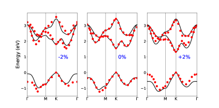
Figure 1: Comparison of first-principles band structure (red dots) Fang et al. (2018a) with the TB results (black line) for WSe₂ under unstrained (0%) and $\pm$ 2% biaxial strain cases. Energy reference is set to VB maximum for each case.

II.3 Berry curvature and orbital magnetic moment

In the absence of an external magnetic field TMDs respect the time reversal symmetry, but inversion symmetry is broken in monolayers or odd number of layers as has been independently confirmed by recent experiments. Mak et al. (2014); Wu et al. (2019) Therefore, in monolayer TMDs BC has a non-zero value with opposite sign in $K$ and $-K$ valleys connected by a time-reversal operation. Xiao, Chang, and Niu (2007) For a chosen band with label $n$ it can be calculated without reference to other bands using

$$\Omega_{n,z}(\bm{k})=-2\,\mathrm{Im}\left\langle\partial_{k_{x}}u_{n{\bm{k}}}|\partial_{k_{y}}u_{n{\bm{k}}}\right\rangle,$$ (17)

where $z$ is the direction perpendicular to monolayer plane, $\ket{u_{n{\bm{k}}}}$ is the cell-periodic part of the Bloch function at wave vector ${\bm{k}}$. Vanderbilt (2018) Another geometric band property is the OMM which is also a pseudovector given by

$$\mu_{n,z}(\bm{k})=2\frac{\mu_{B}m_{0}}{\hbar^{2}}\mathrm{Im}\bra{\partial_{k_{x}}u_{n{\bm{k}}}}\left[H(\bm{k})-E_{n}(\bm{k})\right]\ket{\partial_{k_{y}}u_{n{\bm{k}}}},$$ (18)

where $\mu_{B}$ is the Bohr magneton, $m_{0}$ is the free-electron mass, and $E_{n}(\bm{k})$ is the energy of the band $n$ at the wave vector $\bm{k}$.

II.4 Fitting Procedure and Data References

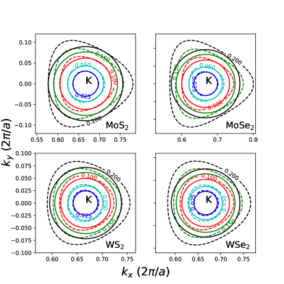
(a)

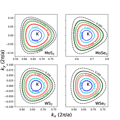
(b)

Figure 2: Isoenergy contours of the VB (at energies indicated in eV) for different TMDs from TB (dashed) and $k\cdot p$ (solid) models, where the latter excludes (a), or includes (b) the TW effect. For these plots, $\Gamma$ point has been taken as the origin for $\bm{k}$.

Our two-band $k\cdot p$ model depends on the following parameters: $a$, $f_{1}$, $f_{2}$, $f_{4}$, $f_{5}$, $\alpha$, $\beta$, $\kappa$, $\eta$. The lattice constant, $a$ is taken from DFT (GGA) model calculations (Table 1).Liu et al. (2013) For the remaining eight parameters, rather than going through a formidable simultaneous optimization in such a high-dimensional parameter space, a sequential fitting is possible as follows. $f_{1}$ determines the free-particle band gap which we fit to the corresponding experimental $E_{g}$ using scanning tunneling spectroscopy data (i.e., without the excitonic contributions) listed in the recent review (Table 1). Wang et al. (2018) For $f_{2}$, we make use of the fact that the BC expression at the $K$ point simplifies to $\Omega(K)=\pm 2(f_{2}a/f_{1})^{2}$. Xiao, Yao, and Niu (2007) We fit the average of this quantity for the lowest spin-allowed transitions in $K$ valley ($|\bar{\Omega}|=(|\Omega_{\mathrm{CB}}(K)|+|\Omega_{\mathrm{VB}}(K)|)/2$) to the first-principles results (Table 1) Feng et al. (2012) which resolves the $f_{2}$ parameter. $f_{4}$ and $f_{5}$ characterize the strain and they are directly acquired from Ref. Fang et al., 2018a without any change. After these set of parameters for $H_{0}$, we move to $H_{\mathrm{asym}}$ for $\alpha$ and $\beta$. We readily extract these from the reported effective masses (Table 1). Kormányos et al. (2015) As a two-band model, again we select the effective masses of lowest spin-allowed VB-CB transitions in the fitting procedure.

Table 1: Target data for $k\cdot p$ parameters. Lattice constant ($a$),Liu et al. (2013) single-particle band gap ($E_{g}$),Wang et al. (2018) average of BC ($\bar{\Omega}$),Feng et al. (2012) VB ($m^{*}_{\mathrm{vb}}$) and CB ($m^{*}_{\mathrm{cb}}$) effective masses.Kormányos et al. (2015) $E_{g}$, and the two-band $k\cdot p$ parameters are based on spin-allowed lowest energy VB-CB transition between spin-down ($\downarrow$) states according to Ref. Kormányos et al., 2015.

Materials	MoS2	MoSe2	WS2	WSe2
$a$ (Å)	3.190	3.326	3.191	3.325
$E_{g}$ (eV)	2.15	2.18	2.38	2.20
$|\bar{\Omega}|$ (Å2)	10.43	10.71	16.03	17.29
$m^{*}_{\mathrm{vb,\downarrow}}$ $(m_{0})$	-0.54	-0.59	-0.35	-0.36
$m^{*}_{\mathrm{cb,\downarrow}}$ $(m_{0})$	0.43	0.49	0.26	0.28
$m^{*}_{\mathrm{vb,\uparrow}}$ $(m_{0})$	-0.61	-0.7	-0.49	-0.54
$m^{*}_{\mathrm{cb,\uparrow}}$ $(m_{0})$	0.46	0.56	0.35	0.39

Figure 2 compares the isoenergy contours plotted using Eqs. (1) and (6) (solid lines), with the TB model calculations Liu et al. (2013) (dashed lines). Each color corresponds to a different amount of excess energy as measured from the VB $K$ valley edge (i.e. VB maximum). Figure 2 (a) displays the case without TW in $k\cdot p$ calculations resulting in circular curves. By adding Eq. (9) to the previous Hamiltonian (Eqs. (1) and (6)) TW effect on the isoenergy contours emerges (Fig. 2 (b)). We fix the $\kappa$ parameter by fitting the $k\cdot p$ to the TB model at the $100$ meV isoenergy contour. Finally to extract the $\eta$ parameter we fit the band structure of different TMDs calculated from Eq. (3) to the recent DFT data. Our final two-band $k\cdot p$ parameter set for the four TMDs is presented in Table 2.

Figure 3 contrasts band structure of different TMDs from Eq. (1) (red curves), and including additional terms in Eq. (3) using our $k\cdot p$ fitted parameters (blue curves) along with the DFT values (yellow dots). Rybkovskiy, C.Gerber, and Durnev (2017); Jeong et al. (2018); Zhang et al. (2017); Fang et al. (2018a) Furthermore, we plot TB band structures Liu et al. (2013) (black dashed curves) in this figure to assess how precise is our two-band model. Notably, DFT and TB model are in excellent agreement. Also, the blue curves from the two-band $k\cdot p$ Hamiltonian, $H_{\mathrm{2B}}$ calculations approach to DFT and TB model results around $K$ valley which assure the benefit of these additional terms (Eqs. (6)$-$(12)) in Eq. (1). The energy range within $10$ meV agreement with TB and DFT data Rybkovskiy, C.Gerber, and Durnev (2017); Jeong et al. (2018); Zhang et al. (2017); Fang et al. (2018a) are included in Table 2. The narrowest among these is for WS₂ CB which is $70$ meV, and widest for MoSe₂ for VB with 400 meV, both as measured from the respective band edges. Thus, for intravalley transport these can suffice, except for the hot carrier regime for which we advise to switch to TB model.

Table 2: Fitted two-band $k\cdot p$ parameters, and within-10 meV-agreement window for VB and CB.

TMD	MoS2	MoSe2	WS2	WSe2
$f_{1}$ (eV)	2.15	2.18	2.38	2.2
$f_{2}$ (eV)	1.54	1.52	2.11	1.95
$f_{4}$ (eV)	-2.59	-2.28	-3.59	-3.02
$f_{5}$ (eV)	2.2	1.84	2.27	2.03
$\alpha$ (eV$\cdot$Å2)	4.16	5.22	8.2	8.43
$\beta$ (eV$\cdot$Å2)	-2.35	-3.9	-4.43	-5.4
$\kappa$ (eV$\cdot$Å2)	-1.9	-1.8	-2.2	-2
$\eta$ (eV$\cdot$Å3)	6	8	14	18
VB Fit Range (meV)	350	400	200	100
CB Fit Range (meV)	115	170	70	90

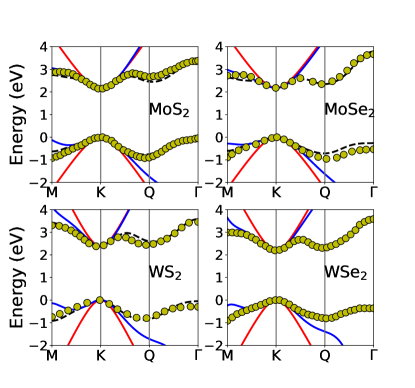
Figure 3: $k\cdot p$ band structure of monolayer TMDs with (blue), and without (red) taking into account the electron-hole asymmetry, TW and nonparabolic effects, compared with the TB calculations (black dashed lines), and DFT results (yellow dots) collected from various references. Rybkovskiy, C.Gerber, and Durnev (2017); Jeong et al. (2018); Zhang et al. (2017); Fang et al. (2018a) To facilitate the comparison, VB maxima are set to zero energy, and the band gaps in each case is corrected to the values in Table 1.

II.5 Spin-dependent four-band $k\cdot p$ Hamiltonian

Due to the presence of heavy metal atoms in TMDs, the spin-orbit interaction is quite strong Pearce, Mariani, and Burkard (2016) in contrast to for instance, monolayer graphene and hBN.Fang et al. (2018a) The spin-dependent effects in TMDs are commonly incorporated within the spin-diagonal and wave vector-independent approximation.Xiao et al. (2012); Liu et al. (2013); Kormányos et al. (2013, 2015) Thus, we first generalize the two-band Hamiltonian of Eq. (3) into a form with spin-dependent diagonal entries as

$$H_{\mathrm{2B}}=\left(\begin{array}[]{cc}h_{11}&h_{12}\\ h^{*}_{12}&h_{22}\end{array}\right)\longrightarrow~{}~{}H^{\downarrow,\uparrow}_{\mathrm{2B}}=\left(\begin{array}[]{cc}h^{\downarrow,\uparrow}_{11}&h_{12}\\ h^{*}_{12}&h^{\downarrow,\uparrow}_{22}\end{array}\right),$$ (19)

by modifying only the electron-hole asymmetry contribution in Eq. (6) so that it becomes

$$H^{\downarrow,\uparrow}_{\mathrm{asym}}=k^{2}\left(\begin{array}[]{cc}\beta^{\downarrow,\uparrow}&0\\ 0&\alpha^{\downarrow,\uparrow}\end{array}\right),$$ (22)

where the fitted $\beta^{\downarrow,\uparrow}$ and $\alpha^{\downarrow,\uparrow}$ to the corresponding effective mass values are tabulated in Table 3. We keep the remaining two-band $k\cdot p$ parameters ($f_{1},f_{2},f_{4},f_{5},\kappa,\eta$) as in Table 2, and in this way we do not inflate the number of fitting parameters significantly.

With these ingredients the two-band formalism is extended into both spin channels that results in the four-band $k\cdot p$ Hamiltonian which is expressed in the Bloch basis ordering of $\left\{\ket{\bm{k},\,d_{z^{2}},\uparrow},\,\ket{\bm{k},\,d_{z^{2}},\downarrow},\,\ket{\bm{k},\,d_{x^{2}-y^{2}}+id_{xy},\uparrow},\,\ket{\bm{k},\,d_{x^{2}-y^{2}}+id_{xy},\downarrow}\right\}$ as

$$H_{\mathrm{4B}}=\left(\begin{array}[]{cccc}h^{\uparrow}_{11}&0&h_{12}&0\\ 0&h^{\downarrow}_{11}&0&h_{12}\\ h^{*}_{12}&0&h^{\uparrow}_{22}&0\\ 0&h^{*}_{12}&0&h^{\downarrow}_{22}\end{array}\right)+\tau\left(\begin{array}[]{cccc}-\Delta^{\mathrm{so}}_{\mathrm{cb}}&0&0&0\\ 0&0&0&0\\ 0&0&-\Delta^{\mathrm{so}}_{\mathrm{vb}}&0\\ 0&0&0&0\end{array}\right),$$ (23)

where $\tau$ is the valley index with value $+1$ ($-1$) for the $+K$ ($-K$) valley, and $\Delta^{\mathrm{so}}_{\mathrm{cb}}$ ($\Delta^{\mathrm{so}}_{\mathrm{vb}}$) is the CB (VB) spin splitting as listed in Table 3.

Table 3: Additional spin-dependent $k\cdot p$ parameters required for the four-band Hamiltonian. CB and VB spin splittings are taken from spin-polarized DFT band structure.Kormányos et al. (2015) $\alpha^{\downarrow}$ and $\beta^{\downarrow}$ values coincide with the two-band values in Table 2.

TMD	MoS2	MoSe2	WS2	WSe2
$\Delta^{\mathrm{so}}_{\mathrm{cb}}$ (meV)	-3	-22	32	37
$\Delta^{\mathrm{so}}_{\mathrm{vb}}$ (meV)	148	186	429	466
$\alpha^{\downarrow}$ (eV$\cdot$Å2)	4.16	5.22	8.2	8.43
$\beta^{\downarrow}$ (eV$\cdot$Å2)	-2.35	-3.9	-4.43	-5.4
$\alpha^{\uparrow}$ (eV$\cdot$Å2)	4.23	5.22	8.58	8.85
$\beta^{\uparrow}$ (eV$\cdot$Å2)	-2.2	-3.86	-5.47	-6.15

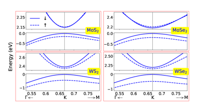
Figure 4: Four-band $k\cdot p$ band structure of monolayer TMDs around the $K$ valley for spin $\downarrow$ (solid) and spin $\uparrow$ (dashed) bands. Abscissae are in units of $2\pi/a$. Spin-dependent parameters are listed in Table 3, and the remaining spin-independent parameters ($f_{1},f_{2},f_{4},f_{5},\kappa,\eta$) are used from Table 2.

Figure 4 shows the spin-dependent band structure of the monolayer TMDs around the $K$ valley. As the spin-dependent parameters in Eq. (23) reside on the diagonal entries, in this level of approximation spin remains to be a good quantum label. Xiao et al. (2012) Another convenience of this approach is that the aforementioned two-band model directly corresponds to the spin-$\downarrow$ sector of the four-band Hamiltonian. Therefore, when lowest-lying spin-allowed transitions (as in the so-called $A$-excitons) are of interest,Wang et al. (2018) the spinless two-band variant in Sec. II.1 can be employed.

III Results and Discussion

To demonstrate several aspects of the geometric band properties we choose monolayer WSe₂ as the prototypical TMD material, and focus on the bands with the narrowest spin-allowed bandgap transition which corresponds to spin–$\downarrow$ sector at the $K$ valley (solid lines in Fig. 4) which essentially reduces the computational task to the two-band $k\cdot p$, and the three-band TB cases, as mentioned above. Starting with the unstrained case in Fig. 5, the top VB and bottom CB behaviors for both of these models are in qualitative agreement around $K$ valley edge, with the variation in the TB being wider for both geometric quantities. The significance of TW on these can be clearly observed together with the fact that BC toggles sign between VB and CB while this is not the case for the OMM.

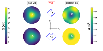
(a)

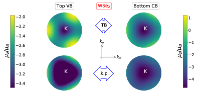
(b)

Figure 5: (a) BC and (b) OMM of (spin $\downarrow$) CB and VB for an unstrained monolayer WSe₂. The part of the Brillouin zone centered at the $K$ point over a radius of $0.12\times 2\pi/a$ is shown, maintaining the same axial orientation as in Fig. 2.

III.1 Effects of strain

Figure 6 shows the effects of strain on the (a) BC, and (b) OMM for the monolayer WSe₂ over the $Q-K-M$ path within the Brillouin zone, where the $Q$ point lies exactly at midway between the $\Gamma$ and $K$ points. First considering the TB results, the geometric properties are seen to be inflated as the strain changes from compressive to tensile nature. However, this simple behavior is localized to the $K$ valley, especially for the VB. In the case of the CB, the variation gets reversed beyond the halfway between the $Q-K$ panel, due to the satellite CB valley at the $Q$ point.Kormányos et al. (2015) Switching to $k\cdot p$ results, in the vicinity of $K$ valley they display a behavior close to TB but again with somewhat reduced amplitudes. The incremental contribution of each term in the Hamiltonian (Eqs. (6)$-$(12)) indicates that the cubic term actually deteriorates the agreement with TB toward the $M$ point by introducing an extra curvature for both VB and CB, yet it was observed in Fig. 3 to have a positive impact on the band structure for the same point.

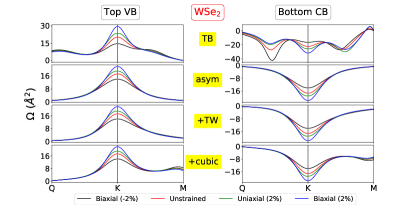
(a)

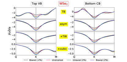
(b)

Figure 6: Effect of strain for a monolayer WSe₂ on (a) BC and (b) OMM of (spin $\downarrow$) CB and VB according to TB (top rows) and $k\cdot p$ (remaining rows) models, where for the latter the effect of each additional term (Eqs. (6)$-$(12)) is shown.

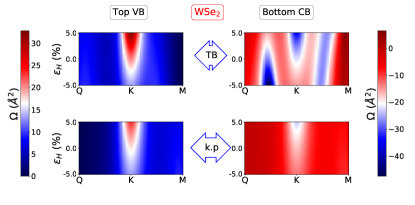
(a)

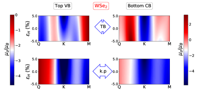
(b)

Figure 7: Effect of (compressive/tensile) hydrostatic strain, $\varepsilon_{H}=\varepsilon_{xx}+\varepsilon_{yy}$ on (a) BC and (b) OMM of (spin $\downarrow$) CB and VB for a monolayer WSe₂.

These traits are more clearly demonstrated in Fig. 7 where the continuous tunability of both BC and OMM under hydrostatic strain $\varepsilon_{H}=\varepsilon_{xx}+\varepsilon_{yy}$ is displayed. Once again, $k\cdot p$ while in qualitative agreement with TB around the $K$ valley, it cannot reproduce the broad variations; particularly for the CB the $Q-K$ panel is not satisfactory. As a matter of fact a separate $k\cdot p$ Hamiltonian needs to be invoked to replicate the correct behavior around the CB $Q$ valley.Kormányos et al. (2015) Apart from these discrepancies at regions with relatively low curvature, both techniques reveal that the $K$ point geometric band properties can be doubled with respect to unstrained values by about +5% hydrostatic strain.

We can offer a simple explanation for these increased geometrical band properties under tensile hydrostatic strain by making use of two-band electron-hole symmetric analytical expressions Xiao, Yao, and Niu (2007); Chen et al. (2019) for the $K$ point: $\Omega_{z}=\pm 2(f_{2}a/E_{g})^{2}$, $\mu_{z}=\mu_{B}m_{0}/m^{*}$, where the strained band gap Aas and Bulutay (2018) $E_{g}=f_{1}+2f_{4}\varepsilon_{H}$, and the strained effective mass Aas and Bulutay (2018) $m^{*}=\pm\hbar^{2}E_{g}/[2(f_{2}a)^{2}]$. Since $f_{4}<0$ (cf. Table 2), a tensile hydrostatic strain $(\varepsilon_{H}>0)$ decreases the $E_{g}$. Hence, this decrease in band gap is the common origin for the improvement in both BC and OMM. As applying a tensile strain to a monolayer TMD is far less problematic than a compressive one which would lead to the buckling of the membrane,Amorim et al. (2016) it warrants a realistic strain enhancement of the geometric band properties.

IV Conclusions

The appealing features of TMDs can be traced down largely to geometric band effects controlled by BC and OMM. Moreover, they can be widely tuned by exerting strain. To harness these in device applications accurate and physically-transparent band structure tools are needed. In this work we offer two options: a $k\cdot p$ model (two- or a four-band) having an up-to-date parameter set, and a strained extension of a three-band TB Hamiltonian. Despite their simplicity, both capture the essential physics that govern the variation of BC and OMM, but with different validity ranges around the $K$ valley. Quantitatively, we report under reasonable biaxial tensile strains (about 2.5%) that these can be doubled in value. It is straightforward to incorporate excitonic effects to this framework. Aas and Bulutay (2018) Thus, these models may serve for TMD device modeling purposes under electric, magnetic or optical excitations in addition to strain.

References

- Xu et al. (2014) X. Xu, W. Yao, D. Xiao, and T. F. Heinz, Nat. Phys. 10, 343–350 (2014).
- Manzeli et al. (2017) S. Manzeli, D. Ovchinnikov, D. Pasquier, O. V. Yazyev, and A. Kis, Nat. Rev. Mater. 2, 17033 (2017).
- Mak, Xiao, and Shan (2018) K. F. Mak, D. Xiao, and J. Shan, Nat. Photon. 12, 451–460 (2018).
- Yamamoto et al. (2015) M. Yamamoto, Y. Shimazaki, I. V. Borzenets, and S. Tarucha, J. Phys. Soc. Jpn. 84, 121006 (2015).
- Schaibley et al. (2016) J. R. Schaibley, H. Yu, G. Clark, P. Rivera, J. S. Ross, K. L. Seyler, W. Yao, and X. Xu, Nat. Rev. Mat. 1, 16055 (2016).
- Xiao, Yao, and Niu (2007) D. Xiao, W. Yao, and Q. Niu, Phys. Rev. Lett. 99, 236809 (2007).
- Yao, Xiao, and Niu (2008) W. Yao, D. Xiao, and Q. Niu, Phys. Rev. B 77, 235406 (2008).
- Xiao et al. (2012) D. Xiao, G. B. Liu, W. Feng, X. Xu, and W. Yao, Phys. Rev. Lett. 108, 196802 (2012).
- Mak et al. (2014) K. F. Mak, K. L. McGill, J. Park, and P. L. McEuen, Science 344, 1489–1492 (2014).
- Wu et al. (2019) Z. Wu, B. T. Zhou, X. Cai, P. Cheung, G.-B. Liu, M. Huang, J. Lin, T. Han, L. An, Y. Wang, S. Xu, G. Long, C. Cheng, K. T. Law, F. Zhang, and N. Wang, Nat. Comm. 10, 611 (2019).
- Cao et al. (2012) T. Cao, G. Wang, W. Han, H. Ye, C. Zhu, J. Shi, Q. Niu, P. Tan, E. Wang, B. Liu, and J. Feng, Nat. Commun. 3, 887 (2012).
- Vanderbilt (2018) D. V. Vanderbilt, Berry Phases in Electronic Structure Theory (Cambridge University Press, Cambridge, 2018).
- Xiao, Chang, and Niu (2007) D. Xiao, M.-C. Chang, and Q. Niu, Rev. Mod. Phys. 82, 1959–2007 (2007).
- Zhang, Shan, and Xiao (2018) X. Zhang, W.-Y. Shan, and D. Xiao, Phys. Rev. Lett. 120, 077401 (2018).
- Cao, Wu, and Louie (2018) T. Cao, M. Wu, and S. G. Louie, Phys. Rev. Lett. 120, 077401 (2018).
- Srivastava and Imamoğlu (2015) A. Srivastava and A. Imamoğlu, Phys. Rev. Lett. 115, 166802 (2015).
- Zhou et al. (2015) J. Zhou, W.-Y. Shan, W. Yao, and D. Xiao, Phys. Rev. Lett. 115, 166803 (2015).
- Chang and Niu (2008) M.-C. Chang and Q. Niu, J. Phys.: Condens. Matter 20, 193202 (2008).
- Brooks and Burkard (2017) M. Brooks and G. Burkard, Phys. Rev. B 95, 245411 (2017).
- Rybkovskiy, C.Gerber, and Durnev (2017) D. V. Rybkovskiy, I. C.Gerber, and M. V. Durnev, Phys. Rev. B 95, 155406 (2017).
- Aivazian et al. (2015) G. Aivazian, Z. Gong, A. M. Jones, R. L. Chu, J. Yan, D. G. Mandrus, C. Zhang, D. Cobden, W. Yao, and X. Xu, Nat. Phys. 11, 148–152 (2015).
- Srivastava et al. (2015) A. Srivastava, M. Sidler, A. V. Allain, D. S. Lembke, A. Kis, and A. Imamoğlu, Nat. Phys. 11, 141–147 (2015).
- Schüler et al. (2019) M. Schüler, U. D. Giovannini, H. Hübener, A. Rubio, M. A. Sentef, and P. Werner, arXiv preprint arXiv:1905.09404 (2019).
- Bertolazzi, Brivio, and Kis (2011) S. Bertolazzi, J. Brivio, and A. Kis, ACS Nano 5, 9703–9709 (2011).
- Kormányos et al. (2015) A. Kormányos, G. Burkard, M. Gmitra, J. Fabian, V. Zólyomi, N. D. Drummond, and V. I. Fal’ko, 2D Materials 2, 022001 (2015).
- Rostami et al. (2015) H. Rostami, R. Roldán, E. Cappelluti, R. Asgari, and F. Guinea, Phys. Rev. B 92, 195402 (2015).
- Pearce, Mariani, and Burkard (2016) A. J. Pearce, E. Mariani, and G. Burkard, Phys. Rev. B 94, 155416 (2016).
- Sevik et al. (2017) C. Sevik, J. R. Wallbank, O. Gülseren, F. M. Peeters, and D. Çakır, 2D Mater. 4, 035025 (2017).
- Fang et al. (2018a) S. Fang, S. Carr, M. A. Cazalilla, and E. Kaxiras, Phys. Rev. B 98, 075106 (2018a).
- Aas and Bulutay (2018) S. Aas and C. Bulutay, Opt. Express 26, 28672–28681 (2018).
- Zhang et al. (2014) Y. J. Zhang, T. Oka, R. Suzuki, J. T. Ye, and Y. Iwasa, Science 344, 725–728 (2014).
- Li et al. (2014) Y. Li, J. Ludwig, T. Low, A. Chernikov, X. Cui, G. Arefe, Y. D. Kim, A. M. van der Zande, A. Rigosi, H. M. Hill, S. H. Kim, J. Hone, Z. Li, D. Smirnov, and T. F. Heinz, Phys. Rev. Lett. 113, 266804 (2014).
- MacNeill et al. (2015) D. MacNeill, C. Heikes, K. F. Mak, Z. Anderson, A. Kormányos, V. Zólyomi, J. Park, and D. C. Ralph, Phys. Rev. Lett. 114, 037401 (2015).
- Kormányos et al. (2013) A. Kormányos, V. Zólyomi, N. D. Drummond, P. Rakyta, G. Burkard, and V. I. Fal’ko, Phys. Rev. B 88, 045416 (2013).
- Chen et al. (2019) S.-Y. Chen, Z. Lu, T. Goldstein, J. Tong, A. Chaves, J. Kunstmann, L. S. R. Cavalcante, T. Woźniak, G. Seifert, D. R. Reichman, T. Taniguchi, K. Watanabe, D. Smirnov, and J. Yan, Nano Lett. 19, 2464–2471 (2019).
- Bromley, Murray, and Yoffe (1972) R. A. Bromley, R. B. Murray, and A. D. Yoffe, J. Phys. C: Solid State Phys. 5, 759–778 (1972).
- Cappelluti et al. (2013) E. Cappelluti, R. Roldán, A. Silva-Guillén, P. Ordejón, and F. Guinea, Phys. Rev. B 88, 075409 (2013).
- Liu et al. (2013) G. B. Liu, W. Y. Shan, Y. Yao, W. Yao, and D. Xiao, Phys. Rev. B 88, 085433 (2013).
- Fang et al. (2018b) S. Fang, R. K. Defo, S. N. Shirodkar, S. Lieu, G. A. Tritsaris, and E. Kaxiras, Phys. Rev. B 92, 205108 (2018b).
- Jeong et al. (2018) J. Jeong, Y. H. Choi, K. Jeong, H. Park, D. Kim, and M. H. Cho, Phys. Rev. B 97, 075433 (2018).
- Zhang et al. (2017) L. Zhang, Y. Huang, Q. Zhao, L. Zhu, Z. Yao, Y. Zhou, W. Du, and X. Xu, Phys. Rev. B 96, 155202 (2017).
- Rasmussen and Thygesen (2015) F. A. Rasmussen and K. S. Thygesen, J. Phys. Chem. C 119, 13169–83 (2015).
- Thygesen (2017) K. S. Thygesen, 2D Mater. 4, 022004 (2017).
- Feng et al. (2012) W. Feng, Y. Yao, W. Zhu, J. Zhou, W. Yao, and D. Xiao, Phys. Rev. B 86, 165108 (2012).
- Wang et al. (2018) G. Wang, A. Chernikov, M. M. Glazov, T. F. Heinz, X. Marie, T. Amand, and B. Urbaszek, Rev. Mod. Phys. 90, 021001 (2018).
- Amorim et al. (2016) B. Amorim, A. Cortijo, F. de Juan, A. Grushin, F. Guinea, A. Gutiérrez-Rubio, H. Ochoa, V. Parente, R. Roldán, P. San-Jose, J. Schiefele, M. Sturla, and M. Vozmediano, Phys. Rep. 617, 1 – 54 (2016).