Anomaly Detection with
HMM Gauge Likelihood Analysis

Abstract

This paper describes a new method, HMM gauge likelihood analysis, or GLA, of detecting anomalies in discrete time series using Hidden Markov Models and clustering. At the center of the method lies the comparison of subsequences. To achieve this, they first get assigned to their Hidden Markov Models using the Baum-Welch algorithm. Next, those models are described by an approximating representation of the probability distributions they define. Finally, this representation is then analyzed with the help of some clustering technique or other outlier detection tool and anomalies are detected. Clearly, HMMs could be substituted by some other appropriate model, e.g. some other dynamic Bayesian network. Our learning algorithm is unsupervised, so it doesn’t require the labeling of large amounts of data. The usability of this method is demonstrated by applying it to synthetic and real-world syslog data.

I Introduction

The detection of anomalies in data is currently one of the most important practical applications of unsupervised learning. It helps companies to understand their data better, to find hidden flaws in complex systems, and to react early to the emergence of unexpected situations. The assumption here is that anything that is anomalous is potentially indicating some kind of failure, malicious behavior, or otherwise exceptional incident that needs attending to. While anomalous patterns can occur in all kinds of data, in this paper we are exclusively dealing with anomaly detection in time series. One important example of time series data in a complex system would be the logging data in a computer network. Today the computer networks of large companies can easily consist of several thousands of machines, each one running a wide range of applications that often use the logging framework syslogd to log their status and important events. This is, of course, a valuable source for diagnostics and predictive maintenance.

The thorough analysis of large amounts of data is usually hampered by mainly two problems: first, the amount of data is often too huge for humans to read through, and second, the experts which can interpret the data are usually very hard to find. Thus, it would be very helpful, if this analysis could be automated, at least partially. One approach often used is that of anomaly detection: use machine learning to learn models that describe the normal behavior and then label those patterns, that cannot be described well by the learned models, as anomalous. The advantages of anomaly detection are that large amounts of data can be processed automatically and that no experts are necessary. Moreover, anomaly detection algorithms can often detect strange patterns in data that look innoxious even to an expert. Also, the algorithms used in this paper are unsupervised, i.e. they don’t need labeled data for learning, which for large data is in general very difficult to obtain. The disadvantage is, that it is often difficult to determine the threshold of how anomalous an event has to be for being noted as an anomaly, and that depending on this threshold, we might obtain too many false positives or too many false negatives. And, of course, there is always the possibility of rare but harmless events, as well as critical events that have a high frequency; anomaly detection cannot help in those situations and other methods have to be applied.

There are many different types of anomalies possible, as there are many different types of patterns that data can contain, and violations of those patterns can be considered anomalies. One very simple pattern in time series data that could be exploited is the simple presence of certain events. And if some events are usually not present, i.e. have a low frequency, their occurrence would then be considered an anomaly. Thus, one conceptually very easy anomaly detection method is the frequency analysis of events. We specify a threshold for the frequency, and any event frequency below this threshold is considered an anomaly and this rare event should be examined more closely. The threshold itself depends on the given situation and should be adapted accordingly. So in this case, the “machine learning” part simply consists in recording the frequencies of events and then applying a threshold.

Other patterns, that could be used for time series anomaly detection are the ratios, or more general linear dependencies of event counts, for example within a certain time window. That means, contrary to the example above, here we don’t just consider individual events but rather aggregations of events. One way of implementing this is by using PCA on event counts [Xu et al., 2010a].

Yet another type of pattern is the consecution of events. Thus, while the pattern in this case also consists of aggregations of events as the ratio pattern above, now also the order of events is relevant. So, for example, if our event time series consists of two events in the form (A, B, A, B, A, B, …) and then suddenly there would appear the sequence (A, A, A, B, B, B), the ratio anomaly detection would not be triggered, but the order anomaly detection would. This variant has been investigated in many papers, and it is also the focus of the current paper.

The method that is described in this paper could be delineated shortly as follows: We consider one long time series of events and cut it into a series of smaller sequences that are all of the same length, e.g. 20 events long. To describe them properly, we map them to their Hidden Markov Models (HMM). Two sequences are then considered similar if their HMMs are similar. Since HMMs are non-identifiable, comparing them is nontrivial. We consider them as probability distributions over the space of event sequences. So we take a few, e.g. 10, fixed event sequences and compute their probabilities wrt. the HMMs, creating a vector of probabilities for each HMM. If those vectors are similar for two HMMs, it is likely that the HMMs have similar probability distributions and thus are similar themselves. This, in turn, means, that their original event sequences are similar. Thus, we have a nontrivial feature engineering scheme, that maps sequences to vectors of probabilities that can then be searched for outliers, e.g. by clustering algorithms that detect outliers like for instance HDBSCAN or simply by visually inspecting the two-dimensional t-SNE projection.

We demonstrate this method with synthetic data as well as real-world syslog data.

II RELATED WORK

Here we give a very short and rather incomplete review of the literature on anomaly detection for time series data with a finite value space. For a more comprehensive overview, see e.g. [Chandola et al., 2012].

The approach most often used in anomaly detection with machine learning is to learn a model from the normal patterns and then to declare all patterns, to which the model assigns very low probability, to be anomalous.

Some authors partition the time into intervals and consider histograms of the frequencies of the events in each window, which results in a collection of histograms. Since the value (event) space is finite, those histograms are points in a finite-dimensional vector space. This collection of points can now be approximated with PCA and points very far away from the PCA subspace will be labeled anomalous. This idea is exploited for example in [Xu et al., 2010a], [Xu et al., 2009], and [Xu et al., 2010b]. In those papers, neither the sequential ordering inside the windows nor the order of the windows themselves is used, only the linear relations of the frequencies of nearby events are taken into account.

If we want to include the order of events in our analysis, we enter the realm of time series analysis. One very powerful tool in time series analysis are Hidden Markov Models (HMMs) and so it is not surprising that they have been used a lot for this kind of anomaly detection. There are many different variants in which HMMs can enter the scene. The most popular approach is to compute an HMM for the normal data and then compute for all new data sequences their probabilities wrt. this HMM. If the probability of the sequence is too small, i.e. is below a carefully chosen threshold, the sequence is labeled as anomalous. This method can be found for example in [Chandola et al., 2012], [Lane and Brodley, 2003], [Joshi and Phoha, 2005], [Khreich et al., 2009], [Khreich et al., 2010], [Lane and Brodley, 2003] or [Wang et al., 2004]. A similar idea can be found in [Dorj et al., 2013], which replaces HMMs with Bayesian HMMs. The problem with all those techniques is that they are not very good in modeling multiple types of sequences. They work best if there is just one main sequential structure present in the normal data. However, we are interested in situations of long sequences that can display several different patterns and it turned out that this method does not give usable results.

HMMs are often interpreted as finding, to the given observed sequence, an underlying sequence of “hidden” states, which are thought of as causing the observations. Often, the HMM is chosen to have fewer values in the hidden states than in the observations, which makes the hidden sequence less complex and easier to compute with. One interpretation could be that the observations are the states with added noise. This point of view leads to the idea of replacing the observed sequence with the sequence of hidden states and then doing anomaly detection on this one (for example by comparing them to a database of labeled sequences, using an appropriate similarity measure). For work along this line of reasoning, see e.g. [Chandola et al., 2012] or [Chandola et al., 2008], and references therein. However, this method, too, suffers from the drawbacks described before and is not usable for our purposes.

One problem with HMMs is that with longer sequences with many states, computations become slow and sometimes lead to arithmetic underflow. In [Florez-Larrahondo et al., 2005] they developed an iterative version of HMMs that alleviates those problems.

Another problem is the choice of the number of hidden states. Most often, this parameter is simply tuned according to what works best in the given situation. A more principled approach is taken by [Khreich et al., 2009], which choose a combination of HMMs with different state counts by using the “Maximum Realizable ROC” technique. Then again, the anomalies are detected via a carefully chosen probability threshold. An extension of this scheme can be found in [Khreich et al., 2010]. One further approach to anomaly detection that uses combinations of HMMs is demonstrated in [Yamanishi and Maruyama, 2005] which uses mixtures of HMMs. The machinery described is quite complex. However, the clustering described there did not work well with our data. We think that is due to two problems: first, the number of components needs to be provided to the algorithm and the dynamic selection of this number described in the paper was not very robust. Second, the range of possible shapes of clusters is bounded and cannot be as arbitrary as with e.g. HDBSCAN.

Of course, today, with the rise of deep learning [Goodfellow et al., 2016] in almost all fields of machine learning, there are also applications of this new paradigm to anomaly detection. Some work has been published in this area in the last few years, but we will not go into detail here and only mention two general approaches. One considers anomaly detection simply as a classification problem (i.e. is only applicable to labeled data), and can thus apply one of the standard deep neural network architectures for supervised learning. E.g. in [Javaid et al., 2016], they train a deep sparse autoencoder network. Another approach does anomaly detection via time series prediction. It learns Recurrent Neural Networks (RNNs) [Sutskever, 2013] for the event sequences, computes the probability distribution over all possible extrapolations for the next few steps and labels sequences that have low probability with respect to this distribution as anomalous. Quite a number of papers follow this scheme, see e.g. [Malhotra et al., 2015], [Chauhan and Vig, 2015], or [Shipmon et al., 2017], to name only three. A clear advantage of Recurrent Neural Networks, especially Long Short Term Memory (LSTM) models, see [Hochreiter and Schmidhuber, 1997], is that they can much better remember past events than HMMs can. One clear disadvantage of deep neural networks is the often large amount of effort necessary to get the network to converge to a good model. Since anomaly detection via prediction can be done with any prediction method, classical or deep learning, it might be interesting for us to compare the prediction performance of all kinds of prediction models. This has been done several times, for recent results see e.g. [Makridakis et al., 2018b], the NN3 competition [Crone et al., 2005], and the M4 competition [Makridakis et al., 2018a]. In general, deep learning seems like a promising direction for anomaly detection in time series, especially if long term correlations between events are present.

III HMM gauge likelihood analysis

We are concerned with the problem of finding anomalies in discrete time series. In this paper, we consider only batch processing: first, the time series data is collected, let’s say for one whole day, and then this complete batch of data is processed together. The scenario is that of a long time series, i.e. a continuous stream of discrete data, that most of the time behaves normal but at rare occasions digresses from that normal pattern of behavior. Our task is to find those anomalies since they are likely to be of importance e.g. for predictive maintenance. One example would be the syslog events written by a given application. As long as the application always logs the same sequences of events, everything is fine. However, if this pattern suddenly changes, we would like to know about this change.

The first point to make is that we will not consider the complete time series $T$ as a whole, but rather subsequences $t_{k}$ thereof. To be more precise: for $i,j\in\mathds{N},i\leq j$, let the index set $\bm{I}_{i:j}$ be the set of integers $\{i,i+1,\ldots,j\}$. Moreover, let $\mathfrak{E}$ be the set of possible events we can observe. Then we consider all the subsequences $t^{n}_{k}$ of length $n$ of the total sequence $T$ of length $N$ that are obtained by sliding a window of size $n$ with a step size $m$ over the domain of $T$, i.e.:

$$\begin{split}&T:\bm{I}_{1:N}\to\mathfrak{E}\\ &t^{n}_{k}:\bm{I}_{1:n}\to\mathfrak{E},\;n\in\mathds{N},\;n\leq N,\quad k=1,2,\ldots,\lfloor(N+m-n)/m\rfloor\\ &t^{n}_{k}(l):=T(l+(k-1)m),\quad l\in\bm{I}_{1:n},\end{split}$$ (1)

where we often omit the superscript $n$. Note that at the end of $T$ we don’t keep windows that are incomplete (in case $N-n$ is not dividable by $m$). The window size $n$ should be a small multiple of the expected maximal autocorrelation distance, so the model has a chance to learn those correlations. As the window shift size $m$ we usually choose half the window size: $n/2$.

It is those subsequences $t_{k}$ that we want to compare. Usually, most are similar to each other and some are different and the latter are the anomalies. The common length $n$ of those subsequences should not be too small, such that they will still contain a sufficient amount of most of the behavioral patterns. On the other hand, because of computational constraints like arithmetic underflow and computation time, the length cannot be too large. Thus, this parameter has to be tuned according to the situation at hand.

Our next step is to find a way to compare the subsequences $t_{k},k=1,\ldots,K$. Unfortunately, comparing sequences to each other is not trivial. We could, for example, compare two sequences $t_{r}=(t_{ri})_{i=1}^{n}$ and $t_{s}=(t_{si})_{i=1}^{n}$ by taking the Euclidean distance between those two vectors: $d_{E}(t_{r},t_{s})=\sqrt{\sum_{i=1}^{n}|t_{ri}-t_{si}|^{2}}$. But this measure has several flaws. For example, this would mean that two sequences that just differ by a simple time shift could be considered completely different. There are several possible approaches to measuring the similarity of sequences that avoid this and similar problems. Our choice in this paper is to compare two sequences by comparing the HMMs that have been learned from them using the Baum-Welch algorithm. HMMs are an appropriate model in this situation since they are simple enough to be tractable, yet sufficiently versatile to capture the idiosyncrasies of the sequences they have been fitted to. This has been shown by numerous applications of this popular model. E.g., they are, contrary to ordinary Markov chains, capable of detecting longer lasting autocorrelations. For a good introduction to HMMs, see e.g. [Rabiner, 1989], [Bishop, 2006], or [Prince, 2012].

To assign a HMM model to each sequence $t_{k}$, we have to choose a number of hidden states. Again, this needs to be tuned for the given problem. The trade off here is similar to that for the length of the sequence: large numbers of hidden states on the one hand provide more powerful models, which for example can remember further back in the past, but on the other hand lead to high computational costs.

Unfortunately, HMMs cannot be compared just by comparing the model parameters. Indeed, it is well known that HMMs are non-identifiable, i.e. there are different sets of model parameters that define equivalent models. To understand this, first note that statistical models such as HMMs assign a probability to each possible data input, in our case to each possible sequence of the same length $n$ as the HMM. More formally: Let $n$ be the chosen length of the event sequences. Also, recall that $\bm{I}_{n}$ is the index set containing the first $n$ natural numbers $\bm{I}_{n}:=\{1,\ldots,n\}$, and that $\mathfrak{E}$ is the set of all possible events that can happen. Then:

$$\mathcal{S}_{n}=\{s|s:\bm{I}_{n}\to\mathfrak{E}\}$$ (2)

is the set of all possible event sequences of length $n$ with event space $\mathfrak{E}$. Of course, our original subsequences $t_{k}$ are also contained in this set: $t_{k}\in\mathcal{S}_{n},k=1,\ldots,K$. Further, let $\theta$ be the vector containing all the parameters of an HMM, and let $h(\theta)$ be the belonging HMM. Then each HMM $h(\theta)$ of length $n$ defines a probability distribution function (PDF) $p_{h(\theta)}$ over $\mathcal{S}_{n}$:

$$p_{h(\theta)}:\mathcal{S}_{n}\to[0,1],\quad\sum_{s\in\mathcal{S}_{n}}p_{h(\theta)}(s)=1.$$ (3)

Now, for any practical purposes, two HMMs $h(\theta_{1})$ and $h(\theta_{2})$ are indistinguishable if they define the same PDF over $\mathcal{S}_{n}$:

$$h(\theta_{1})=h(\theta_{2})\quad\coloneqq\quad\forall_{s\in\mathcal{S}}\;\;p_{h(\theta_{1})}(s)=p_{h(\theta_{2})}(s).$$ (4)

Indeed, they should be considered equal, since there is no experiment that can prove them different. In general, models with the property that different model parameters $\theta_{1}$ and $\theta_{2}$ can lead to the same probability distribution are called non-identifiable. Now, as mentioned above, HMMs happen to have this property, i.e., with the above notation:

$$\exists_{\theta_{1},\theta_{2},\theta_{1}\neq\theta_{2}}\quad h(\theta_{1})=h(\theta_{2}).$$ (5)

One very simple example is that we can single out two states and then switch in the transition matrix the belonging two rows and columns, and in the emission matrix the two rows belonging to the two states. This will not change the probability distribution but the parameters will in general change. This can, of course, be done with any arbitrary permutation of states. Note, however, that there are many more ways in which identifiability is violated in HMMs, not just via permutations. For more background on non-identifiability of HMMs and its algebraic geometrical structure see e.g. [Watanabe, 2001] and [Hosino et al., 2005]. The important implication for our purposes is that the parameters of HMMs cannot be used to compare them since models that are similar or equivalent can have very different sets of parameters.

The above explanation takes the approach of viewing statistical models, and in our case HMMs in particular, as probability distributions over the data. And this view is also what leads us to the feature map that we choose in our approach. Ideally, we would take as features the probability distributions $p_{h}(\theta)$ themselves. But, of course, comparing probability distributions is not realistic because of the large size of $\mathcal{S}_{n}$ even for moderately sized $n$ and $\mathfrak{E}$. Thus, instead of comparing the probabilities of each and every single sequence $s\in\mathcal{S}_{n}$, only a small number $m$ of them is selected. Those chosen sequences then define a map $\ell$ from the set of HMM models $\mathcal{H}$ to $\mathds{R}^{m}$. More formally: Let $\mathcal{G}$ be the set of sequences chosen to compare HMMs:

$$\mathcal{G}=\{g_{1},\ldots,g_{m}\},\quad g_{i}\in\mathcal{S}_{n},\;i=1,\ldots,m.$$ (6)

Then the map $\ell$ is defined as follows:

$$\begin{split}&\ell:\mathcal{H}\to\mathds{R}^{m},\\ &\ell(h):=(p_{h}(g_{1}),\ldots,p_{h}(g_{m}))\in\mathds{R}^{m}.\end{split}$$ (7)

The sequences $g_{i}\in\mathcal{G}$ are the basis for comparing the HMMs, i.e. they gauge our comparisons. Because of this, we will refer to those sequences as gauge sequences.

Thus, for the comparison of two models $h(\theta_{1})$ and $h(\theta_{2})$, we don’t use their parameters $\theta_{1}$ and $\theta_{2}$ but rather their images under $\ell$ in $\mathds{R}^{m}$. As far as the choice of gauge sequences is concerned, we investigated two approaches. One was choosing a couple of sequences at random. The number of random gauge sequences was not very important as long as it was not below five. The other approach was to use the original sequences themselves. In our experiments, the latter approach showed slightly better cluster separation properties, while requiring more computation time.

To summarize, instead of comparing the sequences directly, we use a feature map that assigns each sequence to a point in an $m$-dimensional cube $[0,1]^{m}$ where $m$ is the number of gauge sequences, and then analyze those image points instead. To detect outliers in this feature space we first apply t-SNE [Maaten and Hinton, 2008] to map the points into $\mathds{R}^{2}$ and then use HDBSCAN [Campello et al., 2013]. It has turned out that using t-SNE before clustering gives superior results. Moreover, the projection to a two-dimensional space allows for easy visualization.

We refer to this method of outlier analysis as HMM gauge likelihood analysis, or GLA for short.

IV Application to synthetic and real data

We evaluated the method on synthetic data as well as real-world data. The results on real-world data were compared with those of a popular deep learning anomaly detection method.

Synthetic data

We have created 60 sequences of length 20, each consisting of the subsequence (A, B, C, D), concatenated five times with small noise added by randomly selecting two elements from each sequence that were altered randomly. Next, we added two anomalous sequences, one which had the order of events reversed, i.e. the sequence was now a repetition of (D, C, B, A), and a second one which was simply a constant sequence, i.e. just 20 times the element A.

Then GLA was applied to this data, using 10 hidden states for the HMMs and ten gauge sequences. The points in the feature space were then projected into $\mathds{R}^{2}$ using t-SNE, see Figure 1. The two outliers are clearly visible near the left edge and the left lower edge of the plot.

Figure 1: A 2D t-SNE plot of simulated data: 60 normal sequences in the upper right corner and two anomalous ones on the left and bottom left.

Another experiment with simulated data is to test the capability of HMMs to remember further back in time than just the previous event, i.e. that they are more powerful than just Markov Chains. For this, we created 500 copies of the sequence $t_{1}$ and one single copy of sequence $t_{2}$:

$$\begin{split}t_{1}=&\mbox{(A, A, B, B, \ \ A, A, B, B, \ \ A, A, B, B,}\\ &\mbox{A, A, B, B, \ \ A, A, B, B, \ \ A)}\\ t_{2}=&\mbox{(A, A, A, A, A, A, \ \ B, B, B, B, B, B,}\\ &\mbox{A, B, A, B, A, B, A, B, A).}\\ \end{split}$$ (8)

Learning a Markov chain on either of those two series would result in the same transition matrix, namely the matrix with all entries equal to 0.5. So a Markov chain model would not be capable to distinguish between those two time series. However, both sequences have clearly different structure which should be detectable for models with memory at least two steps back in the past. The HMM models were configured with four states to be able to remember two steps back. See Figure 2 for the result.

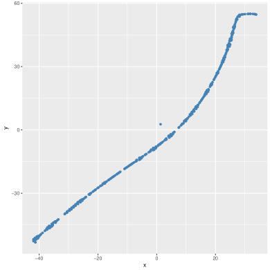
Figure 2: A 2D t-SNE plot of simulated data: 500 normal sequences in the long snake-shaped cluster and one anomalous one near the middle is clearly separated.

The image of the anomalous sequence is clearly visible as an outlier near the middle of the figure.

Real data

Since there is no standard benchmark data for anomaly detection, especially not for syslog data, we used as real data syslog files collected from a Linux laptop and examined those for anomalies. First, some preprocessing was done. There are lots of syslog events that are of the same type and differ only in some details like an IP address or a URL. Most of the time, those details are not relevant and one would like to reduce all those variants into just one single “event type”. For example, a server might get connection requests from thousands of clients and the belonging syslog events would only differ in the URLs of the clients. We would like all those connection requests to be always the same event type, just repeatedly logged.

One could understand this like a clustering of events where we are only interested in the cluster id, which would then be the event type. This clustering in itself is already a nontrivial task and there are several ways to approach this problem, see for example [Vaarandi, 2003] and [Vaarandi and Pihelgas, 2015].

We used a simpler method: from each syslog line, the first three words of the description field that are each at least three characters long and don’t contain any numbers or special characters are extracted as features. The intuition behind this is that the irrelevant details usually show up more towards the end of the log entry and there are rarely two events which coincide in the first three non-numeric words and yet belong to different event types. Verification on the data confirmed that this was a reasonable technique. Below, this will be referred to as the “three first words” feature.

To evaluate GLA, we applied it to the syslog events of several applications. Since our data was not labeled, we had to go through the sequences ourselves and label the anomalies before evaluating our results.

The first example we will discuss here is for the application dhclient. The data contains 46,757 dhclient events, each being one of 9 different event types in the three first words feature. From this sequence, we extracted subsequences over sliding windows of length 20 with shift distance 10. In our manual inspection, we labeled 71 sequences as outliers which were due to rare individual events they contained (we call those “frequential anomalies”). But we did not find any sequence that contained common events in a singular order (we call those “sequential anomalies”).

On each of those dhclient subsequences, we trained an HMM with 20 hidden states. The clustered t-SNE plot of GLA is shown in Figure 3. The clustering resulted in 51 outliers, all of them belonging to the 71 labeled outliers.

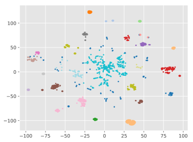
Figure 3: This shows the t-SNE plot of GLA for the application dhclient (sliding window size: 20, shift 10, possible symbols: 9, hidden states: 20), clustered with HDBSCAN. The minimum cluster size parameter of HDBSCAN was set to 20. There are 51 outliers.

The next example we discuss is for the application nm-dispatcher: the data contained 25,352 such events, and again subsequences were extracted with a sliding window of size 20 and a shift distance of 10. The three first words feature for this application gives 16 different event types. Manual labeling let to 34 outliers, consisting of 3 sequential and 31 frequential anomalies. Here, we trained HMMs with 32 hidden states. See Figure 4 for the belonging plot.

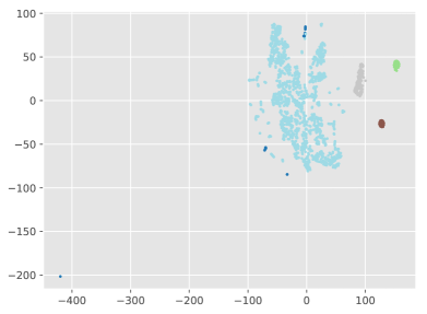
Figure 4: This shows the t-SNE plot of GLA for the application nm-dispatcher (sliding window size: 20, shift 10, possible symbols: 16, hidden states: 32), clustered with HDBSCAN. The minimum cluster size parameter of HDBSCAN was set to 20. There are 7 outliers.

GLA detected seven outliers, one from the sequential outliers, five from the frequential outliers, and one unlabeled one. As usual, the very far outliers, like the one here in the lower left corner, are frequential outliers.

Finally, we investigate the whoopsie application with one sequential outlier and six frequential outliers. See Figure 5 for the visualization of GLA.

Figure 5: This shows the t-SNE plot of GLA for the application whoopsie (sliding window size: 20, shift 10, possible symbols: 15, hidden states: 32), clustered with HDBSCAN. The minimum cluster size parameter of HDBSCAN was set to 20. There are 2 outliers.

Two anomalies where detected. The outlier at the lower right is a frequential outlier, while the one at the middle right is the sequential outlier.

The first five lines of the following table summarize the results.

	dhclient	nm-disp	whoopsie
false pos.	0	1	0
false neg.	20	28	5
recall	$\frac{51}{71}=0.72$	$\frac{6}{34}=0.18$	$\frac{2}{7}=0.28$
precision	$\frac{51}{51}=1$	$\frac{6}{7}=0.86$	$\frac{2}{2}=1$
GLA: F1	$0.84$	$0.30$	$0.44$
LSTM: F1	$0.78$	$0.31$	$0.40$

Obviously, those numbers heavily depend on our choice of the minimum cluster size of HDBSCAN. We preferred choices with less false positives. The parameter was tuned for each application separately.

We compared those results with a popular deep learning anomaly detection method, see [Malhotra et al., 2015]. As discussed above, it uses LSTMs to compute prediction probabilities and if those probabilities, evaluated for the actual sequence, are smaller than a certain threshold, it is considered an anomaly. We used an LSTM of length 20 with 256 units per cell, stacked four times. This model was applied to the three event sequences described above. For comparison with the results for GLA, the threshold for the prediction probabilities was chosen to maximize the F1 score while producing the same number of false positives as GLA. The F1 scores of LSTM have been entered into the last row of the above table. We see that our GLA method outperforms the LSTM model in the first and third case, while in the second case the results are almost identical.

V Conclusions

We have introduced GLA, a new method to detect anomalies in time series data. It computes the HMMs for subsequences and then compares those HMMs with each other by comparing their probability distributions. This is done by computing the probabilities of those HMMs on a vector of gauge sequences and then detecting outliers in the t-SNE projection using appropriate clustering algorithms. The method has been successfully tested with Linux syslog data. The experiments show that the method detects not only rare event anomalies but also sequential anomalies.

VI Future work

In this paper, we have just described the first version of our method, the proof of concept. There are several ways to improve on the current version. The algorithm has still many parameters that need to be chosen, like the size of the subsequences, the number of gauge sequences, the size of the gauge sequences, the number of states of the HMMs, the outlier detection method, and the belonging parameters of this method, such as the minimum cluster size in the case of HDBSCAN. One should investigate to which extend the choice of those parameters can be automated, maybe even learned.

Furthermore, it would be beneficial to see whether other projection methods besides t-SNE, for example UMAP, could improve speed and outlier separation. This should be investigated in tandem with a search for an optimal clustering algorithm for this task.

A very interesting research topic would also be to compare different dynamic Bayesian networks besides HMMs for capturing the sequential patterns in a given population of time series.

References

- [Bishop, 2006] Bishop, C. M. (2006). Pattern Recognition and Machine Learning. Springer.
- [Campello et al., 2013] Campello, R. J., Moulavi, D., and Sander, J. (2013). Density-based clustering based on hierarchical density estimates. In Pacific-Asia conference on knowledge discovery and data mining, pages 160–172. Springer.
- [Chandola et al., 2012] Chandola, V., Banerjee, A., and Kumar, V. (2012). Anomaly detection for discrete sequences: A survey. IEEE Transactions on Knowledge and Data Engineering, 24(5):823–839.
- [Chandola et al., 2008] Chandola, V., Mithal, V., and Kumar, V. (2008). Comparative evaluation of anomaly detection techniques for sequence data. In Data Mining, 2008. ICDM’08. Eighth IEEE International Conference on, pages 743–748. IEEE.
- [Chauhan and Vig, 2015] Chauhan, S. and Vig, L. (2015). Anomaly detection in ecg time signals via deep long short-term memory networks. In Data Science and Advanced Analytics (DSAA), 2015. 36678 2015. IEEE International Conference on, pages 1–7. IEEE.
- [Crone et al., 2005] Crone, S. F., Nikolopoulos, K., and Hibon, M. (2005). Automatic modelling and forecasting with artificial neural networks–a forecasting competition evaluation. Final report for the IIF/SAS Grant, 6:2008.
- [Dorj et al., 2013] Dorj, E., Chen, C., and Pecht, M. (2013). A bayesian hidden markov model-based approach for anomaly detection in electronic systems. In Aerospace Conference, 2013 IEEE, pages 1–10. IEEE.
- [Florez-Larrahondo et al., 2005] Florez-Larrahondo, G., Bridges, S. M., and Vaughn, R. (2005). Efficient modeling of discrete events for anomaly detection using hidden markov models. In International Conference on Information Security, pages 506–514. Springer.
- [Goodfellow et al., 2016] Goodfellow, I., Bengio, Y., Courville, A., and Bengio, Y. (2016). Deep learning, volume 1. MIT press Cambridge.
- [Hochreiter and Schmidhuber, 1997] Hochreiter, S. and Schmidhuber, J. (1997). Long short-term memory. Neural computation, 9(8):1735–1780.
- [Hosino et al., 2005] Hosino, T., Watanabe, K., and Watanabe, S. (2005). Stochastic complexity of variational bayesian hidden markov models. In Neural Networks, 2005. IJCNN’05. Proceedings. 2005 IEEE International Joint Conference on, volume 2, pages 1114–1119. IEEE.
- [Javaid et al., 2016] Javaid, A., Niyaz, Q., Sun, W., and Alam, M. (2016). A deep learning approach for network intrusion detection system. In Proceedings of the 9th EAI International Conference on Bio-inspired Information and Communications Technologies (formerly BIONETICS), pages 21–26. ICST (Institute for Computer Sciences, Social-Informatics and Telecommunications Engineering).
- [Joshi and Phoha, 2005] Joshi, S. S. and Phoha, V. V. (2005). Investigating hidden markov models capabilities in anomaly detection. In Proceedings of the 43rd annual Southeast regional conference-Volume 1, pages 98–103. ACM.
- [Khreich et al., 2010] Khreich, W., Granger, E., Miri, A., and Sabourin, R. (2010). Iterative boolean combination of classifiers in the roc space: An application to anomaly detection with hmms. Pattern Recognition, 43(8):2732–2752.
- [Khreich et al., 2009] Khreich, W., Granger, E., Sabourin, R., and Miri, A. (2009). Combining hidden markov models for improved anomaly detection. In Communications, 2009. ICC’09. IEEE International Conference on, pages 1–6. IEEE.
- [Lane and Brodley, 2003] Lane, T. and Brodley, C. E. (2003). An empirical study of two approaches to sequence learning for anomaly detection. Machine learning, 51(1):73–107.
- [Maaten and Hinton, 2008] Maaten, L. v. d. and Hinton, G. (2008). Visualizing data using t-sne. Journal of machine learning research, 9(Nov):2579–2605.
- [Makridakis et al., 2018a] Makridakis, S., Spiliotis, E., and Assimakopoulos, V. (2018a). The m4 competition: Results, findings, conclusion and way forward. International Journal of Forecasting.
- [Makridakis et al., 2018b] Makridakis, S., Spiliotis, E., and Assimakopoulos, V. (2018b). Statistical and machine learning forecasting methods: Concerns and ways forward. PloS one, 13(3):e0194889.
- [Malhotra et al., 2015] Malhotra, P., Vig, L., Shroff, G., and Agarwal, P. (2015). Long short term memory networks for anomaly detection in time series. In Proceedings, page 89. Presses universitaires de Louvain.
- [Prince, 2012] Prince, S. J. (2012). Computer vision: models, learning, and inference. Cambridge University Press.
- [Rabiner, 1989] Rabiner, L. R. (1989). A tutorial on hidden markov models and selected applications in speech recognition. Proceedings of the IEEE, 77(2):257–286.
- [Shipmon et al., 2017] Shipmon, D. T., Gurevitch, J. M., Piselli, P. M., and Edwards, S. T. (2017). Time series anomaly detection; detection of anomalous drops with limited features and sparse examples in noisy highly periodic data. arXiv preprint arXiv:1708.03665.
- [Sutskever, 2013] Sutskever, I. (2013). Training recurrent neural networks. University of Toronto Toronto, Ontario, Canada.
- [Vaarandi, 2003] Vaarandi, R. (2003). A data clustering algorithm for mining patterns from event logs. In IP Operations & Management, 2003.(IPOM 2003). 3rd IEEE Workshop on, pages 119–126. IEEE.
- [Vaarandi and Pihelgas, 2015] Vaarandi, R. and Pihelgas, M. (2015). Logcluster-a data clustering and pattern mining algorithm for event logs. In Network and Service Management (CNSM), 2015 11th International Conference on, pages 1–7. IEEE.
- [Wang et al., 2004] Wang, W., Guan, X.-H., and Zhang, X.-L. (2004). Modeling program behaviors by hidden markov models for intrusion detection. In Machine Learning and Cybernetics, 2004. Proceedings of 2004 International Conference on, volume 5, pages 2830–2835. IEEE.
- [Watanabe, 2001] Watanabe, S. (2001). Algebraic analysis for nonidentifiable learning machines. Neural Computation, 13(4):899–933.
- [Xu et al., 2009] Xu, W., Huang, L., Fox, A., Patterson, D., and Jordan, M. (2009). Online system problem detection by mining patterns of console logs. In Data Mining, 2009. ICDM’09. Ninth IEEE International Conference on, pages 588–597. IEEE.
- [Xu et al., 2010a] Xu, W., Huang, L., Fox, A., Patterson, D. A., and Jordan, M. I. (2010a). Detecting large-scale system problems by mining console logs. In Proceedings of the 27th International Conference on Machine Learning (ICML-10), pages 37–46. Citeseer.
- [Xu et al., 2010b] Xu, W., Huang, L., and Jordan, M. I. (2010b). Experience mining google’s production console logs. In SLAML.
- [Yamanishi and Maruyama, 2005] Yamanishi, K. and Maruyama, Y. (2005). Dynamic syslog mining for network failure monitoring. In Proceedings of the eleventh ACM SIGKDD international conference on Knowledge discovery in data mining, pages 499–508. ACM.