Observational tests of the Glavan, Prokopec and Starobinsky model of dark energy

Abstract

In the last dozens of years different data sets revealed the accelerated expansion of the Universe which is driven by the so called dark energy, that now dominates the total amount of matter-energy in the Universe. In a recent paper Glavan, Prokopec and Starobinsky propose an interesting model of dark energy, which traces the Universe evolution from the very early quantum era to the present time. Here we perform a high-redshift analysis to check if this new model is compatible with present day observational data and compare predictions of this model with that of the standard $\Lambda$CDM cosmological model. In our analysis we use only the most reliable observational data, namely the distances to selected SNIa, GRB Hubble diagram, and $28$ direct measurements of the Hubble constant. Moreover we consider also non geometric data related to the growth rate of density perturbations. We explore the probability distributions of the cosmological parameters for both models. To build up their own regions of confidence, we maximize the appropriate likelihood functions using the Markov chain Monte Carlo (MCMC) method. Our statistical analysis indicates that these very different models of dark energy are compatible with present day observational data and the GPS model seems slightly favored with respect to the $\Lambda$CDM model. However to further restrict different models of dark energy it will be necessary to increase the precision of the Hubble diagram at high redshifts and to perform more detailed analysis of the influence of dark energy on the process of formation of large scale structure.

1 Introduction

The discovery in late 1990s that expansion of the Universe is accelerating Riess98 , Perlmutter99 strengthened the conviction that the Universe is spatially flat by making the total mass-energy density parameter $\Omega_{tot}=1$ and it prompted cosmologists and physicists to ask questions about the nature of the medium that is causing this acceleration. Now it is called dark energy and is usually assumed to uniformly fill the Universe. One possible candidate for dark energy is the cosmological constant introduced by Einstein in 1917 when he proposed the first static cosmological model based on general theory of relativity. In 1968 Zeldovich Zeldovich68 noticed that properties of the quantum vacuum energy density mimic properties of the cosmological constant. But estimates of the quantum vacuum energy density by many orders of magnitude exceed the observational limits on energy density of dark energy. It soon turned out that accelerated expansion of the Universe can be driven by potential energy of some evolving self interacting scalar field. There are also other possibilities listed and discussed in the recent review by Joyce, Lombriser and Schmidt Joyce2016 . In hydrodynamical approximation dark energy is represented as a medium characterized by energy density $\varrho_{DE}$ and pressure $p_{DE}$ that are related by a simple equation of state

$$p_{DE}=w\varrho_{DE}\,,$$ (1)

where the proportionality coefficient $w$, in general, could depend on time. To generate accelerated expansion $w<-1/3$, $w=-1$ for the cosmological constant. How dark energy is influencing the expansion rate of the Universe is dictated by the mass-energy conservation laws of different constituents and the Friedman equation. Let us assume that the Universe is spatially flat and is described by the FLRW metric

$$ds^{2}=dt^{2}-a^{2}(t)\big{[}dr^{2}+r^{2}({d\theta}^{2}+\sin^{2}{\theta}{d\varphi}^{2})\big{]}\,.$$ (2)

The mass-energy conservation laws for the basic non interacting constituents are

$${\dot{\varrho}}_{r}+4H\varrho_{r}=0\,,$$ (3)

$${\dot{\varrho}}_{m}+3H\varrho_{m}=0\,,$$ (4)

$${\dot{\varrho}}_{DE}+3H\varrho_{DE}(1+w)=0\,,$$ (5)

and the Friedman equation is

$$H^{2}(a)=\big{(}{{\dot{a}}\over a}\big{)}^{2}={{8\pi G}\over 3}\big{(}\varrho_{r}(a)+\varrho_{m}(a)+\varrho_{DE}(a)\big{)}\,,$$ (6)

where $\varrho_{r}$ is the density of radiation (photons and other relativistic particles), $\varrho_{m}$ is the density of matter (baryons and dark matter), $\varrho_{DE}$ is the density of dark energy and $a$ is the cosmological scale factor. Integrating the conservation laws we get:

$$\varrho_{r}(a)=\varrho_{r}(0)\big{(}{a_{0}\over a}\big{)}^{4}\,,$$ (7)

$$\varrho_{m}(a)=\varrho_{m}(0)\big{(}{a_{0}\over a}\big{)}^{3}\,,$$ (8)

when $w=-1$ (cosmological constant) $\varrho_{DE}={\rm const}$, when $w\not=-1$ but it is constant

$$\varrho_{DE}(a)=\varrho_{DE}(0)\big{(}{a_{0}\over a}\big{)}^{3(1+w)}\,,$$ (9)

and when $w$ is time dependent

$$\varrho_{DE}(a)=\varrho_{DE}(0)\bigl{(}{a_{0}\over a}\bigr{)}^{3}\exp{\bigl{(}-3\int_{a_{0}}^{a}{{w(x)\over x}dx}}\bigr{)}\,.$$ (10)

The Friedman equation can be conveniently rewritten in the form

$$H^{2}(z) = H^{2}(0)\big{(}\Omega_{r}(1+z)^{4}+\Omega_{m}(1+z)^{3}+\Omega_{DE}(1+z)^{3}$$ (11)

$$\exp{\big{(}3\int_{0}^{z}{{w(x)\over{1+x}}dx}\big{)}}\big{)}\,,$$

where $z$ is the redshift parameter normalized so that $a=\displaystyle{{1\over{1+z}}}$, $H(0)$ is the present value of the Hubble constant and $\Omega_{i}=\displaystyle{{\varrho_{i}\over\varrho_{crit}}}$ are the density parameters of different constituents of the Universe and $\varrho_{crit}=\displaystyle{{{3H^{2}(0)}\over{8\pi G}}}$. Different models of dark energy predict different dependence of $w$ on the redshift $z$.

2 The Glavan, Prokopec, Starobinsky (GPS) model of dark energy

In the recent paper "Stochastic dark energy from inflationary quantum fluctuations" based on their earlier ideas and calculations Glavan, Prokopec and Starobinsky Glavan017 propose an interesting model of dark energy that, in what follows, we will call the GPS model. They consider a very light non minimally coupled spectator scalar field and trace its evolution from the very early quantum era to the present time. They consider the spatially flat Friedman-Lemaitre-Robertson-Walker background spacetime with the metric

$$ds^{2}=-dt^{2}+a^{2}(t)\big{(}dx^{2}+dy^{2}+dz^{2}\big{)}\,,$$

where $a(t)$ is the scale factor that satisfies the Friedman equations

$$H^{2}(t)=\big{(}{{\dot{a}}\over a}\big{)}^{2}={1\over{3M_{Pl}^{2}}}\varrho_{c}\,,$$ (12)

$${\dot{H}}=-{1\over{2M_{Pl}^{2}}}(\varrho_{c}+p_{c})\,,$$ (13)

where $M_{Pl}=(8\pi G)^{-1/2}$ is the reduced Planck mass, $G$ is the Newton’s gravitational constant, and $\varrho_{c}$ and $p_{c}$ are the energy density and pressure of the dominant cosmological constituent treated as a classical fluid.

Evolution of the non minimally coupled scalar field is determined by the action

$$S[\Phi] = \int{d^{4}x{\cal L}_{\Phi}}=$$

$$\int{d^{4}x\sqrt{-g}\big{(}-{1\over 2}g^{\mu\nu}\partial_{\mu}\Phi\partial_{\nu}\Phi-{1\over 2}m^{2}\Phi^{2}-{1\over 2}\xi R\Phi^{2}\big{)}}\,,$$

where $m$ is mass of the scalar field, $R$ is the Ricci scalar and $\xi$ is the non minimal coupling constat parameter.

They quantize the scalar field using the standard procedure of canonical formalism and they study evolution of this quantum scalar field and its influence on the background geometry. They show that the vacuum expectation values of the energy-momentum tensor operator of the quantum scalar field is diagonal and represents an ideal fluid with energy density $\varrho_{Q}(t)$ and pressure $p_{Q}(t)$. To study the back reaction of quantum vacuum fluctuations they decompose the field operators into long and short wavelength modes and concentrate on evolution of the long wavelength modes only. It turns out that the evolution equations of the long wavelength modes contain source terms that originated from the coupling between the short and long wavelength modes. The source terms can be considered as stochastic forces acting on the long wavelength modes. Next they derive equations of motion for appropriately normalized equal time two point correlation functions $\Delta_{\phi\phi}(t)$, $\Delta_{\phi\pi}(t)$, and $\Delta_{\pi\pi}(t)$.

The expectation values of the energy density and pressure can be expressed by the equal time correlation functions as

$$\varrho_{Q}\approx{H^{2}\over 2}\big{(}\Delta_{\pi\pi}+6\xi\Delta_{\phi\pi}+[6\xi+\big{(}{m\over H}\big{)}^{2}]\Delta_{\phi\phi}\big{)}\,,$$ (15)

$$p_{Q} \approx {H^{2}\over 2}\big{(}(1-4\xi)\Delta_{\pi\pi}+2\xi\Delta_{\phi\pi}$$

$$+ [-2\xi(3-2\varepsilon)+24\xi^{2}(2-\varepsilon)-({m\over H})^{2}(1-4\xi)\Delta_{\phi\phi}]\big{)}\,,$$

where $\varepsilon=-\displaystyle{{{\dot{H}}\over H^{2}}}$ is a parameter that characterizes the equation of state of the medium that dominates the expansion rate of the Universe, so $\varepsilon\sim 0$ during the inflation epoch, $\varepsilon=2$ during radiation dominated epoch and $\varepsilon={3\over 2}$ during matter dominated epoch.

Later they study the quantum induced corrections $\varrho_{Q}$ and $p_{Q}$ at the early period of inflation, radiation dominated period and matter dominated period. Finally they consider the late stage of evolution of the Universe that begins at an arbitrarily set initial moment $z_{in}=10$, at that moment $t=t_{*}$, $H(t_{*})=H_{*}>>H_{DE}$, where $H_{DE}$ is the value of the Hubble expansion rate at the beginning of the epoch of dark energy domination.

To study evolution of different cosmological parameters it is more convenient to use instead of time $t$ or redshift $z$ the number of e-foldings $N=\ln({a_{0}\over a})$. It turns out that the quantum backreaction becomes essential when the model parameters satisfy the following conditions:

$$({m\over H})^{2}<<1\,,\quad N_{I}<{1\over{8|\xi|}}\big{[}4\pi({M_{Pl}\over H_{I}})^{2}\big{]}\,,\quad 0>\xi>-{1\over 6}({m\over H_{DE}})^{2}\,,$$

where $H_{I}$ is Hubble’s parameter during the period of inflation and $N_{I}=\displaystyle{{1\over{8|\xi|}}\ln\big{[}24\pi|\xi|({M_{Pl}\over H_{I}})^{2}({H_{DE}\over m})^{2}\big{]}}\,.$

Unfortunately the evolution equations at the late stage can be solved only numerically. Numerical results suggest the following parametrization of the dark energy equation of state

$$p_{Q}=w_{Q}(N)\varrho_{Q}\,,$$ (17)

where

$$w_{Q}(N)=-{\omega_{0}\over 2}\big{[}1+\tanh({{N-n_{0}}\over{\delta n}})\big{]}=-{\omega_{0}\over{1+\beta(1+z)^{\alpha}}}\,,$$ (18)

where $\omega_{0}\leq 1$, $n_{0}=\displaystyle{{{\ln(\beta)}\over\alpha}}$ and $\delta n=\displaystyle{2\over\alpha}$.

3 Observational tests of the GPS dark energy

At the late stage of evolution, at $z\leq 10$, the Universe is filled in with dark matter, baryonic matter and dark energy. Dark matter is usually assumed to be cold and collisionless so both types of matter could be treated as pressureless dust with mass-energy density $\varrho_{m}$. Dark matter and baryonic mater does not interact with dark energy, so both matter components and dark energy could be treated as non interacting perfect fluids. The continuity equation for matter in the FLRW model has the simple form

$${\dot{\varrho}}_{m}+3H\varrho_{m}=0\,,$$ (19)

corresponding equation for the GPS dark energy is

$${\dot{\varrho}}_{DE}+3H(1-{{\omega_{0}a^{\alpha}}\over{\beta+a^{\alpha}}})\varrho_{DE}=0\,,$$ (20)

where $H=\displaystyle{{\dot{a}}\over a}$ and $\omega_{0}$ , $\alpha$ , $\beta$ are constants. Integrating both equations and using the standard relation $a(z)=\displaystyle{1\over{1+z}}$, we get

$$\varrho_{m}(z)=\varrho_{M}(0)(1+z)^{3}\,,$$ (21)

$$\varrho_{DE}=\varrho_{DE}(0)(1+z)^{3(1-\omega_{0})}\big{(}{{1+\beta(1+z)^{\alpha}}\over{1+\beta}}\big{)}^{3{\omega_{0}\over\alpha}}\,,$$ (22)

where $\varrho_{m}(0)$ is the present density of matter and $\varrho_{DE}(0)$ is the present density of dark energy. The Hubble expansion rate is

$$H^{2}(z) = {{8\pi G}\over 3}\left(\varrho_{m}(0)(1+z)^{3}+\varrho_{DE}(0)(1+z)^{3(1-\omega_{0})}\right.$$ (23)

$$\left.\left({{1+\beta(1+z)^{\alpha}}\over{1+\beta}}\right)^{3{\omega_{0}\over\alpha}}\right)\,,$$

or using the density parameters $\Omega_{m}(0)$ and $\Omega_{DE}(0)$, we get

$$H^{2}(z) = H^{2}(0)\left(\Omega_{m}(0)(1+z)^{3}+\Omega_{DE}(0)(1+z)^{3(1-\omega_{0})}\right.$$ (24)

$$\left.\left({{1+\beta(1+z)^{\alpha}}\over{1+\beta}}\right)^{3{\omega_{0}\over\alpha}}\right)\,,$$

We use the Hubble expansion rate to define the luminosity distance $d_{L}$, the angular diameter distance $d_{A}$ and the volume distance $d_{V}$ as

$$d_{L}(z,{\mathrm{\theta}})={{c}\over{H_{0}}}(1+z)\int^{z}_{0}{1\over H(\zeta,\theta)}d\zeta\,$$ (25)

$$={{c}\over{H_{0}}}(1+z)\,$$

$$\int_{0}^{z}\frac{dy}{\sqrt{\Omega_{m}(y+1)^{3}+\Omega_{DE}(1+y)^{3(1-\omega_{0})}\big{(}{{1+\beta(1+y)^{\alpha}}\over{1+\beta}}\big{)}^{3{\omega_{0}\over\alpha}}}}$$

$$d_{A}(z,{\mathrm{\theta}})={{c}\over{H_{0}}}{{1}\over{1+z}}\,$$ (26)

$$\int_{0}^{z}\frac{dy}{\sqrt{{\Omega_{m}(y+1)^{3}+\Omega_{DE}(1+y)^{3(1-\omega_{0})}\big{(}{{1+\beta(1+y)^{\alpha}}\over{1+\beta}}\big{)}^{3{\omega_{0}\over\alpha}}}}}\,,$$

$$d_{V}(z,{\mathrm{\theta}}) = \left[\left(1+z\right)d_{A}(z,{\mathrm{\theta}})^{2}\frac{cz}{H(z,{\mathrm{\theta}})}\right]^{{1}\over{3}}\,,$$ (27)

where $\theta$ denote parameters of the GPS dark energy. Using the luminosity distance, we can evaluate the distance modulus from its standard definition

$$\mu(z)=25+5\log{d_{L}(z,{\mathrm{\theta}})}\,.$$ (28)

4 Observational data

In our analysis we mainly use the same data sets that we used in our previous cosmographic analysis MGRB2 : measurements of SNIa distances and GRB Hubble diagram, and $28$ direct measurements of $H(z)$ compiled in farooqb . However, in order to address the problem of degeneracy in the dark energy sector, that manifests in the fact that different models of dark energy are compatible with geometric tests, that are sensitive only to the background expansion of the universe, we consider also additional observational data, which are non geometric. Actually we use data related to the growth rate of matter density perturbations.

4.1 Supernovae and GRB Hubble diagram

4.1.1 Supernovae Ia

Observations of SNIa gave the first strong indication that now expansion of the Universe is accelerating. First results of the SNIa teams were published by Riess98 and Perlmutter99 . Here we consider the recently updated Supernovae Cosmology Project Union 2.1 compilation Union2.1 , which is an extension of the original Union compilation and contains $580$ SNIa, spanning the redshift range ($0.015\leq z\leq 1.4$). We compare the theoretically predicted distance modulus $\mu(z)$ with the observed one using a Bayesian approach, based on the definition of the distance modulus in different cosmological models:

$$\mu(z_{j})=5\log_{10}{d_{L}(z_{j},\theta_{i})})+\mu_{0}\,,$$ (29)

where $\mu_{0}$ encodes the Hubble constant and the absolute magnitude $M$ and $\theta_{i}$ are model parameters. Actually, it is well known that using only SNIa, one cannot constrain $H_{0}$, without including measurements of the local value from the SHOES project shoes ; shoes2 , since this is degenerate with $M$. However we can indirectly estimate the Hubble constant, joining SNIa data with other probes. For this purpose in Sec. (5) we introduce a gaussian prior for $H_{0}$ using its value determined by the SH0ES project. Given the heterogeneous origin of the Union data set, we use an alternative version of the $\chi^{2}$ test

$$\tilde{\chi}^{2}_{\mathrm{SN}}(\theta_{i})=c_{1}-\frac{c^{2}_{2}}{c_{3}}\,,$$ (30)

where

$$c_{1}=\sum^{{\cal{N}}_{SNIa}}_{j=1}\frac{(\mu(z_{j};\mu_{0}=0,\theta_{i})-\mu_{obs}(z_{j}))^{2}}{\sigma^{2}_{\mathrm{\mu},j}}\,,$$ (31)

$$c_{2}=\sum^{{\cal{N}}_{SNIa}}_{j=1}\frac{(\mu(z_{j};\mu_{0}=0,\theta_{i})-\mu_{obs}(z_{j}))}{\sigma^{2}_{\mathrm{\mu},j}}\,,$$ (32)

$$c_{3}=\sum^{{\cal{N}}_{SNIa}}_{j=1}\frac{1}{\sigma^{2}_{\mathrm{\mu},j}}\,.$$ (33)

It is worth noting that

$$\chi^{2}_{\mathrm{SN}}(\mu_{0},\theta_{i})=c_{1}-2c_{2}\mu_{0}+c_{3}\mu^{2}_{0}\,,$$ (34)

which clearly becomes minimal for $\mu_{0}=c_{2}/c_{3}$, so that $\tilde{\chi}^{2}_{\mathrm{SN}}\equiv\chi^{2}_{\mathrm{SN}}(\mu_{0}=c_{2}/c_{3},\theta_{i})$.

4.1.2 Gamma-Ray Burst Hubble diagram

Gamma-ray bursts are visible up to high redshifts thanks to the enormous energy that they release, and thus are good candidates for our high-redshift cosmological investigation. However, GRBs may be everything but standard candles since their peak luminosity spans a wide range, even if there have been many efforts to make them distance indicators using some empirical correlations of distance-dependent quantities and rest-frame observables Amati08 . These empirical relations allow us to deduce the GRB rest-frame luminosity or energy from the observer-frame measured quantity, so that the distance modulus can be obtained with an error that depends essentially on the intrinsic scatter of the adopted correlation. We performed our analysis using the GRB Hubble diagram data set, built by calibrating the $E_{\rm p,i}$ – $E_{\rm iso}$ relation on the Union SNIa sample MGRB1 ; MGRB2 . In Table 1 we list some of the observational data used in our analysis. After fitting the correlation and estimating its parameters, we used it to construct the GRB Hubble diagram up to $z\simeq 8$, which allows us to explore a very important redshift range, to determine the expansion history of the Universe and probe properties of the dark energy. We recall that the luminosity distance of a GRB with the redshift $z$ is

$$d_{L}(z)=\left(\frac{E_{\rm iso}(1+z)}{4\pi S_{bolo}}\right)^{1/2}.$$ (35)

The distance modulus $\mu(z)$ is easily obtained from the standard relation

$$\mu(z)=5\log_{10}{d_{L}(z,\theta_{i})})+\mu_{0}\,,$$ (36)

where $\theta_{i}$ are model parameters and $\mu_{0}$ is a free parameter. The uncertainty is estimated by error propagation. Actually, since for GRBs the absolute calibration is not available, we can fit the Hubble Diagram of GRBs together with that of SNIa and use the overlapping redshift range to cross-calibrate the GRBs diagram, what allows to determine $\mu_{0}$. When the correlation is fitted and its parameters are estimated, it is possible to compute the luminosity distance of GRBs at known redshift $z$ and, therefore, estimate the distance modulus for each $i$ - th GRB in our sample at redshift $z_{i}$, and to build the Hubble diagram plotted in Fig. (1).

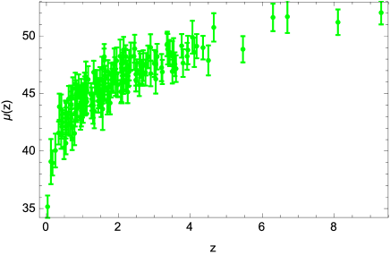
Figure 1: Distance modulus $\mu(z)$ for the calibrated GRB Hubble diagram obtained by fitting the $E_{\rm p,i}$ – $E_{\rm iso}$ relation.

Table 1: Some data used in our analysis.

Some GRBs observable quantities
redshift	$E_{\rm p,i}(keV)$	$\sigma_{E_{\rm p,i}}$	$S_{bolo}(10^{-6}\,erg\,cm^{-2})$	$\sigma_{S_{bolo}}$	$E_{\rm iso}(10^{52}\,erg)$	$\sigma_{E_{\rm iso}}$
0.03351	4.9	0.49	20.6219	2.06219	0.00535399	0.000535399
0.125	55.	45.	52.6588	21.0635	0.216774	0.0867097
0.1685	82.	8.2	204.139	20.4139	1.61591	0.161591
0.25	3.37	1.79	0.127068	0.0317671	0.00244119	0.000610299
0.31	203.	53.	207.837	41.5672	6.55552	1.3111
0.3399	1250.	150.	2349.65	335.665	91.8909	13.1273
0.36	1060.	275.	178.062	48.9183	7.97042	2.18968
0.41	70.	21.	11.3826	2.88168	0.693324	0.175525
0.414	440.	180.	43.6518	8.44872	2.72107	0.526658
0.434	93.	15.	9.82091	1.88864	0.685192	0.131768
0.45	129.	26.	12.7073	1.27073	0.966894	0.0966894
0.4791	81.3505	8.13505	13.1412	1.31412	1.16253	0.116253
0.49	51.	5.1	17.6258	1.8851	1.64622	0.176066
0.5295	61.	15.	1.56474	0.156474	0.176323	0.0176323

4.2 H(z) measurements

The measurement of the Hubble parameter is a complementary probe to constrain the cosmological parameters and investigate the dark energy. The Hubble parameter can be measured using the so-called cosmic chronometers. The most reliable cosmic chronometers at present are old early-type galaxies that evolve passively on a timescale much longer than their age difference, which formed the vast majority of their stars rapidly and early and have not experienced subsequent major episodes of star formation or merging. We used a list of $28$ $H(z)$ measurements obtained in this way that were compiled in farooqb .

4.3 Constraints from the growth rate data

It is known Percival05 that the growth factor of density perturbations satisfies the following differential equation on subhorizon scales ($k^{2}\gg a^{2}H^{2}$), where primes denote differentiation with respect to the scale factor $a$

$$\delta^{\prime\prime}(a)+\left(\frac{3}{a}+\frac{H^{\prime}(a)}{H(a)}\right)\delta^{\prime}(a)-\frac{3}{2}\frac{\Omega_{m}}{a^{5}H(a)^{2}/H_{0}^{2}}\,\delta(a)=0\,,$$ (37)

where $\delta(a)=\frac{\delta\rho_{m}}{\rho_{m}}$ denotes the cosmological matter overdensity . This differential equation has in general two solutions that correspond to two modes, a growing and a decaying one, that in a matter dominated universe scale as $\delta=a$ and as $\delta=a^{-3/2}$ respectively. In order to numerically integrate the Eq. (37), we set the usual initial conditions: $\delta(a_{in})\simeq a_{in}$ and $\delta^{\prime}(a_{in})\simeq 1$. The growth rate is defined as $f(a)=\displaystyle{\frac{d\delta(a)}{d\log a}}$. Most of the growth rate data are provided by peculiar velocity measurements in galaxy surveys and are obtained in terms of galaxy density, which is related to the matter perturbation by the relation $\delta_{g}=b\delta_{m}$, where $b$ is the so called (unknown) bias parameter. Therefore measurements of $f$ depend on the value of the bias parameter. A more reliable function is the product $f(z)\sigma_{8}(z)=f\sigma_{8}(z)$ where $\sigma_{8}(z)$ is the amplitude of the power spectrum of density perturbations on the scale $8h^{-1}$Mpc, as it is independent on the bias and can be measured also from weak lensing surveys. Here we use the Gold-2017 compilation of 18 $f\sigma_{8}(z)$ measurements, presented in Nesseris2017 . It is worth noting that to use the Gold-2017 growth data we follow the same procedure as explained in Nesseris2017 to correct the data for the Alcock-Paczynski effect mentioned in that paper. Actually the growth rate data depend on the fiducial model used to convert redshifts to distances. Following Nesseris2017 we rescaled the measurements by the ratios of $H(z)d_{A}(z)$ of our model to that of the fiducial one.

5 Statistical analysis

To constrain the parameters of the GPS dark energy model we performed a preliminary and standard fitting procedure to maximize the likelihood function ${\cal{L}}({\bf p})$. This requires the knowledge of the precision matrix, that is, the inverse of the covariance matrix of the measurements,

$$\footnotesize{\cal{L}}({\bf p}) \propto \frac{\exp{(-\chi^{2}_{SNIa/GRB}/2)}}{(2\pi)^{\frac{{\cal{N}}_{SNIa/GRB}}{2}}|{\bf C}_{SNIa/GRB}|^{1/2}}\frac{\exp{(-\chi^{2}_{H}/2})}{(2\pi)^{{\cal{N}}_{H}/2}|{\bf C}_{H}|^{1/2}}$$

$$\frac{\exp{(-\chi^{2}_{f\sigma_{8}}/2)}}{(2\pi)^{\frac{{\cal{N}}_{f\sigma_{8}}}{2}}|{\bf C}_{f\sigma_{8}}|^{1/2}}\,,$$

where

$$\chi^{2}(\bf p)=\sum_{i,j=1}^{N}\left(x^{\rm d}_{i}-x^{th}_{i}(p)\right)C^{-1}_{ij}\left(x^{\rm d}_{j}-x^{th}_{j}(p)\right)\,.$$ (38)

Here $\bf p$ is the set of parameters, $N$ is the number of data points, $\bf x^{\rm d}_{i}$ is the $i-th$ measurement; $\bf x^{th}_{i}(p)$ indicates the theoretical prediction for this measurement, it depends on the parameters $\bf p$;, $\bf C_{ij}$ is the covariance matrix (specifically,
${\bf C}_{SNIa/GRB/H/f\sigma_{8}}$ indicates the SNIa/GRBs/H/$f\sigma_{8}$ covariance matrix). Moreover we use a gaussian prior term $\frac{1}{\sqrt{2\pi\sigma^{2}}}\exp{\left[-\frac{1}{2}\left(\frac{h-h_{peak}}{\sigma}\right)^{2}\right]}$, where shoes

$$h_{peak}=h_{shoes}\,,$$ (39)

$$\sigma=5\sigma_{h_{shoes}}\,.$$

It is worth to stress that in Tables (3) and (5) the inferred value of $h$ is strongly influenced by this prior, because neither SNIa, nor GRB, nor $f\sigma_{8}(z)$ data sets by itself do not allow us to determine $h$. To sample the ${\cal{N}}$ dimensional space of parameters, we use the MCMC method and ran three parallel chains and use the Gelman - Rubin diagnostic approach to test the convergence. As a test probe, it uses the reduction factor $R$, which is the square root of the ratio of the variance between-chains and the variance within-chains. A large $R$ indicates that the variance between-chains is substantially greater than the variance within-chain, so that a longer simulation is needed. We require that $R$ converges to 1 for each parameter. We set $R-1$ to be of order $0.1$. We discarded the first $30\%$ of the point iterations at the beginning of any MCMC run, and thinned the chains that were run many times. We finally extracted the constrains on the parameters by coadding the thinned chains. The histograms of the parameters from the merged chains were then used to infer median values and confidence ranges: the $15.87$th and $84.13$th quantiles define the $68\%$ confidence interval; the $2.28$th and $97.72$th quantiles define the $95\%$ confidence interval; and the $0.13$th and $99.87$th quantiles define the $99\%$ confidence interval. In Tables (2), (3) we present results of our analysis. In Figs. (3) and (2) we plot respectively the behaviour of the GPS equation of state and the $\Omega$s parameters corresponding to the best fit values of the parameters.

	GPS Dark energy
$Id$	$\langle x\rangle$	$\tilde{x}$	$68\%\ {\rm CL}$	$95\%\ {\rm CL}$	$\langle x\rangle$	$\tilde{x}$	$68\%\ {\rm CL}$	$95\%\ {\rm CL}$
	SNeIa/GRBs/H(z)/ $f\sigma_{8}(z)$				SNeIa/H(z)/$f\sigma_{8}(z)$
$\Omega_{m}$	0.27	0.27	(0.25, 0.31)	(0.22, 0.32)	0. 295	0.3	(0.28, 0.32)	(0.25, 0.34)
$w_{0}$	-1.13	-1.14	(-1.3, -0.96)	(-1.4, -0.78)	-0.99	-0.98	(-1.12, -0.84)	(-1.27, -0..73)
$\alpha$	3.0	2.8	(2.1, 4.2)	(2.05, 4.8)	2.9	2.8	(-2.17, 3.5)	(2.01, 4.4)
$\beta$	0.07	0.08	(0.03, 0.11)	(0.02, 0.16)	0.08	0.08	(0.05,0.11)	(0.02, 0.16)
$h$	0.70	0.7	(0.69, 0.71)	(0.67, 0.72)	0.71	0.71	(0.69, 0.71)	(0.68, 0.73)

Table 2: Constraints on the GPS parameters from different data: combined SNIa and GRBs Hubble diagrams, $f\sigma_{8}(z)$ data sets and $H(z)$ data sets (Left Panel); and SNIa Hubble diagram, $f\sigma_{8}(z)$ data sets and $H(z)$ data sets (Right Panel ). Columns report the mean $\langle x\rangle$ and median $\tilde{x}$ values and the $68\%$ and $95\%$ confidence limits.

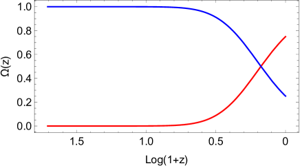
Figure 2: Redshift evolution of the $\Omega$s parameters for the GPS model, corresponding to the best fit values of model parameters. The blue line represents $\Omega_{m}(z)$, and the red line $\Omega_{GPS}(z)$

6 Confrontation of the GPS model with the cosmological constant model of dark energy

	GPS Dark energy
$Id$	$\langle x\rangle$	$\tilde{x}$	$68\%\ {\rm CL}$	$95\%\ {\rm CL}$
	SNeIa/GRBs/ $f\sigma_{8}(z)$
$\Omega_{m}$	0.20	0.21	(0.17, 0.23)	(0.15, 0.31)
$w_{0}$	-1.1	-1.14	(-1.2, -0.97)	(-1.4, -0.88)
$\alpha$	2.8	2.7	(2.1, 3.6)	(2.02, 4.2)
$\beta$	0.04	0.03	(0.02, 0.06)	(0.02, 0.1)
$h$	0.69	0.69	(0.69, 0.7)	(0.68, 0.72)

Table 3: Constraints on the GPS parameters from SNIa and GRBs Hubble diagrams, and $f\sigma_{8}(z)$ data sets. Columns report the mean $\langle x\rangle$ and median $\tilde{x}$ values and the $68\%$ and $95\%$ confidence limits.

It is interesting to compare predictions of the GPS model of dark energy with predictions of the Standard $\Lambda$CDM model that relates the observed accelerated expansion of the Universe to the non-zero value of the cosmological constant.

When the accelerated expansion of the Universe is due to the cosmological constant the dark energy equation of state is $p_{DE}=-\varrho_{DE}$, so $w=-1$. From the continuity equation (4) it follows that $\varrho_{DE}={\rm const}$. In this case at the post-recombination epoch assuming spatially flat $\Lambda$CDM model we have

$$H^{2}(z)=H^{2}_{0}\big{(}\Omega_{m}(1+z)^{3}+1-\Omega_{m}\big{)}\,.$$ (40)

Using this Hubble expansion rate the luminosity distance $d_{L}$ and the angular diameter distance $d_{A}(z)$ are defined as

$$d_{L}(z) = \frac{c}{H_{0}}(1+z)\int_{0}^{z}\frac{dy}{\sqrt{1-\Omega_{m}+\Omega_{m}(y+1)^{3}}},$$ (41)

$$d_{A}(z) = \frac{c}{H_{0}}\frac{1}{1+z}\int_{0}^{z}\frac{dy}{\sqrt{1-\Omega_{m}+\Omega_{m}(y+1)^{3}}},$$ (42)

Using this luminosity distance, we can evaluate the distance modulus from its standard definition

$$\mu(z)=25+5\log{d_{L}(z)}\,.$$ (43)

In Table (4) and (5) we present results of the same statistical analysis as performed for the GPS model for the $\Lambda$CDM model, using the same data sets. It turns out that $\mu^{GPS}_{0}\simeq 0.68$, and $\mu^{\Lambda CDM}_{0}\simeq 0.7$.

	$\Lambda$CDM
$Id$	$\langle x\rangle$	$\tilde{x}$	$68\%\ {\rm CL}$	$95\%\ {\rm CL}$	$\langle x\rangle$	$\tilde{x}$	$68\%\ {\rm CL}$	$95\%\ {\rm CL}$
	SNeIa/GRBs/H(z)/$f\sigma_{8}(z)$				SNeIa/H(z)/$f\sigma_{8}(z)$
$\Omega_{m}$	0.26	0.26	(0.24, 0.28)	(0.22, 0.3)	0. 25	0.25	(0.25, 0.27)	(0.23, 0.32)
$h$	0.70	0.70	(0.69, 0.71)	(0.68, 0.72)	0.72	0.72	(0.69, 0.73)	(0.68, 0.74)

Table 4: Constraints on the $\Lambda$CDM parameters from different data: combined SNIa and GRBs Hubble diagrams, $f\sigma_{8}(z)$ data sets and $H(z)$ data sets (Left Panel); and SNIa Hubble diagram, $f\sigma_{8}(z)$ data sets and $H(z)$ data sets (Right Panel). Columns report the mean $\langle x\rangle$ and median $\tilde{x}$ values and the $68\%$ and $95\%$ confidence limits.

	$\Lambda$CDM
$Id$	$\langle x\rangle$	$\tilde{x}$	$68\%\ {\rm CL}$	$95\%\ {\rm CL}$
	SNeIa/GRBs/ $f\sigma_{8}(z)$
$\Omega_{m}$	0.23	0.23	(0.19, 0.26)	(0.17, 0.29)
$h$	0.69	0.7	(0.69, 0.7)	(0.67, 0.73)

Table 5: Constraints on the $\Lambda$CDM parameters from SNIa and GRBs Hubble diagrams, and $f\sigma_{8}(z)$ data sets. Columns report the mean $\langle x\rangle$ and median $\tilde{x}$ values and the $68\%$ and $95\%$ confidence limits.

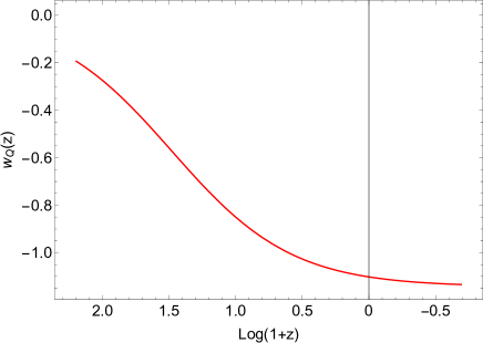
Figure 3: Redshift evolution of the equation of state for the $GPS$ model, corresponding to the best fit values of model parameters, when the full dataset is used.

7 Discussion of our calibration procedure of the $E_{\rm p,i}$ – $E_{\rm iso}$ relation

In this section we discuss the reliability, for cosmological applications, of our calibration technique of the $E_{\rm p,i}$ – $E_{\rm iso}$ relation, based on Type Ia supernovae Hubble diagram. We are specially interested in understanding how much this calibration procedure affects the independence of the (SNIa and GRBs) datasets. We already discussed this topic in some previous papers (see MGRB1 and references therein). However, in order to further investigate this question we performed an independent calibration, based on an approximate formula for the luminosity distance which holds in any cosmological model, and not on a power series expansion in the redshift parameter z, as in the cosmographic approach. Our starting point is the well known relation between the angular diameter distance $d_{A}$ and the luminosity distance $d_{L}$

$$d_{L}=\left(1+z\right)^{2}d_{A},$$ (44)

where the angular diameter distance $d_{A}$ is a solution of the equation

$$\left(\frac{dz}{dv}\right)^{2}\frac{d^{2}d_{A}}{dz^{2}}+\left(\frac{d^{2}z}{dv^{2}}\right)\frac{dd_{A}}{dz}+\frac{4\pi G}{c^{4}}T_{\alpha\beta}k^{\alpha}k^{\beta}d_{A}=0.$$ (45)

with the following initial conditions:

$$d_{A}(z)\arrowvert_{z=0}=0,$$

(46)

$$\frac{dd_{A}(z)}{dz}\arrowvert_{z=0}=\frac{c}{H_{0}}.$$

In Eq. (45) $\it{v}$ is the affine parameter, $T_{\alpha\beta}$ is the matter density tensor, $k^{\alpha}=\displaystyle{{dx^{\alpha}\over dv}}=-g^{\alpha\beta}\Sigma,_{\beta}$ is the vector field tangent to the congruence of light rays, and $\Sigma$ is the null surface along which the light rays propagate from the source. In the general form this equation is very complicated (Kant98 ; Kant20 ; Kant01 ; approx ), and in most cases it does not admit analytical solution. From the mathematical point of view it turns out that it is of Fuchsian type with several regular singular points and a regular singular point at infinity. When we introduced the dimensionless angular diameter distance $r=d_{A}H_{0}/c$ we discovered approx that there is a simple function, which quite accurately reproduces the exact numerical solutions of the equation (45) for $z$ up to high values. Here we generalize this function, to extend the accuracy of this approximation up to $z\simeq 10$. This function $r(z)$ has the form

$$r(z)=\frac{z(z+1)^{2}}{\sqrt{d_{3}z^{3}+\left(d_{2}z^{2}+d_{1}z+1\right){}^{2}}}\,.,$$ (47)

where $d_{1}$, $d_{2}$ and $d_{3}$ are constants that depend on parameters of the considered cosmological model. Moreover the function (47) automatically satisfies the imposed initial conditions, so $r(0)=0$ and $\displaystyle{dr\over dz}(0)=1$.

This approximate expression immediately provides an empirical formula for the approximate luminosity distance. The GRBs and the SNIa samples have been fitted simultaneously with this approximated luminosity function. For what it concerns the GRBs sample, our task is to determine the parameters $\{a,b,d_{1},d_{2},d_{3}\}$. Actually the $E_{\rm p,i}$ – $E_{\rm iso}$ relation can be written in the form

$$\log_{10}S_{\rm bol}=a+b\log_{10}E_{\rm p,i}-\log_{10}[4\pi{d^{2}_{L\,approxi}}(z,d_{1},d_{2},d_{3})].$$ (48)

To efficiently sample the $5$-dimensional parameter space, we used the MCMC method and ran three parallel chains and used the Gelman-Rubin convergence test, as described in the previous section. It turns out that the calibration parameters $a$, $b$, and $\sigma$ are fully consistent with the results obtained from the SNIa sample based calibration (see MGRB1 ) , confirming the reliability of our calibration technique : we actually find that$a=1.87\pm 0.09$  $\sigma_{\rm int}=0.36_{-0.02}^{+0.03}$  $b=52.5_{-0.1}^{+0.13}$, $d_{1}=1.17^{+0.11}_{0.1}$, $d_{2}=0.33^{+0.04}_{-0.05}$ and $d_{3}=0.2^{+0.2}_{-0.1}$. It is worth noticing that the Eq. (48) can be used also in a full Bayesian procedure to estimate the cosmological parameters and the additional parameters of the $E_{\rm p,i}$ – $E_{\rm iso}$ correlation MGRB1 ; MEC11 . However it is clear that in this case the values of the correlation parameters, which are important for cosmological applications, unfortunately depend on the assumed background cosmological model, so they do not provide an independent calibration.

8 Comparison of the GPS model with the $\Lambda$CDM model

To compare the different models presented in the previous sections with the data and to check if we can discriminate them, we use the Akaike Information Criterion (AIC) aic aic2 , and its indicator

$$AIC=-2\ln{\cal{L}_{\bf max}}+2k_{p}+\frac{2k_{p}(k_{p}+1)}{N_{tot}-k_{p}-1}\,,$$ (49)

where $N_{tot}$ is the total number of data and $k_{p}$ the number of free parameters (of the cosmological model). In our case we have $N_{tot}=815$, and $k_{p}=6$. It turns out that the smaller is the value of AIC the better is the fit to the data. To compare different cosmological models we introduce the model difference $\Delta_{AIC}=AIC_{model}-AIC_{min}$. The relative difference corresponds to different cases: $4<\Delta_{AIC}<7$ indicate a positive evidence against the model with higher value of $AIC_{model}$, while $\Delta_{AIC}\geq 10$ indicate a strong evidence. If, $\Delta_{AIC}\leq 2$ is an indication that the two models are consistent. In our case we have found that the model with the lower AIC is the GPS model and $\Delta_{AIC}=0.7$ if we consider GRBs, and $\Delta_{AIC}=5.7$ without GRBS. This result indicates that the two models are statistically consistent, if we consider GRBs data, and that the $\Lambda$CDM model would be slightly favoured without GRBs.

9 Conclusions

We have compared two different models of dark energy with presently available observational data. We show that with appropriate choice of the parameters of these models they are compatible with observations. Our statistical analysis indicates that the GPS model seems to be slightly more favoured than the $\Lambda$CDM model, if we consider the GRBs Hubble diagram. It means that to further restrict different models of dark energy it will be necessary to increase the precision of the Hubble diagram at high redshifts, and to perform more detailed analysis of the influence of dark energy on the process of formation of large scale structure and in particular on its late evolution at $z<2$. Of course, more and more precise observational data will reduce statistical errors and could lead to further restrictions on parameters describing properties of dark energy and better differentiate different models.

10 Acknowledgments

MD is grateful to the INFN for financial support through the Fondi FAI GrIV. EP acknowledges the support of INFN Sez. di Napoli (Iniziativa Specifica QGSKY).

References

- (1) Y.B. Zeldovich, Sov. Phys. Usp. 11, 381, (1968)
- (2) M. Demianski, E. Piedipalumbo, D. Sawant, L. Amati, Astronomy & Astrophysics, 598, A113 (2017)
- (3) O. Farroq, B. Ratra, ApJ, 766, L7 (2013)
- (4) A.G. Riess, A.V. Filippenko, P. Challis, A. Locchiatti, A. Diercks, et al., 1998, Astron. J., 116, 1009 (1998)
- (5) S. Perlmutter, G. Aldering , G. Goldhaber, R. A. Knop, P. Nugent, et al., Astrophys. J. 517, 565 (1999)
- (6) Suzuki et al. (The Supernova Cosmology Project), ApJ, 746, 85 (2012)
- (7) L. Amati, C. Guidorzi, F. Frontera, M. Della Valle, F. Finelli, R. Landi, R. E. Montanari, MNRAS, 391, 577 (2008)
- (8) M. Demianski, E. Piedipalumbo, D. Sawant, L. Amati, Astronomy & Astrophysics, 598, A112 (2017)
- (9) E. Aubourg., et al. (BOSS Collaboration), Phys. Rev. D 92, 123516 (2015)
- (10) Planck Collaboration, Planck 2015 results. XIII. Cosmological parameters, Astronomy & Astrophysics, 594, A13 (2015)
- (11) W.J. Percival, Astronomy & Astrophysics 443, 819 (2005)
- (12) A.G. Riess, L. Macri, Li W. Lampeitl, H. Casertano, et al. ApJ, 699, 539 (2009)
- (13) A. G Riess, L.M. Macri, S.L Hoffmann, D., Scolnic, S. Casertano, et al., ApJ, 826, 56R (2016)
- (14) A. Joyce, L. Lombriser and F. Schmidt, Annu. Rev. Nucl. Part. Sci., 66, 95 (2016)
- (15) M. Demianski, E. Piedipalumbo, C. Rubano, MNRAS, 411, 1213 (2011)
- (16) E. Piedipalumbo, P. Scudellaro, G. Esposito, C. Rubano, General Relativity and Gravitation, 44, 2611 (2012)
- (17) D. Glavan, T. Prokopec and A.A. Starobinsky, Eur. Phys, J. C78, 371 (2018)
- (18) B. Boisseau, G. Esposito-Farese, D. Polarski, A. A. Starobinsky, Phys. Rev. Lett. 85, 2236 (2000)
- (19) S. Nesseris, G. Pantazis, L. Perivolaropoulos, Phys. Rev. D 96, 023542 (2017)
- (20) R. Kantowski, ApJ, 507, 483 (1998)
- (21) R. Kantowski, J. K. Kao, R. C. Thomas, ApJ, 545, 549 (2000)
- (22) R. Kantowski, and R. C. Thomas, ApJ, 561, 491 (2001)
- (23) M. Demianski, R. de Ritis, A. A. Marino, E. Piedipalumbo, A&A, 411, 33 (2003)
- (24) H. Akaike, 1974, IEEE Transactions on Automatic Control 19, 716 (1974)
- (25) A.R. Liddle, MNRAS, 377, L74 (2007)