Manifestation of classical nonlinear dynamics in optomechanical entanglement with a parametric amplifier

Abstract

Cavity optomechanical system involving an optical parametric amplifier (OPA) can exhibit rich classical and quantum dynamical behaviors. By simply modulating the frequency of the laser pumping the OPA, we find two interesting parameter regimes, with one of them enabling to study quantum-classical correspondence in system dynamics, while there exist no classical counterparts of the quantum features for the other. For the detuning of the laser pumping around the mechanical frequency, as the parametric gain of OPA increases to a critical value, the classical dynamics of the optical or mechanical modes can experience a transition from the regular periodic oscillation to period-doubling motion, in which cases the light-mechanical entanglement can be well studied by the logarithmic negativity and can manifest the dynamical transition in the classical nonlinear dynamics. In addition, the optomechanical entanglement shows a second-order transition characteristic at the critical parametric gain. For the laser detuning being about twice the mechanical frequency, the kind of normal mode splitting comes up in the laser detuning dependence of optomechanical entanglement, which is induced by the squeezing of the optical and mechanical hybrid modes and finds no classical correspondence. The OPA assisted optomechanical systems therefore offer a simple way to study and exploit quantum manifestations of classical nonlinear dynamics.

I INTRODUCTION

To seek for and explore quantum manifestations of classical nonlinear dynamics is one of the most fundamental problems in physics. The familiar dynamical behaviors, such as period-doubling, quasi-periodicity motions and chaos Bak_prl2015 ; Ott_PT1994 ; Wang_prl2014 , which are very common in classical nonlinear systems, can usually find their counterparts in quantum systems. However, the quantum signature of classical nonlinear dynamics may be found in different parameter regimes, leading to inconsistent experimental requirements in studying classical and quantum dynamics. For instance, some of the quantum chaotic problems, such as energy level-spacing statistics Berr_Math1986 and quantum chaotic scattering Lai_ibid1992 , can only be addressed in the limit of low dimensional Hamiltonian Haa_b2010 . On the other hand, quantum entanglement EPR_1935 , which is a fundamental phenomenon in quantum mechanics, describes nonlocal two-body or many-body correlations in a form of quantum superposition. However, the non-locality of quantum entanglement has no classical correspondence. Much attention then has been paid to the interplay between classical nonlinear dynamics and quantum dynamical behaviors. Previous works have found that the quantum-classical correspondence in the entanglement dynamics can be analyzed from the perspective of classical trajectories and be calculated by the reduced density linear entropy Zhang_pra2008 , and the quantum-phase transition in the Dicke model is accompanied by the emergence of an entanglement singularity Lambert_PRL2004 . In addition, the connections between classical collective dynamics and quantum entanglement are widely studied in coupled qubit-resonator systems Zhirov_prb2009 , trapped ions Lee_PRL2013 , and optomechanical systems Wang_prl2014 .

Cavity optomechanics is associated with light-oscillator interacting systems consisting of an optical cavity and a mechanical mirror As_Aspel_RMP2014 ; as_Mar_prl2007 ; as_Rae_prl2007 ; as_Teufel_Nature2011 ; as_Rabl_prl2011 ; as_Xu_pra2013 ; as_Li_oe2017 . When the cavity is driven by an introduced input laser, the awakened cavity will exert a radiation pressure on the movable mirror and make it oscillate. Conversely, the oscillating mirror changes the length of the cavity and thus the cavity intensity dependent radiation pressure force, giving rise to the optomechanical coupling. Various interesting quantum phenomena have been observed in optomechanical systems Blen_Phys2000 ; non_tan_pra2014 ; non_Liao_prl2016 ; non_Li_pra2018 , such as light-mechanical entanglement Vitali_prl2007 ; EN_Wnag_prl2018 ; EN_Chen_pra2014 ; EN_Liao_pra2015 ; EN_Li_prl2018 ; Macini_pra1997 ; Bose_pra1999 ; Zhang_pra2003 ; Pinard_EL2005 and squeezed states La_Sci2004 ; sq_Kronwald_pra2013 ; sq_EE_Sci2015 ; sq_Lei_prl2016 ; Aga_pra2016 ; sq_Hu_pra2018 . On the other hand, since the optomechanical coupling is intrinsically nonlinear, the systems are good candidates for studying nonlinear dynamical behaviors. Early experimental demonstration of chaotic dynamics has been done by Carmon et al. Car_prl2007 . Before the dynamics becomes chaotic, these optomechanical system may also experience some times of period-doubling, going through the regular route from periodic oscillations to quasi-periodicity, as discussed in some recent works Larson_pra2011 ; Ma_pra2014 ; Lv_prl2015 . Moreover, a multi-mode optomechanical system may exhibit collective dynamics, such as synchronization and anti-phase synchronization Bem_pra2017 ; Mari_prl2013 ; Lud_prl2013 ; Liao_pra2019 , and as mentioned before, studies by using optomechanical systems as a paradigm to address the correspondence between optomechanical entanglement and synchronization have also been examined Ying_pra2014 . In particular, strong fingerprints of periodic oscillations and quasi-periodic motion in the quantum entanglement can be found Wang_prl2014 .

To search for the correspondence between entanglement dynamics and classical nonlinear motion, we consider a composite cavity optomechanical setting, in which an optical parametric amplifier (OPA) is involved. The OPA, a second-order optical crystal in nature, has many applications in both classical and quantum optics. In the classical case, it is used to transform laser light into almost any (optical) frequency. From a quantum point of view, the pairs of down-converted photons generated by OPA can show nearly perfect single- or dual-squeezing Gerry_book2005 . Therefore, the interplay between optomechanics and OPA is naturally a significant topic to study the nonlinear quantum dynamics. The OPA can modify the dynamical instabilities and nonlinear dynamics of the system Pina_pra2016 ; Huang_pra2009_spll . Moreover, it has also found applications in generating strong mechanical squeezing Aga_pra2016 ; sq_Hu_pra2018 , enhancing optomechanical cooling Huang_pra2009 , and increasing single-photon optomechanical coupling LV_prl2015_114 .

We envision a two-field driving scenario, with one of them driving the cavity and the other pumping the OPA. By scanning the laser frequency of the OPA pumping, we find two interesting regimes. First, we find good quantum-classical correspondence between the light-mechanical entanglement and the classical nonlinear dynamics for the laser detuning of OPA around the mechanical frequency. In this regime, when the classical behavior transits from the regular periodic oscillation to period-doubling motion as the parametric gain of OPA increases, the light-mechanical entanglement dynamics also exhibits regular periodic oscillation and period-doubling motion, in correspondence to the respective classical behavior. In particular, we find a critical point $\Lambda_{c}$ for the transition from periodic motion to period-doubling motion, which is related to an entanglement singularity, namely, the light-mechanical entanglement continuously enhances with the increase of the OPA gain, but its derivative with respect to the parametric gain is discontinuous. This characteristic is in resemblance to a second-order quantum phase transition. Second, while the laser pumping of OPA is detuned from cavity resonance by twice the mechanical frequency, the light-mechanical entanglement exhibits normal mode splitting kind of feature, which can be explained via the hybrid mode squeezing principle. Our result gives a nice example of the manifestation of classical nonlinear dynamics in optomechanical entanglement by simply modulating the OPA pumping, and can be easily tested by the state-of-the-art cavity optomechanical systems.

The rest of this paper is organized as follows. We first introduce the optomechanical setup in Sec. II and then discuss the classical dynamics in Sec. III. In Sec. IV, we introduce the measure of the optomechanical entanglement and discuss the interesting physics with the laser pumping of OPA around twice the mechanical frequency. In Sec. V, we discuss both the quantum and classical dynamical behavior for the laser pumping of OPA around the mechanical frequency, and show the evidence for quantum-classical correspondence. We finally summarize our result in Sec. VI.

II MODEL

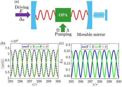
Figure 1: (Color online) (a) Sketch of the optomechanical system under two-field driving. The cavity is driven by an external driving laser with strength $E$ and detuning $\Delta_{0}$, and the OPA inside the cavity is pumped by another laser field. (b) Long-time behavior of the cavity field strength $|\langle a(t)\rangle|$ and (c) the light-mechanical entanglement $E_{N}$ with $\tau=2\pi/\Omega$ for a typical set of experimental parameters Tho_Nat2008 : $(E,g,\gamma_{m},\kappa,\Delta_{0})/\omega_{m}=(6\times 10^{4},4\times 10^{-6},10^{-6},0.2,1)$. The OPA is pumped with the parametric gain $\Lambda/\omega_{m}=0.02$, the detuning $\Omega/\omega_{m}=1.16$, and the parametric phase $\theta=0,\text{ $\pi$}$. Note that the mechanical thermal noise is not taken into account so far (i.e. $n_{m}=0$), however, it can be detrimental for experimental generation of the optomechanical entanglement, see the Sec. V for further discussions. For current consideration, the analytical approximation of the classical mean values (dash) shows nice agreement with the numerical solution.

We consider an optomechanical system with a degenerate optical parametric amplifier (OPA) inside the Fabry-Perot cavity with one fixed partially transmitting mirror and one movable totally reflecting mirror, as shown in Fig. 1. Supposing that the length of the cavity is $L$ in the rest and the finesse is represented by $F$, which leads to a photon decay rate given by $\kappa=\pi c/(2FL)$. The movable mirror is treated as a quantum-mechanical harmonic oscillator with effective mass $m$, frequency $\omega_{m}$, and energy decay rate $\gamma_{m}$. We assume that the cavity mode with the resonant frequency $\omega_{c}$ is driven by an external laser of the frequency $\omega_{l}$ and the amplitude $E=\sqrt{2\kappa P/\hbar\omega_{l}}$, depending on the laser power $P$. On the other hand, the degenerate OPA is pumped by another laser field at frequency $2\omega_{p}$, giving rise to a parametric gain denoted by $\Lambda e^{i\theta}$, which is determined by the strength and the phase of the pumping laser. The total Hamiltonian of the system in the rotating frame at the laser frequency $\omega_{l}$ is given by

$$H = \hbar\Delta_{0}a^{\dagger}a+\frac{\hbar\omega_{m}}{2}(p^{2}+q^{2})-\hbar ga^{\dagger}aq+i\hbar E(a^{\dagger}-a)$$ (1)

$$+i\hbar\Lambda(e^{i\theta}a^{\dagger 2}e^{-i\Omega t}-e^{-i\theta}a^{2}e^{i\Omega t}).$$

Here, $\Delta_{0}=\omega_{c}-\omega_{l}$ and $\Omega/2=\omega_{p}-\omega_{l}$ are the detunings of the driving laser frequency from the cavity resonance and the down-conversion photon frequency; $a$ and $a^{\dagger}$ are the annihilation and creation operators of the cavity mode, respectively; $q$ and $p$ are the position and momentum operators for the movable mirror, satisfying the standard canonical commutation relation $[q,\>p]=i\hbar$; and $g$=$x_{ZPF}\omega_{c}/L$ is the single-photon optomechanical coupling strength arisen from the radiation pressure force with $x_{ZPF}=\sqrt{\frac{\hbar}{2m\omega_{m}}}$ being the zero point motion of the mechanical mode. In Eq. (1), the first and second terms are the free energies of the cavity mode and the mechanical oscillator, respectively; the third term describes the radiation-pressure induced coupling between the cavity and the mechanical mode; the fourth term describes the longitudinal cavity driving, and the last term represents the OPA pumping, leading to the generation of pairs of cavity photons.

Using the Heisenberg equations of motion for the cavity and mechanical operators and taking the mechanical damping and cavity decay into account, the dynamics of the system can be described by the following set of quantum Langevin equations Bar_book2004

$$\dot{q} = \omega_{m}p,$$

$$\dot{p} = -\omega_{m}q-\gamma_{m}p+ga^{\dagger}a+\xi(t),$$

$$\dot{a} = -(\kappa+i\Delta_{0})a+igaq+E+2\Lambda e^{i\theta}a^{\dagger}e^{-i\Omega t}$$ (2)

$$+\sqrt{2\kappa}a_{in}(t),$$

where $a_{in}$ is the zero-mean vacuum-input noise operator satisfying the auto-correlation function Bar_book2004 $\langle a_{in}^{\dagger}(t)a_{in}(t^{\prime})\rangle=\delta(t-t^{\prime})$, and ${\textstyle\xi}(t)$ is the thermal noise operator acting on the mechanical oscillator. In the regime of high mechanical quality factor $Q\equiv\omega_{m}/\gamma_{m}\gg 1$, the Markovian approximation can be applied to the thermal noise, leading to Giovan_pra2001 $\left\langle\xi(t)\xi(t^{\prime})+\xi(t^{\prime})\xi(t)\right\rangle/2=\gamma_{m}(2n_{m}+1)\delta(t-t^{\prime})$ with $n_{m}=[\exp(\hbar\omega_{m}/k_{B}T)-1]^{-1}$ being the mean thermal excitation number in the mechanical mode and $T$ the thermal bath temperature. Note that, for $\Omega\neq 0$, the parametric interaction here plays a role in resemblance to a periodically amplitude-modulated cavity driving Mari_prl2009 , but the OPA-modulated amplitude depends on the time-varying cavity field itself via the term $\sim 2\Lambda a^{\dagger}$. In the following sections, we focus on the connections between typical dynamical behavior of the classical mean values and the light-mechanical entanglement when the parametric gain and the driving frequency of OPA are especially tuned.

III Classical steady-state behavior

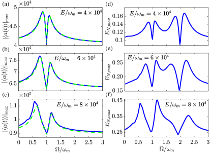
Figure 2: (Color online) $|\langle a(t)\rangle|_{max}$ [(a)-(c)] and $E_{N,max}$ [(d)-(f)] in the long time limit as a function of $\Omega/\omega_{m}$ for driving strengths $E/\omega_{m}=4\times 10^{4}$ [(a),(d)], $E/\omega_{m}=6\times 10^{4}$ [(b),(e)], and $E/\omega_{m}=8\times 10^{4}$ [(c),(f)]. The numerical (analytical) results are presented by the blue solid (green dashed) lines. Other parameters are the same as in Figs. 1(b), 1(c).

We next derive the steady-state solution $\left\langle O(t)\right\rangle$ $(O=q,\,p,\,a)$ for the Eq. (2) via the mean-field theory, where $\left\langle a(t)q(t)\right\rangle=\left\langle a(t)\right\rangle\left\langle q(t)\right\rangle$ and $\left\langle a^{\dagger}(t)a(t)\right\rangle=\left\langle a^{\dagger}(t)\right\rangle\left\langle a(t)\right\rangle$. The equations of motion Eq. (2), which are in analogy to the amplitude-modulated driving schemes sq_Hu_pra2018 ; Fara_pra2012 ; Mari_prl2009 ; Mari_njp2012 , may allow the classical mean values $\left\langle O(t)\right\rangle$ to evolve toward an asymptotic periodic orbit with the periodicity $\tau=2\pi/\Omega$, which can then be analyzed via the Fourier series expansion if the parameters keep the system far from optomechanical instabilities and multistabilities. Since the effectively modulated amplitude $2\Lambda|\langle a^{\dagger}(t)\rangle|\propto 2\Lambda E$ corresponding to OPA pumping ($\sim e^{-i\Omega t}$) in Eq. (2) is much weaker than the driving field $E$, we then derive the steady-state solutions of Eq. (2) in terms of the power series ansatz in $\varepsilon_{s}=2\Lambda E$ as $\left\langle O(t)\right\rangle=\sum_{j=0}^{\infty}\sum_{n=-\infty}^{\infty}O_{n,j}\varepsilon_{s}^{j}e^{in\Omega t}$, with $O_{n,j}$ being time independent coefficients sq_Hu_pra2018 ; Fara_pra2012 ; Mari_prl2009 ; Mari_njp2012 . For weak cavity drivings, we can further rewrite $\left\langle O(t)\right\rangle$ to the first order in $\varepsilon_{s}$ and set $n=0,\pm 1$, leading to Huang_pra2010

$$\left\langle O(t)\right\rangle = O_{0}+\varepsilon_{s}e^{-i\Omega t}O_{+}+\varepsilon_{s}^{*}e^{i\Omega t}O_{-}.$$ (3)

Substituting Eq. (3) into the mean-field version of Eq. (2), it is readily to get the time-independent coefficients $O_{0}$, $O_{+}$, and $O_{-}$

$$p_{0}=0,\quad q_{0}=\frac{g|a_{0}|^{2}}{\omega_{m}},\quad a_{0}=\frac{E}{\kappa+i\Delta},$$ (4)

$$a_{+} = \frac{1}{d(\Omega)\left(\kappa-i\Delta\right)}\{[\kappa-i(\Delta+\Omega)](\omega_{m}^{2}-\Omega^{2}-i\gamma_{m}\Omega)$$ (5)

$$+ig^{2}\omega_{m}|a_{0}|^{2}\}e^{i\theta},$$

$$a_{-}=\frac{ig^{2}\omega_{m}a_{0}^{2}e^{-i\theta}}{d^{*}(\Omega)\left(\kappa+i\Delta\right)},$$ (6)

where $\Delta=\Delta_{0}-gq_{0}$ is the effective detuning and

$$d(\Omega) = -2\Delta g^{2}\omega_{m}|a_{0}|^{2}+[\kappa-i(\Delta+\Omega)][\kappa+i(\Delta-\Omega)]$$ (7)

$$\times(\omega_{m}^{2}-\Omega^{2}-i\gamma_{m}\Omega).$$

Note that the expressions for $q_{\pm}$ and $p_{\pm}$ are not explicitly given since they are unrelated to our discussion in the following. Using the analytical approximations for the steady-state mean values, we show in Fig. 1(b) the comparison of the time-evolutional dynamics with the asymptotic solutions and the full numerical results, which agree well with each other in the weak nonlinear regime. Without loss of generality, the phase of the pumping laser is set to zero in other parts of the paper.

To examine the effect of strong nonlinear dynamics, we plot $|\langle a(t)\rangle|_{max}=\underset{\tau}{max}\{|\langle a(t)\rangle|\}$, which is the maximum of $|\langle a(t)\rangle|$ in one period $\tau$ in the long time limit, as a function of the pumping detuning $\Omega$ in Figs. 2(a)-(c) for gradually increased driving strengths $E$. We find a normal-mode-splitting-like feature, where the separation of the two peaks increases as the driving power enhances. The splitting of $|\langle a(t)\rangle|_{max}$ that arises as a result of the optomechanical coupling $g$ is determined by the structure of the denominator in Eq. (7). Thus, the peaks’ position can be evidenced by the real parts of the roots of $d(\Omega)=0$ in the domain $\text{Re}(\Omega)>0$, as shown in Fig. 3(a). When the driving strength $E$ is small, the real parts of the roots of $d(\Omega)=0$ have two equal values, so no splitting appears. However, there is a splitting in the imaginary part of the roots, i.e. the lifetime splitting Gup_OC1995 , see Fig. 3(b). Increasing the driving strength $E$ to a certain value, the real parts of the roots in the domain $\text{Re}(\Omega)>0$ begin to split. The difference of the two values monotonically increases with the driving strength $E$ being enhanced.

Figure 3: (Color online) (a) The real parts of roots of $d(\Omega)=0$ in the domain $\text{Re}(\Omega)>0$, and (b) the imaginary parts of the roots of $d(\Omega)=0$ as a function of driving $E/\omega_{m}$. Other parameters are the same as in Fig. 2.

In general, the asymptotic solutions Eqs. (4)-(6) can be good approximations of the system steady-state behavior for a wide range of laser detuning $\Omega$ for OPA pumping with $E/\omega_{m}=4\times 10^{4},\text{ }6\times 10^{4}$. While for $E/\omega_{m}=8\times 10^{4}$, the higher-order terms $\sim\varepsilon_{s}^{j}e^{in\Omega t}$ (with $j>1$ or $n>1$) in the Fourier expansion solution should be included for a better fittig. Thus, the first-order approximation Eq. (3) can only provide the proof-of-principle study of the classical nonlinear dynamics. Furthermore, when the cavity intensity $|\langle a(t)\rangle|^{2}$ exceeds the threshold that leads to the instability of mechanical motion, the nonlinear system dynamics cannot be regarded as the quasi-periodic behavior Mari_prl2009 ; Mari_njp2012 and the Fourier expansion solution of the steady-state values $\left\langle O(t)\right\rangle$ will be invalid. The studies in the following thus focus on the parameter regime, where the long-time dynamics of the system is asymptotically periodic and the optomechanical instability is avoided, which will be numerically studied by checking the Routh-Hurwitz criterion while the system’s temporal evolution approaches the dynamical steady state, see further discussions later.

IV Optomechanical entanglement

By linearizing the dynamics around the classical mean values of the operators, i.e. $O(t)=\langle O(t)\rangle+\delta O(t)$, we can find the equations of motion for the quantum fluctuations, which are given by

$$\delta\dot{q} = \omega_{m}\delta p,$$

$$\delta\dot{p} = -\omega_{m}\delta q-\gamma_{m}\delta p+\frac{1}{\sqrt{2}}[G(t)\delta a^{\dagger}+G(t)^{*}\delta a]+\xi(t),$$

$$\delta\dot{a} = -[\kappa+i\Delta(t)]\delta a+\frac{i}{\sqrt{2}}G(t)\delta q+2\Lambda e^{i\theta}\delta a^{\dagger}e^{-i\Omega t}$$ (8)

$$+\sqrt{2\kappa}a_{in}(t),$$

where $G(t)=\sqrt{2}g\left\langle a(t)\right\rangle$ is the photon-number-dependent optomechanical coupling, and $\Delta(t)=\Delta_{0}-g\left\langle q(t)\right\rangle$ is the effective detuning of the cavity resonance from the driving laser frequency. Owing to all of the quantum information is included in Eq. (8) when the system is in the stability regime, one can quantitatively measure the light-mechanical entanglement by the linearized equations. Distinguished from the standard optomechanical system Wang_prl2014 ; Vitali_prl2007 , the OPA can enrich the dynamics of quantum entanglement and allow us to characterize the quantum manifestation of the classical dynamics.

We measure the degree of light-mechanical entanglement by the logarithmic negativity $E_{N}$. For our purposes, we use a vector $u(t)=[\delta q,\delta p,\delta x,\delta y]^{T}$ including the variables of the quantum fluctuations, in which $\delta x=(\delta a+\delta a^{\dagger})/\sqrt{2}$, $\delta y=(\delta a-\delta a^{\dagger})/i\sqrt{2}$ represent the amplitude and phase quadratures of the cavity mode, respectively, with the corresponding noise quadratures being $\delta x_{in}=(\delta a_{in}+\delta a_{in}^{\dagger})/\sqrt{2}$, $\delta y_{in}=(\delta a_{in}-\delta a_{in}^{\dagger})/i\sqrt{2}$. Then the time-dependent equations of motion for the quantum fluctuations can be expressed as $\dot{u}(t)=M(t)u(t)+n(t),$ with the drift matrix

$$M(t)=\left[\begin{array}[]{cccc}0&\omega_{m}&0&0\\ -\omega_{m}&-\gamma_{m}&\text{Re}G(t)&\text{Im}G(t)\\ -\text{Im}G(t)&0&-\kappa+R_{c}(t)&\Delta(t)-R_{s}(t)\\ \text{Re}G(t)&0&-\Delta(t)-R_{s}(t)&-\kappa-R_{c}(t)\end{array}\right],$$ (9)

where $R_{c}(t)=2\Lambda\cos(\Omega t-\theta)$, $R_{s}(t)=2\Lambda\sin(\Omega t-\theta)$ and the input noise $n(t)=[0,\xi(t),\sqrt{2\kappa}\delta x_{in},\sqrt{2\kappa}\delta y_{in}]^{T}$. Without parametric interaction (i.e. $\Lambda=0$), the drift matrix $M$ is time independent, the formal solution for $u(t)$ is simply given by $u(t)=e^{Mt}u(0)+\int_{0}^{t}dt^{\prime}e^{Mt^{\prime}}n(t-t^{\prime})$, and the system is stable and reaches its stationary steady state for $t\rightarrow\infty$ when all the eigenvalues of $M$ have negative real parts. For the time-dependent drift matrix here (i.e. $\Lambda\neq 0$ and $\Omega\neq 0$), the sufficient condition for stability then corresponds to the fact that all eigenvalues of $M(t)$ have negative real parts for the system approaching the long-time periodic dynamics, which associates with the Routh-Hurwitz criterion. While the system is in stable, the optomechanical interaction strength $G(t)$, the effective couplings $-R_{s}\pm\Delta$ and decays $-\kappa\pm R_{c}$ for the cavity quadratures $\delta x,\text{ $\delta$}y$ are then modulated periodically by the OPA pumping, leading to strong fingerprints in the second moments of the quadratures of the classical nonlinear dynamical behaviors.

Due to the zero-mean Gaussian nature of the quantum noises, the equations of motion for $u(t)$ can further be reformulated in terms of the $4\times 4$ covariance matrix $V(t)$ with $V_{k,l}(t)=\langle u_{k}(t)u_{l}^{\dagger}(t)+u_{l}^{\dagger}(t)u_{k}(t)\rangle/2$ and the diagonal noise correlations matrix $D=\text{diag}[0,\gamma_{m}(2n_{m}+1),\kappa,\kappa]$ Mari_prl2009 , leading to $\dot{V}(t)=M(t)V(t)+V(t)M^{T}(t)+D$. To calculate $E_{N}$, the covariance matrix is expressed as a $2\times 2$ sub-block matrices $V(t)=[V_{1},V_{c};V_{c}^{T},V_{2}]$, where $V_{1}$, $V_{2}$, and $V_{c}$ correspond to the mechanical mode, cavity mode, and the optomechanical correlation, respectively Wang_prl2014 . Finally, the logarithmic negativity $E_{N}$ can be calculated by Ying_pra2014

$$E_{N} \equiv \textrm{max}[0,\,-\text{ln}2\eta],$$ (10)

with $\eta\equiv(1/\sqrt{2})[\Sigma(V)-\sqrt{\Sigma(V)^{2}-4\text{det}V}]^{1/2}$ and $\Sigma(V)=\text{det}(V_{1})+\text{det}(V_{2})-2\text{det}(V_{c})$. Since the drift matrix $M(t)$ strongly depends on the parameters $\Lambda,\text{ }\Omega$ of the OPA pumping, the OPA-modulated driven-dissipative dynamics can therefore strongly modify the nonlinear behavior of the optomechanical entanglement. In what follows, we first assume the thermal phonon number to be zero (i.e. $n_{m}=0$), nevertheless, it should be noted that the thermal noise is one of the main detrimental effects to optomechanical entanglement generation in experiments, which will be studied later by considering a finite thermal temperature (see Sec. V).

The temporal dynamics of the light-mechanical entanglement $E_{N}$ is shown in Fig. 1(c), where the time-periodic $E_{N}$ oscillates with the periodicity $\tau=2\pi/\Omega$ in the stable regime, resembling to the mean-field dynamics of $|\langle a(t)\rangle|$. We then quantify the light-mechanical entanglement $E_{N}$ by the maximum in one period $\tau$ Wang_prl2014 ; Fara_pra2012 ; Mari_prl2009 ; Mari_njp2012 namely

$$E_{N,max} = \underset{\tau}{max}\{E_{N}(t)\}.$$ (11)

Similarly, we plot $E_{N,max}$ as a function of the detuning $\Omega$ in Figs. 2(d)-(f) for different driving strengths $E$. By comparing them with the classical result $|\langle a(t)\rangle|_{max}$, one can observe two peaks around $\Omega/\omega_{m}=2$, which are classically nonexistent. To see the insight, we rewrite the effective optomechanical coupling as $G(t)=g_{0}+g_{+1}e^{-i\Omega t}+g_{-1}e^{i\Omega t}$ by using Eq. (3), and assume $g_{0}\propto a_{0}$, $g_{\pm 1}\propto 2\Lambda Ea_{\pm}$ to be positive reals without loss of generality. In fact, the third term $\sim g_{-1}$ can be further neglected when $g_{-1}\ll g_{0},\text{ }g_{+1},\Omega$. Using Eq. (8), and with $\delta q=(\delta b+\delta b^{\dagger})/\sqrt{2}$ and $\delta p=(\delta b-\delta b^{\dagger})/i\sqrt{2}$, the effective linearized Hamiltonian for $\Delta\approx\omega_{m}$ after neglecting the fast oscillating terms becomes $H_{eff}=(-1/2)[g_{0}\delta a\delta b^{\dagger}+g_{+1}e^{i(\Omega-2\omega_{m})t}\delta a\delta b+i2\Lambda e^{-i\theta}e^{i(\Omega-2\omega_{m})t}\delta a^{2}]+H.c$. We then introduce the normal modes $c_{\pm}=(\delta a\pm\delta b)/\sqrt{2}$ and rewrite the Hamiltonian in the interaction picture by rotating with $\left(-g_{0}/2\right)(c_{+}^{\dagger}c_{+}-c_{-}^{\dagger}c_{-})$. Finally, we arrive at

$$H_{eff} \approx \frac{1}{4}g_{\pm}c_{\pm}^{2}+H.c.,$$ (12)

for $\Omega-2\omega_{m}\pm g_{0}=0$, where $g_{\pm}=-(g_{+1}\pm 2i\Lambda e^{-i\theta}$). Eq. (12) which associates with the $squeezing$ of the two hybrid modes $c_{\pm}$ Mari_njp2012 , gives rise to the two peaks around $\Omega/\omega_{m}=2$ in the $\Omega$-dependent light-mechanical entanglement, as shown in Fig. 2 (d)-(f). Owing to $g_{0}\propto E$, the separation of the two peaks increases with the increasing of the driving strength $E$.

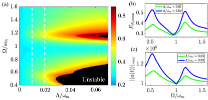
Figure 4: (Color online) (a) $E_{N,max}$ versus the parametric gain $\Lambda/\omega_{m}$ and the detuning $\Omega/\omega_{m}$ for $E/\omega_{m}=8.6\times 10^{4}$. The black area denotes the classically unstable region, confirmed via the Routh-Hurwitz criterion. (b) $E_{N,max}$ and (c) $|\langle a(t)\rangle|_{max}$ versus $\Omega/\omega_{m}$ for parametric gains $\Lambda/\omega_{m}=0.01$ (green) and $\Lambda/\omega_{m}=0.02$ (blue), as indicated by the dashed lines in (a). Other parameters are the same as in Figs. 1(b), 1(c).

On the other hand, it is worthwhile to note that the light-mechanical entanglement $E_{N}$ shows additional ridges near $\Omega/\omega_{m}=1$, which correspond to the positions of the two peaks for the classical mean value of cavity field strength $|\langle a(t)\rangle|_{max}$. Therefore, it allows us to investigate the quantum manifestations of classical nonlinear dynamics by selecting $\Omega$ around $\omega_{m}$. To see stronger nonlinear effects, we will further increase the driving strength $E$, however, the stability of the system will be checked and maintained. In Fig. 4(a), we plot $E_{N,max}$ versus the parametric gain $\Lambda/\omega_{m}$ and the detuning $\Omega/\omega_{m}$ for $E/\omega_{m}=8.6\times 10^{4}$. In the stable regime, the peak values of $E_{N}$ can be found at $\Omega/\omega_{m}\approx 0.55$ and $\Omega/\omega_{m}\approx 1.2$ for different $\Lambda/\omega_{m}$. In addition, $E_{N,max}$ can be improved by increasing $\Lambda$, as shown in Fig. 4(b) and the maximal $E_{N,max}$ is realized in the vicinity of unstable regime with $\Omega/\omega_{m}\approx 1.2$. While for $\Omega/\omega_{m}\approx 0.55$ the system quickly accesses to the unstable regime with the increasing of $\Lambda$ and the entanglement $E_{N,max}$ is much smaller. The classical correspondence is again found in the laser-detuning $\Omega$ dependence of $|\langle a(t)\rangle|_{max}$, see Fig. 4(c).

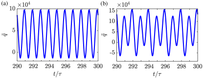
Figure 5: (Color online) Long-time dynamics of the mechanical coordinate $\tilde{q}$, which displays the regular periodic behavior for $\Lambda/\omega_{m}=0.03$, and the period-doubling motion for $\Lambda/\omega_{m}=0.05$ with the two-field detuning being $\Omega/\omega_{m}=1.16$ and the cavity driving strength being $E/\omega_{m}=8.6\times 10^{4}$. Other parameters are the same as in Figs. 1(b), 1(c).

V Quantum manifestations of classical nonlinear dynamics

The classical dynamics discussed in Sec. III is based on the fact that the asymptotic behaviors of the optical mode and mechanical motion are approximately sinusoidal. However, it is known that the system evolution will follow the route, namely, from periodic motion to chaotic behavior when the laser pump of the OPA is gradually increasing. To further study the classical nonlinear behavior, we now use the notations $\tilde{p}$, $\tilde{q}$, and $\alpha=\alpha_{r}+i\alpha_{i}$ for simplicity, which correspond to the mean values $\langle q(t)\rangle$, $\langle p(t)\rangle$ and $\langle a(t)\rangle$, respectively, and follow the equations of motion

$$\begin{array}[]{ccl}\dot{\tilde{q}}&=&\omega_{m}\tilde{p},\\ \dot{\tilde{p}}&=&-\omega_{m}\tilde{q}-\gamma_{m}\tilde{p}+g(\alpha_{r}^{2}+\alpha_{i}^{2}),\\ \dot{\alpha}_{r}&=&(\Delta_{0}-g\tilde{q})\alpha_{i}-\kappa\alpha_{r}+E+2\Lambda\text{cos}(\Omega t-\theta)\alpha_{r}\\ &&-2\Lambda\text{sin}(\Omega t-\theta)\alpha_{i},\\ \dot{\alpha}_{i}&=&(-\Delta_{0}+g\tilde{q})\alpha_{r}-\kappa\alpha_{i}-2\Lambda\text{cos}(\Omega t-\theta)\alpha_{i}\\ &&-2\Lambda\text{sin}(\Omega t-\theta)\alpha_{r}.\end{array}$$ (13)

The intensity of the cavity field is thus given by $I_{c}=\alpha_{r}^{2}+\alpha_{i}^{2}$, and the dynamical behavior can be now characterized by the evolution of the adjacent trajectories in phase space. For this purpose, let’s first introduce a new vector $\overrightarrow{\varepsilon}=(\varepsilon_{\tilde{q}},\varepsilon_{\tilde{p}},\varepsilon_{\alpha_{r}},\varepsilon_{\alpha_{i}})$ to describe how a tiny perturbation of the initial classical values evolves in the phase space over time. The evolution equations of $\vec{\varepsilon}$ can be obtained by Eq. (13) and are given by

$$\begin{array}[]{ccl}\dot{\varepsilon}_{\tilde{q}}&=&\omega_{m}\varepsilon_{\tilde{p}},\\ \dot{\varepsilon}_{\tilde{p}}&=&-\omega_{m}\varepsilon_{\tilde{q}}-\gamma_{m}\varepsilon_{\tilde{p}}+2g(\alpha_{i}\varepsilon_{\alpha_{i}}+\alpha_{r}\varepsilon_{\alpha_{r}}),\\ \dot{\varepsilon}_{\alpha_{r}}&=&(\Delta_{0}-g\tilde{q})\varepsilon_{\alpha_{i}}-g\alpha_{i}\varepsilon_{\tilde{q}}-\kappa\varepsilon_{\alpha_{r}}+2\Lambda\text{cos}(\Omega t-\theta)\varepsilon_{\alpha_{r}}\\ &&-2\Lambda\text{sin}(\Omega t-\theta)\varepsilon_{\alpha_{i}},\\ \dot{\varepsilon}_{\alpha_{i}}&=&(-\Delta_{0}+g\tilde{q})\varepsilon_{\alpha_{r}}+g\alpha_{r}\varepsilon_{\tilde{q}}-\kappa\varepsilon_{\alpha_{i}}-2\Lambda\text{cos}(\Omega t-\theta)\varepsilon_{\alpha_{i}}\\ &&-2\Lambda\text{sin}(\Omega t-\theta)\varepsilon_{\alpha_{r}}.\end{array}$$ (14)

By simulating Eq. (13), we find that the temporal evolution of the mechanical coordinate $\tilde{q}$ can transit from the sinusoidal oscillation of the period $\tau=2\pi/\Omega$ to a period-doubling oscillation for the laser driving $E/\omega_{m}=8.6\times 10^{4}$ and appropriate OPA pumping strengths $\Lambda$. As shown in Fig. 5(a), the oscillatory period of $\tilde{q}$ is $\tau$ for $\Lambda/\omega_{m}=0.03$, while the evolution period becomes twice $\tau$ for $\Lambda/\omega_{m}=0.05$ [see Fig. 5(b)]. Note that the analytical solutions in Eq. (3), which built on the assumption of a sinusoidal oscillation, are not applicable for the motion with the period $2\tau$.

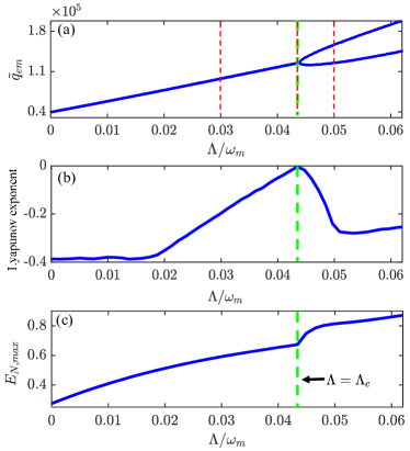
Figure 6: (Color online) (a) Asymptotic extreme values of the mechanical coordinate $\tilde{q}_{em}$ in the classical dynamics, (b) Lyapunov exponent, and (c) $E_{N,max}$ versus parametric gain $\Lambda/\omega_{m}$. Typical bifurcation diagram is found in $\tilde{q}_{em}$. The green dash line indicates the critical point $\Lambda_{c}/\omega_{m}=0.043$ at which the transition from the regular periodic to period-doubling motion occurs. The Lyapunov exponent is taken from the slope of the time-evolutional curve of $\text{ln}(\varepsilon_{I_{c}})$ for the time interval [$280\tau$, $300\tau$] by using linear fitting, with $\vec{\varepsilon}(t=0)=(10^{-10},10^{-10},10^{-10},10^{-10})$. Other parameters are the same as in Fig. 5. The red dashed lines indicate the parametric regime discussed in Figs. 7-9.

As a route to chaos, the period-doubling phenomena were previously discussed in standard optomechanical systems Ma_pra2014 by focusing on the classical nonlinear regime. Here, the main concern is about the quantum entanglement near the classical transitions. For chaotic dynamics, the light-mechanical entanglement can not be measured by the logarithmic negativity any more since the Lyapunov exponent is positive, see further discussion below. Thus, we devote the task to the quantum manifestations of the two common types of classical nonlinear behaviors: regular periodic oscillations and period-doubling motion. However, the entanglement dynamics in chaotic regime may be studied by other methods, such as trajectory-based calculation of the density linear entropy Xu_pra2017 . In Fig. 6(a), we show the asymptotic extreme values $\tilde{q}_{em}$ of the dynamical variable $\tilde{q}$ as a function of the parametric gain $\Lambda$ with Eq. (13). Due to the OPA-modulated driven-dissipative dynamics, the unique extreme value $\tilde{q}_{em}$ separates into two branches as the parametric gain sweeps through the critical OPA pumping $\Lambda_{c}$, and the oscillation amplitude continuously increases for $\Lambda>\Lambda_{c}$.

Furthermore, we study the time-dependence of the Lyapunov exponent Oseledec_TMM1968 , which is defined by the curve slope of the natural logarithms of $\varepsilon_{I_{c}}(t)=\varepsilon_{\alpha_{r}}^{2}+\varepsilon_{\alpha_{i}}^{2}+2\alpha_{r}\varepsilon_{\alpha_{r}}+2\alpha_{i}\varepsilon_{\alpha_{i}}$ versus the evolutional time. The Lyapunov exponent shows how the initial states of cavity field evolve in temporal domain and phase space [see Fig. 6(b)] Ma_pra2014 . One can see that the Lyapunov exponent is negative for $\Lambda<\Lambda_{c}$. While the pumping strength approaches the transition point, the Lyapunov exponent goes to zero. For $\Lambda>\Lambda_{c}$, where the period-doubling motion is found, the Lyapunov exponent falls below zero again. In general, there is no positive Lyapunov exponent for the pumping strength under consideration, which implies that the Gaussian nature of the random noise is well maintained for the quantum Langevin equation and the quantum fluctuation (and therefore the quantum entanglement) can be safely characterized by using the covariance matrix Wang_prl2014 .

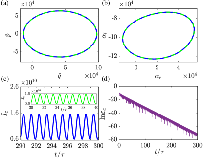
Figure 7: (Color online) Phase space trajectories of (a) the mechanical mode and (b) the cavity mode for time intervals [$30\tau$, $40\tau$] (green dashed lines), [$290\tau$,$300\tau$] (blue lines). (c) Time-dependence of the cavity intensity $I_{c}$ for the time interval [$290\tau$, $300\tau$] in comparison with that for the interval [$30\tau$, $40\tau$] (the inset). (d) Time-dependence of $\text{ln}(\varepsilon_{I_{c}})$ in [$0$,$300\tau$]. Parameters are $\Lambda/\omega_{m}=0.03$, $\vec{\varepsilon}(t=0)=(10^{-10},10^{-10},10^{-10},10^{-10})$. Other parameters are the same as in Fig. 5.

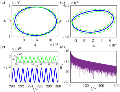
Figure 8: (Color online) Phase space trajectories of (a) the mechanical mode and (b) the cavity mode for time intervals [$30\tau$, $40\tau$] (green dashed lines), [$290\tau$,$300\tau$] (blue lines). (c) Time-dependence of the cavity intensity $I_{c}$ for the time interval [$290\tau$, $300\tau$] in comparison with that for the interval [$30\tau$, $40\tau$] (the inset). (d) Time-dependence of $\text{ln}(\varepsilon_{I_{c}})$ in [$0$,$300\tau$]. Parameters are $\Lambda/\omega_{m}=0.043$, $\vec{\varepsilon}(t=0)=(10^{-10},10^{-10},10^{-10},10^{-10})$. Other parameters are the same as in Fig. 5.

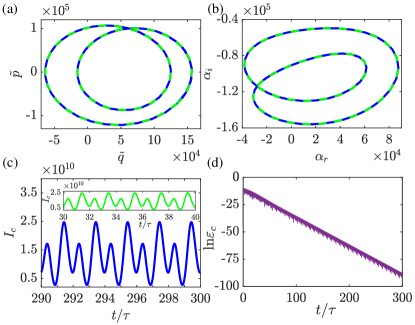
Figure 9: (Color online) Phase space trajectories of (a) the mechanical mode and (b) the cavity mode for time intervals [$30\tau$, $40\tau$] (green dashed lines), [$290\tau$,$300\tau$] (blue lines). (c) Time-dependence of the cavity intensity $I_{c}$ for the time interval [$290\tau$, $300\tau$] in comparison with that for the interval [$30\tau$, $40\tau$] (the inset). (d) Time-dependence of $\text{ln}(\varepsilon_{I_{c}})$ in [$0$,$300\tau$], respectively. Parameters are $\Lambda/\omega_{m}=0.05$, $\vec{\varepsilon}(t=0)=(10^{-10},10^{-10},10^{-10},10^{-10})$. Other parameters are the same as in Fig. 5.

Fig. 6(c) shows the maximum light-mechanical entanglement $E_{N,max}$ as a function of $\Lambda$. One can see that before transition the quantum entanglement smoothly increases with the increasing parametric gain $\Lambda$, but a “cusp” appears at the transition point $\Lambda_{c}$, signified by a sudden increase of entanglement. After the transition, the classical dynamics becomes period-doubling motion, and the quantum entanglement recovers the smoothly increasing characteristic. The general feature resembles to the classical bifurcation followed by the saturation to a stable attractor induced by nonlinear interactions Wang_prl2014 . However, this is described as a characteristic of second-order phase transition in quantum mechanics since the derivatives of the quantum entanglement versus $\Lambda$ are not continuous near the transition point Ying_pra2014 . This implies that a second-order, cusp type of phase transition in light-mechanical entanglement occurs by the aid of OPA in this optomechanical system. As a result, the OPA-modulated driven-dissipative dynamics evokes a classically nonlinear period-doubling behavior accompanied by the appearance of a second order transition in optomechanical entanglement at the critical OPA gain.

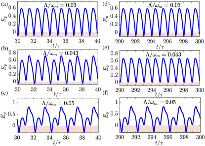
Figure 10: (Color online) Short-time dynamics [(a)-(c)] and long-time dynamics [(d)-(f)] of $E_{P}$ for $\Lambda/\omega_{m}=0.03$ [(a),(d)], $0.043$ [(b),(e)], and $0.05$ [(c),(f)]. Other parameters are the same as in Fig. 6.

To further investigate the dynamical behavior near the transition point in more detail, we show in Figs. 7-9 the steady-state phase-space trajectory of the mechanical and cavity modes, the steady-state cavity intensity $I_{c}$, and the logarithmic deviation $\text{ln}(\varepsilon_{I_{c}})$ for $\Lambda/\omega_{m}=0.03$, $0.043$ and $0.05$ [indicated by red dash lines in Fig. 6 (a)], which correspond to the regular periodic oscillation regime, the transition point and the period-doubling regime, respectively. For $\Lambda/\omega_{m}=0.03$, the classical mean values of the cavity and mechanical modes finally converge to a regular limit cycle for the evolution time less than $30\tau$, and the cavity intensity $I_{c}$ oscillates with the period of $\tau=2\pi/\text{$\Omega$}$, see Fig. 7. In addition, the calculated exponential variation of $\varepsilon_{I_{c}}$ infinitely approaches to zero as time evolves, manifesting that all the nearby points of the initial cavity intensity $I_{c}$ in phase space will finally oscillate in the identical frequency $\Omega$. For $\Lambda/\omega_{m}=0.05$, the phase-space trajectory of the cavity and mechanical modes and time-dependence of cavity intensity then demonstrates the period-doubling motion. Remarkably, the dynamical behavior in this regime can also be observed for a short evolution time $\sim 30\tau$. The fast decrease of $\text{ln}(\varepsilon_{I_{c}})$ over time also signifies that the system can evolve onto its stable orbit rapidly.

While for $\Lambda/\omega_{m}=0.043$, in the vicinity of transition point, the system first experiences a transient period-doubling motion [see the inset of Fig. 8(c)], and then displays a sinusoidal-like oscillation after a long evolution time $\sim 300\tau$, as indicated by the limit-cycle in phase space [see Fig. 8(a)-(b)]. The translational behavior can be further understood by the slow-evolution property of $\text{ln}(\varepsilon_{I_{c}})$ shown in Fig. 8(d) by comparing with that for $\Lambda/\omega_{m}=0.03$ and $\Lambda/\omega_{m}=0.05$.

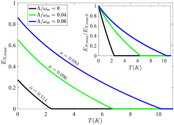
Figure 11: (Color online) $E_{N,max}$ as a function of the thermal temperature $T$ for $\Lambda/\omega_{m}=0$ (the black lower line), $0.04$ (the green middle line), and $0.06$ (the blue upper line). $\mu$ is the entanglement to temperature ratio and the inset shows the renormalized $E_{N,max}$. Other parameter are the same as in Fig. 6.

In correspondence to the classical dynamics, the light-mechanical pseudo-entanglement $E_{p}\equiv-\text{ln}2\eta$ for the parametric gains $\Lambda/\omega_{m}=0.03$, $0.043$, $0.05$ exhibits a similar dynamical behavior, as shown in Fig. 10. For $\Lambda/\omega_{m}=0.03$ and $\Lambda/\omega_{m}=0.05$, the dynamical entanglement quickly become stable in a short time, and thus, the time-dependence of $E_{p}$ for the time intervals [$30\tau$, $40\tau$] and [$290\tau$, $300\tau$] are the same. While for $\Lambda/\omega_{m}=0.043$, we again observe the transient and transitional dynamical behavior in $E_{p}$. These are other quantum manifestations of the classical dynamics. Moreover, it should be noted that the pseudo-entanglement $E_{p}$ less than zero actually denotes non-existence of light-mechanical entanglement, therefore, the system exhibits sudden death and rebirth of light-mechanical entanglement over evolutional time.

Finally, the experimental observation of the above interesting behavior can be realized with the set of parameters Ma_pra2014 ; Ying_pra2014 ; Tho_Nat2008 : $L=25$ mm, $F=1.4\times 10^{4}$ , $\omega_{m}=2\pi\times 1$ MHz, $Q=10^{6}$, $m=150$ ng and the driving laser power $P=21.9$ mW and wavelength $\lambda=1064$ nm. In this case, the cavity decay rate is given by $\kappa/2\pi=c/(4FL)\sim 0.21$ MHz and the effective optomechanical coupling strength for $\Lambda=0$ is around $g_{0}/\omega_{m}=0.48$. Thus, the optomechanical cavity is in the resolved-sideband regime as discussed previously, and the system stays far away from the rotating wave approximation regime, where the off-resonant down conversion process leads to the nonvanishing optomechanical entanglement at $T=0$ Genes_PRA2008 . Moreover, by considering a finite environmental temperature $T$, we find that the light-mechanical entanglement can be greatly enhanced in the presence of OPA, as shown in Fig. 11. In particular, the entanglement to temperature ratio $\mu\equiv E_{N,max}(T=0)/T_{E_{N,max}=0}$ as well as the renormalized entanglement $E_{N,max}(T)/E_{N,max}(T=0)$ show that the system is more robust against thermal noise while the OPA pumping strength increases, and thus, the period-doubling motion (e.g. $\Lambda/\omega_{m}=0.06$) is less sensitive to environmental temperature compared with regular periodic motion (e.g. $\Lambda/\omega_{m}=0.04$).

VI CONCLUSION

In summary, we have studied the classical nonlinear dynamics and the light-mechanical entanglement dynamics in a cavity optomechanical system involving an OPA under two different parameter regimes. In one regime, the classical dynamical behavior (i.e. the regular periodic oscillation and the period-doubling motion) can be manifested in the optomechanical entanglement by special modulation of the OPA pumping with the same parameters. For the other parameter condition that also allows to generate mechanical squeezing, we can examine the normal mode splitting effect in optomechanical entanglement, which finds no classical correspondence. The dynamical behavior is also related to the robustness of the system to the environmental temperature, as evidenced by the death and revival of the optomechanical entanglement. The standard optomechanical system with the assistance of OPA therefore provides a nice architecture for studying and exploring the manifestation of classical nonlinear dynamics in quantum entanglement.

- (1) L. Bakemeier, A. Alvermann, and H. Fehske, Phys. Rev. Lett. 114, 013601 (2015).
- (2) E. Ott, Chaos in Dynamical Systems (Cambridge University Press, Cambridge, England, 2002), 2nd ed.
- (3) G.Wang, L. Huang, Y. C. Lai, and C. Grebogi, Phys. Rev. Lett. 112, 110406 (2014).
- (4) M. V. Berry and M. Robnik, J. Phys. A Math. and Gen. 19, 649 (1986).
- (5) Y. C. Lai, R. BlÃŒmel, E. Ott, and C. Grebogi, ibid. 68, 3491 (1992).
- (6) F. Haake, Quantum Signatures of Chaos, (Springer-Verlag, Berlin, 2010), 3rd ed.
- (7) A. Einstein, B. Podolsky, and N. Rosen, Phys. Rev. 47, 777 (1935).
- (8) S. H. Zhang and Q. L. Jie, Phys. Rev. A 77, 012312 (2008).
- (9) N. Lambert, C. Emary, and T. Brandes, Phys. Rev. Lett. 92, 073602 (2004).
- (10) O. V. Zhirov and D. L. Shepelyansky, Phys. Rev. B 80, 014519 (2009).
- (11) T. E. Lee and H. R. Sadeghpour, Phys. Rev. Lett. 111, 234101 (2013).
- (12) M. Aspelmeyer, T. J. Kippenberg, and F. Marquardt, Rev. Mod. Phys. 86, 1391 (2014).
- (13) F. Marquardt, J. P. Chen, A. A. Clerk, and S. M. Girvin, Phys. Rev. Lett. 99, 093902 (2007).
- (14) I. Wilson-Rae, N. Nooshi, W. Zwerger, and T. J. Kippenberg, Phys. Rev. Lett. 99, 093901 (2007).
- (15) J. D. Teufel, T. Donner, D. Li, J. H. Harlow, M. S. Allman, K. Cicak, A. J. Sirois, J. D. Whittaker, K. W. Lehnert, and R. W. Simmonds, Nature (London) 475, 359 (2011).
- (16) P. Rabl, Phys. Rev. Lett. 107, 063601 (2011).
- (17) X. W. Xu, Y. J. Li, and Y. X. Liu, Phys. Rev. A 87, 025803 (2013).
- (18) Y. Li, Y. Y. Huang, X. Z. Zhang, and L. Tian, Opt. Express 25, 018907 (2017).
- (19) M. P. Blencowe and M. N. Wybourne, Physica (Amsterdam) 280B, 555 (2000).
- (20) H. Tan, Phys. Rev. A 89, 053829 (2014).
- (21) J. Q. Liao and L. Tian, Phys. Rev. Lett. 116, 163602 (2016).
- (22) Jie Li, S. Gröblacher, S. Y Zhu, and G. S. Agarwal, Phys. Rev. A 98, 011801(R) (2018).
- (23) D. Vitali, S. Gigan, A. Ferreira, H. R. Böhm, P. Tombesi, A. Guerreiro, V. Vedral, A. Zeilinger, and M. Aspelmeyer, Phys. Rev. Lett. 98, 030405 (2007).
- (24) Y. D. Wang and A. A. Clerk, Phys. Rev. Lett. 110, 253601 (2013).
- (25) R. X. Chen, L. T. Shen, Z. B. Yang, H. Z. Wu, and S. B. Zheng, Phys. Rev. A 89, 023843 (2014).
- (26) J. Q. Liao, C. K. Law, L. M. Kuang, and F. Nori, Phys. Rev. A 92, 013822 (2015).
- (27) Jie Li, Shi-Yao Zhu, and G. S. Agarwal, Phys. Rev. Lett. 121, 203601 (2018).
- (28) S. Mancini, V. I. Manko, and P. Tombesi, Phys. Rev. A 55, 3042 (1997).
- (29) S. Bose, K. Jacobs, and P. L. Knight, Phys. Rev. A 59, 3204 (1999).
- (30) J. Zhang, K. Peng, and S. L. Braunstein, Phys. Rev. A 68, 013808 (2003).
- (31) M. Pinard, A. Dantan, D. Vitali, O. Arcizet, T. Briant, and A. Heidmann, Europhys. Lett. 72, 747 (2005).
- (32) M. D. LaHaye, O. Buu, B. Camarota, and K. C. Schwab, Science 304, 74 (2004).
- (33) A. Kronwald, F. Marquardt, and A. A. Clerk, Phys. Rev. A 88, 063833 (2013).
- (34) E. E.Wollman, C. U. Lei, A. J.Weinstein, J. Suh, A. Kronwald, F. Marquardt, A. A. Clerk, and K. C. Schwab, Science 349, 952 (2015).
- (35) C. U. Lei, A. J.Weinstein, J. Suh, E. E.Wollman, A. Kronwald, F. Marquardt, A. A. Clerk, and K. C. Schwab, Phys. Rev. Lett. 117, 100801 (2016).
- (36) G. S. Agarwal and S. M. Huang, Phys. Rev. A 93, 043844 (2016).
- (37) C. S. Hu, Z. B. Yang, H. Z. Wu, Y. Li, and S. B. Zheng, Phys. Rev. A 98, 023807 (2018).
- (38) T. Carmon, M. C. Cross, and K. J. Vahala, Phys. Rev. Lett. 98, 167203 (2007).
- (39) J. Larson and M. Horsdal, Phys. Rev. A 84, 021804(R) (2011).
- (40) J. Y. Ma, C. You, L. G. Si, H. Xiong, J. H. Li, X. X. Yang, and Y. Wu, Phys. Rev. A 90, 043839 (2014).
- (41) X. Y. L’́u, H. Jing, J. Y. Ma, and Y. Wu, Phys. Rev. Lett. 114, 253601 (2015).
- (42) F. Bemani, Ali Motazedifard, R. Roknizadeh, M. H. Naderi, and D. Vitali, Phys. Rev. A 96, 023805 (2017).
- (43) A. Mari, A. Farace, N. Didier, V. Giovannetti, and R. Fazio, Phys. Rev. Lett. 111, 103605 (2013).
- (44) M. Ludwig and F. Marquardt, Phys. Rev. Lett. 111, 073603 (2013).
- (45) C. G. Liao, R. X. Chen, H. Xie, M. Y. He, and Xiu-Min Lin, Phys. Rev. A 99, 033818 (2019).
- (46) L. Ying, Y. C. Lai, and C. Grebogi, Phys. Rev. A 90, 053810 (2014).
- (47) C. C. Gerry and P. L. Knight, Introductory Quantum Optics (Cambridge University Press, Cambridge, 2005).
- (48) S. Pina-Otey, F. Jimenez, P. Degenfeld-Schonburg, and C. Navarrete-Benlloch, Phys. Rev. A 93, 033835 (2016).
- (49) S. M. Huang and G. S. Agarwal, Phys. Rev. A 80, 033807 (2009).
- (50) S. M. Huang and G. S. Agarwal, Phys. Rev. A 79, 013821 (2009).
- (51) X. Y. L’́u, Y. Wu, J. R. Johansson, H. Jing, J. Zhang, and F. Nori, Phys. Rev. Lett. 114, 093602 (2015).
- (52) C. W. Gardiner and P. Zoller, Quantum Noise, (Springer, New York, 2004), 3rd ed.
- (53) V. Giovannetti and D. Vitali, Phys. Rev. A 63, 023812 (2001).
- (54) A. Farace and V. Giovannetti, Phys. Rev. A 86, 013820 (2012).
- (55) A. Mari and J. Eisert, Phys. Rev. Lett. 103, 213603 (2009).
- (56) A. Mari and J. Eisert, New J. Phys. 14, 075014 (2012).
- (57) S. M. Huang and G. S. Agarwal, Phys. Rev. A 81, 033830 (2010).
- (58) J. D. Thompson, B. M. Zwickl, A. M. Jayich, Florian Marquardt, S. M. Girvin, and J. G. E. Harris, Nature (London) 452, 72 (2008).
- (59) S. D. Gupta and G. S. Agarwal, Opt. Commun. 115, 597 (1995).
- (60) F. Xu, C. C. Martens, and Y. Zheng, Phys. Rev. A 96, 022138 (2017).
- (61) V. I. Oseledet, Trans. Mosc. Math. Soc. 19, 197 (1968).
- (62) C. Genes, A. Mari, P. Tombesi, and D. Vitali, Phys. Rev. A 78, 032316 (2008).