A stochastic alternating minimizing method for sparse phase retrieval

Abstract

Spares phase retrieval plays an important role in many fields of applied science and thus attracts lots of attention. In this paper, we propose a stochastic alternating minimizing method for sparse phase retrieval (StormSpar) algorithm which emprically is able to recover $n$-dimensional $s$-sparse signals from only $O(s\,\mathrm{log}\,n)$ number of measurements without a desired initial value required by many existing methods. In StormSpar, the hard-thresholding pursuit (HTP) algorithm is employed to solve the sparse constraint least square sub-problems. The main competitive feature of StormSpar is that it converges globally requiring optimal order of number of samples with random initialization. Extensive numerical experiments are given to validate the proposed algorithm.

I Introduction

Phase retrieval is to recover the phase information from its magnitude measurements, i.e.,

$$y_{i}=|\langle a_{i},x\rangle|+\epsilon_{i},\quad i=1,2,\cdots,m,$$ (1)

where $x\in\mathbb{F}^{n}$ is the unknown vector, $a_{i}\in\mathbb{F}^{n}$ are given sampling vectors which are random Gaussian vector in this paper, $y_{i}$ is the observed measurements, $\epsilon_{i}$ is the noise, and $m$ is the number of measurements (or the sample size). The $\mathbb{F}^{n}$ can be $\mathbb{R}^{n}$ or $\mathbb{C}^{n}$, and we consider the real case $\mathbb{F}^{n}=\mathbb{R}^{n}$ in this work. The phase retrieval problem arises in many fields like X-ray crystallography [1], optics [2], microscopy [3] and others, see e.g., [4]. Due to the lack of phase information, the phase retrieval problem is a nonlinear and ill-posed problem.

When the measurements are overcomplete i.e., $m>n$, there are many algorithms in the literatures. Earlier approaches were mostly based on alternating projections, e.g. the work of Gerchberg and Saxton [5] and Fienup [4]. Recently, convex relaxation methods such as phase-lift [6] and phase-cut [7] have been proposed. These methods transfer the phase retrieval problem into a semi-definite programing, which can be computationally expensive. Another convex approach named phase-max which does not lift the dimension of the signal was proposed in [8]. In the mean while, there are other works based on solving nonconvex optimization via first and second order methods including alternating minimization [9] (or Fienup methods), Wirtinger flow [6] Kaczmarz [10], Riemannian optimization [11]; Gauss-Newton [12, 13] etc. With a good initialization abstained via spectral methods, the above mentioned methods work with theoretical guarantees. Progresses have been made by replacing the desired initialization with random initialized ones in alternating minimization [14, 15], gradient descent [16] and Kaczmarz method [17, 18] while keeping convergence guarantee with high probability. Also, recent analysis in [19, 20] has shown that some nonconvex objective functions for phase retrieval have a nice landscape — there is no spurious local minima — with high probability. As a consequence, for these objective functions, any algorithms finding a local minima are guaranteed to give a successful phase retrieval.

For the large scale problem, the requirement $m>n$ becomes unpractical due to the huge measurement and computation cost. In many applications, the true signal $x$ is known to be sparse. Then the sparse phase retrieval problem can be solved with a small number of sampling, thus possible to be applied to large scale problems. It has been proved in [21] that $m=O(s\mathrm{log}\,n/s)$ measurement is sufficient to ensure successful recovery in theory with high probability when the model is Gaussian (i.e. the sampling vector $a_{i}$ are i.i.d Gaussian and the target is real). But the exiting computational trackable algorithms require $O(s^{2}\mathrm{log}\,n)$ number of measurements to reconstruct the sparse signal, for example, $\ell_{1}$ regularized PhaseLift method [22], sparse AltMin [9], GESPAR [23], Thresholding/projected Wirtinger flow [24, 25], SPARTA [26] and so on. Two stage methods based on phase-lift and compressing has been introduced in [27, 28], which is able to do successful reconstruction with $O(s\mathrm{log}\,n)$ measurements for some special designed sampling matrix which exclude the Gaussian model (1). When a good initialization is available, the sample complexity can be improved to $O(s\mathrm{log}\,n)$ [29, 25]. However, it requires $O(s^{2}\mathrm{log}\,n)$ samples to get a desired sparse initialization in the existing literatures. This gap naturally raises the following challenging question

Can one recover the $s$-sparse target from the phaseless generic Gaussian model (1) with $O(s\mathrm{log}\,n)$ measurements via just using random initializations ?

In this paper, we propose a novel algorithm to solve the sparse phase retrieval problems in the very limited measurements (numerical examples show that $m=O(s\mathrm{log}\,n)$ can be enough). The algorithm is a stochastic version of alternating minimizing method. The idea of alternating minimization method is: during each iteration, we first given an estimation of the phase information, then substitute the approximated phase into (1) with the sparse constraint and solve a standard compressed sensing problem to get an updated sparse signal. But since the alternating minimizing method is a local method, it is very sensitive to the initialization. Without enough measurements, it is very difficult to compute a good initial guess. To overcome this difficult, we change the sample matrix during each iteration via bootstrap technique, see Algorithm 1 for details. The numerical experiments shows that the proposed algorithm needs only $O(s\,\mathrm{log}\,n)$ measurements to recover the true signal with high probability in Gaussian model, and it works for a random initial guess. The experiments also show that the proposed algorithm is able to recover signal in a wide range of sparsity.

The rest of papers are as follows. In section II we will introduce the setting of problem and the details of the algorithm. Numerical experiments are given in section III.

II Algorithm

First we introduce some notations. For any $a,b\in\mathbb{R}^{n}$, we denote that $a\odot b=(a_{1}b_{1},a_{2}b_{2},\cdots,a_{n}b_{n})$, $\lVert x\lVert_{0}$ is the number of nonzero entries of $x$, and $\lVert x\lVert_{2}$ is the standard $\l_{2}$-norm, i.e. $\lVert x\lVert_{2}=\sqrt{\sum_{i=i}^{n}x_{i}^{2}}$. The floor function $\lfloor c\rfloor$ is the greatest integer which is less than or equal to $c$.

Recall from (1), We denote the sampling matrix and the measurement vector by $A=[a_{1}^{t};...;a_{m}^{t}]\in\mathbb{R}^{m\times n}$ and $y=[y_{1};...;y_{m}]\in\mathbb{R}^{m}$, respectively. Let $x\in\mathbb{R}^{n}$ be the unknown sparse signal to be recovered. In the noise free case, the problem can be written as to find $x$ such that

$$y=\lvert Ax\lvert,\quad\mathrm{s.t}\ \lVert x\lVert_{0}\leq s.$$

In the noise case, this can be written by the nonconvex minimization problem:

$$\min_{x}\quad\frac{1}{2}\lVert y-|Ax|\lVert_{2}^{2}\quad\mathrm{s.t.}\ \lVert x\lVert_{0}\leq s\;,$$ (2)

Now we propose the stochastic alternating minimizing method for sparse phase retrieval (StormSpar) as follows. It starts with a random initial guess $x^{0}$. In the $\ell$-th step of iteration ($\ell=1,2,\cdots$), we first randomly choose some rows of the sampling matrix $A$ to form a new matrix $A^{\ell}$ (which is a submatrix of $A$), and denoted by the corresponding rows of $y$ to $A^{\ell}$ is $y^{\ell}$. Then we compute the phase information of $A^{\ell}x^{\ell-1}$, say $p^{\ell}=\mathrm{sign}(A^{\ell}x^{\ell-1})$, and to solve the standard compressed sensing subproblem

$$\min_{x}\frac{1}{2}\|A^{\ell}x-\tilde{y}^{\ell}\|^{2}\quad\mathrm{s.t.}\ \lVert x\lVert_{0}\leq s\;,$$ (3)

where $\tilde{y}^{\ell}=p^{\ell}\odot y^{\ell}$. Problem (3) can be solved by a lot of compressed sensing solver, and we will use the efficient Hard Thresholding Pursuit (HTP) [30] in our algorithm. For completion, HTP is given in Algorithm 2. We summarize the StormSpar algorithm in the Algorithm 1.

III Numerical Results and Discussions

III-A Implementation details

The true signal $x$ is chosen as $s$-sparse with random support and the design matrix $A\in\mathbb{R}^{m\times n}$ is chosen to be random Gaussian matrix. The additive gaussian noise following the form $\epsilon=\sigma*\textrm{randn}(n,1)$, thus the noise level is determined by $\sigma$. The parameter $\gamma$ is set to be $\mathrm{min}(\frac{s}{m}*\mathrm{log}\,\frac{n}{0.001},0.6)$, and $\delta=0.01$.

The estimation error $r$ between the estimator $\hat{x}$ and the true signal $x$ is defined as

$$r=\min\{\|\hat{x}+x\|_{2},\|\hat{x}-x\|_{2}\}/\|x\|_{2}.$$

We say it is a successful recovery when the relative estimation error $r$ satisfy that $r\leq 1e-2$ or the support is exactly recovered. The tests repeat independently for $100$ times to compute a successful rate. “Aver Iter” in the table I and II means the average number of iterations for 100 times of tests. All the computations were performed on an eight-core laptop with core i7 6700HQ@3.50 GHz and 8 GB RAM using MATLAB 2018a.

Algorithm 1 StormSpar

1:  Input: Normalized $A\in\mathbb{R}^{m\times n}$, $y$, sparsity level $s$, $\gamma\in(0,1)$, small constant $\delta$, a random initial value $x^{0}$.

2:  for $\ell=1,2,...$ do

3:     Randomly selected $\lfloor\gamma m\rfloor$ rows of $A$ and $y$, denote the index as $i^{\ell}$, to form $A^{\ell}=A(i^{\ell},:)$ $y^{\ell}=y(i^{\ell})$.

4:     Compute $p^{\ell}=\mathrm{sign}(A^{\ell}x^{\ell-1}),\tilde{y}^{\ell}=p^{\ell}\odot y^{\ell}$.

5:     Get $x^{\ell}$ by solving $\min_{x,\|x\|_{0}\leq s}\frac{1}{2}\|A^{\ell}x-\tilde{y}^{\ell}\|^{2}$ via Algorithm 2 (HTP).

6:     Check stop criteria ${\lVert x^{\ell}-x^{\ell-1}\rVert}\leq\delta$.

7:  end for

8:  Get the first $s$ position of $x^{\ell}$ and refit on it as output.

Algorithm 2 HTP solving (3)

1:  Input: Initialization: $k=0,x^{0}=0;$

2:  for $k=1,2,...$ do

3:     $S^{k}\leftarrow$ {indices of s largest entries of $x^{k-1}+\mu(A^{\ell})^{t}(\tilde{y}^{\ell}-A^{\ell}x^{k-1})$};

4:     Solve $x^{k}\leftarrow\mathrm{argmin}_{\mathrm{supp}(x)\subset S^{k}}\lVert A^{\ell}x-\tilde{y}^{\ell}\lVert_{2}.$

5:  end for

III-B Examples

Example 1 First we examine the effect of sample size $m$ to the probability of successful recovery in Algorithm 1. The dimension of the signal $x$ is $n=1000$.
a.) When we set sparsity to be $s=10,25,50$, Fig. 1 shows how the successful rate changes in terms of the sample size $m$. In this experiment, we fix a number $K=\lfloor(s(\mathrm{log}\,n+\mathrm{log}\,\frac{1}{0.01}))\rfloor$, which is $115,287,575$ with respect to the sparsity $10,25,50$. Then we compute the probability of success when $m/K$ changes: for each $s$ and each $m/K=1,1.25,\cdots,3$, we run our algorithm for $100$ times. We find it that when the sample size is in order $O(s\,\mathrm{log}\,n)$ in this setting, we can recover the signal with high possibility.

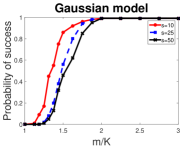
Figure 1: The probability of success in recovery v.s. sample size $m/K$ for Gaussian model, $K=\lfloor(s(\mathrm{log}\ n+\mathrm{log}\frac{1}{0.01}))\rfloor$ which is $115,287,575$ with respect to sparsity $s=10,25,50$, signal dimension $n=1000$, noise level $\sigma=0.01$.

b.) We compare StormSpar to some existing algorithm, i.e. CoPRAM[31], Thresholded Wirtinger Flow(ThWF)[24] and SPArse truncated Amplitude flow (SPARTA)[26]. The sparsity is set to be $30$ and the model is noise free. Fig. 2 shows the successful rate comparison in terms of sample size, the results are obtained by averaging the results of $100$ trials. We find it that StormSpar requires more iterations and more cpu time than these algorithms which requires initialization. But StormSpar achieves better accuracy with less sample complexity.

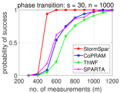
Figure 2: The probability of success in recovery for different algorithms in terms of changing sample size, dimension $n=1000$, sparsity $s=30$ and the model is noise free.

Example 2 Fig. 3 shows that StormSpar is robust to noise. We set $n=1000,s=20$, and $m=\lfloor(2.5s(\mathrm{log}\ n+\mathrm{log}\frac{1}{0.01}))\rfloor(=575)$. The noise we added is i.i.d. Gaussian, and the noise level is shown by signal-to-noise ratios (SNR), we plot the corresponding relative error of reconstruction in the Fig. 3. The results are obtained by average of $100$ times trial run.

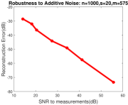
Figure 3: The reconstruction error v.s. SNR to measurements for Gaussian model, $m=\lfloor(2.5s(\mathrm{log}\ n+\mathrm{log}\frac{1}{0.01}))\rfloor=575$ with sparsity $s=20$, signal dimension $n=1000$ and several noise level, i.e. SNR to measurements.

Example 3 We compare StormSpar with a two-stage method Phaselift+BP proposed in [27], which has been shown to be more efficient than the standard SDP of [32]. The dimension of data is set to be $n=1000$. The comparison are two-folder. Firstly, we compare the minimum number of measurements required to be sample size which gives successful recovery rate higher than $95\%$ for different sparsity level, the result can be found in Figure 4. Secondly the average computational time is given in Figure 5, where $m=\lfloor(2.5s(\mathrm{log}\,n+\mathrm{log}\,\frac{1}{0.01}))\rfloor$.

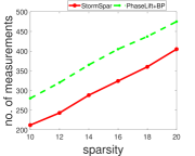
Figure 4: Comparison of Minimum number of measurements required for Gaussian model, signal dimension $n=1000$ and free of noise.

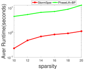
Figure 5: Comparison of efficiency for Gaussian model, signal dimension $n=1000$ and free of noise.

Example 4 Let $m=O(s\mathrm{log}\,n)$, we test for different sparse levels and differen dimensions. In Table I, we fix dimension $n=2000$, and the sample size is chosen to be $m=\lfloor(2.5s(\mathrm{log}\,n+\mathrm{log}\,\frac{1}{0.01}))\rfloor$. The sparsity level chages from $5$ to $100$, we find the algorithm can successfully recover the sparse signal in most case, and the iteration number is very stable.

In Table II, the sparsity level is fixed by $s=10$, the sample size is $m=\lfloor(2.5s(\mathrm{log}\,n+\mathrm{log}\,\frac{1}{0.01}))\rfloor$ for dimension $n$ from $100$ to $10000$. We find the algorithm can successfully recover the sparse signal in most cases, and the number of iteration dependent on the dimension $n$ in a sublinear manner.

Table I: Numerical results for sparsity test, with random sampling $A$ of size $n\times m$, $n=2000$, $m=\lfloor(2.5s(\mathrm{log}\,n+\mathrm{log}\,\frac{1}{0.01}))\rfloor$, $s$ is the sparsity, with $\sigma=\mbox{0.01}$, and Aver Iter$=\lfloor$ average number of iterations for 100 times of test$\rfloor$ .

Dimension $n$	Sparsity $s$	Sample $m$	Successful Rate	Aver Iter
$2000$	5	152	98%	109
$2000$	10	305	99%	229
$2000$	15	457	99%	359
$2000$	20	610	98%	395
$2000$	25	762	100%	407
$2000$	30	915	99%	403
$2000$	35	1068	100%	482
$2000$	40	1220	100%	331
$2000$	45	1373	100%	305
$2000$	50	1525	100%	324
$2000$	75	2288	100%	289
$2000$	100	3051	100%	285

Table II: Numerical results for different dimensions, with random sampling $A$ of size $n\times m$, $m=\lfloor(2.5s(\mathrm{log}\,n+\mathrm{log}\,\frac{1}{0.01}))\rfloor$, $s$ is the sparsity, with $\sigma=\mbox{0.01}$, and Aver Iter$=\lfloor$ average number of iterations for 100 times of test$\rfloor$ .

Dimension $n$	Sparsity $s$	Sample $m$	Successful Rate	Aver Iter
$100$	10	230	98%	38
$200$	10	249	99%	46
$300$	10	257	100%	56
$400$	10	264	100%	72
$500$	10	270	100%	93
$750$	10	280	100%	123
$1000$	10	287	100%	157
$1500$	10	297	99%	192
$2000$	10	305	99%	229
$3000$	10	315	99%	298
$4000$	10	322	98%	508
$5000$	10	328	97%	748
$7500$	10	338	95%	1142
$10000$	10	345	96%	1271

IV Conclusion

In this paper, we have proposed a novel algorithm (StormSpar) for the sparse phase retrieval. StormSpar start with a random initialization and employ a alternating minimizing method for a changing objective function. The subproblem $\min_{x,\|x\|_{0}\leq s}\frac{1}{2}\|A^{\ell}x-\tilde{y}^{\ell}\|^{2}$ is a standard compressed sensing problem, which can be solved by HTP method. Numerical exampls show that the proposed algorithm requires only $O(s\,\mathrm{log}\,n)$ samples to recover the $s$-sparse signal with a random initial guess.

References

- [1] R. W. Harrison, “Phase problem in crystallography,” JOSA a, vol. 10, no. 5, pp. 1046–1055, 1993.
- [2] A. Walther, “The question of phase retrieval in optics,” Journal of Modern Optics, vol. 10, no. 1, pp. 41–49, 1963.
- [3] J. Miao, T. Ishikawa, Q. Shen, and T. Earnest, “Extending x-ray crystallography to allow the imaging of noncrystalline materials, cells, and single protein complexes,” Annu. Rev. Phys. Chem., vol. 59, pp. 387–410, 2008.
- [4] J. R. Fienup, “Phase retrieval algorithms: a comparison,” Applied optics, vol. 21, no. 15, pp. 2758–2769, 1982.
- [5] R. W. Gerchberg, “A practical algorithm for the determination of the phase from image and diffraction plane pictures,” Optik, vol. 35, pp. 237–246, 1972.
- [6] E. J. Candes, Y. C. Eldar, T. Strohmer, and V. Voroninski, “Phase retrieval via matrix completion,” SIAM review, vol. 57, no. 2, pp. 225–251, 2015.
- [7] I. Waldspurger, A. d Aspremont, and S. Mallat, “Phase recovery, maxcut and complex semidefinite programming,” Mathematical Programming, vol. 149, no. 1-2, pp. 47–81, 2015.
- [8] T. Goldstein and C. Studer, “Phasemax: Convex phase retrieval via basis pursuit,” IEEE Transactions on Information Theory, vol. 64, no. 4, pp. 2675–2689, 2018.
- [9] P. Netrapalli, P. Jain, and S. Sanghavi, “Phase retrieval using alternating minimization,” in Advances in Neural Information Processing Systems, 2013, pp. 2796–2804.
- [10] K. Wei, “Solving systems of phaseless equations via kaczmarz methods: A proof of concept study,” Inverse Problems, vol. 31, no. 12, p. 125008, 2015.
- [11] J.-F. Cai and K. Wei, “Solving systems of phaseless equations via Riemannian optimization with optimal sampling complexity,” arXiv preprint arXiv:1809.02773, 2018.
- [12] B. Gao and Z. Xu, “Gauss-newton method for phase retrieval,” IEEE Transactions on Signal Processing, vol. 65, no. 22, pp. 5885–5896, 2017.
- [13] C. Ma, X. Liu, and Z. Wen, “Globally convergent levenberg-marquardt method for phase retrieval,” IEEE Transactions on Information Theory, 2018.
- [14] I. Waldspurger, “Phase retrieval with random gaussian sensing vectors by alternating projections,” IEEE Transactions on Information Theory, vol. 64, no. 5, pp. 3301–3312, 2018.
- [15] T. Zhang, “Phase retrieval using alternating minimization in a batch setting,” Applied and Computational Harmonic Analysis, 2019.
- [16] Y. Chen, Y. Chi, J. Fan, and C. Ma, “Gradient descent with random initialization: Fast global convergence for nonconvex phase retrieval,” Mathematical Programming, 2018.
- [17] Y. S. Tan and R. Vershynin, “Phase retrieval via randomized kaczmarz: Theoretical guarantees,” Information and Inference: A Journal of the IMA, vol. 8, no. 1, pp. 97–123, 2018.
- [18] H. Jeong and C. S. G nt rk, “Convergence of the randomized kaczmarz method for phase retrieval,” arXiv preprint arXiv:1706.10291., 2017.
- [19] J. Sun, Q. Qu, and J. Wright, “A geometrical analysis of phase retrieval,” Foundations of Computational Mathematics, vol. 18, no. 5, pp. 1131–1198, 2018.
- [20] Z. Li, J.-F. Cai, and K. Wei, “Towards the optimal construction of a loss function without spurious local minima for solving quadratic equations,” arXiv preprint arXiv:1809.10520, 2018.
- [21] Y. C. Eldar and S. Mendelson, “Phase retrieval: Stability and recovery guarantees,” Applied and Computational Harmonic Analysis, vol. 36, no. 3, pp. 473–494, 2014.
- [22] X. Li and V. Voroninski, “Sparse signal recovery from quadratic measurements via convex programming,” SIAM Journal on Mathematical Analysis, vol. 45, no. 5, pp. 3019–3033, 2013.
- [23] Y. Shechtman, A. Beck, and Y. C. Eldar, “Gespar: Efficient phase retrieval of sparse signals,” IEEE transactions on signal processing, vol. 62, no. 4, pp. 928–938, 2014.
- [24] T. T. Cai, X. Li, and Z. Ma, “Optimal rates of convergence for noisy sparse phase retrieval via thresholded wirtinger flow,” The Annals of Statistics, vol. 44, no. 5, pp. 2221–2251, 2016.
- [25] M. Soltanolkotabi, “Structured signal recovery from quadratic measurements: Breaking sample complexity barriers via nonconvex optimization,” IEEE Transactions on Information Theory, 2019.
- [26] G. Wang, L. Zhang, G. B. Giannakis, M. Akçakaya, and J. Chen, “Sparse phase retrieval via truncated amplitude flow,” IEEE Transactions on Signal Processing, vol. 66, no. 2, pp. 479–491, 2018.
- [27] M. Iwen, A. Viswanathan, and Y. Wang, “Robust sparse phase retrieval made easy,” Applied and Computational Harmonic Analysis, vol. 42, no. 1, pp. 135–142, 2017.
- [28] S. Bahmani and J. Romberg, “Efficient compressive phase retrieval with constrained sensing vectors,” Advances in Neural Information Processing Systems, pp. 523–531, 2015.
- [29] P. Hand and V. Voroninski, “Compressed sensing from phaseless gaussian measurements via linear programming in the natural parameter space,” arXiv preprint arXiv:1611.05985, 2016.
- [30] S. Foucart, “Hard thresholding pursuit: an algorithm for compressive sensing,” SIAM Journal on Numerical Analysis, vol. 49, no. 6, pp. 2543–2563, 2011.
- [31] G. Jagatap and C. Hegde, “Sample-efficient algorithms for recovering structured signals from magnitude-only measurements,” IEEE Transactions on Information Theory, 2019.
- [32] H. Ohlsson, A. Yang, R. Dong, and S. Sastry, “Cprl–an extension of compressive sensing to the phase retrieval problem,” in Advances in Neural Information Processing Systems, 2012, pp. 1367–1375.